On the algorithm to perform Monte Carlo simulations in cells with constant volume and variable shape

Abstract

In simulations of crystals, unlike liquids or gases, it may happen that the properties of the studied system depend not only on the volume of the simulation cell but also on its shape. For such cases it is desirable to change the shape of the box on the fly in the course of the simulation as it may not be known ahead of time which geometry fits the studied system best. In this work we derive an algorithm for this task based on the condition that the distribution of specific geometrical parameter observed in simulations at a constant volume matches that observed in the constant-pressure ensemble. The proposed algorithm is tested for the system of hard-core ellipses which makes lattices of different types depending on the asphericity parameter of the particle. It is shown that the performance of the algorithm critically depends on the range of the sampled geometrical parameter. If the range is narrow, the impact of the sampling method is minimal. If the range is large, inadequate sampling can lead to significant distortions of the relevant distribution functions and, as a consequence, errors in the estimates of free energy.

Key words: hard-ellipse fluid, Monte Carlo simulation, constant volume, varying shape, umbrella sampling

Abstract

 ñèìóëÿöiÿõ êðèñòàëiâ ïåâíi âëàñòèâîñòi äîñëiäæóâàíî¿ ñèñòåìè ìîæóòü çàëåæàòè íå òiëüêè âiä îá’єìó êîìiðêè ìîäåëþâàííÿ àëå é âiä ¿¿ ôîðìè.  òàêèõ âèïàäêàõ áàæàíî çìiíþâàòè ôîðìó êîìiðêè â ïðîöåñi ñèìóëÿöié, îñêiëüêè íàïåðåä âîíà ìîæå áóòè íåâiäîìîþ. Ó öié ðîáîòi îïèñàíî àëãîðèòì ÿêèé äîçâîëÿє öå ðîáèòè ç òî¿ óìîâè, ùîá âiäòâîðèòè êëþчîâi ïàðàìåòðè ôîðìè êîìiðêè, ÿêi ñïîñòåðiãàþòüñÿ â àíñàìáëi ïðè ïîñòiéíîìó òèñêó. Àëãîðèòì ïðîòåñòîâàíî â ñèìóëÿöiÿõ ñèñòåìè òâåðäèõ åëiïñiâ, ÿêà ìîæå óòâîðþâàòè ãðàòêè ðiçíîãî òèïó. Ïîêàçàíî, ùî âèêîðèñòàííÿ çàïðîïîíîâàíîãî àëãîðèòìó ïðèçâîäèòü äî äîáðîãî óçãîäæåííÿ âiäíîñíî¿ âiëüíî¿ åíåðãi¿ ðiçíèõ òèïiâ ãðàòîê ç ðåçóëüòàòàìè îòðèìàíèìè íåçàëåæíèìè ìåòîäàìè.

Ключовi слова: òâåðäèé åëiïñ, Ìîíòå Êàðëî, àíñàìáëü ïðè ïîñòiéíîìó îá’єìi

1 Introduction

Today computer simulations play a key role in fundamental research across multiple disciplines, including physics, chemistry and materials science [1]. A large share of computational studies employ simulation boxes with fixed volume. This choice is mainly motivated by convenience as constant-volume/constant-temperature ensemble is easier to program than the equivalent ensemble with constant pressure. But this is also due to the involvement of the constant-volume ensemble in other, specialized simulation techniques such as free energy calculations [2], Gibbs ensemble [3] or replica-exchange method [4, 5, 6]. Regardless of the particular context, it is always understood that the effect of volume vanishes in the thermodynamic limit where the results are thought to be independent of the employed ensemble. This claim is certainly true for liquids or gases, whose properties are independent of the geometry of the box.

In the case of crystals, however, the situation could be quite different [7, 8]. In crystalline materials there could be properties that depend explicitly on the volume as well as on the shape of the box. Take for instance the example of a rectangular lattice with lattice constants $a$ and $b$, as shown in figure 1. The dimensions of the box that accommodates $n$ columns and $m$ rows are $L_{x}=an$ along $x$ axis and $L_{y}=bm$ along $y$ axis as shown in figure 1 (a). The corresponding aspect ratio is $\tau=L_{x}/L_{y}=an/bm$. Now, let us assume that the lattice constants are not known ahead of time but are meant to be determined in the course of the simulations. If we initially choose a box with the wrong aspect ratio, $\tau^{\prime}>\tau$ for instance, see figure 1 (b) for appropriate illustration, the lattice constant determined in simulations will also be incorrect. Since the geometry of the cell drives the structure of the lattice, wrong geometry translates into wrong structure. Importantly, lattice distortions will not go away easily even when the size of the simulation box is increased.

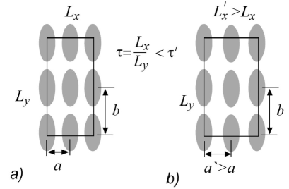
Figure 1: Aspect ratio of simulation boxes is governed by the geometry of the modelled lattice. Incorrect initial guess will result in lattice distortions in constant volume simulations, for instance leading to $a^{\prime}>a$. To circumvent this problem, the box should be capable of changing its shape.

One way to deal with this issue is to estimate the free energy of the studied system $F$ as a function of some geometrical parameter of the cell, for instance $\tau$, and then choose the geometry with the lowest $F$. This can be done by a variety of tools, including the Einstein crystal method for the free energy computation [9, 2]. Although formally correct, this approach is cumbersome and carries a large computational cost. An alternative is to allow the shape of the box to change in the course of the simulation. The proper geometry then corresponds to the free energy minimum, so it will be seen as the most frequently visited structure. An additional benefit will be for systems that can populate multiple geometries at the same time as their relative free energy in this case can be determined from a single Monte Carlo (MC) trajectory.

The question then is how does one allow the shape of the box to change? How is that accomplished in practice? Would, for instance, generating randomly, from time to time, a new aspect ratio $\tau$ in the course of the simulation constitute a good method? If not, what is the good method? These questions had been addressed before as multiple studies report using simulation cells with constant volume but variable shape (MCVS) [10, 11, 7, 8]. Unfortunately, the details of the performed simulations are scarce and to establish the specifics of the used algorithms appears difficult. Yet, we find evidence that the method one employs to sample the trial geometries may have measurable consequences for physical properties extracted from simulations. Thus, which geometry parameters are best to choose in MCVS simulations, and how to choose them remains unclear. These are the questions that we answer in the present article. We show that in order for the constant-volume ensemble with variable shape to be consistent with the constant-pressure ensemble, the aspect ratio should be sampled from the $1/\tau$ distribution. Any other sampling law will lead to erroneous results. We illustrate this point for the system of impenetrable ellipses in two-dimensional space, for which we evaluate the performance of the method that relies on uniformly sampled $\tau$, or on the so-called $\tau$-sampling and show that it produces wrong free energy for the relevant states of the system.

2 Theory

2.1 Sampling law for $\tau$

Let us assume that, in addition to volume, the partition function in the canonical, or NVT for short, ensemble $Q(N,T,V;\tau)=\int_{V;\tau}\rm{exp}[{-\beta U(\Gamma)}]\mathrm{d}\Gamma$ explicitly depends on some geometrical parameter $\tau$, for instance the aspect ratio of the box sides. Here, $\beta$ is the inverse temperature, $V$ is the volume, $U(\Gamma)$ is the potential energy and $\Gamma$ is the abbreviation for the point in the configuration space. The integration is carried out over volume $V$ with the set parameter $\tau$. The full partition function then should be constructed as a weighted sum (or integral) over all possible realizations of the additional degree of freedom [12]. In the most general case, one finds:

$$Q(N,T,V)=\int{Q(N,T,V;\tau)f(\tau)\mathrm{d}\tau=\int{P(\tau)\mathrm{d}\tau}},$$ (2.1)

where $f(\tau)$ is the weighting function of the extended ensemble defined by both volume and the shape of the box and $P(\tau)$ is the probability distribution function of $\tau$, characteristic of the NVT ensemble with variable shape. In principle, one is free to choose $f(\tau)$ arbitrarily, provided that it satisfies certain conditions typically imposed on distribution functions, such as positive definiteness or integrability. Here, we will select $f(\tau)$ on the condition that the extended ensemble with fixed volume satisfies distribution of $\tau$ specific for the constant pressure, or NPT, ensemble. In this way, modelling in the two ensembles, constant-volume and constant-pressure, will be consistent, hence minimizing finite size effects.

The distribution function in the constant-pressure ensemble reads:

$$P(\Gamma,N,T,{\mathcal{P}})\sim\mathrm{e}^{-\beta{\mathcal{P}}V}\ \mathrm{e}^{-\beta U(\Gamma)},$$ (2.2)

where $\mathcal{P}$ is the pressure. Let us focus now on 2D space and obtain formulas for this simpler case first. The relevant volume is $V=L_{x}L_{y}\sin\alpha$, where $L_{x}$ and $L_{y}$ are the lengths of the simulation box and $\sin\alpha$ is the sine of the angle between them. In NPT simulations, volume is sampled randomly from a uniform distribution. This can be achieved either by uniformly sampling one of the variables involved in volume, $L_{x}$, $L_{y}$ or $\sin\alpha$, or by non-uniformly sampling some combination of these variables which leads to a uniformly distributed volume [2]. Let us assume that the first scenario takes place, as it is more general and can be applied to both liquids and crystals, and each concerned variable is sampled uniformly, one at a time and in random order. The joint distribution function measured in such simulations for variables $L_{x}$, $L_{y}$ and $\sin\alpha$ will be given by the following expression:

$$P\left(L_{x},L_{y},\sin\alpha\right)\sim\mathrm{e}^{-\beta{\mathcal{P}}L_{x}L_{y}\sin\alpha}\ Q(N,T,V;\tau),$$ (2.3)

which can also be obtained by integrating distribution function (2.2) over all configurations $\Gamma$. The dependence on $\tau$ in the partition function arises because the integration over $\Gamma$ is carried out for the box with specific dimensions $L_{x}$ and $L_{y}$, which in addition to the volume $V=L_{x}L_{y}$ also define other geometrical parameters including $\tau=L_{x}/L_{y}$.

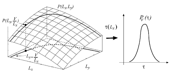
Figure 2: Cartoon illustrating hypothetical joint distribution function of variables $L_{x}$ and $L_{y}$ for the constant-pressure ensemble. Constant-volume configurations correspond to the sub-ensemble bound to the line $L_{y}=V/L_{x}$, where $L_{x}$ is treated as the independent variable. Sampling along this line uniquely defines the distribution function $P_{V}(\tau)$ for geometrical parameter $\tau$.

As an illustration, consider a schematic distribution ${P(L}_{x},L_{y})$ shown in figure 2, specific for rectangular boxes with $\sin\alpha=1$. Among all possible configurations, those that correspond to volume $V$ satisfy the constraint $V=L_{x}L_{y}$, creating a one-dimensional sub-ensemble characterized by a single degree of freedom. If $L_{x}$ is chosen as the independent degree of freedom, configurations with given $V$ and $L_{x}$ will appear in simulations with probability ${P(L}_{x},{V}/{L_{x}})$. Any other geometric parameter of the system will also be characterized by a unique distribution function. This includes the aspect ratio $\tau=L_{x}/L_{y}$, for which the distribution function $P_{V}(\tau)$ represents the relative frequency of seeing conformations with different $\tau$. This function is directly accessible in simulations.

Our goal is to evaluate $P_{V}(\tau)$ and then try to reproduce it in simulations at a constant volume. Using ${P(L}_{x},L_{y},\sin\alpha)$ as the starting point, $P_{V}(\tau)$ can be evaluated as $P_{V}(\tau)=\left\langle\delta\left(\tau-{L_{x}}/{L_{y}}\right)\right\rangle_{V}$, where the brackets $\langle\cdots\rangle_{V}$ indicate a statistical average over sub-ensemble with fixed $V$. The constant-volume constraint can be imposed through another delta function, leading to the following expression in terms of the unbiased distribution function:

$$P_{V}(\tau)\sim\ \int{\mathrm{d}L_{x}\mathrm{d}L_{y}\delta\left(V-L_{x}L_{y}\sin\alpha\right)\delta(\tau-L_{x}/L_{y})}\mathrm{e}^{-\beta{\mathcal{P}}L_{x}L_{y}\sin\alpha}\ Q(N,T,L_{x}L_{y}\sin\alpha;L_{x}/L_{y}).$$ (2.4)

This integral can be evaluated in two steps. First, a change of variables $y=L_{x}L_{y}\sin\alpha$ helps to eliminate the integration over $L_{y}$ while keeping the other variable constant. The result is:

$$P_{V}(\tau)\sim\ \int{\mathrm{d}L_{x}\delta\left(\tau-\frac{L_{x}^{2}\sin\alpha}{V}\right)}\frac{1}{L_{x}\sin\alpha}\mathrm{e}^{-\beta{\mathcal{P}}V}Q(N,T,V;{L_{x}^{2}\sin\alpha}/{V}).$$ (2.5)

The second integration can be carried out by making a change of variables $y=L_{x}^{2}\sin{\alpha/V}$, which after dropping the terms that are independent of $\tau$ yields:

$$P_{V}(\tau)=\frac{1}{\tau}\ Q(N,T,V;\tau).$$ (2.6)

Let us now require that $P_{V}(\tau)=P(\tau)$, i.e., the distribution functions in the NPT and NVT ensembles are equal. It is easy to see then from equation (2.1) that $\int{Q(N,T,V;\tau)f(\tau)\mathrm{d}\tau}=\int{P(\tau)\mathrm{d}\tau}=\int{P_{V}(\tau)\mathrm{d}\tau}=\int{Q(N,T,V;\tau)({1}/{\tau})\mathrm{d}\tau}$, indicating that $f(\tau)=1/\tau$. In other words, we arrive at the conclusion that new aspect ratios in constant-volume simulations should be drawn from the $1/\tau$ distribution in order to reproduce the result of the NPT simulations. Furthermore, it is seen from equation (2.6) that free energy $\beta F(\tau)=-\log{\left[Q(N,T,V;\tau)\right]}$ associated with the degree of freedom $\tau$ can be computed as $\beta F(\tau)=-\log{\left[\tau P_{V}(\tau)\right]}$. Therefore, the aspect ratio $\tau$ is not suitable for the computation of free energy differences directly from the distribution function. In other words, $\displaystyle\beta\Delta F=\beta\left[F\left(\tau_{1}\right)-F\left(\tau_{2}\right)\right]\neq\log{\left[{P_{V}\left(\tau_{2}\right)}/{P_{V}\left(\tau_{1}\right)}\right]}$, where $\tau_{1}$ and $\tau_{2}$ are some values defining two macroscopic states. It is easy to show, however, that $P_{V}(z)=\tau(z)P_{V}(\tau(z))$ is the distribution function for a new variable $z=\log(\tau)$. Thus, in terms of this variable $\beta F\left[\tau(z)\right]={\beta F(z)=-\log}{\left[\ \tau(z)P_{V}(\tau(z))\right]=-\log[P_{V}(z)]}$, making $z$ the proper order parameter associated with the geometry parameter $\tau$. In the Appendix we show that $1/\tau$ sampling law also applies in the three-dimensional space.

2.2 Simulation algorithm

Given that the sampling law is known, how does one conduct a constant-volume simulation with the variable shape? Let us first point out the following auxiliary results. The lengths of the box can be expressed in terms of $\tau$ and volume when the cell angle is considered constant: $L_{x}=\sqrt{{V\tau}/{\sin\alpha}}$ and $L_{y}=\sqrt{{V}/{(\tau\sin\alpha)}}$. Given that the volume is fixed, one can find the appropriate distributions for the lengths using the standard identity: $P_{eq}(x)\mathrm{d}x=P_{eq}(y)\mathrm{d}y$, where $y(x)$ is some function of $x$ and $P_{eq}(x)$ is the distribution function of this variable. It can be shown that they are given by the same expression as for $\tau$: $f\left(L_{\nu}\right)\sim 1/L_{\nu}$, where $\nu=x,\ y.$ In other words, the sampling distributions of the size in $x$ and $y$ directions obey the same law. This result is of fundamental importance. The invariance with respect to the swap of $x$ and $y$ coordinates is central to simulations of condensed matter (with the exception of cases where external fields are imposed that break the symmetry). Any algorithm that violates this condition should be considered flawed. For instance, uniform sampling of $\tau$ assumes that $f(\tau)\sim\mathrm{const}$, and so one can find that $f\left(L_{x}\right)\sim L_{x}$ while $f\left(L_{y}\right)\sim{1/L}_{y}^{3}$. Both distributions are incorrect and will lead to a bias in the sampled ensemble. Another point that should be made regarding the $1/\tau$ law concerns its interpretation. Since small $\tau$’s correspond to narrow boxes while large ones — to wide boxes, the decline of the distribution function with $\tau$ may seem to indicate that the balance between the two types of boxes is broken. This impression, however, is misleading and the number of generated narrow and wide boxes is actually the same. The number of the former can be estimated as $f(\tau){\Delta L}/{L_{y}}$, where $\Delta L$ is some small range in which $L_{x}$ is allowed to vary. If, instead, one varies $L_{y}$, the same number of boxes should be $f(\tau)({L_{x}\mathrm{\Delta}L}/{L^{2}_{y}})$. Now, let us swap $x$ and $y$ coordinates in the last expression and obtain $f\left({1}/{\tau}\right)({L_{y}\Delta L}/{L^{2}_{x}})$. This operation is expected not to affect the number of boxes, so one should find that $f(\tau){\Delta L}/{L_{y}}=f\left({1}/{\tau}\right)({L_{y}\Delta L}/{L^{2}_{x}})$. After some rearrangement, it follows that the condition for the balance between narrow and wide boxes is $f(\tau)\tau=f\left({1}/{\tau}\right){1}/{\tau}$. It is easy to see that the derived $1/\tau$ formula satisfies this condition, proving that the symmetry between different shapes is preserved.

Up to this point we implicitly assumed that $\tau$ can be changed by changing either $L_{x}$ or $L_{y}$. It is easy to see, however, that when the volume of the box $V=L_{x}L_{y}\sin\alpha$ is kept fixed ${\tau=L}_{x}^{2}\sin{\alpha/V}$. Thus, it is possible to change the aspect ratio also by changing the cell angle $\alpha$. It is clear that the distribution law should not depend on how $\tau$ is changed. We conclude, therefore, that the $1/\tau$ function should also apply for the angle moves. It is also clear from the expression of the volume that the term $\sin\alpha$ can be treated on the same footing as that of $L_{y}$. Thus, one can bypass the derivation and immediately conclude that the sampling probability $P(\sin\alpha)\sim{1}/{\sin\alpha}$. The pertinent order parameter for the cell angle is $z=\log(\sin\alpha)$. Accordingly, free energy associated with $\alpha$ can be computed as $\displaystyle\beta F(\alpha)=-\log\left[P_{V}(\alpha)({\sin\alpha}/{\cos\alpha})\right]$.

It is convenient to combine the two types of moves, one in which $L_{x}$ and $L_{y}$ change simultaneously and one in which $\sin\alpha$ changes together with either $L_{x}$ or $L_{y}$, in one algorithm that consists of two steps:

1. A new value for $L_{x}^{\prime}$ is generated from ${1/L}_{x}$ distribution.

2. A decision is made randomly with equal probability about which step is to take next: a) new $L_{y}^{\prime}={V}/({L_{x}^{\prime}\sin\alpha})$, or b) new $\sin\alpha^{\prime}={V}/({L_{x}^{\prime}L_{y}})$. The coordinates of the particles are appropriately scaled by $L_{x}^{\prime}/L_{x}$ and $L_{y}^{\prime}/L_{y}$ in the $x$ and $y$ directions in trial moves. Changes of the cell angle $\alpha$ do not affect the coordinates.

Generating $1/\tau$ distributions can be achieved in a variety of ways. Probably, the easiest is the Metropolis importance sampling [9]. It consists in using a uniformly distributed random variable to generate a trial $\tau^{\prime}$ that is then accepted with probability $1/\tau^{\prime}$.

3 Model and methods

3.1 Mathematical model

We test the designed algorithm for the system of hard-core ellipses. Ellipses have long and short half-axes $\frac{1}{2}\sigma_{a}$ and $\frac{1}{2}\sigma_{b}$, respectively. Aspect ratio is defined as $\kappa={\sigma_{a}}/{\sigma_{b}}>1$. It is a key parameter determining the general behavior of the system. The geometrical details are explained in figure 3 (a).

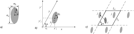
Figure 3: Details of the system studied in this work. (a) Hard-core ellipses with aspect ratio $\kappa={\sigma_{a}}/{\sigma_{b}}$. (b) Skew reference frame used in simulations. Each particle is characterized by two translational and one rotational variable. (c) Simulation box under periodic boundary conditions.

There are $N$ particles in the system. For the sake of generality we use a skew reference frame. Each particle is characterized by three degrees of freedom: two coordinates $x_{i},\ y_{i}$ and one rotation angle $\phi_{i},\ i=1,N$, see figure 3 (b) for illustration. In addition to the skew coordinates, one can also assign Cartesian coordinates $x^{\prime},\ y^{\prime}$ to each particle; the two are related as follows:

$$\left\{\begin{array}[]{c}x^{\prime}=x+y\cos\alpha,\\ y^{\prime}=y\sin\alpha,\\ \end{array}\right.\qquad\left\{\begin{array}[]{c}x=x^{\prime}-y^{\prime}\frac{\cos\alpha}{\sin\alpha},\\ y=y^{\prime}\frac{1}{\sin\alpha}.\\ \end{array}\right.$$ (3.1)

The volume elements of the two coordinates systems are related through the Jacobian of transformation $\mathrm{d}V=\mathrm{d}x^{\prime}\mathrm{d}y^{\prime}=\frac{\partial(x^{\prime},y^{\prime})}{\partial(x,y)}\mathrm{d}x\mathrm{d}y=\sin\alpha\mathrm{d}x\mathrm{d}y$. The particles are placed in a box with sides $L_{x}$ and $L_{y}$ and an angle $\alpha$ between them under periodic boundary conditions, as shown in figure 3 (b)–(c). The skew simulation boxes are designed to accommodate lattices of all possible types. The minimum image convention is applied to compute the interaction energy. As illustrated in figure 3 (c), certain particle $i$ interacts with the closest periodic image of particle $j$. The distance between the two particles is computed as $r_{ij}=\sqrt{x_{ij}^{2}+y_{ij}^{2}+2x_{ij}y_{ij}\cos\alpha}$, where $x_{ij}=x_{i}-x_{j}$ and $y_{ij}=y_{i}-y_{j}$. The usual rule for computing the shortest distance is used: if $x_{ij}>L_{x}/2$, then it is replaced by $x_{ij}-L_{x}$. Similarly, if $x_{ij}<-L_{x}/2$, then it is replaced by $x_{ij}+L_{x}$. The same transformations are applied to the coordinate $y$. The Cartesian coordinates of the vector $\mathrm{d}\vec{r}^{\prime}$ connecting two particles are $\mathrm{d}x^{\prime}=x_{ij}+y_{ij}\cos\alpha$ and $\mathrm{d}y^{\prime}=y_{ij}\sin\alpha$. Together with the rotation angles $\phi_{i}$ and $\phi_{j}$, they are used to determine whether two ellipses overlap [13]. The density of the system is reported in reduced units $\rho=({N}/{V})\ ({1}/{\rho_{\max}})$ where $\rho_{\max}=({2}/{\sqrt{3}})[{1}/({\sigma_{a}\sigma_{b}})]$ is the density of the maximally compact lattice configuration.

3.2 Relative free energy

To measure free energy difference between prospective lattice structures, we use the properly defined order parameters. As discussed in the section 2, one such parameter is $\log(\tau)$, where $\tau=L_{x}/L_{y}$. The ratio of the side lengths is measured directly in simulations and then binned to compute the associated distribution.

Another order parameter that will be utilized is $\alpha$. The rational why the cell angle can be employed as an order parameter is as follows. The system of ellipses can exist either as a fluid or a solid lattice phase, depending on the density [14]. At $\kappa\lesssim 1.5$ [15, 16], ellipses in the solid phase are not aligned with one another, making the so-called plastic lattice [13]. At larger aspect ratios, the particles are aligned similarly to nematic fluids. An example of the simulation cell in which ellipses are aligned is shown in figure 4 (a). The depicted close-packed conformation can be generated from the minimal motif that contains 4 ellipses. It is shown in panel (b) and also highlighted in the right-hand lower corner of the cell. This motif can be obtained from a close-packed configuration of disks by a sequence of unique steps. Let us assume that the diameter of the disks is $\sigma$ and the angle that the left side of the initial box makes with the vertical axis is $\piup/6$, see figure 4 (e). Let us rotate the box counterclockwise by an angle $\gamma$, as shown in figure 4 (d). After that let us stretch the box by the amount $\kappa>1$ in the vertical direction. As a result, disks are transformed into ellipses. The length of the long axis of the ellipses becomes $\kappa\sigma$, as shown in figure 4 (c). Simultaneously, stretching changes the angle that the lower side of the box makes with the horizontal axis, as figure 4 (c) illustrates. While initially it was $\gamma$, now the angle becomes

$$\beta=\cos^{-1}\left(\frac{\cos\gamma}{\sqrt{\cos^{2}\gamma+\kappa^{2}{\sin^{2}\gamma}}}\right).$$ (3.2)

The angle between the left-hand side and the vertical axis also changes. Immediately following the rotation, it is $\piup/6-\gamma$ but after stretching it becomes

$$\lambda=\cos^{-1}\left[\frac{\kappa\cos({\piup}/{6}-\gamma)}{\sqrt{\sin^{2}\left({\piup}/{6}-\gamma\right)+\kappa^{2}{\cos^{2}\left({\piup}/{6}-\gamma\right)}}}\right].$$ (3.3)

As can be seen from figure 4, physically distinct configurations are generated when $\gamma$ changes between 0 and $\piup/6$. All other values lead to redundant configurations. To characterize the state of each ellipse in a specific lattice state, one can use, for instance, the angle that the long axis makes with the horizontal axis, $\phi$. As can be seen from figure 4 (b) $\phi={\piup}/{2}-\beta$. The geometry of the box, on the other hand, can be uniquely specified by its angle $\alpha$ (given that the aspect ratio $\kappa$ is fixed). Both angles, $\phi$ and $\alpha$, are functions of $\gamma$, so there is only one independent variable that fully defines the close-packed structure. All other parameters can be expressed as functions of the chosen variable via relations (3.2) and (3.3). For instance, the rotation angle $\phi$ can be cast as a function of $\alpha$:

$$\phi=F(\alpha;\kappa),$$ (3.4)

where $\kappa$ is the aspect ratio. For the purpose of illustration, figure 4 (e) shows this function for $\kappa=2$, $F_{2}(\alpha)$.

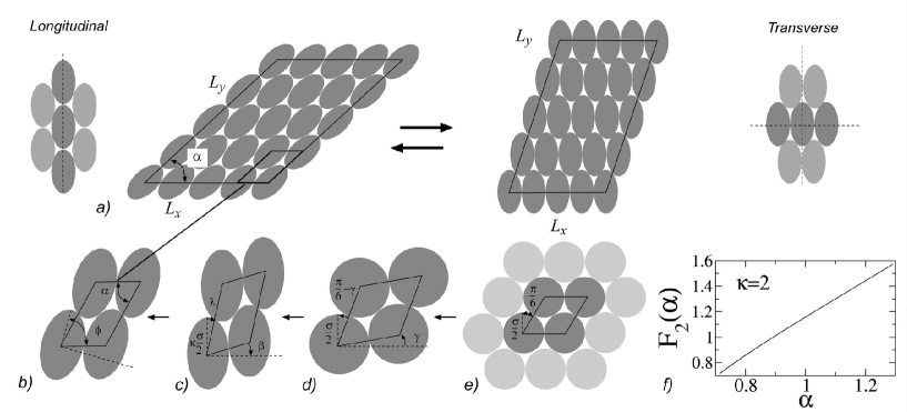
Figure 4: Geometrical details of the simulation cell employed in this study. (a) Geometry of the cell in the longitudinal and transverse lattice states. (b)–(e) A step-wise procedure to establish one-to-one correspondence between the cell angle $\alpha$ and the rotation angle of ellipses $\phi$ in the close-packed configurations. At the first step, e), a minimal non-rectangular box is selected to represent the infinite lattice of hard disks with diameter $\sigma$. At the second step, d), the box is rotated counterclockwise by an angle $\gamma$. At the third step, c), the vertical axis is stretched by the magnitude $\kappa$. At the last step, b), the box is rotated clockwise by the angle $\beta$ necessary to align the lower side with the horizontal axis. Panel e) — dependence of $\phi$ on $\alpha$ for $\kappa$=2.

It can be shown that $\alpha$ varies in the range $\{\alpha_{\rm{min}}=\cos^{-1}[\sqrt{{3}/({3+\kappa^{2}})}],\ \alpha_{\rm{max}}={\piup}/{2}-\cos^{-1}[\sqrt{{3\kappa^{2}\ }/({3+\kappa^{2}})}]\}$, while the corresponding limits of the rotation angle $\phi$ are $\{\phi_{\rm{min}}={\piup}/{2}-\cos^{-1}[\sqrt{{3\ }/({3+\kappa^{2}})}],\ \phi_{\rm{max}}={\piup}/{2}\}$. As $\alpha$ changes, the structure of the lattice changes with it, creating the manifold of an infinite number of lattices differing from one another by the rotation angle $\phi$. This is in contrast to the system of disks, which makes a single hexagonal lattice at high densities. As will become clear below, the lattice types corresponding to the extreme points have a special meaning. At $\alpha=\alpha_{\rm{min}}$, see figure 4 (a), the lattice can be viewed as being assembled from vertical lines of ellipses that make contact with one another through the pole at the short side of the particle. The ellipses are aligned along the line connecting their centers. Consequently, the corresponding lattice type is termed longitudinal (L). The lattice observed at $\alpha=\alpha_{\rm{max}}$ can be assembled from horizontal lines of ellipses which contact each other through the pole at their long side. The orientation of particles is perpendicular to the line connecting their centers, so the corresponding lattice type is called transverse (T). In simulations, the longitudinal lattice can be transformed into the transverse lattice and vice versa by varying the angle $\alpha$. If $\alpha$ is treated as a variable, the transition will happen spontaneously. The system in this case will sample various types of lattices in the course of a single simulation, thereby enabling the computation of their statistical weight. A major difficulty associated with this approach is convergence. To collect sufficient statistics for the distribution function $P(\alpha)$, the system should visit different lattice types a large number of times, which may be difficult if the free energy difference between the concerned lattices is large. To improve the convergence, in this study we employ the method of umbrella sampling [17]. The range $[\alpha_{\rm{min}},\alpha_{\rm{max}}]$ is broken equidistantly into a number of bins, or windows, each assigned a distinct value of $\alpha$. Harmonic potential is applied to bias sampling in simulations to the vicinity of each window. The unbiased distribution $P(\alpha)$ is reconstructed by collecting information on $\alpha$ sampled in all windows. The order parameter relevant for the cell angle is $\log(\sin\alpha)$.

3.3 Method of Einstein crystal

We also compute free energy differences by the method of Einstein crystal (EC) [18, 19]. The key idea of this method is to obtain free energy of the lattice states of interest relative to a common reference state. The free energy of the reference state then drops when the free energy difference is taken. The reference state is modelled by the harmonic Hamiltonian $U_{\rm H}$. Free energy with respect to this model is computed by thermodynamic integration with the help of a coupling constant $\lambda$. How this scheme works in skew coordinates is described in detail in the Appendix. The main formula we use to compute the free energy difference between lattice states characterized by different $\alpha$’s is:

$$\Delta F(\alpha)=-kT(N-1)\log(\sin\alpha)+{\displaystyle\int_{0}^{1}}\langle\Delta U\rangle_{\lambda}\mathrm{d}\lambda.$$ (3.5)

Here, $\langle\Delta U\rangle_{\lambda}$ is the average of the potential energy difference $\Delta U=U_{\rm{HS}}-U_{\rm H}$ computed in simulations driven by the “hybrid” Hamiltonian $U(\lambda)=U_{\rm H}+\lambda\Delta U$. The actual potential energy of the hard-ellipse system is $U_{\rm{HS}}$ and the simulations are performed at a fixed volume $V$ and cell angle $\alpha$ in the reference frame associated with the center of mass. As $\lambda$ is varied between 0 and 1, the Hamiltonian $U(\lambda)$ is transformed from $U_{\rm H}$ to $U_{\rm{HS}}$. As the harmonic potential gradually becomes weaker, the integral in equation (3.5) reports on the spatial extent by which the system is allowed to deviate from the initial configuration, thus providing a measure of the configurational freedom.

The reference Hamiltonian

$$U_{\rm H}=\displaystyle\sum_{i=1}^{N}\left\{\frac{\gamma_{T}}{2}\left[(x_{i}-x_{i}^{0})^{2}+(y_{i}-y_{i}^{0})^{2}\right]+\frac{\gamma_{R}}{2}(\phi_{i}-\phi_{i}^{0})^{2}\right\}$$

contains a set of coordinates $x_{i}^{0},y_{i}^{0},~{}i=1,N$ with respect to which the free energy is evaluated. As a reference we chose a lattice configuration $x_{i}^{0}=(j-0.5)L^{E}_{x}/n,j=1,n$ and $y_{i}^{0}=(k-0.5)L^{E}_{y}/n,\ k=1,n$; ${i=\sum_{j^{\prime}=1}^{j}\sum_{k^{\prime}=1}^{k}}1$, $n\times n=N$. Here, $L^{E}_{x}$ and $L^{E}_{y}$ are the dimensions of the simulation cell in $x$ and $y$ direction, $\phi_{i}^{0}$ are initial angles and $\gamma_{T}$ and $\gamma_{R}$ are adjustable spring constants. It is easy to show that ${N}/{\rho}=\tau{L^{E}_{y}}^{2}\sin\alpha$, where $\tau={L^{E}_{x}}/{L^{E}_{y}}$ is the ratio of the $x$ and $y$ dimensions. Thus, $L^{E}_{y}$ is uniquely defined by $N$, $\rho$, $\alpha$ and $\tau$. Parameter $\tau$ was extracted from constant-volume simulations as the average over all sampled cell side ratios. The integral in equation (3.5) was evaluated by numerical quadrature. In order to reduce the variation seen in $\langle\Delta U\rangle_{\lambda}$, a non-uniform transformation $\zeta(\lambda)$ was applied before integration. A total of 33 grid points, $\zeta_{i},i=1,33$, were generated non-uniformly between $\zeta(0)$ and $\zeta(1)$. The points were chosen so as to maintain a constant level of the numerical integration error, which, after optimization, we judge to be negligible. The statistical error was estimated by performing 5 independent measurements for each state point from which standard deviation was extracted.

3.4 Numerical details

The performed MCVS simulations consist of two types of moves. The first type is the regular MC steps in which particles are randomly displaced and rotated. The maximum magnitude of these steps are adjusted to achieve greater than 30% acceptance. The second type of moves are changes of geometry. They are attempted randomly with 10% overall probability. Box lengths and box angle are updated as described in the previous section. Parameters of these moves are adjusted to achieve greater than 50% acceptance rate. Changes of box lengths are accompanied with the appropriate scaling of particle coordinates. The algorithm of Vieillard-Baron [13] is used to determine if two ellipses overlap.

To perform the umbrella sampling simulations, the range [$\alpha_{\rm{min}}$,$\ \alpha_{\rm{max}}$] was divided equidistantly into 50 windows,$\ \alpha_{i}=\alpha_{\rm{min}}+\Delta(i-1),\ \ \Delta=({\alpha_{\rm{max}}-\alpha_{\rm{min}}})/{49},\ i=1,50$. Simulations were performed in each window with an additional harmonic potential $U_{h}=\frac{1}{2}\epsilon\left(\alpha-\alpha_{i}\right)^{2}$ applied. The strength of the potential $\epsilon$ was set such that the adequate overlap of the histograms at the neighboring windows was achieved. The unbiased distribution $P_{V}(\alpha)$ was obtained at the end of the simulations by the multiple-histogram reweighting method [20, 21].

4 Results

We test the proposed algorithm in simulations of the system of hard-core ellipses. For the sake of comparison, we consider the scheme in which $\tau$ is sampled uniformly, i.e., the $\tau$-sampling algorithm, in addition to the proper 1$/\tau$ sampling law. It is found that proper sampling is essential when the parameter controlling the geometry of the cell varies in a wide range. In other cases, different sampling methods lead to indistinguishable results.

4.1 Solid plastic phase

The first test was performed for a system with $\kappa=1.2$. We used rectangular boxes and set the density at $\rho=0.83$ which is high enough to trigger the transition into the crystalline state yet low enough to preclude aligning of the ellipses. Under these conditions, the system makes the so-called plastic lattice in which particles occupy lattice sites but are capable of rotating by all 180 degrees. A time trace of $\tau$ observed in simulations of this system is shown in figure 5 (a). The aspect ratio varies in the range $[1.0,1.3]$ around an average of ~1.15. At all times, the system occupies a lattice configuration with the distance between neighboring sites $1.17\sigma_{b}$ while the ellipses are capable of adopting any angle $0<\phi<\piup$. A cartoon representation of this structure and its pair distribution function computed for the centers of the ellipses are shown in figure 5 (f) and figure 5 (e), respectively. The lack of alignment between particles is immediately apparent.

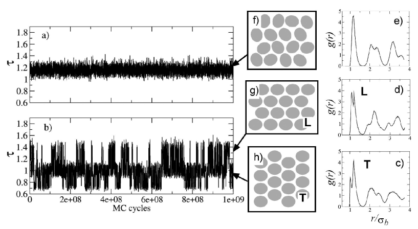
Figure 5: Time traces of the aspect ratio $\tau$ obtained for models with $\kappa=1.2$ in which a) ellipses have different rotation angles and b) — the same rotation angle. Panels f), g) and h) show cartoon representation of lattices in which ellipses are not aligned, or are aligned in the longitudinal (L) and transverse (T) structures, respectively. The pair distribution functions corresponding to these lattices are shown in panels e), d) and c).

We find that the alignment (or rotational degrees of freedom more generally) plays a critical role in determining the structure of the lattice. When it is introduced manually by constraint $\phi_{i}=\phi,\ i=1,N$ where $\phi$ is the common angle of all particles which is allowed to change, the lattice splits into two sub-lattices with a distinct structure. One sub-lattice displays contacts between neighboring ellipses going through the pole at the long side and can be recognized as the transverse lattice. A cartoon representation of this lattice is shown in figure 5 (h). The second sub-lattice is the longitudinal lattice, exhibiting closest contacts between the neighboring ellipses going through their short side, as illustrated in figure 5 (g). All other lattice configurations correspond to free energy maxima and are not directly observable. It is not clear if this is a genuine property of the system or an artifact resulting from the use of rectangular box geometry, suppressing all structures other than the mentioned two. For the demonstration purposes, we considered a small system consisting of $N=16$ particles making $4\times 4$ lattice, so as to enable spontaneous T-L transitions. The time trace of $\tau$ obtained in simulations of this system is shown in figure 5 (b). It is seen that $\tau$ changes in a discontinuous manner among four different values, indicating that the geometry of the box is specific to the lattice type that it contains and suggesting that the aspect ratio can be used as a structural parameter to distinguish between T and L states. Pair distribution functions $g(r)$ obtained for each lattice type, shown in figures 5 (c), (d), demonstrate that the two lattices have a noticeably different structure. The most obvious differences concern the first coordination shell. Compared to the model with full particle rotations, $g(r)$ in the T and L states is split into two sub-maxima. The position of the first sub-maximum in T conformations is at $1.01\sigma_{b}$ while in L conformations it is at $1.1\sigma_{b}$, demonstrating that the particles in the transverse arrangement are capable of approaching each other at shorter distances. This is understandable, given how ellipses are stacked in the two structures, see figure 5 (g) and (h). The second sub-maximum appears at $1.2\sigma_{b}$ in both states. The second and third coordinate shells also show significant differences between T and L conformations.

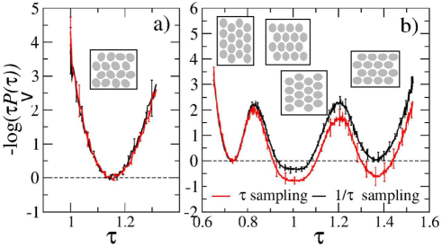
Figure 6: (Colour online) Free energy profile obtained for ellipses with $\kappa=1.2$ in simulations where particles have full rotational freedom, a), and where particle rotation angles are rigidly coupled, b). Minima seen for the constrained system correspond to various stable structures consistent with particular $\tau$ such as transverse and longitudinal states. The results of two sampling methods are as labeled. The $\tau$-sampling method is seen to shift artificially the balance in the statistical weight toward wider boxes. Error bars were estimated from 5 independent trajectories.

So how well does the proposed algorithm reproduce the statistics of the different conformational states? Figure 6 shows the free energy profile $\beta F(\tau)=-\log[\tau P_{V}(\tau)]$ obtained for the system where all particles are free to rotate — panel a), and for the rotationally-constrained system — panel b). As can be expected from figure 5, a single minimum is seen for the unconstrained system and four minima are present for the constrained one. The specific aspect ratios of the minima are $\tau=0.7$, $0.95$, $1.05$ and $1.4$. The two extreme values, $0.7$ and $1.4\approx 1/0.7$, correspond to the longitudinal state. The two minima in the middle are characteristic of the transverse state; they appear to merge in the graph because of being closely spaced. Conformations with $\tau=0.95$ and $1.05$, and those with $\tau=0.7$ and $1.4$, are related by a 90-degree rotation of the reference frame (note that no such transformation ever takes place in the simulations). Corresponding to the same state, they should exhibit the same free energy. It is a crucial test for the algorithm to reproduce this behavior. It is seen from figure 6 (b) that $\beta F(0.95)=\beta F(1.05)$ and $\beta F(0.7)=\beta F(1.4)$ within the error bars, so the proposed $1/\tau$ algorithm successfully passes the test. By contrast, the $\tau$-sampling algorithm predicts that $\beta F(0.95)=\beta F(1.05)$ but $\beta F(1.4)<\beta F(0.7)$ and the difference is statistically significant. The greater population of $\tau=1.4$ state can be explained by the greater statistical weight assigned to conformations with larger $\tau$ by an algorithm in which the sampling probability is flat compared to the case when it declines with $\tau$. Furthermore, even though the $\tau$-sampling method generates the same free energy for $\tau=0.95$ and $1.05$, the value it predicts is twice as large as that of the proper algorithm. Again, the difference is statistically meaningful, which leads us to the conclusion that this method is not capable of reproducing accurately the inter-state statistics for the constrained model under the considered conditions.

By contrast, figure 6 (a) shows that both sampling algorithms lead to the same results, within error bars, for the unconstrained system. It follows, therefore, that the performance of geometry sampling algorithms strongly depends on the system under study, more specifically on the range in which the geometry parameter is varied. If the range is narrow, as in figure 6 (a), the use of the proper algorithm does not make much difference. The average $\tau$ and the shape of the distribution function are generally well reproduced. The algorithm matters, however, when $\tau$ changes in a wide range, as shown in figure 6 (b). Improper sampling leads to significant distortions in $P_{V}(\tau)$ that may ultimately affect the free energy estimates.

4.2 Free energy difference between distinct lattice types

When $\kappa$ is increased beyond ~1.5, the ellipses in the crystalline state become aligned [15, 16]. What is the statistical weight of lattice types with different ellipse orientations? To find that out, we considered the system with $\kappa=4$. The cell angle $\alpha$ for this system varies in the range [0.41, 1.43], which is much wider than the range [0.96, 1.12] appropriate for $\kappa=1.2$. This improves the chances of observing a quantitative difference between the results of using different sampling methods. We considered the cells with 6 rows and 6 columns of ellipses because smaller systems failed to produce stable lattices. Since spontaneous transitions among different lattice types were not observed for the considered system, we had to employ umbrella sampling method to compute the distribution function of the structural order parameter $\alpha$. The details are provided in the section 3. The density of the system was set at $\rho=0.95$ which is much higher than the density of the fluid-solid transition.

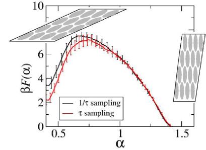
Figure 7: (Colour online) Free energy profile obtained for ellipses with $\kappa=4$. Cartoons show longitudinal and transverse states corresponding to the two minima. Results of the two sampling methods are as labeled.

Free energy profile $\beta F(\alpha)=-\log\left[P_{V}(\alpha)\frac{\sin\alpha}{\cos\alpha}\right]$ obtained in simulations using the proposed sampling algorithm is shown in figure 7 by black line. It has two minima with the lowest free energy corresponding to the transverse and longitudinal states. This agrees with our results for the constrained model of $\kappa=1.2$, suggesting that the presence of two identified stable states is not an artifact of the used cell geometry. The free energy of the longitudinal state is $\beta\Delta F=3.5\pm 0.5$ higher than that of the transverse state. The corresponding figure obtained by the $\tau$-sampling method is $\beta\Delta F=2.2\pm 0.4$. It is seen that this method assigns additional statistical weight to the longitudinal state with smaller $\alpha$. This is in line with our observation from the previous section where we saw states with larger $\tau$ experiencing more frequent sampling. Indeed, since $\sin\alpha={V}/{\tau L_{y}^{2}}$, more sampling for large $\tau$ means more sampling for small $\sin\alpha$ and, by extension, small $\alpha$.

Free energy difference between the L and T states was also evaluated by the EC method. The geometry of the cell was determined in simulations using $1/\tau$ sampling. For the longitudinal structure we used $\alpha=\phi^{0}=\alpha_{\rm{min}}=0.43$ and $\tau=0.558$. For the transverse state, the corresponding numbers were $\alpha=\alpha_{\rm{max}}=1.43$, $\tau=0.288$ and $\phi^{0}=\piup/2$. The initial ellipse orientations $\phi^{0}$ were generated by $F_{4}(\alpha)$ for both structures. Upon combining the results of 5 independent measurements, the free energy difference was evaluated as $\beta\Delta F=3.2\pm 0.2$. This number is in excellent numerical agreement with the prediction made in the $1/\tau$ sampling simulations, $3.5\pm 0.5$, providing an essential validation for this method. By contrast, the $\tau$-sampling algorithm generates an incorrect free energy, $2.2\pm 0.4$, and the error is statistically significant. Based on these observations, we conclude that the use of the proper sampling algorithm is essential for the studied system.

The free energy of the transverse state appears to be lower than that of the longitudinal state. This could be a genuine physical effect stemming from conformational preferences of different lattice configurations. Alternatively, the difference could be a by-product of the small size of the simulation cell. Simulations designed to extract free energy difference as a function of $N$ could help to resolve this ambiguity. Linear segments in $\beta\Delta F(N)$ at large $N$ would indicate genuine free energy difference between the two lattice states. Any other dependence would signal finite-size artifacts. Which of these two scenarios takes place needs to be answered in careful finite-size scaling studies.

5 Conclusions

We introduced an algorithm to perform MC simulations of crystalline systems in boxes with fixed volume but variable shape. Tests performed for the system of hard-core ellipses showed that the performance of the algorithm depends on the range in which the geometrical parameter characterizing the shape varies. If the range is narrow, which is probably the case for the majority of crystalline simulations, the use of the algorithm does not make much difference in comparison with other ad hoc sampling schemes. For wide ranges of the parameters, however, the use of the algorithm may be crucial. In the example of structural transition between transverse and longitudinal lattices, we find that the error in the free energy difference due to the inadequate sampling method reaches 40%. How large it may become, and how wide the corresponding variation range should be, will depend on the system of interest. However, as a general rule, the error due to the incorrect sampling should not be simply neglected.

At the same time, we note that the magnitude of the error declines when the range of the sampled parameter becomes narrower. This will happen, among other reasons, when the number of particles $N$ increases. Thus, proper finite-size analysis, in addition to yielding important information about the scaling properties of the studied system, will also help to combat the errors associated with the inadequate methods of sampling simulation box shapes.

Appendix

A.1 Algorithm for the three-dimensional space

It is possible to conduct constant-volume simulations with the changing shape in the three-dimensional space. Let us assume that the geometry of the box is defined by six variables, three lengths $L_{x},L_{y}$ and $L_{z}$, and three angles $\alpha,\beta$ and $\gamma$, as shown in figure A.1. Let us further assume for now that the box is rectangular, $\alpha=\beta=\gamma=\piup/2$. The analogue of the constant-pressure distribution (2.3) in 3D will be a function of the lengths of the box:

$$P\left(L_{x},L_{y},L_{z}\right)\sim\mathrm{e}^{-\beta{\mathcal{P}}L_{x}L_{y}L_{z}}\ Q(N,T,L_{x}L_{y}L_{z};\tau).$$ (A.1)

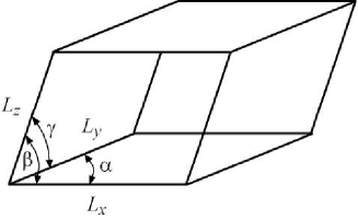
Figure A.1: Simulation box in 3D is defined by three variables: three box lengths $L_{x}$, $L_{y}$ and $L_{z}$, and three angles $\alpha$, $\beta$ and $\gamma$.

Aspect ratios can be computed for all three sides of the box lying in $xy$, $xz$ and $zy$ planes. We will try to change only one $\tau$ at a time. The corresponding distribution function, for instance for $\tau=L_{x}/L_{y}$, can be computed as follows:

$$P_{V}(\tau)\sim\ \int{\mathrm{d}L_{x}\mathrm{d}L_{y}\mathrm{d}L_{z}\delta\left(V-L_{x}L_{y}L_{z}\right)\delta(\tau-L_{x}/L_{y})}\mathrm{e}^{-\beta{\mathcal{P}}L_{x}L_{y}L_{z}}\ Q(N,T,L_{x}L_{y}L_{z};L_{x}/L_{y}).$$ (A.2)

By making the substitution $y=L_{x}L_{y}L_{z}$ one can eliminate the integral over $L_{z}$ obtaining:

$$P_{V}(\tau)\sim\ \int{\mathrm{d}L_{x}\mathrm{d}L_{y}\frac{1}{L_{x}L_{y}}\ \delta(\tau-L_{x}/L_{y})}\mathrm{e}^{-\beta{\mathcal{P}}V}\ Q(N,T,V;L_{x}/L_{y}).$$

After the second substitution $y=L_{x}{/L}_{y}$ and elimination of $L_{x}$, one arrives at:

$$P_{V}(\tau)\sim\ \mathrm{e}^{-\beta{\mathcal{P}}V}\int{\mathrm{d}L_{y}\frac{1}{L_{y}}}\frac{1}{\tau}Q(N,T,V;\tau)\sim\ \frac{1}{\tau}Q(N,T,V;\tau).$$

This result does not depend on the integration order. Therefore, we find that the sampling law in three-dimensional space is the same as in the two-dimensional space.

Since there is no difference with respect to the dimensionality, it is convenient to use the algorithms developed for 2D and apply them to 3D boxes. In particular, the idea of sampling one side of the box and then updating alternatively either another side or the angle between the sides can be reused. The volume of the box with variable angles is

$$V=L_{x}L_{y}L_{z}\sqrt{1-{\cos^{2}\alpha}-{\cos^{2}\beta}-{\cos^{2}\gamma}+2\cos\alpha\cos\beta\cos\gamma}.$$

In MC sampling, one should take alternatively pairs of a side and a second side or a side and an angle until all such combinations are exhausted. If the length $L_{x}$ is updated to $L^{\prime}_{x}$ then companion steps should be updating $L_{y}$ or $\cos\alpha$. The second possible combination is ($L_{x}$, $L_{z})$ or $(L_{x},\ \cos\beta)$. The third and final combination is ($L_{y}$, $L_{z})$ or $(L_{y},\ \cos\gamma)$. Specific formulas for how to update the lengths and angles can be obtained from the condition that the volume of the cell remains constant. If for instance $L_{x}$ is sampled and a trial value is $L^{\prime}_{x}$, then the trial value for the length in the $y$-direction should be $L^{\prime}_{y}=V/L^{\prime}_{x}$ and the trial angle in the $xy$ plane

$$\cos\alpha^{\prime}=\sqrt{\cos\beta\cos\gamma+\sqrt{{\cos^{2}\beta}{\cos^{2}\gamma}+1-{\cos^{2}\beta}-{\cos^{2}\gamma}-{V^{2}}/{{L^{\prime 2}_{x}}L_{y}^{2}L_{z}^{2}}}}.$$

Similar formulas can be obtained for $(L_{x},\ L_{z},\ \cos\beta)$ and $(L_{y},\ L_{z},\cos\gamma)$ combinations by permutations.

A.1.1 Einstein crystal method in skew coordinates

There are certain caveats associated with the use of EC method in conjunction with the skew coordinates, which we explain below. To evaluate the Hamiltonian, we need momenta in addition to the coordinates. These can be obtained using a general formula $P_{x}={\mathrm{d}K}/{\mathrm{d}\dot{x}}$, where $x$ is the coordinate, $\dot{x}$ is the time derivative of the coordinate and $K$ is the kinetic energy. For Cartesian coordinates, the kinetic energy is known: $K=\frac{m}{2}({\dot{x}}^{\prime 2}+{\dot{y}}^{\prime 2})$, where $m$ is the mass of the particle. It yields the familiar momenta $P_{x}^{\prime}=m{\dot{x}}^{\prime}$ and $P_{y}^{\prime}=m{\dot{y}}^{\prime}$. Assuming that skew and Cartesian coordinates are related by expression (3.1) it follows that

$$K=\frac{m}{2}({\dot{x}}^{2}+{\dot{y}}^{2}+2{\dot{x}}{\dot{y}}\cos\alpha),$$ (A.3)

thus, one can find the skew momenta: $P_{x}={\mathrm{d}K}/{\mathrm{d}\dot{x}}=m(\dot{x}+\dot{y}\cos\alpha)=P_{x}^{\prime}$ and $P_{y}=m(\dot{y}+\dot{x}\cos\alpha)=P_{x}^{\prime}\cos\alpha+P_{y}^{\prime}\sin\alpha$. The reverse transformation $P_{x}^{\prime}=P_{x}$ and $P_{y}^{\prime}=\frac{1}{\sin\alpha}(P_{y}-P_{x}\cos\alpha)$ allows one to compute the Jacobian: $\displaystyle{\partial(P_{x}^{\prime},P_{y}^{\prime})}/{\partial P_{x},P_{y}}={1}/{\sin\alpha}$ leading to the volume element $\mathrm{d}P_{x}^{\prime}\mathrm{d}P_{y}^{\prime}=\frac{1}{\sin\alpha}\mathrm{d}P_{x}\mathrm{d}P_{y}$. The kinetic energy

$$K=\frac{1}{2m}\frac{1}{\sin^{2}\alpha}(P_{x}^{2}+P_{y}^{2}-2P_{x}P_{y}\cos\alpha)$$

can be found by expressing time derivatives of the coordinates in terms of the momenta and then substituting the results into equation (A.3).

Now, let us compute the partition function for one particle:

$$Q(N,V,T)=\frac{1}{1!h^{2}}\int{\mathrm{e}^{-\beta H}\mathrm{d}P_{x}^{\prime}\mathrm{d}P_{y}^{\prime}\mathrm{d}x^{\prime}\mathrm{d}y^{\prime}}=\frac{V}{1!h^{2}}\int{\mathrm{e}^{-\beta K}\mathrm{d}P_{x}^{\prime}\mathrm{d}P_{y}^{\prime}\frac{1}{V}\int{\mathrm{e}^{-\beta U}\mathrm{d}x^{\prime}\mathrm{d}y^{\prime}}}=Q_{\rm{id}}\times Q_{\rm{ex}},$$

where we used the property that coordinates and momenta can be partitioned and U is the potential energy of the system. The two integrals in this expression correspond to ideal $Q_{\rm{id}}$ and excess $Q_{\rm{ex}}$ partition functions giving rise to ideal and excess free energy, correspondingly. Let us evaluate the ideal part in the skew reference frame:

$$Q_{\rm{id}} =\frac{V}{1!h^{2}}\int{\mathrm{e}^{-\beta K}\frac{1}{\sin\alpha}\mathrm{d}P_{x}\mathrm{d}P_{y}}$$

$$=\frac{V}{h^{2}}\int{{\rm{exp}}\left\{-\beta\frac{1}{2m}\frac{1}{\sin^{2}\alpha}\left[P_{x}^{2}+P_{y}^{2}-2P_{x}P_{y}\cos\alpha\right]\right\}\frac{1}{\sin\alpha}\mathrm{d}P_{x}\mathrm{d}P_{y}}=\frac{V}{h^{2}}\left(\frac{2\piup m}{\beta}\right),$$

which turns out to be exactly the same as the equivalent expression in the Cartesian coordinates. Extending these calculations to $N$ particles will produce $Q_{\rm{id}}=({1}/{N!})({V^{N}}/{h^{2N}})({2\piup m}/{\beta})^{N}$, which for sufficiently large $N$ will give the familiar expression of the free energy of ideal gas: $\beta F_{\rm{id}}=N[\log(\rho)-\log({1}/{\lambda^{2}})-1]$, where $\lambda=\sqrt{{\beta h^{2}}/{2\piup m}}$. Note that this expression does not depend on $\alpha$, so the ideal part of the free energy can be neglected when working in the skew reference frame if relative free energy is of interest. Moving on to the excess partition function, one finds for one particle:

$$Q_{\rm{ex}}=\frac{1}{V}\int{\mathrm{e}^{-\beta U}\mathrm{d}x^{\prime}\mathrm{d}y^{\prime}}=\frac{\sin\alpha}{V}\int{\mathrm{e}^{-\beta U}\mathrm{d}x\mathrm{d}y}.$$

Generalization to $N$ particles

$$Q_{\rm{ex}}=\frac{\sin^{N}\alpha}{V^{N}}\int{\mathrm{e}^{-\beta U}{\displaystyle\prod_{i}}\mathrm{d}x_{i}\mathrm{d}y_{i}}$$ (A.4)

gives rise to the excess free energy $\beta F_{\rm{ex}}(N,V,T)=-\log{Q_{\rm{ex}}}$, which is fully defined by the interaction energy $U(x_{1},y_{1},...,x_{N},y_{N})$.

Let us focus on the system of hard disks for now, and introduce a scaling constant $\lambda$ that will transform the hard-sphere potential $U_{\rm{HS}}$ into the harmonic potential $U_{\rm H}={\sum_{i=1}^{N}}({\gamma_{T}}/{2})\left[(x_{i}-x_{i}^{0})^{2}+(y_{i}-y_{i}^{0})^{2}\right]$:

$$U(\lambda)=U_{\rm H}(1-\lambda)+\lambda U_{\rm{HS}}=U_{\rm H}+\lambda(U_{\rm{HS}}-U_{\rm H})=U_{\rm H}+\lambda\Delta U,\qquad\Delta U=U_{\rm{HS}}-U_{\rm H}.$$ (A.5)

Here, $x_{i}^{0},y_{i}^{0},~{}i=1,N$ are the positions of the ideal lattice with respect to which the free energy is evaluated. At $\lambda=0$, the system is described by the harmonic potential. It constitutes a set of independent harmonic oscillators with frequency controlled by the spring constant $\gamma_{T}$. At $\lambda=1$, we obtain the system of our interest — hard spheres. The “hybrid” potential $U(\lambda)$ defines some fictitious system which physically makes sense only at the extreme points of $\lambda$. The free energy of that fictitious system $\beta F_{\rm{ex}}(\lambda)=-\log{Q_{\rm{ex}}}$ can be used to compute the free energy difference between the end points: $\Delta F=F_{\rm{ex}}(\lambda=1)-F_{\rm{ex}}(\lambda=0)=F_{\rm{HS}}-F_{\rm H}$. Since $F_{\rm H}$ is known analytically, this formula allows us to compute $F_{\rm{HS}}$ as a sum $F_{\rm{HS}}=F_{H}+\Delta F$, making the evaluation of $\Delta F$ a key task. This task can be accomplished by taking the derivative of $F_{\rm{ex}}(\lambda)$ with respect to $\lambda$:

$$\frac{\mathrm{d}\beta F_{\rm{ex}}(\lambda)}{\mathrm{d}\lambda}=-\frac{1}{Q_{\rm{ex}}(\lambda)}\frac{\mathrm{d}Q_{\rm{ex}}(\lambda)}{\mathrm{d}\lambda}=-\frac{1}{Q_{\rm{ex}}(\lambda)}\frac{\sin^{N}\alpha}{V^{N}}\int\mathrm{e}^{-\beta U(\lambda)}\beta\Delta U\prod\mathrm{d}x_{i}\mathrm{d}y_{i}=\beta\langle\Delta U\rangle_{\lambda},$$ (A.6)

where symbol $\langle...\rangle_{\lambda}$ denotes average in ensemble generated by $U(\lambda)$. After the integration of the derivative, one obtains:

$$\Delta F={\displaystyle\int_{0}^{1}}\frac{\mathrm{d}F_{\rm{ex}}(\lambda)}{\mathrm{d}\lambda}\mathrm{d}\lambda={\displaystyle\int_{0}^{1}}\langle\Delta U\rangle_{\lambda}\mathrm{d}\lambda.$$

This is the key formula which relates the free energy of the system of interest $F_{\rm{HS}}$ to the integral obtained in simulations of the hybrid system:

$$F_{\rm{HS}}=F_{\rm H}+{\displaystyle\int_{0}^{1}}\langle\Delta U\rangle_{\lambda}\mathrm{d}\lambda.$$ (A.7)

Provided that $\gamma_{T}$ is taken sufficiently large, the partition function in harmonic approximation can be evaluated analytically as:

$$Q^{H}_{\rm{ex}}=\frac{\sin^{N}\alpha}{V^{N}}\int{\rm{exp}}\left\{{-\beta\sum\frac{\gamma_{T}}{2}\left[(x_{i}-x_{i}^{0})^{2}+(y_{i}-y_{i}^{0})^{2}\right]}\right\}\prod\mathrm{d}x_{i}\mathrm{d}y_{i}=\frac{\sin^{N}\alpha}{V^{N}}\left(\frac{2\piup}{\beta\gamma_{T}}\right)^{N}.$$

The corresponding free energy then is:

$$F_{H}=-kTN\log\left(\frac{\sin\alpha}{V}\frac{2\piup}{\beta\gamma_{T}}\right)=-kTN\log\left(\frac{2\piup}{V\beta\gamma_{T}}\right)-kTN\log(\sin\alpha),$$

where $k$ is the Boltzmann constant. In this expression, we singled out the second term that depends on $\alpha$. The first term will vanish in calculations of free energy differences using the same $\gamma_{T}$ but different $\alpha$. Thus, the harmonic free energy relevant for our calculations is just $-kTN\log(\sin\alpha)$. The final formula for the free energy becomes:

$$\Delta F=-kTN\log(\sin\alpha)+{\displaystyle\int_{0}^{1}}\langle\Delta U\rangle_{\lambda}\mathrm{d}\lambda.$$ (A.8)

For ellipses, the methodology remains the same except that now we need to add $N$ new degrees of freedom — particle angles. The ideal part of the free energy will get new terms arising from new variables (comprising the inertia tensor of the ellipses) but these are independent of $\alpha$, so they can be neglected. In the excess part, we will get additional integration over the angles with normalization constant $(2\piup)^{N}$. The harmonic potential will now also apply to the angles:

$$U_{\rm H}={\displaystyle\sum_{i=1}^{N}}\left\{\frac{\gamma_{T}}{2}\left[(x_{i}-x_{i}^{0})^{2}+(y_{i}-y_{i}^{0})^{2}\right]+\frac{\gamma_{R}}{2}(\phi_{i}-\phi_{i}^{0})^{2}\right\},$$

where $\gamma_{R}$ is an additional spring constant and $\phi_{i}^{0}$ are the set of initial particle angles. The new partition function changes into:

$$Q^{H}_{\rm{ex}}=\frac{\sin^{N}\alpha}{V^{N}(2\piup)^{N}}\left(\frac{2\piup}{\beta\gamma_{T}}\right)^{N}\left(\frac{2\piup}{\beta\gamma_{R}}\right)^{N/2}$$

but the free energy part that depends on $\alpha$ remains the same: $-kTN\log(\sin\alpha)$.

In the course of simulations, we discovered that the integrand $\langle\Delta U\rangle_{\lambda}$ in formula (A.8) converges very inefficiently for $\lambda=1$, which corresponds to the system driven by the hard-core potential while its potential energy is evaluated with the help of the harmonic potential. The potential energy in this case experiences strong fluctuations that decay very slowly over time. After some research, the slow convergence was tracked down to the movements of the simulation cell as a whole. Since the random displacements of the particles during MC steps are uncorrelated, the center of mass of the system experiences displacements from its initial position as well. These displacements average out over time because of the law of large numbers but it may take a long simulation time in order to see that. For non-zero $\lambda$’s, the collective movements of all particles are not an issue because the harmonic potential suppresses large-scale deviations from the initial coordinates. At the same time, the displacements of all particles as a whole do not create a physically distinct state and thus should not affect the relative free energy. It, therefore, makes sense to transition to the reference frame associated with the center of mass of the system. The description then includes the coordinates of the center of mass $x_{c}$, $y_{c}$ and $N-1$ coordinates of the particles which characterize their mutual arrangement (conformations) (the coordinates of the remaining particle are expressed in terms of these new variables). Under periodic boundary conditions, the center of mass samples from the volume $V/N$, where $V$ is the total volume of the system. This is the quantity that will appear in front of the integral (A.4) when the integration is carried out over $x_{c}$ and $y_{c}$. Importantly, this volume per particle is the same for all $\alpha$, so the associated term of free energy will drop when the difference is taken. Integration over the remaining $N-1$ coordinates yields:

$$Q^{H}_{\rm{ex}}=\frac{\sin^{N-1}\alpha}{V^{N-1}(2\piup)^{N}}\left(\frac{2\piup}{\beta\gamma_{T}}\right)^{N-1}\left(\frac{2\piup}{\beta\gamma_{R}}\right)^{N/2}$$

with the relevant $\alpha$-dependent term of free energy $-kT(N-1)\log(\sin\alpha)$. This leads to the final expression (3.5) for the free energy given in the section 3. The function $\langle\Delta U\rangle_{\lambda}$ is evaluated in simulations carried out in the reference frame of the center of mass. In practice, this was achieved by aligning the coordinates of the center of mass at each MC step. We found that this can be accomplished by keeping track of two sets of coordinates: one containing real coordinates and the other storing coordinates that are periodically imaged. This prevented discontinuous jumps of the center of mass position when particles were put back into the simulation cell by the boundary conditions. We found that formula (3.5) produces the same free energy difference as formula (A.8) but at a much lower computational cost. For systems with $N>100$, formula (A.8) could not be converged at all. We emphasize that formula (3.5) applies only when $\gamma_{T}$ and $\gamma_{R}$ are taken to be the same for different $\alpha$’s. Additionally, they should be sufficiently large, so that analytical integration in the partition function applies. In practice, this can be achieved by gradually increasing $\gamma_{T}$ and $\gamma_{R}$ while monitoring $\langle\Delta U\rangle_{\lambda}$ at $\lambda=0$. The point at which this function becomes equal to the energy of the harmonic approximation $\frac{1}{2}kTN_{F}$ indicates that the spring constants are strong enough. Here, $N_{F}$ is the number of degrees of freedom in the system. For the model where all particles are allowed to rotate $N_{F}=2N-2+N=3N-2$ and for the model with coupled rotations $N_{F}=2N-2+1=2N-1$.

Integration of $\langle\Delta U\rangle_{\lambda}$ was carried out numerically. To counter a very strong decline of $\langle\Delta U\rangle_{\lambda}$ in the limit of $\lambda\to 1$, the following change of variables was performed:

$$\left\{\begin{array}[]{c}\zeta=\frac{a_{t}}{b_{t}-1}\frac{1}{(1+\alpha_{t}-\lambda)^{b_{t}-1}},\\ \lambda=1+\alpha_{t}-(\frac{a_{t}}{b_{t}-1}\frac{1}{\zeta})^{{1}/{(b_{t}-1)}}.\\ \end{array}\right.$$ (A.9)

The integral in equation (3.5) was transformed accordingly:

$$\int_{0}^{1}{\langle\Delta U\rangle_{\lambda}}\mathrm{d}\lambda=\int_{\zeta(0)}^{\zeta(1)}{\langle\Delta U\rangle_{\zeta}}\frac{1}{a_{t}}\left(\frac{a_{t}}{b_{t}-1}\frac{1}{\zeta}\right)^{{b_{t}}/{(b_{t}-1)}}\mathrm{d}\zeta=\int_{\zeta(0)}^{\zeta(1)}{F(\zeta)\mathrm{d}\zeta},$$ (A.10)

where parameters $a_{t}=1287.4$ and $b_{t}=0.44708$ were determined by fitting. The constant $\alpha_{t}$ was set equal $10^{-6}$.

Both $\langle\Delta U\rangle_{\zeta}$ and the derivative of this function $\frac{\mathrm{d}\langle\Delta U\rangle_{\zeta}}{\mathrm{d}\zeta}$ were used to compute the integral. The latter can be extracted directly from simulations through the following relationship:

$$\frac{\mathrm{d}\langle\Delta U\rangle_{\zeta}}{\mathrm{d}\zeta}=-\beta(\langle\Delta U^{2}\rangle_{\zeta}-\langle\Delta U\rangle_{\zeta}^{2}).$$

The derivative of the integrand in equation (A.10) can be found as

$$F^{\prime}(\zeta)=\frac{\mathrm{d}\langle\Delta U\rangle_{\zeta}}{\mathrm{d}\zeta}\frac{1}{a_{t}}\left(\frac{a_{t}}{b_{t}-1}\frac{1}{\zeta}\right)^{{b_{t}}/{(b_{t}-1)}}-\frac{b_{t}}{a_{t}^{2}}\left(\frac{a_{t}}{b_{t}-1}\frac{1}{\zeta}\right)^{{(2b_{t}-1)}/{(b_{t}-1)}}\langle\Delta U\rangle_{\zeta}.$$

Numerical integration was carried out by the Euler–Maclaurin method [22]. Initially, there were 15 non-overlapping segments considered with widths adjusted iteratively to achieve $\Delta\zeta_{i}=\zeta_{i+1}-\zeta_{i}\sim{1}/{|F(\zeta_{i})|},\ i=0,14$. This allowed us to make the numerical error almost uniform across the integration range. Each segment was integrated using the 2-point formula $P_{2}=h({f_{1}}/{2}+{f_{2}}/{2})+{h^{2}}(p_{1}-p_{2})/{12}$, where $h=\zeta_{2}-\zeta_{1}$, $f_{1}$ and $p_{1}$ are the values of the integrand and its first derivative at the first point of the segment and $f_{2}$ and $p_{2}$ are the corresponding quantities at the second point of the segment. Each segment was then split evenly in two, yielding an intermediate point $\zeta^{\prime}=\frac{1}{2}(\zeta_{1}+\zeta_{2})$, and integration was repeated using the 3-point formula $P_{3}=h({f_{1}}/{2}+f^{\prime}+{f_{2}}/{2})+{h^{2}}(p_{1}-p_{2})/{12}$, where $f^{\prime}$ is the value of the function at $\zeta^{\prime}$ and $h=\frac{1}{2}(\zeta_{2}-\zeta_{1})$. Since the Euler–Maclaurin formula is accurate up to $O(h^{4})$, the two estimates, $I=P_{2}+\alpha^{\prime}h^{4}$ and $I=P_{3}+\frac{1}{16}\alpha^{\prime}h^{4}$ can be combined in a Romberg-style procedure to yield a better approximation for the integral $I={(16P_{3}-P_{2})}/{15}$, which is accurate up to terms $O(h^{6})$. The error contained in this estimate can be approximated by ${(P_{3}-P_{2})}/{15}$, which is the error of the 3-point integration formula. If the error estimated in this way turned out to be higher than a pre-set target value, we continued to split the concerned segments until a desired accuracy was reached. A total of 33 integration points were generated in this manner. The grid was much denser for $\zeta$ points corresponding to $\lambda\sim 1$. The estimated integration error is less than 0.1% in relative terms. For the free energy difference, this translates into a 3% numerical error, which is about twice as low as the statistical error resulting from incomplete sampling.

Ukrainian 0

Äî àëãîðèòìó ïðîâåäåííÿ Ìîíòå Êàðëî ñèìóëÿöié â êîìiðêàõ ìîäåëþâàííÿ ç ïîñòiéíèì îá’єìîì òà çìiííîþ ôîðìîþ À. Áàóìêåòíåð

             
Iíñòèòóò ôiçèêè êîíäåíñîâàíèõ ñèñòåì ÍÀÍ Óêðà¿íè, âóë. Ñâєíöiöüêîãî, 1, 79011, Ëüâiâ, Óêðà¿íà

References

- [1] van Gunsteren W. F., Dolenc J., Biochem. Soc. Trans., 2008, 36, 11, doi:10.1042/BST0360011.
- [2] Frenkel D., Smit B., Understanding Molecular Simulation, Academic Press, San Diego, 2002.
- [3] Panagiotopoulos A. Z., In: Observation, Prediction and Simulation of Phase Transitions in Complex Fluids, Vol. 460, Baus M., Rull L. F., Ryckaert J. P. (Eds.), Springer, Dordrecht, 1995, 463–501, doi:10.1007/978-94-011-0065-6_11.
- [4] Hukushima K., Nemoto K., J. Phys. Soc. Jpn., 1996, 65, No. 6, 1604, doi:10.1143/JPSJ.65.1604.
- [5] Swendsen R. H., Wang J. S., Phys. Rev. Lett., 1986, 57, No. 21, 2607, doi:10.1103/PhysRevLett.57.2607.
-
[6]
Tesi M. C., van Rensburg E. J. J., Orlandini E., Whittington S. G., J. Stat. Phys., 1996, 82, 155,
doi:10.1007/BF02189229. - [7] Fortini A., Dijkstra M., J. Phys.: Condens. Matter, 2006, 18, No. 28, L371, doi:10.1088/0953-8984/18/28/L02.
- [8] Noya E. G., Vega C., de Miguel E., J. Chem. Phys., 2008, 128, No. 15, 154507, doi:10.1063/1.2901172.
- [9] Allen M. P., Tildesley D. J., Computer Simulations of Liquids, Oxford University Press, Oxford, 1987.
- [10] Veerman J. A. C., Frenkel D., Phys. Rev. A, 1990, 41, 3237, doi:10.1103/PhysRevA.41.3237.
- [11] Bolhuis P., Frenkel D., J. Chem. Phys., 1997, 106, No. 2, 666, doi:10.1063/1.473404.
- [12] Rodgers J. M., Smit B., J. Chem. Theory Comput., 2012, 8, No. 2, 404, doi:10.1021/ct2007204.
- [13] Vieillard-Baron J., J. Chem. Phys., 1972, 56, No. 10, 4729, doi:10.1063/1.1676946.
- [14] Cuesta J. A., Frenkel D., Phys. Rev. A, 1990, 42, No. 4, 2126, doi:10.1103/PhysRevA.42.2126.
- [15] Bautista-Carbajal G., Odriozola G., J. Chem. Phys., 2014, 140, No. 20, 204502, doi:10.1063/1.4878411.
- [16] Xu W. S., Li Y. W., Sun Z. Y., An L. J., J. Chem. Phys., 2013, 139, No. 2, 024501, doi:10.1063/1.4812361.
- [17] Torrie G. M., Valleau J. P., J. Comput. Phys., 1977, 23, No. 2, 187, doi:10.1016/0021-9991(77)90121-8.
- [18] Frenkel D., Ladd A. J. C., J. Chem. Phys., 1984, 81, No. 7, 3188, doi:10.1063/1.448024.
-
[19]
Khanna V., Anwar J., Frenkel D., Doherty M. F., Peters B., J. Chem. Phys., 2021, 154, No. 16, 164509,
doi:10.1063/5.0044833. - [20] Ferrenberg A. M., Swendsen R. H., Phys. Rev. Lett., 1989, 63, No. 12, 1195, doi:10.1103/PhysRevLett.63.1195.
- [21] Kumar S., Bouzida D., Swendsen R. H., Kollman P. A., Rosenberg J. M., J. Comput. Chem., 1992, 13, No. 8, 1011, doi:10.1002/jcc.540130812.
- [22] DeVries P. L., A First Course in Computational Physics, John Wiley Sons, Inc., 1993.
Ukrainian \adddialect\l@ukrainian0 \l@ukrainian