Nonlinear dynamical topological phases in Cooper-pair box array

Abstract

The topological property of a system is a static property in general. For instance, the topological edge state is observed by measuring the local density of states. In this work we propose a system whose topological property is only revealed by dynamics. As a concrete example, we explore a nonlinear dynamical topological phase transition revealed by a quench dynamics of a Cooper-pair box array connected with capacitors. It is described by coupled nonlinear differential equations due to the Josephson effect. It is trivial as far as the static system is concerned. However, the wave propagation induced by the quench dynamics demonstrates a rich topological phase diagram in terms of the strength of the input.

Topological physics is one of the most extensively studied fields in condensed-matter physics[1, 2]. The notion of topology is also applicable to artificial topological systems such as photonic[3, 4, 5, 6, 7, 8], acoustic[9, 10, 11, 12, 13], mechanical[14, 15, 16, 17, 18, 19, 20, 21] and electric circuit[22, 23, 24, 25, 26, 27] systems. New feature of these artificial topological systems are that nonlinearity is naturally introduced as in photonics[28, 29, 30, 31, 32, 33, 34, 35, 36], mechanics[37, 38, 39] and electric circuits[40, 41, 42]. In particular, electric circuits simulate almost all topological phases. Active topological electric circuits[43] is realized by using nonlinear Chua’s diode circuit. Topological Toda lattice is realized by using variable capacitance diodes[42].

Recently, the development of superconducting qubits is very rapid as a method for quantum computation[44, 45]. The transmon qubit is a successful example of a superconducting qubit[46, 47] based on a Cooper-pair box (CPB)[44, 48, 49] made of the Josephson junction and a capacitor, as shown in Fig.1(a).

In this work we explore a nonlinear topological phase transition in a CPB array connected with capacitors as in Fig.1(d), where alternating capacitances are arranged for the array to acquire a structure akin to that of the one-dimensional Su-Schrieffer-Heeger (SSH) chain. The SSH model is the well-known topological system, where the topological phase is signaled by the emergence of zero-energy topological edge states. They are detected by the measurement of the local density of states. However, the CPB array reveals an unfamiliar feature in topological physics, where the system is trivial as far as the static system is concerned.

To reveal the topological structure, we evoke a dynamical property. We analyze a quench dynamics by giving a flux to the left-end CPB and studying its time evolution. We have found four types of propagations. (i) There are standing waves mainly at the left-end CPB and weakly at a few adjacent odd-number CPBs. Additionally, there are propagating waves into the bulk. (ii) There are only propagating waves spreading into other CPBs. (iii) The standing wave is trapped strictly at the left-end CPB. (iv) The coupled standing waves are trapped to double CPBs at the left-end. These four modes correspond to the topological phase, the trivial phase, the trapped phase and the dimer phase. We determine the phase diagram with the aid of a phase indicator defined by the saturated amplitude. The present model presents a system whose topological property is only revealed by a dynamical method.

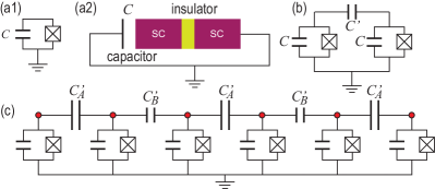
Figure 1: Illustration of (a) a Cooper-pair box, (b) double Cooper-pair boxes connected via a capacitor and (c) a dimerized Cooper-pair box array.

Model: A CPB is an electric circuit made of a Josephson junction and a capacitor with capacitance $C$, as illustrated in Fig.1(a). We investigate a CPB array connected by capacitors shown in Fig.1(c). The Lagrangian is given by

$$\mathcal{L(}\Phi,\dot{\Phi})= \sum_{n}\left[\frac{C_{n}}{2}\dot{\Phi}_{n}^{2}+\frac{I_{\text{c}}\Phi_{0}}{2\pi}\cos 2\pi\frac{\Phi_{n}}{\Phi_{0}}\right]$$

$$+\sum_{n}\frac{C_{n}^{\prime}}{2}(\dot{\Phi}_{n}-\dot{\Phi}_{n+1})^{2},$$ (1)

where $I_{\text{c}}$ is the critical current of the Josephson junction, $\Phi_{0}\equiv h/2e$ is the unit flux, $C_{n}$ is the capacitance in the $n$-th CPB, and $\Phi_{n}$ is a magnetic flux across the $n$-th Josephson junction. The first line describes the $n$-th CPB, and the second line describes the coupling between the $n$-th and ($n+1$)-th CPBs via the capacitance $C_{n}^{\prime}$. It is summarized as

$$\mathcal{L(}\Phi,\dot{\Phi})=\frac{1}{2}\sum_{n,m}M_{nm}\dot{\Phi}_{n}\dot{\Phi}_{m}+\sum_{n}\frac{I_{\text{c}}\Phi_{0}}{2\pi}\cos 2\pi\frac{\Phi_{n}}{\Phi_{0}},$$ (2)

where

$$M_{nm}=[C_{n}+C_{n}^{\prime}+C_{n-1}^{\prime}]\delta_{nm}-[C_{n}^{\prime}\delta_{m,n+1}+C_{m}^{\prime}\delta_{n,m+1}],$$ (3)

with $C_{0}^{\prime}=0$. The Euler-Lagrange equation reads

$$\sum_{m}M_{nm}\ddot{\Phi}_{m}+I_{\text{c}}\sin 2\pi\frac{\Phi_{n}}{\Phi_{0}}=0.$$ (4)

The canonical conjugate of the flux $\Phi_{n}=\partial\mathcal{L}/\partial\dot{\Phi}_{n}$ is the charge acquired in the capacitor, and given by

$$Q_{n}=M_{nm}\dot{\Phi}_{m}.$$ (5)

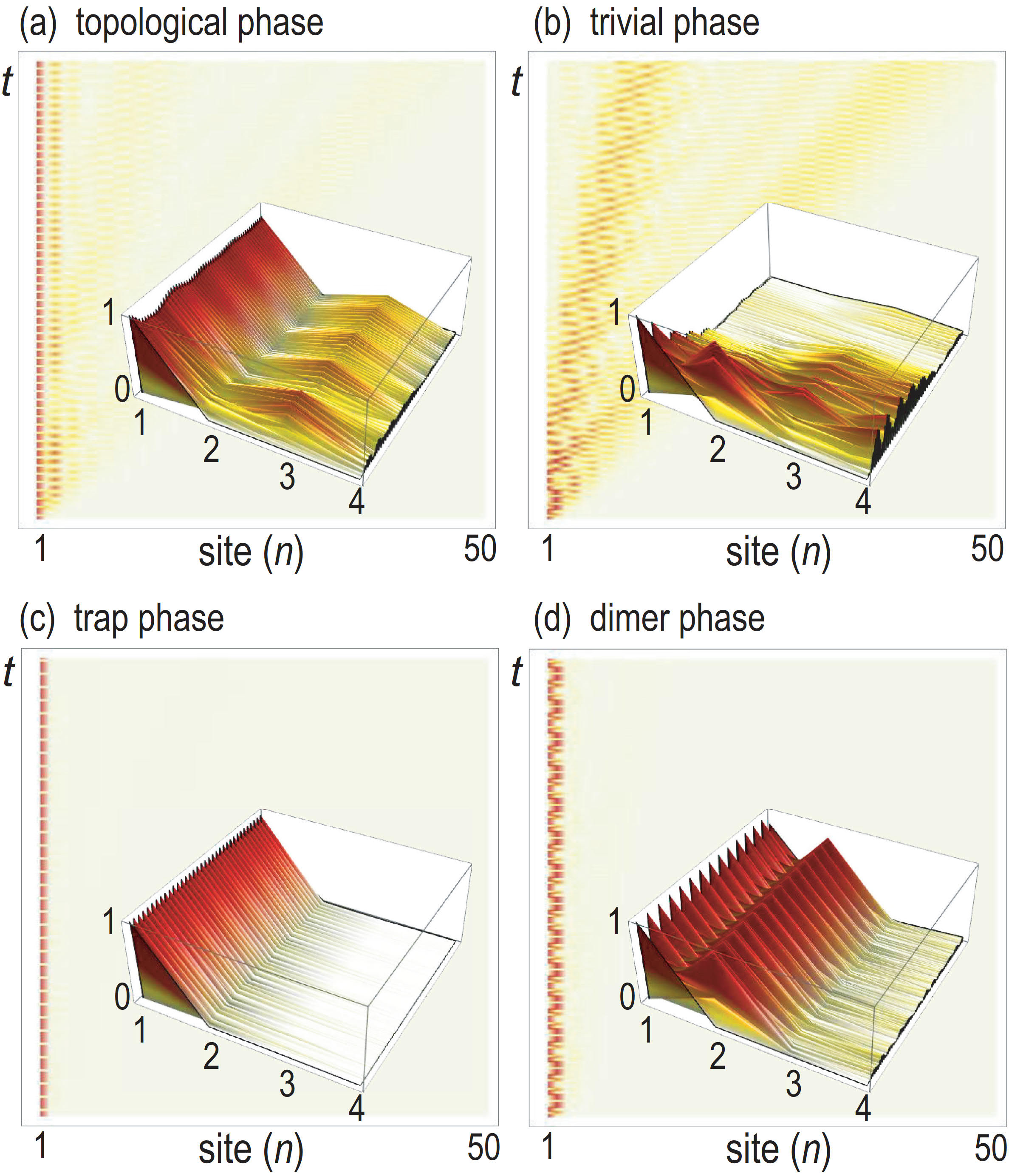
Figure 2: Time evolution of $\Phi_{n}$ in the $n$-th Cooper-pair box. (a) The topological phase with $\lambda=-0.5$ and $\xi=0.25$, where there are simple standing waves at $n=1$ and $n=3$. (b) The trivial phase with $\lambda=0.5$and $\xi=0.25$, where the oscillation propagates along the array. (c) The trap phase with $\lambda=-0.8$ and $\xi=0.8$, where the standing wave is present only at the left-end Cooper-pair box. (d) The dimer phase with $\lambda=0.9$ and $\xi=0.5$, where coupled standing waves are trapped to two Cooper-pair boxes at the left-end. We have used a chain with length $100$. Insets show an enlarged dynamics with length $4$, where the vertical axis is $\Phi_{n}$ in units of $\left(\xi\Phi_{0}/2\right)$. We have set $T=50$.

Dimerized CPB array: To equip the system with a topological structure, we consider a one-dimensional periodic chain, where all capacitances within CPBs are taken equal and the capacitances connecting CPBs are taken to be alternating,

$$C_{A}^{\prime}=C_{2n+1}^{\prime}=C^{\prime}\left(1+\lambda\right),\quad C_{B}^{\prime}=C_{2n}^{\prime}=C^{\prime}\left(1-\lambda\right),$$ (6)

with the dimerization $\left|\lambda\right|\leq 1$. We write down Eq. (4) explicitly as follows,

$$C_{B}^{\prime}\ddot{\Phi}_{2n-2}-\left(C+2C^{\prime}\right) \ddot{\Phi}_{2n-1}+C_{A}^{\prime}\ddot{\Phi}_{2n}$$

$$=I_{\text{c}}\sin 2\pi(\Phi_{2n-1}/\Phi_{0}),$$ (7)

$$C_{A}^{\prime}\ddot{\Phi}_{2n-1}-\left(C+2C^{\prime}\right) \ddot{\Phi}_{2n}+C_{B}^{\prime}\ddot{\Phi}_{2n+1}$$

$$=I_{\text{c}}\sin 2\pi(\Phi_{2n}/\Phi_{0}).$$ (8)

Our task is to solve these equations. The flux $\Phi_{n}$ propagates as shown in Fig.2. Accordingly, the charge $Q_{n}$ also propagates along the array with the use of the solution $\Phi_{n}$ according to the formula (5).

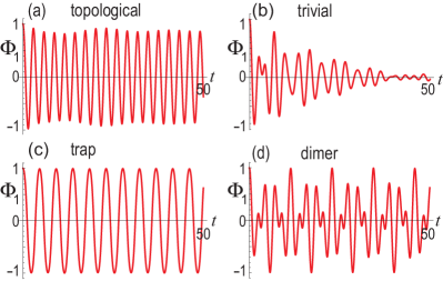
Figure 3: Time evolution of $\Phi_{1}$ in units of $\left(\xi\Phi_{0}/2\right)$. (a) A topological phase with $\lambda=-0.5$ and $\xi=0.25$ (b) a trivial phase with $\lambda=0.5$ and $\xi=0.25$, (c) trap phase with $\lambda=-0.8$ and $\xi=0.8$ and (d) the dimer phase with $\lambda=0.9$ and $\xi=0.5$. We have set and $I_{\text{c}}=10$ and used a chain with the length $100$ and set $T=50$.

Quench dynamics and phase diagram: We investigate the quench dynamics by taking the initial condition such as

$$\Phi_{n}=\frac{1}{2}\xi\Phi_{0}\delta_{n,1},\quad\dot{\Phi}_{n}=0,$$ (9)

with $0\leq\xi\leq 1$. Namely, we give the initial flux with the strength $\frac{1}{2}\xi\Phi_{0}$ only to the left-end CPB. Then, allowing it to move with the zero initial velocity, we study how the motion propagates along the array. We see later that the strength $\xi$ controls the nonlinearity of the system.

We have examined the quench dynamics by taking various values of $\lambda$ and $\xi$. We have found numerically that there are four types of propagations, whose typical structures are given in Fig.2. The time evolution at the edge, $\Phi_{1}\left(t\right)$, is shown in Fig.3 for these four types of propagations.

In Fig.2(a), there are standing waves mainly at the left-end CPB and weakly at a few adjacent odd-number CPBs. Furthermore, there are propagating waves into other CPBs. In Fig.2(b), there are only propagating waves into other CPBs. In Fig.2(c), the standing wave is trapped strictly at the left-end CPB. In Fig.2(d), the coupled standing waves are trapped to double CPBs at the left-end.

We next search for the phase diagram in the $\lambda$-$\xi$ plane. We define the phase indicator by the saturated amplitude as

$$\Psi\equiv\max_{T_{1}<t<T_{2}}\frac{\left|\Phi_{1}\left(t\right)\right|}{\xi\Phi_{0}/2},$$ (10)

where $T_{1}$ and $T_{2}$ are taken much larger than the period and $T_{2}-T_{1}$ is of the order of the period of the modulation.

First, we show it as a function of $\lambda$ in Fig.4(a). It exhibits a sharp transition at $\lambda=0$, which is finite for $\lambda<0$ and almost zero for $\lambda>0$ in the weak nonlinear regime $\xi\lesssim 1/2$. It must be a phase transition separating the two phases with $\lambda<0$ and $\lambda>0$. We also show $\Psi$ in the $\lambda$-$\xi$ plane in Fig.5. Later we argue that they are the topological and trivial phases. We find that the phase boundary remains as it is for $\xi\lesssim 1/2$.

There are two more phases with the phase transition points identified by gaps in the phase indicator in Fig.4(b). One is present around the upper-left corner of Fig.5(b), which we call the trap phase because the wave is trapped to the left-end CPB by the nonlinear effect as in Fig.2(c). The other is present along the right side, which we call the dimer phase since its origin is the dimer mode as in Fig.2(d). We later ague that the former is well approximated by a single CPB and the latter by double CPBs.

These four phases are distinguishable by the time evolution of propagating modes. There is a stable oscillation although the amplitude is smaller than 1 in the topological phase as shown in Fig.3(a). The amplitude rapidly decreases in the trivial phase as shown in Fig.3(b). The oscillation with the amplitude 1 is observed in the trap phase as shown in Fig.3(c). There is a beating oscillation in the dimer phase as shown in Fig.3(d).

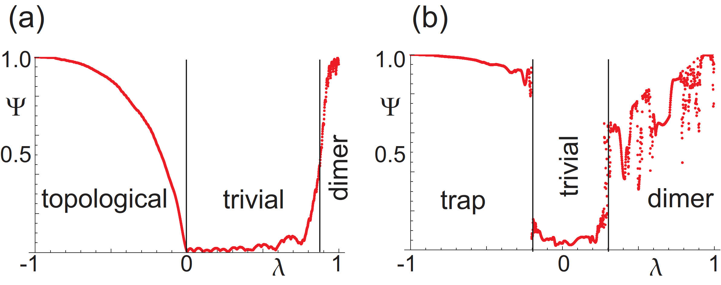
Figure 4: Phase indicator $\Psi$ as a function of dimerization $\lambda$. (a) $\xi=0.25$ and (b) $\xi=0.8$. We have set $I_{\text{c}}=10$ and used a chain with the length $100$. We have set $T_{1}=45$ and $T_{2}=50$.

Topological argument: In order to clarify the topological property of the dynamics, we study the hopping matrix $M_{nm}$ in Eq.(4). We split the hopping matrix between the diagonal and the off-diagonal terms as

$$M_{nm}=\left(C+2C^{\prime}\right)\delta_{nm}-\overline{M}_{nm},$$ (11)

where

$$\overline{M}_{nm} = [C_{A}^{\prime}\delta_{m,n+1}+C_{B}^{\prime}\delta_{n,m+1}]\quad\text{for odd }n,$$

$$\overline{M}_{nm} = [C_{B}^{\prime}\delta_{m,n+1}+C_{A}^{\prime}\delta_{n,m+1}]\quad\text{for even }n.$$ (12)

Here, $\overline{M}_{nm}$ describes the SSH model, which is typical topological model.

In the momentum space, it reads

$$\overline{M}\left(k\right)=\left(\begin{array}[]{cc}0&q\left(k\right)\\ q^{\ast}\left(k\right)&0\end{array}\right)$$ (13)

with $q\left(k\right)=C_{A}^{\prime}+C_{B}^{\prime}e^{-ik}$. The topological number is the Zak phase defined by

$$\Gamma=\frac{1}{2\pi}\int_{0}^{2\pi}A\left(k\right)dk,$$ (14)

where $A\left(k\right)=-i\left\langle\psi(k)\right|\partial_{k}\left|\psi(k)\right\rangle$ is the Berry connection with $\psi(k)$ the eigenfunction of $M_{0}\left(k\right)$. It is well known that the system is topological ($\Gamma=1$) for $C_{B}^{\prime}>C_{A}^{\prime}$ and trivial ($\Gamma=0$) for $C_{B}^{\prime}<C_{A}^{\prime}$ in the SSH model.

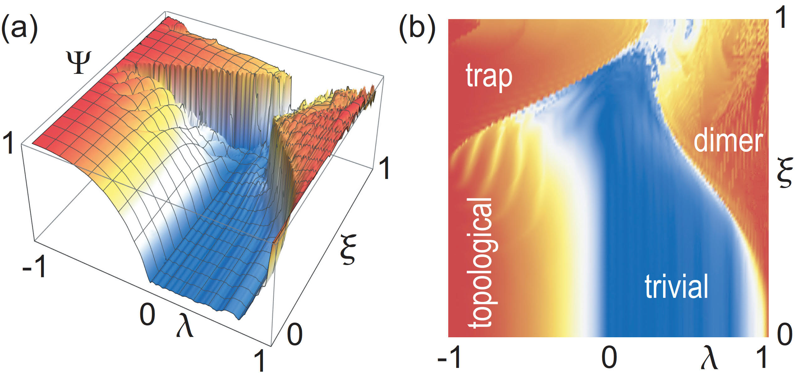
Figure 5: Phase indicator $\Psi$ in the $\lambda$-$\xi$ plane. (a) Bird’s eye’s view and (b) Top view. We have set $I_{\text{c}}=10$ and used a chain with the length $100$. We have set $T_{1}=45$ and $T_{2}=50$.

Linearized theory: Although the hopping matrix $M_{nm}$ has a topological structure, it is not clear how the topological property manifests itself in the CPB array because it is a part of the kinetic term. We now argue that the phase diagram in Fig.5 is just the topological phase diagram.

We have found in Fig.5 that the phase boundary at $\lambda=0$ is almost identical in a wide region for $\xi<1/2$. We construct a linearized theory near $\xi=0$, where the equations of motions read

$$\sum_{m}M_{nm}\ddot{\Phi}_{n}+2\pi I_{\text{c}}\Phi_{n}/\Phi_{0}=0.$$ (15)

We diagonalize the hopping matrix as

$$M_{nm}\Phi_{m}^{\left(p\right)}=E_{p}\Phi_{m}^{\left(p\right)},$$ (16)

where $p$ labels the eigenvalue. In the basis of the eigenfunction, the equations of motion is given by

$$E_{p}\ddot{\Phi}_{m}^{\left(p\right)}=-2\pi I_{\text{c}}\Phi_{m}^{\left(p\right)}/\Phi_{0},$$ (17)

whose solutions are

$$\Phi_{m}^{\left(p\right)}\left(t\right)=\exp\left[\pm i\Omega_{p}t\right]\Phi_{m}^{\left(p\right)}\left(0\right),$$ (18)

with the characteristic frequency $\Omega_{p}\equiv 2\pi I_{\text{c}}/\Phi_{0}E_{p}$. This is also the solution of Eq.(15).

The eigenfunction $\Phi_{m}^{\left(p\right)}$ is that of the SSH model $\overline{M}_{nm}$ as well. In the topological phase of the SSH model, there are zero-energy edge states $\Phi_{m}^{\left(0\right)}$ localized at the edges ($\overline{E}_{0}=0$). They describe also the localized edge states with the energy $E_{0}=C+2C^{\prime}$ in Eq.(16). They remain at the edge after the time evolution. On the other hand, there are no such localized edge states in the trivial phase, and hence, there are no modes remaining at the edge. These phenomena are the clear distinction between the topological and the trivial phases in the present Cooper-box array. We have numerically confirmed that they are valid even in the nonlinear regime.

Topological and trap phases: In Fig.2(a) and (c), the dynamics is induced mainly at the left edge. Time evolution of $\Phi_{1}$ is shown in Fig.3(a) and (c). In order to obtain analytic understanding, we consider the limit $\lambda\rightarrow-1$, where the left-end CPB is detached from the rest since $C_{A}^{\prime}=0$.

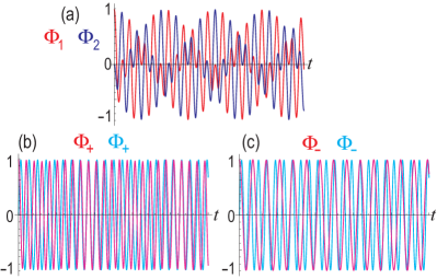
Figure 6: The dynamics of double Cooper-pair boxes. We have set $\xi=0.1$. (a) $\Phi_{1}$ in red and $\Phi_{2}$ in blue. (b) $\Phi_{+}$ and (c) $\Phi_{-}$. (b) and (c) The numerical results are show in magenta and the analytic solutions (25) and (26) are shown in cyan. We have set $\xi=0.25$ and $I_{\text{c}}=10$.

The equation of motion for the left-end CPB in Fig.1(c) is given by

$$\ddot{\Phi}_{1}=-(I_{\text{c}}/C)\sin 2\pi(\Phi_{1}/\Phi_{0}).$$ (19)

The exact solution is given by

$$\Phi_{1}(t)=2\Phi_{0}\sin^{-1}[\alpha\sin\text{am}(\alpha,\omega t+K\left(k\right))],$$ (20)

where am is the Jacobi amplitude function, $K\left(k\right)$ is the Jacobi perfect elliptic integral of the first kind, $\omega\equiv\sqrt{I_{\text{c}}/C}$ and $\alpha$ is determined as $\alpha=\sin[\Phi\left(0\right)/2]$ in terms of the initial condition $\Phi(0)$. The period is given by $T=4\omega^{-1}K\left(k\right)$. This solution well describes the wave function of the topological edge state numerically obtained.

The solution (20) is valid at $\lambda=-1$ irrelevant of the value of $\xi$. Hence, it describes the topological edge state in the topological phase as well as the edge state in the trap phase. Indeed, we have numerically checked that this single CPB wavefunction well describes the edge state for the topological phase and the trap phase in Fig.3(a) and (c). Actually, there is no transition between the topological and trap phases at $\lambda=-1$. However, numerical solutions show that there is a sharp transition between the topological and trap phases for $\lambda>-1$. The topological phase is smoothly connected with that of the linear theory. However, the trap phase is not connected with any phase in the linear theory. Especially, we cannot assign a topological number for the trap phase because it is an isolated oscillation mode.

Dimer phase: In Fig.2(d), the dynamics is induced solely at the left two edges. Time evolution of $\Phi_{1}$ is shown in Fig.3(d). In order to obtain analytic understanding, we consider the limit $\lambda\rightarrow 1$, where the left-end double CPBs are detached from the rest since $C_{B}^{\prime}=0$.

We analyze the dynamics of a pair of CPBs connected via a capacitor[50] as shown in Fig.1(b). The equations of motions read

$$\left(C+C^{\prime}\right)\ddot{\Phi}_{1}-C^{\prime}\ddot{\Phi}_{2} =-I_{\text{c}}\sin 2\pi(\Phi_{1}/\Phi_{0}),$$ (21)

$$\left(C+C^{\prime}\right)\ddot{\Phi}_{2}-C^{\prime}\ddot{\Phi}_{1} =-I_{\text{c}}\sin 2\pi(\Phi_{2}/\Phi_{0}).$$ (22)

We numerical solve these equations with the initial condition (9), whose result is shown in Fig.6(a). The beating behavior is observed. We plot $\Phi_{+}\equiv\Phi_{1}+\Phi_{2}$ and $\Phi_{-}\equiv\Phi_{1}-\Phi_{2}$ in Fig.6(b) and (c). The equations of motion reads

$$\ddot{\Phi}_{+} =-(I_{\text{c}}/C)\sin\pi(\Phi_{+}/\Phi_{0})\cos\pi(\Phi_{-}/\Phi_{0}),$$ (23)

$$\ddot{\Phi}_{-} =-(I_{\text{c}}/\left(C+2C^{\prime}\right))\cos\pi(\Phi_{+}/\Phi_{0})\sin\pi(\Phi_{-}/\Phi_{0}),$$ (24)

whose approximate solutions are

$$\Phi_{+}\left(t\right) =2\Phi_{0}\sin^{-1}[\alpha\sin\text{am}(\alpha,\omega_{+}t+K\left(k\right))],$$ (25)

$$\Phi_{-}\left(t\right) =2\Phi_{0}\sin^{-1}[\alpha\sin\text{am}(\alpha,\omega_{-}t+K\left(k\right))],$$ (26)

with $\omega_{+}\equiv\sqrt{I_{\text{c}}/C}$, $\omega_{-}\equiv\sqrt{I_{\text{c}}/(C+2C^{\prime})}$ and $\alpha\equiv\sin[\Phi\left(0\right)/2]$. The period of $\Phi_{+}\left(t\right)$ is $T=4K\left(k\right)/\omega_{+}$ and that of $\Phi_{-}\left(t\right)$ is $T=4K\left(k\right)/\omega_{-}$. In numerical simulations, there are fluctuation of the period although the overall period is identical to the analytic solution.

We have found a dynamical topological phase transition in a CPB array, which is absent in static system. It is highly contrasted to standard models, where the topological phase is present in static system. It is possible to realize the present system by using existing superconducting qubit systems.

The author is very much grateful to N. Nagaosa for helpful discussions on the subject. This work is supported by CREST, JST (JPMJCR20T2).

References

- [1] M. Z. Hasan and C. L. Kane, Rev. Mod. Phys. 82, 3045 (2010).
- [2] X.-L. Qi and S.-C. Zhang, Rev. Mod. Phys. 83, 1057 (2011).
- [3] A. B. Khanikaev, S. H. Mousavi, W.-K. Tse, M. Kargarian, A. H. MacDonald, G. Shvets, Nature Materials 12, 233 (2013).
- [4] M. Hafezi, E. Demler, M. Lukin, J. Taylor, Nature Physics 7, 907 (2011).
- [5] M. Hafezi, S. Mittal, J. Fan, A. Migdall, J. Taylor, Nature Photonics 7, 1001 (2013).
- [6] L.H. Wu and X. Hu, Phys. Rev. Lett. 114, 223901 (2015).
- [7] L. Lu. J. D. Joannopoulos and M. Soljacic, Nature Photonics 8, 821 (2014).
- [8] T. Ozawa, H. M. Price, A. Amo, N. Goldman, M. Hafezi, L. Lu, M. C. Rechtsman, D. Schuster, J. Simon, O. Zilberberg and L. Carusotto, Rev. Mod. Phys. 91, 015006 (2019).
- [9] E. Prodan and C. Prodan, Phys. Rev. Lett. 103, 248101 (2009).
- [10] Z. Yang, F. Gao, X. Shi, X. Lin, Z. Gao, Y. Chong and B. Zhang, Phys. Rev. Lett. 114, 114301 (2015).
- [11] P. Wang, L. Lu and K. Bertoldi, Phys. Rev. Lett. 115, 104302 (2015).
- [12] M. Xiao, G. Ma, Z. Yang, P. Sheng, Z. Q. Zhang and C. T. Chan, Nat. Phys. 11, 240 (2015).
- [13] C. He, X. Ni, H. Ge, X.-C. Sun,Y.-B. Chen1 M.-H. Lu, X.-P. Liu, L. Feng and Y.-F. Chen, Nature Physics 12, 1124 (2016).
- [14] C. L. Kane and T. C. Lubensky, Nature Phys. 10, 39 (2014).
- [15] B. Gin-ge Chen, N. Upadhyaya and V. Vitelli, PNAS 111, 13004 (2014).
- [16] L. M. Nash, D. Kleckner, A. Read, V. Vitelli, A. M. Turner and W. T. M. Irvine, PNAS 112, 14495 (2015).
- [17] J. Paulose, A. S. Meeussen and V. Vitelli, PNAS 112, 7639 (2015).
- [18] R. Susstrunk, S. D. Huber, Science 349, 47 (2015).
- [19] R. Susstrunk and S. D. Huber, Proc. Natl. Acad. Sci. USA 113, E4767 (2016).
- [20] S. D. Huber, Nature Physics 12, 621 (2016).
- [21] A. S. Meeussen, J. Paulose and V. Vitelli, Phys. Rev. X 6, 041029 (2016).
- [22] S. Imhof, C. Berger, F. Bayer, J. Brehm, L. Molenkamp, T. Kiessling, F. Schindler, C. H. Lee, M. Greiter, T. Neupert, R. Thomale, Nat. Phys. 14, 925 (2018).
- [23] C. H. Lee , S. Imhof, C. Berger, F. Bayer, J. Brehm, L. W. Molenkamp, T. Kiessling and R. Thomale, Communications Physics, 1, 39 (2018).
- [24] T. Helbig, T. Hofmann, C. H. Lee, R. Thomale, S. Imhof, L. W. Molenkamp and T. Kiessling, Phys. Rev. B 99, 161114 (2019).
- [25] Y. Lu, N. Jia, L. Su, C. Owens, G. Juzeliunas, D. I. Schuster and J. Simon, Phys. Rev. B 99, 020302 (2019).
- [26] Y. Li, Y. Sun, W. Zhu, Z. Guo, J. Jiang, T. Kariyado, H. Chen and X. Hu, Nat. Com. 9, 4598 (2018).
- [27] M. Ezawa, Phys. Rev. B 98, 201402(R) (2018).
- [28] D. Leykam and Y. D. Chong, Phys. Rev. Lett. 117, 143901 (2016).
- [29] X. Zhou, Y. Wang, D. Leykam and Y. D. Chong, New J. Phys. 19, 095002 (2017).
- [30] L. J. Maczewsky, M. Heinrich, M. Kremer, S. K. Ivanov, M. Ehrhardt, F. Martinez, Y. V. Kartashov, V. V. Konotop, L. Torner, D. Bauer, A. Szameit, Science 370, 701 (2010).
- [31] Y. Hadad, Alexander B. Khanikaev and Andrea Alu Phys. Rev. B 93, 155112 (2016)
- [32] D. Smirnova, D. Leykam, Y. Chong and Y. Kivshar, Applied Physics Reviews 7, 021306 (2020).
- [33] T. Tuloup, R. W. Bomantara, C. H. Lee and J. Gong, Phys. Rev. B 102, 115411 (2020).
- [34] S. Kruk, A. Poddubny, D. Smirnova, L. Wang, A. Slobozhanyuk, A. Shorokhov, I. Kravchenko, B. Luther-Davies and Y. Kivshar, Nature Nanotechnology 14, 126 (2019).
- [35] M. Ezawa, Phys. Rev. B 104, 235420 (2021).
- [36] M. S. Kirsch, Y. Zhang, M. Kremer, L. J. Maczewsky, S. K. Ivanov, Y. V. Kartashov, L. Torner, D. Bauer, A. Szameit and M. Heinrich, Nature Physics 17, 995 (2021).
- [37] D. D. J. M. Snee, Y.-P. Ma, Extreme Mechanics Letters 100487 (2019).
- [38] P.-W. Lo, K. Roychowdhury, B. G.-g. Chen, C. D. Santangelo, C.-M. Jian, M. J. Lawler, Phys. Rev. Lett. 127, 076802 (2021).
- [39] M. Ezawa, J. Phys. Soc. Jpn. 90, 114605 (2021).
- [40] Y. Hadad, J. C. Soric, A. B. Khanikaev, and A. Alù, Nature Electronics 1, 178 (2018).
- [41] K. Sone, Y. Ashida, T. Sagawa, Phys. Rev. Research 4, 023211 (2022).
- [42] M. Ezawa, J. Phys. Soc. Jpn. 91, 024703 (2022).
- [43] T. Kotwal, F. Moseley, A. Stegmaier, S. Imhof, H. Brand, T. Kieling, R. Thomale, H. Ronellenfitsch and J. Dunkel, PNAS 118 (32) e2106411118 (2021)
- [44] Y. Nakamura; Yu. A. Pashkin; J. S. Tsai, Nature 398, 786 (1999).
- [45] F. Arute, et.al., Nature, 574, 505 (2019)
- [46] J. Koch, T. M. Yu, J. Gambetta, A. A. Houck, D. I. Schuster, J. Majer, A. Blais, M. H. Devoret, S. M. Girvin and R. J. Schoelkopf, Phys. Rev. A 76, 042319 (2007)
- [47] J. A. Schreier, A. A. Houck, Jens Koch, D. I. Schuster, B. R. Johnson, J. M. Chow, J. M. Gambetta, J. Majer, L. Frunzio, M. H. Devoret, S. M. Girvin, and R. J. Schoelkopf, Phys. Rev. B 77, 180502(R) (2008)
- [48] V. Bouchiat, D. Vion, P. Joyez, D. Esteve and M. H. Devoret, Phys. Scr. 165 (1998)
- [49] Yuriy Makhlin, Gerd Schoen, and Alexander Shnirman, Rev. Mod. Phys. 73, 357 (2001)
- [50] P. Krantz, M. Kjaergaard, F. Yan, T. P. Orlando, S. Gustavsson and W. D. Oliver, Applied Physics Reviews 6, 021318 (2019)