On stochastic control under Poisson observations: optimality of a barrier strategy in a general Lévy model

Abstract.

We study a version of the stochastic control problem of minimizing the sum of running and controlling costs, where control opportunities are restricted to independent Poisson arrival times. Under a general setting driven by a general Lévy process, we show the optimality of a periodic barrier strategy, which moves the process upward to the barrier whenever it is observed to be below it. The convergence of the optimal solutions to those in the continuous-observation case is also shown.

AMS 2020 Subject Classifications: 60G51, 93E20, 90B05
Keywords: stochastic control, inventory models, periodic observations, mathematical finance, Lévy processes

1. Introduction

Stochastic control aims to obtain an optimal dynamic strategy in cases of uncertainty. In its typical formulation, the problem reduces to obtaining an adapted control process that maximizes/minimizes the expected total reward/cost, which depends on the paths of the controlling and controlled processes. The continuous-time stochastic control research, active in various fields such as financial/actuarial mathematics and research on inventory models, has been developed along with stochastic analysis and differential equations theory. In contrast with its discrete-time counterpart, for which numerical approaches are typically required, various analytical approaches, such as Itô calculus and first passage analysis, are available in continuous-time models to obtain explicit results.

Poissonian observation models have been developed to explore the interface between continuous-time and discrete-time models (see [1, 2, 11, 18, 21, 22, 26, 27]). Instead of allowing the decision maker to observe the state process continuously and control it at all times, these opportunities are given only at independent Poisson arrival times. With the selection of exponential interarrival times, the problem often continues to be analytically tractable, thanks mainly to the memoryless property of the exponential random variables. Although this assumption of Poisson arrivals is indeed restrictive in real applications, it provides a more flexible approach for approximating the discrete-time counterpart (with deterministic interarrivals) than the classical continuous-time model. As confirmed numerically in studies such as [17], approximation via Poisson arrivals (as a special case of Erlanization [9, 16]) often achieves accurate approximation of the discrete-time model in stochastic control problems.

This paper studies the classical stochastic control problem, described as follows. Given a stochastic process $X=\{X_{t}:t\geq 0\}$, the objective is to choose a strategy $\pi=\{R_{t}^{\pi}:t\geq 0\}$ to minimize the total expected values of the running cost $\int_{0}^{\infty}e^{-qt}f(U_{t}^{\pi}){\rm d}t$ and the controlling cost $\int_{[0,\infty)}e^{-qt}{\rm d}R_{t}^{\pi}$, where $U^{\pi}:=X+R^{\pi}$ is the controlled process when $\pi$ is applied. Various problems can be modeled in this framework by appropriately choosing the process $X$. See [3, 4, 5] for inventory models and [8, 13, 19] for financial applications.

This problem has been studied in several papers when $X$ is a spectrally negative Lévy process (i.e., a Lévy process with only negative jumps). Under the assumption that the running cost function is convex, the barrier strategy, with the lower barrier $b^{*}$ selected to be a unique root of

(1.1) $$\mathbb{E}_{b}\left[\int_{0}^{\infty}e^{-qt}f^{\prime}_{+}(U^{b}_{t}){\rm d}t\right]+C=0,$$

is optimal. Here, $U^{b}$ is the reflected process starting at $b$, with a lower barrier $b$, which is also called a draw-up or an excursion in the literature. Interestingly, this optimality result continuous to hold under non-standard formulations. In a version where $R^{\pi}$ is restricted to being absolutely continuous with respect to the Lebesgue measure with a given density bound [12], the same optimality result holds, with $U^{b}$ being the so-called refracted processes [15, 24]. The Poissonian observation version we consider in this paper has been solved by [23] for the spectrally negative case. In this case, $U^{b}$ is a version of the reflected process that is pushed to $b$ whenever it is observed to be below it. By selecting the barrier using (1.1), this version of the barrier strategy, which we call the periodic barrier strategy, has been shown to be optimal.

The results described above all rely on the so-called scale function (see [6, 14]), which makes sense only for spectrally one-sided Lévy processes. The expected cost under barrier strategies can be written concisely via the scale function, with which the smoothness of the value function and its optimality can be verified in a straightforward way. However, the spectrally negative assumption is often unrealistic in real applications. For example, financial asset prices are empirically known to have both positive and negative jumps (see [10]); also, water storage levels of dams experience both positive and negative jumps, due to rainfall and surges in consumption.

Although the existing results for a general Lévy process in stochastic control are significantly limited in comparison with diffusion and spectrally one-sided Lévy models, the problem described above has recently been solved for a general Lévy process in the continuous-observation setting. Noba and Yamazaki [20] has shown that the classical barrier strategy described in (1.1) continues to be optimal even in the presence of positive jumps. It is thus a natural conjecture that the form of optimal strategy is invariant to the existence of upward jumps, and the same optimality result holds more generally, even under non-standard formulations.

The objective of this paper is to verify this conjecture. We solve the Poissonian observation case for a general Lévy process $X$ with both positive and negative jumps. This generalizes the results of [23] and [20] simultaneously and provides a unified way of expressing the optimal strategy. The difficulty is that we need a new approach, one which is capable of handling a general Lévy process of finite and infinite activity/variations – but without relying on the scale function method. Despite the obvious difficulties regarding Poissonian observation models, for which much less analytical results are available in comparison to the classical case, we provide a more concise proof than those given in [20]. By focusing on the Poissonian observation setting, the variational inequality is more easily verified, and the value function tends to be smoother. Furthermore, we demonstrate that the optimal solutions in the Poissonian setting converge to those in the continuous-observation setting. These results potentially provide a new approach to the classical case, by way of the techniques developed in this paper for Poisson observation models.

Thanks to the explicit and concise expression of the optimal barrier $b^{*}$ as a solution to (1.1), the optimal barrier as well as the value function can be computed generally via a standard Monte Carlo simulation. We demonstrate that this can be done efficiently through a sequence of numerical examples and also confirm the convergence as the observation rate increases to infinity.

The rest of the paper is organized as follows. In Section 2, we formally define the problem under consideration. In Section 3, we define periodic barrier strategies and obtain their key properties. Then, in Section 4, we select the barrier and demonstrate the optimality. In Section 5, we show the convergence as the rate of observation goes to infinity to the ones in the classical setting. We conclude the paper with numerical results in Section 6.

2. Problem

Let $X=\{X_{t}:t\geq 0\}$ be a (one-dimensional) Lévy process defined on a probability space $(\Omega,\mathcal{F},\mathbb{P})$. For $x\in\mathbb{R}$, we denote by $\mathbb{P}_{x}$ the law of $X$ when its initial value is $x$, and write $\mathbb{P}=\mathbb{P}_{0}$ for the case $x=0$. Let $\Psi$ be the characteristic exponent of $X$; i.e. $e^{-t\Psi(\lambda)}=\mathbb{E}\left[e^{i\lambda X_{t}}\right]$, $\lambda\in\mathbb{R}$ and $t\geq 0$. It is known to admit the form

(2.1) $$\Psi(\lambda):=-i\gamma\lambda+\frac{1}{2}\sigma^{2}\lambda^{2}+\int_{\mathbb{R}\backslash\{0\}}(1-e^{i\lambda z}+i\lambda z1_{\{|z|<1\}})\Pi({\rm d}z),\qquad\lambda\in\mathbb{R},$$

for some $\gamma\in\mathbb{R}$, $\sigma\geq 0$, and a Lévy measure $\Pi$ on $\mathbb{R}\backslash\{0\}$ satisfying $\int_{\mathbb{R}\backslash\{0\}}(1\land z^{2})\Pi({\rm d}z)<\infty$.

We consider a version of the stochastic control problem defined as follows. The set of control opportunities

$$\mathcal{T}_{\eta}:=\{T(k):k\in\mathbb{N}\}$$

are given by the arrival times of a Poisson process $N^{\eta}=\{N^{\eta}_{t}:t\geq 0\}$ with intensity $\eta>0$ which is independent of $X$. In other words, the interarrival times $\{T(k)-T(k-1):k\in\mathbb{N}\}$ are an i.i.d. sequence of exponential random variables with intensity $\eta$ where we let $T(0)=0$ for notational convenience. Let $\mathbb{F}:=\{{\mathcal{F}_{t}}:t\geq 0\}$ be the natural filtration generated by $(X,N^{\eta})$. A strategy, representing the cumulative amount of controlling, $\pi=\{R^{\pi}_{t}:t\geq 0\}$ is a process of the form

(2.2) $$R^{\pi}_{t}={\int_{[0,t]}\nu^{\pi}_{s}{\rm d}N^{\eta}_{s}}\qquad t\geq 0,$$

for some càglàd and non-negative $\mathbb{F}$-adapted process $\nu^{\pi}=\{\nu^{\pi}_{t}:t\geq 0\}$. The corresponding controlled process becomes

(2.3) $$U^{\pi}_{t}=X_{t}+R^{\pi}_{t},\quad t\geq 0.$$

For a given discount factor $q>0$ and initial value $x\in\mathbb{R}$, the objective is to minimize

$$v_{\pi}(x):=\mathbb{E}_{x}\left[\int_{0}^{\infty}e^{-qt}f(U^{\pi}_{t}){\rm d}t+C\int_{0}^{\infty}e^{-qt}{\rm d}R^{\pi}_{t}\right],$$

which is the sum of running cost for a given measurable function $f:\mathbb{R}\to\mathbb{R}$ and a controlling cost/reward for a unit cost/reward $C\in\mathbb{R}$ (cost if it is positive and reward if negative). Let $\mathcal{A}$ be the set of all admissible strategies satisfying the constraints described above as well as the integrability condition:

(2.4) $$\mathbb{E}_{x}\left[\int_{0}^{\infty}e^{-qt}{|f(U^{\pi}_{t})|}{\rm d}t+\int_{0}^{\infty}e^{-qt}{\rm d}R^{\pi}_{t}\right]<\infty.$$

The aim of the problem is to obtain the (optimal) value function

(2.5) $$v(x):=\inf_{\pi\in\mathcal{A}}v_{\pi}(x),\quad x\in\mathbb{R},$$

and the optimal strategy $\pi^{\ast}$ such that $v_{\pi^{*}}(x)=v(x)$ (if such a strategy exists).

For the running cost function $f$, the unit cost/reward $C$ and the Lévy process $X$, we impose the same conditions as those assumed in [20]; similar conditions are commonly assumed in the literature (see [4, 5, 12, 25]).

Assumption 2.1 (Assumption on $f$ and $C$).

1. The function $f$ is convex.

2. There exist $k_{1}$, $k_{2}$ and $N\in\mathbb{N}$ such that $|f(x)|\leq k_{1}+k_{2}{|x|^{N}}$ for all $x\in\mathbb{R}$.

3. We have $f^{\prime}_{+}(-\infty)<-Cq<f^{\prime}_{+}(\infty)$ where $f^{\prime}_{+}(-\infty):=\lim_{x\to-\infty}f^{\prime}_{+}(x)\in[-\infty,\infty)$ and $f^{\prime}_{+}(\infty):=\lim_{x\to\infty}f^{\prime}_{+}(x)\in(-\infty,\infty]$.

Note that the right- and left-hand derivatives $f^{\prime}_{+}(x)$ and $f^{\prime}_{-}(x)$, respectively, for all $x\in\mathbb{R}$ as well as their limits are well-defined by Assumption 2.1(1). Assumption 2.1(3) is necessary to avoid the optimality of a trivial strategy; see [20, Remark 1].

Assumption 2.2 (Assumption on $X$).

1. $X$ is not a driftless compound Poisson process.

2. For some $\bar{\theta}>0$, $\int_{\mathbb{R}\backslash(-1,1)}e^{\bar{\theta}|z|}\Pi({\rm d}z)<\infty$.

Remark 2.1.

By Assumption 2.2(1) and [6, Proposition I.15], the potential measure of $X$ has no masses. This also shows $\mathbb{P}_{x}(X_{T(1)}=b)={\eta}\mathbb{E}_{x}\left[\int_{0}^{\infty}e^{-{\eta}t}1_{\{X_{t}=b\}}{\rm d}t\right]=0$ for all $x,b\in\mathbb{R}$.

Assumption 2.2(2) together with [14, Theorem 3.6] guarantees the finiteness of $\mathbb{E}[\exp(\bar{\theta}{|X_{1}|})]$ and also that of $\mathbb{E}\left[|X_{1}|\right]$ (since $\exp(x)\geq x$ for $x\geq 0$).

Remark 2.2.

From Assumptions 2.1(2) and 2.2(2) and by the proof of [25, Lemma 11], the expectation $\mathbb{E}_{x}\left[\int_{0}^{\infty}e^{-qt}|f(X_{t})|{\rm d}t\right]$ is finite and it is at most of polynomial growth as $x\uparrow\infty$ and $x\downarrow-\infty$.

3. Periodic barrier strategies

Our objective is to show the optimality of a periodic barrier strategy $\pi^{b}$ for a suitable selection of the barrier $b\in\mathbb{R}$ in the considered stochastic control problem.

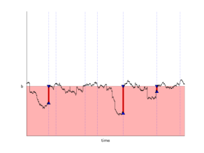
Figure 1. Sample path of $U^{b}$. Control opportunities $\mathcal{T}_{\eta}$ are shown by dotted vertical lines. The control times $\{T_{b}^{(n)}:n\in\mathbb{N}\}$ and control sizes $\Delta R^{b}$ are indicated by the vertical red lines.

Fix $b\in\mathbb{R}$. A periodic barrier strategy $\pi^{b}$ pushes upward the process to $b$ whenever it is observed to be below $b$ (see Figure 1). The epochs of controlling $\{T_{b}^{(n)}:n\in\mathbb{N}\}\subset{\mathcal{T}_{\eta}}$ are given by a sequence of $\mathbb{F}$-stopping times, recursively defined as follows: with $T_{b}^{(0)}:=0$,

(3.1) $$\begin{aligned} T_{b}^{(n)}&=\inf\{t\in\mathcal{T}_{\eta}:t>T_{b}^{(n-1)},\tilde{X}_{t}^{(n-1),b}<b\},\quad n\geq 1,\end{aligned}$$

where

$$\tilde{X}_{t}^{(m),b}:=\begin{cases}X_{t},&m=0,\\ b+(X_{t}-X_{T_{b}^{(m)}}),&m\geq 1,\end{cases}$$

is a parallel shift of $X$ so that it starts from $b$ at $T_{b}^{(m)}$ when $m\geq 1$. The strategy $\pi^{b}$ modifies $X$ by adding at $T_{b}^{(n)}$ the shortage $b-\tilde{X}_{T_{b}^{(n)}}^{(n-1),b}$ so that the path of the controlled process is the concatenation of $(\tilde{X}^{(m),b})_{m\geq 1}$. The corresponding control and controlled processes can be written, respectively,

(3.2) $$R_{t}^{b} :=R_{t}^{\pi^{b}}=\sum_{n=1}^{\infty}(b-\tilde{X}_{T_{b}^{(n)}}^{(n-1),b})1_{\{T_{b}^{(n)}\leq t\}},$$

(3.3) $$U^{b}_{t} :=U^{\pi^{b}}_{t}=X_{t}+R^{b}_{t}=\sum_{n=1}^{\infty}\tilde{X}_{t}^{(n-1),b}1_{\{t\in[T^{(n-1)}_{b},T^{(n)}_{b})\}}.$$

Note that $X$ and $N^{\eta}$ do not jump at the same time.

Alternatively, in terms of the cáglád $\mathbb{F}$-adapted process $\nu^{b}=\{\nu^{b}_{t}:t\geq 0\}$ with

(3.4) $$\nu^{b}_{t}=\begin{cases}\left(b-X_{t-}\right)^{+},\qquad&\qquad t\in[0,T^{(1)}_{b}],\\ {\left(X_{T_{b}^{(n-1)}}-X_{t-}\right)^{+},}\qquad&t\in(T^{(n-1)}_{b},T^{(n)}_{b}]\text{ with }n\geq 2,\end{cases}$$

where $x^{+}:=x\vee 0$ and it is understood that $X_{0-}=X_{0}$, it can be also written

(3.5) $$R^{b}_{t}={\int_{[0,t]}}\nu^{b}_{s}{\rm d}N^{\eta}_{s},\qquad t\geq 0.$$

Remark 3.1.

In terms of the minimum of $X$ observed until time $t$, we can also write

$$R_{t}^{b}=\max_{1\leq k\leq N_{t}^{\eta}}(b-X_{T(k)})^{+},\quad t\geq 0,$$

and $T^{(n)}_{b}$ as the $n$-th jump time of $R^{b}$. This expression will be used to show the convergence to the classical case in Section 5.

For the rest of the paper, we let the expected total cost under the periodic barrier strategy $\pi^{b}$ be written

(3.6) $$v_{b}(x):=v_{\pi^{b}}(x),\quad x\in\mathbb{R}.$$

We now show the admissibility of periodic barrier strategies along with related results. The proof of the following lemma is deferred to Appendix A.1.

Lemma 3.1.

For $x,b\in\mathbb{R}$, (i) $\mathbb{E}_{x}\left[\int_{0}^{\infty}e^{-qt}|f(U^{b}_{t})|{\rm d}t\right]<\infty$ and (ii) $\mathbb{E}_{x}\left[\int_{0}^{\infty}e^{-qt}{\rm d}R^{b}_{t}\right]<\infty$, (iii) $v_{b}$ is at most of polynomial growth.

As a corollary of the above, we also have the following. Thanks to Assumption 2.1(1), this can be shown exactly in the same way as the proof of [20, Lemma 4] and thus we omit the proof.

Corollary 3.1.

For $x,b\in\mathbb{R}$, we have $\mathbb{E}_{x}\left[\int_{0}^{\infty}e^{-qt}\left|f^{\prime}_{+}(U^{b}_{t})\right|{\rm d}t\right]<\infty$.

Lemma 3.1 together with (3.5) shows the following.

Proposition 3.1.

For $b\in\mathbb{R}$, the strategy $\pi^{b}$ is admissible.

Let $T_{b}:=T_{b}^{(1)}$ be the first control time under the policy $\pi^{b}$. We conclude this section with the expression of the slope of $v_{b}$ written in terms of $T_{b}$ and the uncontrolled Lévy process $X$.

Proposition 3.2.

For $b\in\mathbb{R}$, the function $v_{b}$ is continuously differentiable with its derivative

(3.7) $$v_{b}^{\prime}(x)=\mathbb{E}_{x}\left[\int_{0}^{T_{b}}e^{-qt}f^{\prime}_{+}(X_{t}){\rm d}t\right]-C\mathbb{E}_{x}\left[e^{-qT_{b}}\right],\quad x\in\mathbb{R}.$$

The proof of Proposition 3.2 requires the following continuity result of $T_{b}$; its proof is deferred to Appendix A.2.

Lemma 3.2.

For fixd $b\in\mathbb{R}$, we have $\lim_{b^{\prime}\to b}T_{b^{\prime}}=T_{b}$ on $\{T_{b}<\infty\}$, almost surely.

Proof of Proposition 3.2.

By Lemma 3.1, we can decompose the expected costs as follows:

(3.8) $$v_{b}(x)=v_{b}^{(1)}(x)+Cv_{b}^{(2)}(x),\quad x\in\mathbb{R},$$

where we write

(3.9) $$v_{b}^{(1)}(x):=\mathbb{E}_{x}\left[\int_{0}^{\infty}e^{-qt}f(U^{b}_{t}){\rm d}t\right],\quad v_{b}^{(2)}(x):=\mathbb{E}_{x}\left[\int_{0}^{\infty}e^{-qt}{\rm d}R^{b}_{t}\right].$$

For $y\in\mathbb{R}$, we write $X^{[y]}_{t}:=X_{t}+y$, $t\geq 0$, and write $U^{[y],b}$, $R^{[y],b}_{t}$, $T^{[y]}_{b}$ be those corresponding to this shifted process.

(i) Fix $b\in\mathbb{R}$ and $\varepsilon>0$. We show that $t\mapsto U^{[\varepsilon],b}_{t}-U^{b}_{t}=\varepsilon+R^{[\varepsilon],b}_{t}-R^{b}_{t}$ is nonincreasing and always lies on $[0,\varepsilon]$. Because this difference is a step function in $t$ with jump times contained in the set $\mathcal{T}_{\eta}$, it suffices to show

$$\zeta(k):=U^{[\varepsilon],b}_{T(k)}-U^{b}_{T(k)}=\varepsilon+R^{[\varepsilon],b}_{T(k)}-R^{b}_{T(k)},\quad k\geq 0,$$

is nonincreasing in $k$ and takes values only on $[0,\varepsilon]$. We show this claim by induction.

First it holds trivially when $k=0$ with $\zeta(0)={\varepsilon}\in[0,\varepsilon]$.

Now, suppose it holds that $\zeta(k)\in[0,\varepsilon]$ for some $k\geq 0$. With the set of indices of controlling:

$$A^{[\delta]}:=\{k\geq 1:\Delta R_{T(k)}^{[\delta],b}>0\}=\{k\geq 1:U^{[\delta],b}_{T(k-1)}+(X_{T(k)}-X_{T(k-1)})<b\},\quad\delta=0,\varepsilon,$$

we have

(3.10) $$\{k+1\in A^{[\varepsilon]}\}=\{U^{b}_{T(k)}+\zeta(k)+(X_{T(k+1)}-X_{T(k)})<b\}\\ \subset\{U^{b}_{T(k)}+(X_{T(k+1)}-X_{T(k)})<b\}=\{k+1\in A^{[0]}\}.$$

(A) Suppose $k+1\in A^{[\varepsilon]}$ so that $U^{[\varepsilon],b}_{T(k+1)}=b$. By (3.10), this also implies $k+1\in A^{[0]}$ or equivalently $U^{b}_{T(k+1)}=b$. Hence, $\zeta(k+1)=0$.

(B) Suppose $k+1\notin A^{[\varepsilon]}$ so that

(3.11) $$U^{[\varepsilon],b}_{T(k)}+(X_{T(k+1)}-X_{T(k)})\geq b.$$

(a) Suppose $k+1\notin A^{[0]}$, then because $\Delta R^{[\varepsilon],b}_{T(k+1)}=\Delta R^{b}_{T(k+1)}=0$, we have $\zeta(k+1)=\zeta(k)\in[0,\varepsilon]$.

(b) Suppose $k+1\in A^{[0]}$. Then, clearly $\zeta(k+1)=\zeta(k)-\Delta R^{b}_{T(k+1)}<\zeta(k)$. In addition, by (3.11),

$$\zeta(k+1)=(U^{[\varepsilon],b}_{T(k)}+(X_{T(k+1)}-X_{T(k)}))-b\geq 0.$$

In sum, in all cases we have $\zeta(k+1)\leq\zeta(k)$ and in addition, $\zeta(k+1)\in[0,\varepsilon]$. By mathematical induction we have that $\zeta$ is nonincreasing and always lies on $[0,\varepsilon]$. In view of (3.10), this also shows $A^{[\varepsilon]}\subset A^{[0]}$.

At the moment $T^{[\varepsilon]}_{b}=\inf_{k\in A^{[\varepsilon]}}T(k)$ with $\inf\varnothing=\infty$, the difference becomes $0$ and must stay at $0$ afterwards. On the other hand, before $T_{b}$ there is no control for both and the difference is $\varepsilon$. In sum,

(3.12) $$U^{[\varepsilon],b}_{t}-U^{b}_{t}=\begin{cases}\varepsilon,\quad&t\in[0,T_{b}),\\ 0,\quad&t\in[{T^{[\varepsilon]}_{b}},\infty),\end{cases}\quad R^{[\varepsilon],b}_{t}-R^{b}_{t}=\begin{cases}0,\quad&t\in[0,T_{b}),\\ -\varepsilon,\quad&t\in[{T^{[\varepsilon]}_{b}},\infty).\end{cases}$$

(ii) By (3.12), we have

$$\frac{v^{(1)}_{b}(x+\varepsilon)-v^{(1)}_{b}(x)}{\varepsilon}=\mathbb{E}_{x}\left[\int_{0}^{T_{b}}e^{-qt}\frac{f(U^{b}_{t}+\varepsilon)-f(U^{b}_{t})}{\varepsilon}{\rm d}t\right]+\mathbb{E}_{x}\left[\int_{T_{b}}^{T_{b}^{[\varepsilon]}}e^{-qt}\frac{f(U^{[\varepsilon],b}_{t})-f(U^{b}_{t})}{\varepsilon}{\rm d}t\right].$$

By (i) (in particular that the process $\{U^{[\varepsilon],b}_{t}-U^{b}_{t}:t\geq 0\}$ is nonincreasing), mean value theorem, and the convexity of $f$, for all $0<\varepsilon<\bar{\varepsilon}$,

(3.13) $$\left|\mathbb{E}_{x}\left[\int_{T_{b}}^{T_{b}^{[\varepsilon]}}e^{-qt}\frac{f(U^{[\varepsilon],b}_{t})-f(U^{b}_{t})}{\varepsilon}{\rm d}t\right]\right|\leq\mathbb{E}_{x}\left[\int_{T_{b}}^{T_{b}^{[\varepsilon]}}e^{-qt}\frac{|f(U^{[\varepsilon],b}_{t})-f(U^{b}_{t})|}{\varepsilon}{\rm d}t\right]\\ \leq\mathbb{E}_{x}\left[\int_{T_{b}}^{T_{b}^{[\varepsilon]}}e^{-qt}\sup_{y\in[U_{t}^{b},U_{t}^{b}+\bar{\varepsilon}]}|f^{\prime}_{+}(y)|{\rm d}t\right]\leq\mathbb{E}_{x}\left[\int_{T_{b}}^{T_{b-\varepsilon}}e^{-qt}(|f^{\prime}_{+}(U_{t}^{b})|+|f^{\prime}_{+}(U_{t}^{b}+\bar{\varepsilon})|){\rm d}t\right]\xrightarrow{\varepsilon\downarrow 0}0,$$

where $T_{b}^{[\varepsilon]}=T_{b-\varepsilon}$ holds because $\{t<T_{b}^{[\varepsilon]}\}=\{\min_{1\leq k\leq N_{t}^{\eta}}X_{T(k)}^{[\varepsilon]}\geq b\}=\{\min_{1\leq k\leq N_{t}^{\eta}}X_{T(k)}\geq b-\varepsilon\}=\{t<{T_{b-\varepsilon}}\}$ (see Remark 3.1) and the last limit holds by monotone convergence and Lemma 3.2. Note that the finiteness of the expectations above hold by Corollary 3.1. Now by the convexity of $f$, monotone convergence gives

(3.14) $$\lim_{\varepsilon\downarrow 0}\frac{v^{(1)}_{b}(x+\varepsilon)-v^{(1)}_{b}(x)}{\varepsilon}= \lim_{\varepsilon\downarrow 0}\mathbb{E}_{x}\left[\int_{0}^{T_{b}}e^{-qt}\frac{f(U^{b}_{t}+\varepsilon)-f(U^{b}_{t})}{\varepsilon}{\rm d}t\right]=\mathbb{E}_{x}\left[\int_{0}^{T_{b}}e^{-qt}f^{\prime}_{+}(U^{b}_{t}){\rm d}t\right].$$

In the same way, we compute the left derivative. By (i) with $x$ changed to $x-\varepsilon$, we have

(3.15) $$\frac{v^{(1)}_{b}(x)-v^{(1)}_{b}(x-\varepsilon)}{\varepsilon}=\mathbb{E}_{x}\left[\int_{0}^{T_{b}}e^{-qt}\frac{f(U^{b}_{t})-f(U^{b}_{t}-\varepsilon)}{\varepsilon}{\rm d}t\right]+{h(\varepsilon)},$$

where

$$h(\varepsilon):=\mathbb{E}_{x}\left[\int_{T_{b}^{[-\varepsilon]}}^{T_{b}}e^{-qt}\frac{f(U^{b}_{t})-f(U^{[-\varepsilon],b}_{t})}{\varepsilon}{\rm d}t\right]-\mathbb{E}_{x}\left[\int_{T^{[-\varepsilon]}_{b}}^{T_{b}}e^{-qt}\frac{f(U^{b}_{t})-f(U^{b}_{t}-\varepsilon)}{\varepsilon}{\rm d}t\right].$$

For all $0<\varepsilon<\bar{\varepsilon}$, mean value theorem and the convexity of $f$ give

(3.16) $$\left|\frac{f(U^{b}_{t})-f(U^{b}_{t}-\varepsilon)}{\varepsilon}\right|\lor\left|\frac{f(U^{b}_{t})-f(U^{[-\varepsilon],b}_{t})}{\varepsilon}\right|\leq|f^{\prime}_{+}(U_{t}^{b}-\bar{\varepsilon})|+|f^{\prime}_{+}(U_{t}^{b})|,\quad t\geq 0,$$

and thus ${|h(\varepsilon)|}\leq 2\mathbb{E}_{x}\left[\int_{{T_{b+\varepsilon}}}^{T_{b}}e^{-qt}(|f^{\prime}_{+}(U_{t}^{b}-\bar{\varepsilon})|+|f^{\prime}_{+}(U_{t}^{b})|){\rm d}t\right]\xrightarrow{\varepsilon\downarrow 0}0$ where we used $T^{[-\varepsilon]}_{b}=T_{b+\varepsilon}$ and Lemma 3.2. Therefore, as in the case of right derivative, we have by monotone convergence,

(3.17) $$\lim_{\varepsilon\downarrow 0}\frac{v^{(1)}_{b}(x)-v^{(1)}_{b}(x-\varepsilon)}{\varepsilon}= \lim_{\varepsilon\downarrow 0}\mathbb{E}_{x}\left[\int_{0}^{T_{b}}e^{-qt}\frac{f(U^{b}_{t})-f(U^{b}_{t}-\varepsilon)}{\varepsilon}{\rm d}t\right]=\mathbb{E}_{x}\left[\int_{0}^{T_{b}}e^{-qt}f^{\prime}_{-}(U^{b}_{t}){\rm d}t\right].$$

Because the right and left derivatives coincide thanks to Remark 2.1 and $U^{b}_{t}=X_{t}$ for $t<T_{b}$,

$$v_{b}^{(1)\prime}(x)=\mathbb{E}_{x}\left[\int_{0}^{T_{b}}e^{-qt}f^{\prime}_{+}(U_{t}^{b}){\rm d}t\right]=\mathbb{E}_{x}\left[\int_{0}^{T_{b}}e^{-qt}f^{\prime}_{+}(X_{t}){\rm d}t\right].$$

(iii) We now show

(3.18) $$\lim_{\varepsilon\downarrow 0}\frac{v^{(2)}_{b}(x+\varepsilon)-v^{(2)}_{b}(x)}{\varepsilon}=\lim_{\varepsilon\downarrow 0}\frac{v^{(2)}_{b}(x)-v^{(2)}_{b}(x-\varepsilon)}{\varepsilon}=-\mathbb{E}_{x}\left[e^{-qT_{b}}\right].$$

Indeed, since the process $\{R^{[\varepsilon],b}_{t}-R^{b}_{t}:t\geq 0\}$ is nonincreasing by (i) and from (3.12), we have

(3.19) $$\begin{aligned} -\mathbb{E}_{x}\left[e^{-qT_{b}}\right]\leq\frac{v^{(2)}_{b}(x+\varepsilon)-v^{(2)}_{b}(x)}{\varepsilon}\leq-\mathbb{E}_{x}\left[e^{-qT_{b+\varepsilon}}\right].\end{aligned}$$

By Lemma 3.2 and (3.19), we have that the first term in (3.18) is equal to the third term in (3.18). By changing from $x$ to $x-\varepsilon$ in the above argument, we have the second equality in (3.18).

From (ii) and (iii), we obtain (3.7).

(iv) It remains to show that $v^{\prime}_{b}$ is continuous. We have

(3.20) $$\left|v_{b}^{\prime}(x+\varepsilon)-v_{b}^{\prime}(x)\right|$$

(3.21) $$\leq\left|\mathbb{E}_{x+\varepsilon}\left[\int_{0}^{T_{b}}e^{-qt}f^{\prime}_{+}(X_{t}){\rm d}t\right]-\mathbb{E}_{x}\left[\int_{0}^{T_{b}}e^{-qt}f^{\prime}_{+}(X_{t}){\rm d}t\right]\right|+|C|\left|\mathbb{E}_{x+\varepsilon}\left[e^{-qT_{b}}\right]-\mathbb{E}_{x}\left[e^{-qT_{b}}\right]\right|$$

(3.22) $$=\left|\mathbb{E}_{x}\left[\int_{0}^{T_{b-\varepsilon}}e^{-qt}f^{\prime}_{+}(X_{t}+\varepsilon){\rm d}t\right]-\mathbb{E}_{x}\left[\int_{0}^{T_{b}}e^{-qt}f^{\prime}_{+}(X_{t}){\rm d}t\right]\right|+|C|\left|\mathbb{E}_{x}\left[e^{-qT_{b-\varepsilon}}\right]-\mathbb{E}_{x}\left[e^{-qT_{b}}\right]\right|$$

(3.23) $${\leq\mathbb{E}_{x}\left[\int_{0}^{T_{b}}e^{-qt}\left|f^{\prime}_{+}(X_{t}+\varepsilon)-f^{\prime}_{+}(X_{t})\right|{\rm d}t\right]+\mathbb{E}_{x}\left[\int_{T_{b}}^{T_{b-\varepsilon}}e^{-qt}\left|f^{\prime}_{+}(X_{t}+\varepsilon)\right|{\rm d}t\right]}$$

(3.24) $$\qquad+|C|\left|\mathbb{E}_{x}\left[e^{-qT_{b-\varepsilon}}\right]-\mathbb{E}_{x}\left[e^{-qT_{b}}\right]\right|.$$

As $\varepsilon\searrow 0$, the first expectation converges to zero by monotone convergence, the second expectation converges to zero by monotone convergence and Lemma 3.2. The last expectation converges to zero by Lemma 3.2. By replacing $x$ with $x-\varepsilon$ and again using Remark 2.1, we also have the left continuity. ∎

4. The optimal barrier $b^{\ast}$ in the periodic barrier strategies

In this section, we show the optimality of a periodic barrier strategy. Define

(4.1) $$\rho(b):=\mathbb{E}_{b}\left[\int_{0}^{\infty}e^{-qt}f^{\prime}_{+}(U^{b}_{t}){\rm d}t\right],\qquad b\in\mathbb{R},$$

which takes real values by Corollary 3.1. Our candidate optimal barrier is

(4.2) $$b^{\ast}:=\inf\{b\in\mathbb{R}:\rho(b)+C\geq 0\},$$

which is well-defined by Lemma 4.1 below; see Appendix A.3 for the proof.

Lemma 4.1.

The function $\rho$ is nondecreasing and continuous. In addition, we have $\lim_{b\uparrow\infty}\rho(b)=f^{\prime}_{+}(\infty)/q>{-C}$ and $\lim_{b\downarrow-\infty}\rho(b)=f^{\prime}_{+}(-\infty)/q<{-C}$.

We now state the main result of the paper.

Theorem 4.1.

The periodic barrier strategy at $b^{\ast}$ is an optimal strategy and thus we have $v(x)=v_{b^{\ast}}(x)$ for $x\in\mathbb{R}$.

In the remaining, we show Theorem 4.1. Acting on a measurable function $g:\mathbb{R}\to\mathbb{R}$ belonging to $C^{1}(\mathbb{R})$ (resp., $C^{2}(\mathbb{R})$) when $X$ has bounded (resp., unbounded) variation paths with at most polynomial growth, define operator

(4.3) $$\mathcal{L}g(x) :=\gamma g^{\prime}(x)+\frac{1}{2}\sigma^{2}g^{\prime\prime}(x)+\int_{\mathbb{R}\backslash\{0\}}(g(x+z)-g(x)-g^{\prime}(x)z1_{\{|z|<1\}})\Pi({\rm d}z),\quad x\in\mathbb{R}.$$

Let $(\mathcal{L}-q)g:=\mathcal{L}g-qg$. Define also for any measurable function $g:\mathbb{R}\to\mathbb{R}$,

(4.4) $$\mathcal{M}g(x) :=\inf_{l\geq 0}\{Cl+g(x+l)\}.\quad x\in\mathbb{R}.$$

The following verification lemma gives a sufficient condition for optimality. The proof is the same as that for the spectrally negative case in [23, Lemma 3.1] and hence we omit it.

Lemma 4.2 (verification lemma).

Let $w:\mathbb{R}\to\mathbb{R}$ be of polynomial growth and belongs to $C^{1}(\mathbb{R})$ (resp., $C^{2}(\mathbb{R})$) when $X$ has bounded (resp., unbounded) variation paths. If it satisfies

(4.5) $$(\mathcal{L}-q)w(x)+{\eta}(\mathcal{M}w(x)-w(x))+f(x)=0,\quad x\in\mathbb{R},$$

then, we have $w(x)\leq v(x)$ for $x\in\mathbb{R}$.

Before confirming these sufficient conditions for $w=v_{b^{*}}$, we explicitly compute $\mathcal{M}v_{b^{*}}$. To this end, we show the following, which is a direct consequence of Proposition 3.2.

Lemma 4.3.

For $x\in\mathbb{R}$, we have $v_{b^{\ast}}^{\prime}(x)=\mathbb{E}_{x}\left[\int_{0}^{\infty}e^{-qt}f^{\prime}_{+}(U^{b^{\ast}}_{t}){\rm d}t\right].$

Proof.

By Lemma 4.1 and the definition of $b^{\ast}$, we have $\rho(b^{\ast})+C=0$. This together with the strong Markov property gives $-C\mathbb{E}_{x}\left[e^{-qT_{b^{\ast}}}\right]=\mathbb{E}_{x}\left[e^{-qT_{b^{\ast}}}\right]\rho(b^{\ast})=\mathbb{E}_{x}[\int_{T_{b^{\ast}}}^{\infty}e^{-qt}f^{\prime}_{+}(U^{b^{\ast}}_{t}){\rm d}t]$ where we recall $T_{b^{\ast}}:=T_{b^{\ast}}^{(1)}$ is the first control time under the policy $\pi^{b^{\ast}}$. Subsituting this in (3.7) gives the result. ∎

From (i) of the proof of Proposition 3.2, for each $t\geq 0$, $U_{t}^{b^{*}}$ is monotonically increasing in the start value $X_{0}=x$. By this and Lemma 4.3, the derivative $v_{b^{\ast}}^{\prime}$ is nondecreasing. In addition, by the definition of $b^{\ast}$ and the continuity of $\rho$ as in Lemma 4.1, we have $v_{b^{\ast}}^{\prime}(b^{\ast})=-C$. Thus, we have

(4.6) $$v_{b^{\ast}}^{\prime}(x)\begin{cases}\leq-C,\quad&x<b^{\ast},\\ \geq-C,\quad&x\geq b^{\ast}.\end{cases}$$

Since the derivative of the function $l\mapsto Cl+v_{b^{\ast}}(x+l)$ is equal to $l\mapsto C+v_{b^{\ast}}^{\prime}(x+l)$, it is minimized when $l=(b^{*}-x)^{+}$, showing the following.

Proposition 4.1.

We have $\mathcal{M}v_{b^{\ast}}(x)={C(b^{\ast}-x)^{+}+v_{b^{*}}(x\vee b^{*}),}$ for all $x\in\mathbb{R}$.

Regarding the smoothness of $v_{b^{*}}$, it belongs to $C^{1}(\mathbb{R})$ by Proposition 3.2. This is sufficient for the case of bounded variation but a care is needed for the unbounded variation case. We temporarily assume the following, to first consider the case $C^{2}$ property of $v_{b^{*}}$ is guaranteed.

Condition 4.1.

When $X$ has unbounded variation paths, the running cost function $f$ belongs to $C^{2}(\mathbb{R})$ and $f^{\prime\prime}$ has polynomial growth in the tail.

The proof of the following lemma is deferred to Appendix A.4.

Lemma 4.4.

Suppose Condition 4.1 holds. When $X$ has unbounded variation paths, the function $v_{b^{\ast}}$ belongs to $C^{2}(\mathbb{R})$.

We assume Condition 4.1 temporarily for Lemma 4.5. However, Condition 4.1 can be completely relaxed by following the arguments in Section 4.2 in [20]. We later provide a brief remark on how Condition 4.1 can be removed in the proof of Theorem 4.1.

By Proposition 3.2 and Lemma 4.4, the function $v_{b^{\ast}}$ is sufficiently smooth to apply $\mathcal{L}$ (under Condition 4.1).

Lemma 4.5.

Suppose Condition 4.1 holds. For $x\in\mathbb{R}$, we have $(\mathcal{L}-q)v_{b^{\ast}}(x)+{\eta}(\mathcal{M}v_{b^{\ast}}(x)-v_{b^{\ast}}(x))+f(x)=0$.

Proof.

It suffices to show $\mathcal{L}v_{b^{\ast}}(x)-(q+\eta)v_{b^{\ast}}(x)+h(x)=0$ with

(4.7) $$h(x):=f(x)+\eta\mathcal{M}v_{b^{\ast}}(x)=f(x)+{\eta}C(b^{\ast}-x)^{+}+{\eta}v_{b^{\ast}}(x\lor b^{\ast}),$$

where the second equality holds by Proposition 4.1. Because $v_{b^{*}}$ is smooth enough to apply Ito’s formula (cf. Proposition 3.2 and Lemma 4.4), it is enough to show that the process $\{M_{t}:t\geq 0\}$, where

(4.8) $$M_{t}:=e^{-(q+\eta)t}v_{b^{\ast}}(X_{t})+\int_{0}^{t}e^{-(q+\eta)s}h(X_{s}){\rm d}s,$$

is a local martingale with respect to the natural filtration $\{\mathcal{F}^{X}_{t}:t\geq 0\}$ generated by $X$. See the proof of [7, (12)].

By the strong Markov property and because $U^{b^{*}}_{t}=X_{t}$ for $t<T(1)$, we have, for $x\in\mathbb{R}$,

$$v_{b^{\ast}}(x) =\mathbb{E}_{x}\left[\int_{0}^{T(1)}e^{-qt}f({X_{t}}){\rm d}t\right]+C\mathbb{E}_{x}\left[e^{-qT(1)}({b^{\ast}-X_{T(1)}})^{+}\right]+\mathbb{E}_{x}\left[e^{-qT(1)}v_{b^{\ast}}({X_{T(1)}\vee b^{*}})\right]$$

$$=\mathbb{E}_{x}\left[\int_{0}^{\infty}e^{-(q+\eta)t}f(X_{t}){\rm d}t\right]+\eta C\mathbb{E}_{x}\left[\int_{0}^{\infty}e^{-(q+\eta)t}(b^{\ast}-X_{t})^{+}{\rm d}t\right]$$

$$\qquad\qquad\qquad\qquad+\eta\mathbb{E}_{x}\left[\int_{0}^{\infty}e^{-(q+\eta)t}v_{b^{\ast}}(X_{t}\lor b^{\ast}){\rm d}t\right]$$

$$=\mathbb{E}_{x}\left[\int_{0}^{\infty}e^{-(q+\eta)t}h(X_{t}){\rm d}t\right].$$

This together with the strong Markov property gives, for $t\geq 0$ and $\tau_{[n]}:=\inf\{t>0:|X_{t}|>n\}$ with $n\in\mathbb{N}$,

(4.9) $$\mathbb{E}_{x}\left[\int_{0}^{\infty}e^{-(q+\eta)s}h(X_{s}){\rm d}s\mid\mathcal{F}^{X}_{t\land\tau_{[n]}}\right]= \int_{0}^{t\land\tau_{[n]}}e^{-(q+\eta)s}h(X_{s}){\rm d}s+\mathbb{E}_{x}\left[\int_{t\land\tau_{[n]}}^{\infty}e^{-(q+\eta)s}h(X_{s}){\rm d}s\mid\mathcal{F}^{X}_{t\land\tau_{[n]}}\right]$$

(4.10) $$= \int_{0}^{t\land\tau_{[n]}}e^{-(q+\eta)s}h(X_{s}){\rm d}s+e^{-(q+\eta)(t\land\tau_{[n]})}v_{b^{\ast}}(X_{t\land\tau_{[n]}})=M_{t\land\tau_{[n]}}.$$

By the tower property of conditional expectations, $M$ is a local martingale. ∎

Proof of Theorem 4.1.

By Lemmas 3.1(iii), 4.4 and 4.5 and Proposition 3.2, the function $v_{b^{\ast}}$ satisfies the conditions in Lemma 4.2. Thus, $v_{b^{*}}(x)\leq v(x)$ for all $x\in\mathbb{R}$. Because $\pi^{b^{*}}$ is admissible as in Proposition 3.1, the reverse inequality also holds. This completes the proof for the case Condition 4.1 holds.

For the case Condition 4.1 is violated, we can write the cost function $f$ in terms of the limit of a sequence of $C^{2}(\mathbb{R})$ functions for which Condition 4.1 is fulfilled and the optimality of a barrier strategy holds. We omit the details because the proof is exactly the same as those proofs given in Section 4.2 in [20]. ∎

5. Convergence as $\eta\to\infty$

In this section, we verify the convergence of the optimal solutions to the classical case [20] as the rate of observation $\eta\to\infty$.

Recall, in the classical case, strategy $R^{\pi}$ is any adapted (with respect to the natural filtration of $X$) and nondecreasing process, which does not have to be of the form (2.2). The classical barrier strategy with barrier $b\in\mathbb{R}$ is given by $R_{t}^{b,\infty}=(b-\underline{X}_{t})^{+}$ where $\underline{X}$ is the running infimum process of $X$ and the corresponding controlled process is $U_{t}^{b,\infty}=X_{t}+R_{t}^{b,\infty}$. As obtained in [20], the barrier strategy $\{R_{t}^{b^{*}_{\infty},\infty}:t\geq 0\}$ with barrier

$$b^{\ast}_{\infty}:=\inf\{b\in\mathbb{R}:\rho_{\infty}(b)+C\geq 0\}\quad\textrm{for}\quad\rho_{\infty}(b):=\mathbb{E}_{b}\left[\int_{0}^{\infty}e^{-qt}f^{\prime}_{+}(U^{b,\infty}_{t}){\rm d}t\right],\quad b\in\mathbb{R},$$

is optimal; the value function becomes $v_{\infty}^{*}(x):=\mathbb{E}_{x}\left[\int_{0}^{\infty}e^{-qt}f(U_{t}^{b^{\ast}_{\infty},\infty}){\rm d}t+C\int_{0}^{\infty}e^{-qt}{\rm d}R_{t}^{b^{\ast}_{\infty},\infty}\right]$ for $x\in\mathbb{R}$.

Solely in this section, to spell out the dependence on the rate $\eta$, we add super/subscript $\eta$ in an obvious way and add $\infty$ for the classical case.

The objective is to show the convergence $b^{\ast}_{\eta}\to b^{*}_{\infty}$ and $v^{*}_{\eta}\to v^{*}_{\infty}$ where $b^{\ast}_{\eta}$ is as defined in (4.2). The results hold except for a very particular case when $X$ is the negative of a subordinator (where the reflected process becomes a constant).

Theorem 5.1.

We have (i) $b^{\ast}_{\eta}\searrow b^{*}_{\infty}$ as $\eta\to\infty$ and (ii) $v^{*}_{\eta}\searrow v^{*}_{\infty}$ as $\eta\to\infty$ uniformly in $x$ on any compact set, where we assume $f^{\prime}$ is strictly increasing at $b^{*}_{\infty}$ for the case $X$ is the negative of a subordinator.

Proof.

Let $\{\eta_{n}:n\geq 0\cup\mathbb{N}\}$ be a strictly increasing (deterministic) sequence such that $\eta_{0}=0$ and $\eta_{n}\xrightarrow{n\uparrow\infty}\infty$. Consider a Poisson process $M^{n}$ with rate $\lambda_{n}:=\eta_{n}-\eta_{n-1}>0$ independent of $X$, and let

(5.1) $$N^{\eta_{n}}_{t}=\sum_{k=1}^{n}M^{k}_{t},\qquad t\geq 0.$$

We assume $\{M^{n}:n\geq 1\}$ are mutually independent and also independent of $X$. Hence, their superposition $N^{\eta_{n}}$ becomes a Poisson process with rate $\eta_{n}$ independent of $X$. We consider the problems driven by these processes (defined on the same probability space) to show the convergence.

(i) Fix $u\geq 0$. Let $\bar{\sigma}_{n}(u):=\inf\{s>u:\Delta N^{\eta_{n}}_{s}\neq 0\}$ and $\underline{\sigma}_{n}(u):=\sup\{s<u:\Delta N^{\eta_{n}}_{s}\neq 0\}$ be, respectively, the first arrival time after $u$ and the last arrival time before $u$ of $N^{\eta_{n}}$ (with the understanding $\sup\varnothing=0$). Then,

$$\mathbb{P}(\bar{\sigma}_{n}(u)-u>\varepsilon)=\mathbb{P}(N^{\eta_{n}}_{u+\varepsilon}-N^{\eta_{n}}_{u}=0)=e^{-\varepsilon\eta_{n}}\xrightarrow{n\uparrow\infty}0,\quad\varepsilon>0.$$

In other words $\bar{\sigma}_{n}(u)\xrightarrow{n\uparrow\infty}u$ in probability. Because it is decreasing, the convergence also holds in the a.s.-sense. Similarly, we also have $\underline{\sigma}_{n}(u)\nearrow u$ a.s. as $n\to\infty$.

Fix $t>0$ and $G(t):=\sup\{s\in[0,t]:X_{s-}\wedge X_{s}={\underline{X}_{t}}\}$ (with $X_{0-}=X_{0}$). Suppose $G(t){\in(0,t)}$. If $X_{G(t)-}\geq X_{G(t)}$ (i.e. $X$ is continuous or jumps downward at $G(t)$), because $X$ is right-continuous a.s.,

$$X_{\bar{\sigma}^{n}(G(t))}\xrightarrow{n\uparrow\infty}X_{G(t)}=X_{G(t)}\wedge X_{G(t)-}=\underline{X}_{t}.$$

If $X_{G(t)}>X_{G(t)-}$ (i.e. $X$ jumps upward at $G(t)$), then

$$X_{\underline{\sigma}^{n}(G(t))}\xrightarrow{n\uparrow\infty}X_{G(t)-}=X_{G(t)}\wedge X_{G(t)-}=\underline{X}_{t}.$$

These together with Remark 3.1 give, for any $b\in\mathbb{R}$,

$$R^{b,\eta_{n}}_{t}{=\max_{1\leq k\leq N_{t}^{\eta_{n}}}(b-X_{T(k)})^{+}}\geq(b-X_{\underline{\sigma}^{n}(G(t))})^{+}\vee(b-X_{\bar{\sigma}^{n}(G(t))})^{+}\xrightarrow{n\uparrow\infty}(b-\underline{X}_{t})^{+}{=R_{t}^{b,\infty}}.$$

For the case $G(t)=0$ (i.e., $\underline{X}_{t}=X_{0}$), by slightly modifying the arguments, $R^{b,\eta_{n}}_{t}\geq(b-X_{\bar{\sigma}^{n}(0)})^{+}\xrightarrow{n\uparrow\infty}(b-X_{0})^{+}{=R_{t}^{b,\infty}}$.

If $G(t)=t$, we have $X_{\underline{\sigma}^{n}(t)}\xrightarrow{n\uparrow\infty}X_{t-}$ and hence $R^{b,\eta_{n}}_{t}\xrightarrow{n\uparrow\infty}(b-\underline{X}_{t-})^{+}$, which differs from $R_{t}^{b,\infty}$ only when $X$ jumps downward at $t$.

By these and because $n\mapsto R^{b,\eta_{n}}_{t}$ is increasing, we have $R^{b,\eta_{n}}_{t}\nearrow R^{b,\infty}_{t}$ and consequently $U^{b,\eta_{n}}_{t}\nearrow U^{b,\infty}_{t}$ as $n\to\infty$ for a.e. $t>0$ (more specifically all $t>0$ except $t$ at which $X$ jumps downward) for all $b\in\mathbb{R}$.

By this, together with the fact that $f_{+}^{\prime}$ is nondecreasing, we have $f^{\prime}_{-}(U_{t}^{b,\infty})\leq\lim_{n\to\infty}f^{\prime}_{+}(U_{t}^{b,\eta_{n}})\leq f^{\prime}_{+}(U_{t}^{b,\infty})$ for a.e. $t>0$ and hence, by the monotone convergence theorem, $n\mapsto\rho_{\eta_{n}}(b)$ is nondecreasing and $\rho_{\infty}(b-)\leq\lim_{n\to\infty}\rho_{\eta_{n}}(b)\leq\rho_{\infty}(b)$ for all $b\in\mathbb{R}$.

This shows that $b^{\dagger}:=\lim_{n\to\infty}b^{*}_{\eta_{n}}$ exists and $b^{\dagger}\geq b^{*}_{\infty}$. The monotonicy also suggests that $\rho_{\eta_{n}}(b^{\dagger})\leq{-C}$ uniformly in $n$ and hence $\rho_{\infty}(b^{\dagger}-)\leq{-C}$. If $b^{\dagger}>b^{*}_{\infty}$, then we must have $\rho_{\infty}((b^{*}_{\infty}+b^{\dagger})/2)\leq{-C}$. However, as shown in [20, Lemma 5], $\rho_{\infty}(b)>-C$ for $b>b^{\ast}_{\infty}$ for the case $X$ is not the negative of a subordinator. For the case it is the negative of a subordinator, we have $\rho_{\infty}(b)=f^{\prime}_{+}(b)/q$, which is strictly increasing at $b=b^{*}_{\infty}$ by assumption and hence the contradiction can be derived similarly. Hence we must have $b^{\dagger}=b^{*}_{\infty}$, as desired.

(ii) Fix $N\in\mathbb{N}$ and $x\in\mathbb{N}$. Because, for $n\geq N$, $b^{*}_{\infty}\leq b^{*}_{\eta_{n}}\leq b^{*}_{\eta_{N}}$ and hence $U_{t}^{b^{*}_{\infty},\eta_{N}}\leq U_{t}^{b^{*}_{\eta_{n}},\eta_{n}}\leq U_{t}^{b^{*}_{\eta_{N}},\infty}$ and by the convexity of $f$,

(5.2) $$\mathbb{E}_{x}\left[\int_{0}^{\infty}e^{-qt}\sup_{n\geq N}|f(U_{t}^{b^{*}_{\eta_{n}},\eta_{n}})|{\rm d}t\right]\leq\mathbb{E}_{x}\left[\int_{0}^{\infty}e^{-qt}(|f(U_{t}^{b^{*}_{\infty},\eta_{N}})|+|f(U_{t}^{b^{*}_{\eta_{N}},\infty})|+c){\rm d}t\right]<\infty,$$

where $c$ is a constant value defined in (A.2). On the other hand, $|U^{b^{\ast}_{\eta_{n}},\eta_{n}}_{t}-U^{b^{\ast}_{\infty},\infty}_{t}|\leq|U^{b^{\ast}_{\eta_{n}},\eta_{n}}_{t}-U^{b^{\ast}_{\infty},\eta_{n}}_{t}|+|U^{b^{\ast}_{\infty},\eta_{n}}_{t}-U^{b^{\ast}_{\infty},\infty}_{t}|\xrightarrow{n\uparrow\infty}0$ by Remark 3.1 and (i) for a.e. $t>0$. Hence dominated convergence gives the pointwise convergence of $\mathbb{E}_{x}\big{[}\int_{0}^{\infty}e^{-qt}f(U_{t}^{b^{\ast}_{\eta_{n}},\eta_{n}}){\rm d}t\big{]}$ to $\mathbb{E}_{x}\big{[}\int_{0}^{\infty}e^{-qt}f(U_{t}^{b^{\ast}_{\infty},\infty}){\rm d}t\big{]}$ for all $x\in\mathbb{R}$.

On the other hand, by integration by parts,

(5.3) $$\left|\mathbb{E}_{x}\left[{\int_{0}^{\infty}}e^{-qt}{\rm d}R_{t}^{b^{*}_{\eta_{n}},\eta_{n}}\right]-\mathbb{E}_{x}\left[\int_{[0,\infty)}e^{-qt}{\rm d}R_{t}^{b^{*}_{\infty},\infty}\right]\right|\\ =q\left|\mathbb{E}_{x}\left[{\int_{0}^{\infty}}e^{-qt}R_{t}^{b^{*}_{\eta_{n}},\eta_{n}}{\rm d}t\right]-\mathbb{E}_{x}\left[{\int_{0}^{\infty}}e^{-qt}R_{t}^{b^{*}_{\infty},\infty}{\rm d}t\right]\right|\leq q\mathbb{E}_{x}\left[{\int_{0}^{\infty}}e^{-qt}\left|R_{t}^{b^{*}_{\eta_{n}},\eta_{n}}-R_{t}^{b^{*}_{\infty},\infty}\right|{\rm d}t\right].$$

Here, $\mathbb{E}_{x}\big{[}\int_{0}^{\infty}e^{-qt}\sup_{n\geq N}|R_{t}^{b^{*}_{\eta_{n}},\eta_{n}}-R_{t}^{b^{*}_{\infty},\infty}|{\rm d}t\big{]}\leq 2\mathbb{E}_{x}\big{[}\int_{0}^{\infty}e^{-qt}R_{t}^{b^{*}_{\eta_{N}},\infty}{\rm d}t\big{]}<\infty$ thanks to $R_{t}^{b^{*}_{\eta_{n}},\eta_{n}}\lor R_{t}^{b^{*}_{\infty},\infty}\leq R_{t}^{b^{*}_{\eta_{N}},\infty}$ for all $t>0$. Thus, by the dominated convergence theorem together with $|R^{b^{\ast}_{\eta_{n}},\eta_{n}}_{t}-R^{b^{\ast}_{\infty},\infty}_{t}|=|U^{b^{\ast}_{\eta_{n}},\eta_{n}}_{t}-U^{b^{\ast}_{\infty},\infty}_{t}|\xrightarrow{n\uparrow\infty}0$ for a.e. $t>0$, we have the pointwise convergence of $\mathbb{E}_{x}\big{[}\int_{0}^{\infty}e^{-qt}{\rm d}R_{t}^{b^{*}_{\eta_{n}},\eta_{n}}\big{]}$ to $\mathbb{E}_{x}\big{[}\int_{[0,\infty)}e^{-qt}{\rm d}R_{t}^{b^{*}_{\infty},\infty}\big{]}$ for all $x\in\mathbb{R}$.

Finally, because $n\mapsto v^{\ast}_{\eta_{n}}(x)$ is monotone and each value function is continuous in $x$, $\lim_{n\uparrow\infty}v^{\ast}_{\eta_{n}}(x)=v^{\ast}_{\infty}(x)$ holds uniformly in $x$ on any compact set by Dini’s theorem.

∎

6. Numerical results

In this section, we confirm the obtained results through numerical experiments via Monte Carlo simulation (classical Euler scheme). In order to confirm that the results hold for a wide class of Lévy processes, we choose a non-standard Lévy process $X$ of the form

(6.1) $$X_{t}=X_{0}-0.1t+0.2B_{t}+\sum_{n=1}^{N_{t}^{+}}Z_{n}^{+}-\sum_{n=1}^{N_{t}^{-}}Z_{n}^{-},\quad 0\leq t<\infty,$$

where $\{B_{t}:t\geq 0\}$ is a standard Brownian motion and $\{N_{t}^{+}:t\geq 0\}$ and $\{N_{t}^{-}:t\geq 0\}$ are Poisson processes with arrival rates $0.4$ and $0.6$, respectively. The upward and downward jumps $\{Z_{n}^{+}:n\in\mathbb{N}\}$ and $\{Z_{n}^{-}:n\in\mathbb{N}\}$ are i.i.d. sequences of (folded) normal random variables with mean zero and variance $1$ and Weibull random variables with shape parameter $2$ and scale parameter $1$, respectively. These processes are assumed mutually independent.

For the running cost function $f$, we consider the following three cases:

(6.2) $$f_{1}(x):=x^{2},\;f_{2}(x):=x^{3}1_{\{x\geq 0\}}+x^{2}1_{\{x<0\}},\;f_{3}(x):=[x^{2}+e^{-(x-1)}]1_{\{x\geq 1\}}+\frac{x^{2}+3}{2}1_{\{x<1\}},$$

for $x\in\mathbb{R}$, which are convex and continuously differentiable on $\mathbb{R}$. For other parameters, we set $q=0.05$ and $C=1$. For each realization, we truncate the time horizon to $T=100$ and discretize $[0,T]$ using $N=10,000$ equally-spaced points with distance $\Delta_{t}:=T/N$. Unless stated otherwise, we use $\eta=1$.

For the approximation of the expectation, we first obtain a set of $M:=5,000$ sample paths of $X$ started at zero, say $\hat{\mathbf{X}}:=(\hat{X}^{(1)},\ldots,\hat{X}^{(M)})$ with $\hat{X}^{(m)}=\{\hat{X}^{(m)}_{n\Delta_{t}}:1\leq n\leq N\}$ for $1\leq m\leq M$. Control opportunities $\hat{\mathbf{N}}^{\eta}:=(\hat{N}^{\eta,(1)},\ldots,\hat{N}^{\eta,(M)})$ with $\hat{N}^{\eta,(m)}=\{\hat{N}^{\eta,(m)}_{n\Delta_{t}}:1\leq n\leq N\}$ for $1\leq m\leq M$ are sampled by generating $\hat{N}^{\eta,(m)}_{(n+1)\Delta_{t}}-\hat{N}^{\eta,(m)}_{n\Delta_{t}}=1_{\{\mathrm{e}<\Delta_{t}\}}$ with i.i.d. $\mathrm{e}\sim\exp(\eta)$ and their corresponding reflected paths (with barrier zero) $\hat{U}^{0,(m)}=\{\hat{U}^{0,(m)}_{n\Delta_{t}}:1\leq n\leq N\}$ are then computed. These sample paths can be used commonly for the approximation of the expectation in $\rho(b)$ as in (4.1). In other words, we approximate it by $\hat{\rho}_{M}(b):=M^{-1}\sum_{m=1}^{M}\Delta_{t}\sum_{n=0}^{N}e^{-qn\Delta_{t}}f^{\prime}(\hat{U}^{0,(m)}_{n\Delta_{t}}+b)$. As shown in Section 3, $\rho(b)$ is monotone and hence $b^{*}$ can be obtained by classical bisection. While $\hat{\rho}_{M}(b)$ for each $b$ is an approximated value, because we are using the same sample paths $(\hat{\mathbf{X}},\hat{\mathbf{N}}^{\eta})$, the monotonicity of $b\to\hat{\rho}_{M}(b)$ is still preserved, causing no problem in using bisection methods. Figure 2 shows the plots of $\hat{\rho}_{M}(b)$ for Cases $i$ for $i=1,2,3$. It can be confirmed that it is indeed monotonically increasing, and the root becomes $b^{*}$. Note for the case $i=1$, $\rho_{M}(b)$ becomes a straight line.

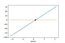
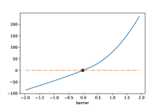
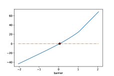
Case 1	Case 2	Case 3

Figure 2. Plot of $\hat{\rho}_{M}(b)$ for Case $i$ under the cost function $f_{i}$ as in (6.2), for $i=1,2,3$. The root (indicated by a star) becomes an approximation of the optimal barrier $b^{*}$.

With the approximated optimal barrier $b^{*}$, we shall now confirm the optimality by comparing the expected total costs $v_{b^{*}}$ with $v_{b}$ under suboptimal choices of $b$. In order to compute these, we continue using the set of paths $(\hat{\mathbf{X}},\hat{\mathbf{N}}^{\eta})$. Figure 3 shows the results. It can be confirmed that the selection $b^{*}$ indeed minimizes the total expected cost for all starting points.

Finally, we confirm the convergence as $\eta\to\infty$. In Figure 4, we plot the value function when $\eta=2,5,10,20,50,100,200,500,1000$ together with the classical case whose reflected path with lower barrier $b$ under $\mathbb{P}_{x}$ is approximated by $(\hat{X}_{n\Delta_{t}}^{(m)}+x)+\max_{0\leq l\leq n}(b-(\hat{X}_{l\Delta_{t}}^{(m)}+x))^{+}$. It is observed in all cases that the optimal barrier and the value function converge decreasingly to those of the classical case, confirming Theorem 5.1.

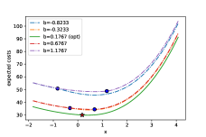
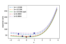
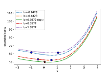
Case 1	Case 2	Case 3

Figure 3. Plot of the approximated value functions $v_{b^{*}}$ (solid) along with $v_{b}$ (dotted) for $b=b^{*}-1,b^{*}-0.5,b^{*}+0.5,b^{*}+1.0$ for Case $i$ for $i=1,2,3$. The points at the barriers are indicated by stars and circles for $b=b^{*}$ and $b\neq b^{*}$, respectively.

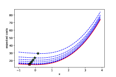
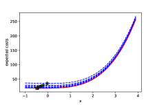
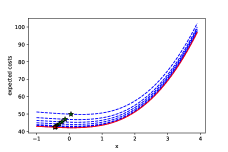
Case 1	Case 2	Case 3

Figure 4. Plot of the approximated value functions $v_{b^{*}}$ (dotted) for $\eta=2,5,10,20,50,100,200,500,1000$ along with that in the classical case (solid). The points at the barriers are indicated by stars.

Appendix A Proofs

A.1. The proof of Lemma 3.1

We fix $b,x\in\mathbb{R}$. Let $U^{b,\infty}$ and $R^{b,\infty}$ be those defined in Section 5 for the controlled and control processes in the classical setting under the barrier strategy with barrier $b$. First we have a bound

(A.1) $$X_{t}\leq U_{t}^{b}\leq U_{t}^{b,\infty},\quad 0\leq R^{b}_{t}\leq R^{b,\infty}_{t}.$$

By the convexity of $f$, we have $|f(U_{t}^{b})|\leq|f(U_{t}^{b,\infty})|+|f(X_{t})|+c$ where

(A.2) $$c=\begin{cases}|\inf_{y\in\mathbb{R}}f(y)|,\quad&\text{ if it exists},\\ 0,\quad&\text{ otherwise}.\end{cases}$$

By Remark 2.2 and [20, (A.3)] under Assumptions 2.1 and 2.2, we obtain (i). By (A.1) and since [20, Lemma 3] holds under Assumptions 2.1 and 2.2, we obtain (ii).

We have

(A.3) $$|v_{b}(x)|\leq\mathbb{E}_{x}\left[\int_{0}^{\infty}e^{-qt}(|f(X_{t})|+|f(U^{b,\infty}_{t})|{+c}){\rm d}t\right]+|C|\mathbb{E}_{x}\left[\int_{[0,\infty)}e^{-qt}{\rm d}R^{b,\infty}_{t}\right],$$

which is of polynomial growth by Remark 2.2 and the proof of [20, Lemma 3], showing (iii).

A.2. Proof of Lemma 3.2

Note that $T_{b}=T(k)$ for some $k\in\mathbb{N}$, almost surely on $\{T_{b}<\infty\}$. By the monotone convergence theorem and the strong Markov property, we have

(A.4) $$\lim_{\varepsilon\downarrow 0}\mathbb{P}_{x}\left(T_{b}=T_{b+\varepsilon},T_{b}<\infty\right)=\lim_{\varepsilon\downarrow 0}\sum_{k\in\mathbb{N}}\mathbb{P}_{x}\left(T_{b}=T_{b+\varepsilon}=T(k)\right)$$

(A.5) $$=\sum_{k\in\mathbb{N}}\lim_{\varepsilon\downarrow 0}\mathbb{P}_{x}\left(X_{T(1)}\geq b+\varepsilon,X_{T(2)}\geq b+\varepsilon,\dots,X_{T(k-1)}\geq b+\varepsilon,X_{T(k)}<b\right)$$

(A.6) $$=\sum_{k\in\mathbb{N}}\mathbb{P}_{x}\left(X_{T(1)}>b,X_{T(2)}>b,\dots,X_{T(k-1)}>b,X_{T(k)}<b\right)$$

(A.7) $$=\sum_{k\in\mathbb{N}}E^{(k)}(x),$$

where

(A.8) $$E^{(1)}(x)=\mathbb{P}_{x}\left(X_{T(1)}<b\right),\quad E^{(l+1)}(x)=\mathbb{E}_{x}\left[1_{\{X_{T(1)}>b\}}E^{(l)}(X_{T(1)})\right],\quad l\in\mathbb{N}.$$

By Remark 2.1, with $\{X_{T(1)}>b\}$ replaced by $\{X_{T(1)}\geq b\}$ in the definition of $E^{(k)}$ and going backwards from (A.7), we have $\lim_{\varepsilon\downarrow 0}\mathbb{P}_{x}\left(T_{b}=T_{b+\varepsilon},T_{b}<\infty\right)=\sum_{k\in\mathbb{N}}\mathbb{P}_{x}\left(T_{b}=T(k)\right)=\mathbb{P}_{x}\left(T_{b}<\infty\right)$.

On the other hand, by the monotone convergence theorem,

(A.9) $$\lim_{\varepsilon\downarrow 0}\mathbb{P}_{x}\left(T_{b}=T_{b-\varepsilon},T_{b}<\infty\right)=\sum_{k\in\mathbb{N}}\lim_{\varepsilon\downarrow 0}\mathbb{P}_{x}\left(X_{T(1)}\geq b,X_{T(2)}\geq b,\dots,X_{T(k-1)}\geq b,X_{T(k)}<b-\varepsilon\right)\\ =\sum_{k\in\mathbb{N}}\mathbb{P}_{x}\left(X_{T(1)}\geq b,X_{T(2)}\geq b,\dots,X_{T(k-1)}\geq b,X_{T(k)}<b\right)=\mathbb{P}_{x}(T_{b}<\infty).$$

Finally, because the map $b\mapsto T_{b}$ is nonincreasing, the proof is complete by monotone convergence.

A.3. Proof of Lemma 4.1

Since $f^{\prime}_{+}$ is nondecreasing, the function $\rho(b)=\mathbb{E}_{0}\left[\int_{0}^{\infty}e^{-qt}f^{\prime}_{+}(U^{0}_{t}+b){\rm d}t\right]$ is nondecreasing. By Corollary 3.1, monotone convergence, and Assumption2.1 (3), we have $\lim_{b\uparrow\infty}\rho(b)=f^{\prime}_{+}(\infty)/q>-C$ and $\lim_{b\downarrow-\infty}\rho(b)=f^{\prime}_{+}(-\infty)/q<-C$. In what follows we show the continuity of $\rho$.

(i) We first prove that the potential of the process $U^{b}$ does not have mass. Recall the first control time $T_{b}=T_{b}^{(1)}$. For $x,y,b\in\mathbb{R}$, we have

(A.10) $$\mathbb{E}_{x}\left[\int_{0}^{\infty}e^{-qt}1_{\{y\}}(U^{b}_{t}){\rm d}t\right]=\sum_{k\in\mathbb{N}}\mathbb{E}_{x}\left[\int_{T^{(k-1)}_{b}}^{T^{(k)}_{b}}e^{-qt}1_{\{y\}}(U^{b}_{t}){\rm d}t\right]$$

(A.11) $$=\mathbb{E}_{x}\left[\int_{0}^{T_{b}}e^{-qt}1_{\{y\}}(X_{t}){\rm d}t\right]+\sum_{k\in\mathbb{N}}\mathbb{E}_{x}\left[e^{-qT_{b}}\right]{\left(\mathbb{E}_{b}\left[e^{-qT_{b}}\right]\right)}^{k-1}\mathbb{E}_{b}\left[\int_{0}^{T_{b}}e^{-qt}1_{\{y\}}(X_{t}){\rm d}t\right],$$

which is equal to $0$ by Remark 2.1.

(ii) Since $f^{\prime}_{+}$ is right-continuous and by the dominated convergence theorem with Corollary 3.1, we have

(A.12) $$\rho(b+\varepsilon)-\rho(b)=\mathbb{E}_{0}\left[\int_{0}^{\infty}e^{-qt}(f^{\prime}_{+}(U^{0}_{t}+b+\varepsilon)-f^{\prime}_{+}(U^{0}_{t}+b)){\rm d}t\right]\xrightarrow{\varepsilon\downarrow 0}0.$$

Let $D$ be the set of discontinuous point of $f^{\prime}_{+}$ on $\mathbb{R}$, which is at most countable set since $f^{\prime}_{+}$ is nondecreasing. By Corollary 3.1 and the dominated convergence theorem, we have

$$\rho(b)-\rho(b-\varepsilon) ={\mathbb{E}_{0}\left[\int_{0}^{\infty}e^{-qt}(f^{\prime}_{+}(U^{0}_{t}+b)-f^{\prime}_{+}(U^{0}_{t}+b-\varepsilon)){\rm d}t\right]}$$

$$\xrightarrow{\varepsilon\downarrow 0}{\mathbb{E}_{0}\left[\int_{0}^{\infty}e^{-qt}\sum_{y\in D}(f^{\prime}_{+}(y)-f^{\prime}_{-}(y))1_{\{y\}}(U^{0}_{t}+b){\rm d}t\right]}$$

$${=\mathbb{E}_{b}\left[\int_{0}^{\infty}e^{-qt}\sum_{y\in D}(f^{\prime}_{+}(y)-f^{\prime}_{-}(y))1_{\{y\}}(U^{b}_{t}){\rm d}t\right],}$$

which is equal to $0$ since the potential of $U^{b}$ does not have mass as in (i).

A.4. Proof of Lemma 4.4

The proof is essentially the same as that of [20, Lemma 9] by simply replacing the classical reflected process $U^{b^{*},\infty}$ with the Poissonian version $U^{b^{*}}$. Following the same arguments, we obtain $v_{b^{\ast}}^{\prime\prime}(x)=\mathbb{E}_{x}\left[\int_{0}^{T_{b^{\ast}}}e^{-qt}f^{\prime\prime}(U^{b^{\ast}}_{t}){\rm d}t\right]$, which can be shown to be continuous by the dominated convergence theorem using the assumption that $f^{\prime\prime}$ is of polynomial growth, (3.12), and Lemma 3.2. For more details, see [20, Section A.6].

References

- [1] Albrecher, H., Ivanovs, J., Zhou, X. Exit identities for Lévy processes observed at Poisson arrival times. Bernoulli, 22, 1364–1382, 2016.
- [2] Avanzi, B., Cheung, E. C., Wong, B., Woo, J.K. On a periodic dividend barrier strategy in the dual model with continuous monitoring of solvency. Insurance Math. Econom., 52, 98–113, 2013.
- [3] Bensoussan, A., Tapiero, C.S. Impulsive control in management: prospects and applications. J. Optim. Theory Appl., 37(4), 419–442, 1982.
- [4] Benkherouf, L., Bensoussan, A. Optimality of an (s, S) policy with compound Poisson and diffusion demands: a quasi-variational inequalities approach. SIAM J. Control Optim., 48(2), 756–762, 2009
- [5] Bensoussan, A., Liu, R.H., Sethi S.P. Optimality of an (s, S) policy with compound Poisson and diffusion demands: a quasi-variational inequalities approach. SIAM J. Control Optim., 44(5), 1650–1676, 2005.
- [6] Bertoin, J. Lévy processes Cambridge University Press, 1996.
- [7] Biffis, E., Kyprianou, A.E. A note on scale functions and the time value of ruin for Lévy insurance risk processes. Insurance Math. Econom. , 46(1), 85–91, 2010.
- [8] Cai, N., Yang, X. International reserve management: A drift-switching reflected jump-diffusion model. Math. Financ., 28(1), 409–446, 2018.
- [9] Carr, P. Randomization and the American put. Rev. Financ. Stud., 11(3), 597-626, 1998.
- [10] Carr, P., Geman, H., Madan, D., Yor, M. The fine structure of asset returns: An empirical investigation. J. Bus., 75(2), 305–333, 2002.
- [11] Czarna, I., Palmowski, Z. Dividend problem with Parisian delay for a spectrally negative Lévy risk process. J. Optim. Theory Appl., 161(1), 239-256, 2014.
- [12] Hernández-Hernández, D., Pérez, J.L., Yamazaki, K. Optimality of refraction strategies for spectrally negative Lévy processes. SIAM J. Control Optim., 54(3), 1126–1156, 2016.
- [13] Jeanblanc-Picqué, M. Impulse control method and exchange rate. Math. Financ., 3(2), 161–177, 1993.
- [14] Kyprianou, A.E. Fluctuations of Lévy processes with applications. 2nd Edition Springer, Heidelberg, 2014.
- [15] Kyprianou, A. E., Loeffen, R. L. Refracted Lévy processes. Ann. inst. Henri Poincare (B) Probab. Stat., 46(1), 24–44, 2010.
- [16] Kyprianou, A. E., Pistorius, M. R. Perpetual options and Canadization through fluctuation theory. Ann. Appl. Probab., 13(3), 1077-1098, 2003.
- [17] Leung, T., Yamazaki, K., Zhang, H. An analytic recursive method for optimal multiple stopping: Canadization and phase-type fitting. Int. J. Theor. Appl. Finance, 18(05), 1550032, 2015.
- [18] Lkabous, M. A. Poissonian occupation times of spectrally negative Lévy processes with applications. Scandinavian Actuarial Journal, 2021(10), 916-935, 2021.
- [19] Mundaca, G., Øksendal, B. Optimal stochastic intervention control with application to the exchange rate. J. Math. Econ., 2(29), 225–243, 1998.
- [20] Noba, K and Yamazaki, K. On singular control for Lévy processes. Math. Oper. Res., published online, 2022.
- [21] Palmowski, Z., Pérez, J.L. Surya, B., Yamazaki, K. The Leland-Toft optimal capital structure model under Poisson observations. Finance Stoch., 24, 1035–1082, 2020.
- [22] Palmowski, Z., Pérez, J. L., Yamazaki, K. Double continuation regions for American options under Poisson exercise opportunities. Math. Financ., 31(2), 722-771. 2021.
- [23] Pérez, J.L., Yamazaki, K., Bensoussan, A. Optimal periodic replenishment policies for spectrally positive Lévy demand processes. SIAM J. Control Optim., 58(6), 3428–3456, 2020.
- [24] Pérez, J. L., Yamazaki, K., Yu, X. On the bail-out optimal dividend problem. J. Optim. Theory Appl., 179(2), 553-568, 2018.
- [25] Yamazaki, K. Inventory control for spectrally positive Lévy demand processes. Math. Oper. Res., 42(1), 212–237, 2017.
- [26] Zhao, Y., Chen, P., Yang, H. Optimal periodic dividend and capital injection problem for spectrally positive Lévy processes. Insurance Math. Econom. , 74, 135-146, 2017.
- [27] Zhao, Y., Wang, R., Yao, D., Chen, P. Optimal dividends and capital injections in the dual model with a random time horizon. J. Optim. Theory Appl., , 167(1), 272-295, 2015.