Posterior samples of source galaxies in strong gravitational lenses with score-based priors

Abstract

Inferring accurate posteriors for high-dimensional representations of the brightness of gravitationally-lensed sources is a major challenge, in part due to the difficulties of accurately quantifying the priors. Here, we report the use of a score-based model to encode the prior for the inference of undistorted images of background galaxies. This model is trained on a set of high-resolution images of undistorted galaxies. By adding the likelihood score to the prior score and using a reverse-time stochastic differential equation solver, we obtain samples from the posterior. Our method produces independent posterior samples and models the data almost down to the noise level. We show how the balance between the likelihood and the prior meet our expectations in an experiment with out-of-distribution data.

1 Introduction

Strong gravitational lensing – extreme distortions in the images of distant sources by the gravity of foreground lensing galaxies – is a powerful tool that can be used to probe the fundamental nature of dark matter, infer the expansion rate of the universe, and study the birth and evolution of nascent galaxies [1]. Inferring the spatial distribution of mass in the foreground lens and the spatial distribution of surface brightness in the background source is an essential component of achieving these scientific goals.

In this work, we ask the question: given a noisy image of a distorted source and the distribution of mass in the lensing galaxy, how can we infer the spatial distribution of surface brightness in the background source? The goal is to sample the posterior $p(\mathbf{x}\mid\mathbf{y},\mathbf{\kappa})$, where $\mathbf{x}$ are the variables representing the surface brightness distribution in the background source, $\mathbf{y}$ is the observed data, and $\mathbf{\kappa}$ are the variables representing the spatial distribution of mass in the lens.

In noisy and low-resolution data, the source can often be well-described by low-dimensional representations like the Sérsic profile [2, 3]. Through their functional forms, these representations implicitly impose a strong prior on the surface brightness. Higher-quality data, however, reveal rich and complex morphologies, which demand more expressive source models, such as a set of pixels [4, 5], allowing arbitrarily-complex representations at a finite resolution. These methods require priors that limit $\mathbf{x}$ to physically-plausible configurations to avoid unphysical source reconstructions caused by overfitting to noise. Such priors have typically taken heuristic and simplistic forms to facilitate calculations, such as gradient or curvature penalties [5]. Other expressive source models apply similar methods on adaptive grids [6, 7], decompose the source as a linear combination of shapelets [8, 9] or wavelets [10], or model the source as an approximate Gaussian process [11]. However, these priors are inaccurate since sampling from them does not yield galaxy-like images, which can bias lensing inference.

Recent work has explored the use of machine learning to create better source brightness priors for lensing inference, such as variational autoencoders [12], recurrent inference machines [13, 14, 15], and continuous neural fields [16]. These methods respectively have trouble accurately representing the prior over galaxy images, only produce maximum a posteriori parameter estimates, and only implicitly define a prior through the choice of a neural network architecture. Also, denoising diffusion probabilistic models [17, 18] have been applied to learn priors over galaxies outside the context of lensing inference [19].

In this work we use score-based modeling, formulated in terms of stochastic differential equations (SDEs)stochastic differential equation (SDE), to learn a highly-accurate prior over the source surface brightness for lensing analysis. In combination with a likelihood, this allows us to produce source posterior samples of remarkably high quality using SDE solvers. A similar approach was adopted in Remy et al. [20] to produce samples from the posterior of convergence maps from weak lensing data. These samples enable us to assess the significance of reconstructed source features. Our experiments show how our prior is balanced against the likelihood to enforce that reconstructions to look like training set galaxies in the low-signal-to-noise (SNR) regime. This represents a significant step towards accurate inference in high-dimensional spaces.

2 Inference of underconstrained variables with score-based priors

The data-generating process of strongly-lensed images of background galaxies can be described by the linear equation

$$\mathbf{y}=A\mathbf{x}+\boldsymbol{\eta}\,,$$ (1)

where $\mathbf{x}\in\mathbb{R}^{n}$ contains pixel intensities of the undistorted background source image, $A\in\mathbb{R}^{m\times n}$ encodes the lensing distortions (and thus a function of $\kappa$), interpolation over $\mathbf{x}$ and instrumental effects such as a point spread function, and $\boldsymbol{\eta}\in\mathbb{R}^{m}$ is additive instrumental noise, here assumed to be distributed as $\mathcal{N}(\mathbf{0},\sigma_{\mathcal{N}}^{2}\text{1})$. Since we consider the case where $\kappa$ is known, in our notation we drop the dependence on $A$ (or $\kappa$) and treat it as a known constant. The likelihood for the data given the source image is therefore $p(\mathbf{y}\mid\mathbf{x})=\mathcal{N}(\mathbf{y}\mid A\mathbf{x},\sigma_{\mathcal{N}}^{2}\text{1})$.

Our aim is to sample the posterior $p(\mathbf{x}\mid\mathbf{y})$, which, by Bayes’ theorem, is proportional to the product between the likelihood $p(\mathbf{y}\mid\mathbf{x})$ and a prior $p(\mathbf{x})$. Applying the logarithm thus gives

$$\log p(\mathbf{x}\mid\mathbf{y})=\log p(\mathbf{y}\mid\mathbf{x})+\log p(\mathbf{x})-\log p(\mathbf{y})\,.$$ (2)

The prior effectively gives the probability that any image $\mathbf{x}$ looks like a galaxy in the absence of a lensed observation $\mathbf{y}$. Recent advances in generative modeling have shown that the score of the prior, $\gradient_{\mathbf{x}}\log p(\mathbf{x})$, can be accurately learned from training data and sampled from using score-based modeling [21, 17, 18, 22]. We now summarize how to train a model $s_{\theta}(\mathbf{x})$ to approximate $\gradient_{\mathbf{x}}\log p(\mathbf{x})$ using score matching and our posterior sampling procedure.

2.1 Score matching

Score matching [23] is the task of training a model, $\mathbf{s}_{\theta}(\mathbf{x}):\mathbb{R}^{n}\rightarrow\mathbb{R}^{n}$, to match the score of a probability distribution, $\gradient_{\mathbf{x}}\log p(\mathbf{x})$. We use denoising score matching (DSM) [21, 24], which lets us learn an implicit distribution by training a network $\mathbf{s}_{\theta}(\mathbf{x})$ to remove Gaussian noise added to i.i.d. samples from that distribution. We follow previous works [25, 26, 22] in averaging the DSM loss over various scales $\sigma(t)$, here indexed by a continuous time variable $t\in[0,1]$, and conditioning the score model on this time index, $s_{\theta}(\mathbf{x},t)=\boldsymbol{\epsilon}_{\theta}(\mathbf{x},t)/\sigma(t)$, where $\boldsymbol{\epsilon}_{\theta}$ is the neural network. The loss is obtained by sampling uniformly over $t$, perturbing a training sample by adding noise of the corresponding scale, noted by $\sigma(t)\mathbf{z}$ with $\mathbf{z}\sim\mathcal{N}(\mathbf{0},\text{1})$, and computing the Fisher divergence between the model and the kernel of the perturbation:

$$\mathcal{L}_{\theta}=\mathbb{E}_{t\sim\mathcal{U}(0,1)}\mathbb{E}_{\mathbf{x}\sim\mathcal{D}}\mathbb{E}_{\mathbf{z}\sim\operatorname*{\mathcal{N}}(\mathbf{0},\text{1})}\left[\left\lVert\boldsymbol{\epsilon}_{\theta}\left(\mathbf{x}+\sigma(t)\,\mathbf{z},t\right)+\mathbf{z}\right\rVert_{2}^{2}\right]\,.$$ (3)

This loss is designed to address the manifold hypothesis [24, 25] and is related to denoising diffusion approaches that rely on a variational formulation [27, 17, 28, 25, 18, 29] to generate data with a fixed number of steps, unlike MCMC approaches.

More specifically, DSM can be phrased in terms of SDE s [22], where training data is evolved into noise under a variance-exploding diffusion process $\differential\mathbf{x}=g(t)\,\differential\mathbf{w}$. Here $g(t)$ is called the diffusion coefficient, $\mathbf{w}$ is a Wiener process and $t\in[0,1]$. The score-based model (SBM) learned using the DSM loss approximates the score $\gradient_{\mathbf{x}}\log p_{t}(\mathbf{x})$ induced by this SDE. The distribution $p_{t}(\mathbf{x})$ can be understood as the marginal distribution of trajectories from the SDE evolved up to time $t$. Samples from the distribution $p(\mathbf{x})=p_{0}(\mathbf{x})$ can then be generated by substituting this learned score into the corresponding reverse-time SDE [30] $\differential\mathbf{x}=-g^{2}(t)\gradient_{\mathbf{x}}\log p_{t}(\mathbf{x})\differential t+g(t)\,\differential\bar{\mathbf{w}}$ and solving it with the distribution initialized to a wide Gaussian, $p_{1}(\mathbf{x})=\operatorname*{\mathcal{N}}(\mathbf{x}|\mathbf{0},\sigma_{\mathrm{max}})$. Here $\bar{\mathbf{w}}$ is a reverse-time Wiener process and $\differential t$ is now an infinitesimal negative timestep.

2.2 Sampling from the posterior

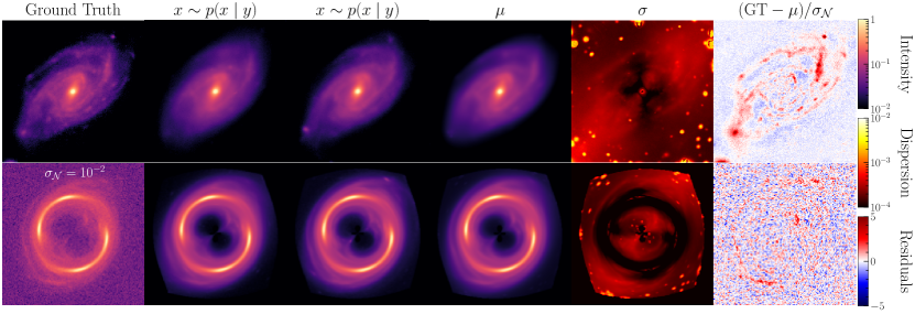
Figure 1: Source and observation reconstruction using $8000$ steps of the Euler-Maruyama solver. The first column shows the true source image and the observation, labeled with the noise level $\sigma_{\mathcal{N}}$. The other columns, from left to right, show two samples from the posterior, the mean and standard deviation of $320$ posterior samples, and the SNR of the residuals in the source plane (first row) and lens plane (second row). The residuals in the source plane are shown for illustrative purposes only since the accuracy with which we expect the source to be reconstructed is position-dependent.

Sampling from the posterior $p(\mathbf{x}\mid\mathbf{y})$ requires changing the $t=0$ boundary condition of the forward SDE from the prior $p(\mathbf{x})$ to the posterior $p(\mathbf{x}\mid\mathbf{y})$. This modifies the reverse-time SDE to read as [22]

$$\differential\mathbf{x}=-g^{2}(t)\gradient_{\mathbf{x}}\log p_{t}(\mathbf{x}\mid\mathbf{y})\differential t+g(t)\,\differential\bar{\mathbf{w}}\,.$$ (4)

Solving this equation until $t=0$ then yields independent samples from $p(\mathbf{x}\mid\mathbf{y})$. We can further apply Bayes’ rule to simplify the score in the above equation as

$$\gradient_{\mathbf{x}}\log p_{t}(\mathbf{x}\mid\mathbf{y})=\gradient_{\mathbf{x}}\log p_{t}(\mathbf{x})+\gradient_{\mathbf{x}}\log p_{t}(\mathbf{y}\mid\mathbf{x})\,.$$ (5)

The first term in this sum is modeled by our SBM, $s_{\theta}(\mathbf{x}_{t},t)$. We approximate the second using the convolved likelihood, $p_{t}(\mathbf{y}\mid\mathbf{x})\approx\operatorname*{\mathcal{N}}(\mathbf{y}\mid A\mathbf{x},(\sigma_{\mathcal{N}}^{2}+\sigma^{2}(t))\text{1})$. Intuitively, this can be understood as arising from the convolution of the Gaussian diffusion $\mathcal{N}(\mathbf{0},\,\sigma^{2}(t)\text{1})$ with the Gaussian likelihood $p(\mathbf{y}\mid\mathbf{x})$. We derive the convolved likelihood in more detail in appendix A.

With this machinery in place, we can apply the Euler-Maruyama solver (see e.g. [31]) to generate posterior samples of $\mathbf{x}$. The quality of the resulting samples is controlled by the number of time discretizations, $N$. We choose $N=8000$ based on Technique 2 of Song and Ermon [32]’s work, which we discuss in more detail in appendix B. This theory ensures that the samples from each iteration of the solver do not stray far from the high-density region of $p_{t}(\mathbf{x})$. The noise schedule in the DSM loss (or equivalently the diffusion coefficient in the forward SDE) employed in this work corresponds to the variance-exploding SDE (VE SDE) from Song et al. [22]. This amounts to setting $g(t)=\sqrt{\derivative*{\sigma^{2}(t)}{t}}$ with $\sigma(t)=\sigma_{\mathrm{min}}\left(\sigma_{\mathrm{max}}/\sigma_{\mathrm{min}}\right)^{t}$. We explain how $\sigma_{\mathrm{min/max}}$ is selected in section 3.

3 Results and conclusions

Figure 2: Application of the method to a lensing system with a highly out-of-distribution source. The ground truth is given in the leftmost panel. Other panels show increasingly noisy data (lower row) and a sample from their corresponding source posterior (upper row). As the likelihood becomes less informative, the prior dominates, making the sources increasingly look like galaxies.

To test our method, we trained our SBM on the PROBES dataset [33, 34], a high-quality sample of $2059$ galaxies with $256\times 256$ pixels. We used the data normalization scheme described in sec. 3.1 of Smith et al. [19]. For the SDE parameters we set $\sigma_{\mathrm{max}}=263.4$ (our estimation of the largest Euclidean distance between any two pairs in our training set [32]) and chose $\sigma_{\mathrm{min}}=10^{-4}$, roughly the scale of the smallest details in the training images. Our network is the reference PyTorch [35] implementation of NCSN++ architecture from Song et al. [22]. Training was carried out on four NVIDIA V100 GPUs, with a batch size of $16$, for a total of $\sim 350\,000$ optimization steps ($\sim 70$ hours wall-time). The results shown in fig. 1 are in the $g$ band (though in principle our framework can be extended to multiband data). The lens deflections are modeled using a singular isothermal ellipsoid (SIE) (see e.g. [36]) plus external shear. We produce noise-free images at $256\times 256$ resolution by ray-tracing and bilinearly-interpolating the source over the deflected coordinates. We then pixelate at $128\times 128$ resolution with average pooling. For sampling, we use 80 V100 GPUs in parallel, yielding $320$ samples in less than one hour (wall-time).

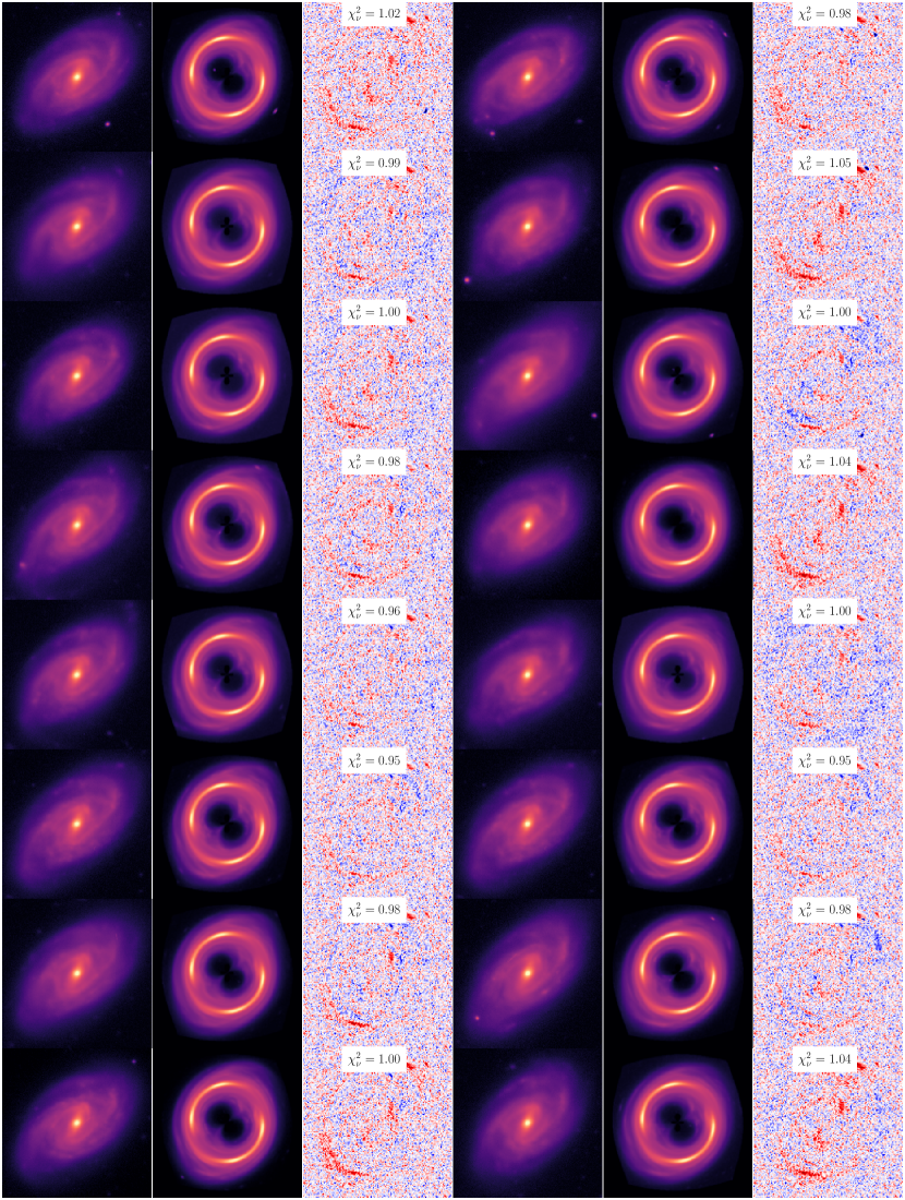
Figure 3: Additional posterior samples for the observation from fig. 1 in the source and lens planes, along with the $\chi^{2}_{\nu}$ of the residuals in the lens plane. The noise level in the data is $\sigma_{\mathcal{N}}=0.01$.

In fig. 1 we apply our method to a simulated lens from our test set. We show two posterior samples to give a sense of their variations, along with the mean and standard deviation calculated using $320$ samples; see fig. 3 for more samples. We find individual reconstructions and their mean match the observation almost down to the noise level. In the source plane, the bright core, spiral arms, and small but sharp clumps are well-reconstructed. Other small-scale features differ between the samples and have larger reconstruction uncertainties. The map of the standard deviation of the samples clearly shows fewer variations close to the diamond caustic, which matches our expectations, since these regions are highly magnified and thus better constrained. We find some posterior samples have bright peripheral spots, showing the model has learned they are present in the prior and that the approximation in our posterior sampling procedure does not suppress them.

Next, we apply our method to reconstructing an extremely out-of-distribution source. The results are shown in fig. 2. For low-noise observations, where the likelihood is highly informative, the model yields excellent reconstructions, capturing even small-scale spots in the source. This demonstrates that the model is qualitatively robust to distributional shifts when the likelihood is highly informative. With increasing noise levels the likelihood becomes less informative and the reconstructions increasingly resemble samples from the prior. As expected, the highly magnified regions in the center of the image (near the caustics) are better constrained.

In conclusion, we combined a score-based model trained on images of real galaxies with a differentiable lensing likelihood to sample posteriors of pixelated sources in strong lenses. Our posterior samples have remarkably high fidelity to the ground truth, and our reconstructed observations are consistent with the true ones almost down to the noise level. The independent samples generated from the posterior allow us to assess the confidence of any features in the reconstructions (e.g., the existence of a spiral arm) by examining their variations in them. Through our experiment with out-of-distribution sources, we showed that our model can recover these sources when high-quality data make the likelihood informative and can converge to the learned prior when the likelihood is not constraining. We believe this inference approach will help enable new scientific analysis using existing and upcoming strong lensing observations.

Broader Impact

The focus of this work is the rigorous estimation of uncertainties (posterior sampling) in high-dimensional spaces. The work can have an important cross-disciplinary impact on the application of machine learning in other natural sciences where accurate estimation of uncertainties is crucial. Given the striking nature of gravitational lensing images, we also believe that there is potential for a positive impact that will inspire broader interest in astrophysics. While we do not anticipate our work could have direct negative consequences, it could conceivably be applied to ethically-questionable inference problems. Additionally, users of such methods must be aware of their approximations and biases when applying them to scientific problems.

Checklist

1. For all authors…

   1. Do the main claims made in the abstract and introduction accurately reflect the paper’s contributions and scope? [Yes]

   2. Did you describe the limitations of your work? [Yes] We explain our convolved likelihood approximation in section 2.2 and study its validity in appendix A.

   3. Did you discuss any potential negative societal impacts of your work? [Yes] We address this in the "Broader Impacts" section.

   4. Have you read the ethics review guidelines and ensured that your paper conforms to them? [N/A]

2. If you are including theoretical results…

   1. Did you state the full set of assumptions of all theoretical results? [Yes] Please refer again to section 2.2 and appendix A

   2. Did you include complete proofs of all theoretical results? [N/A]

3. If you ran experiments…

   1. Did you include the code, data, and instructions needed to reproduce the main experimental results (either in the supplemental material or as a URL)? [No]

   2. Did you specify all the training details (e.g., data splits, hyperparameters, how they were chosen)? [Yes] We explain how we preprocess the data, set up our SDE and train our networks in section 3. Our networks and training setup is practically identical to the one in Song et al. [22], with the exception of the smaller batch size, as mentioned in the text.

   3. Did you report error bars (e.g., with respect to the random seed after running experiments multiple times)? [Yes] Our main result is careful quantification of uncertainties when solving an inverse problem.

   4. Did you include the total amount of compute and the type of resources used (e.g., type of GPUs, internal cluster, or cloud provider)? [Yes] Please see section 3. We acknowledge our computing cluster in the acknowledgements section.

4. If you are using existing assets (e.g., code, data, models) or curating/releasing new assets…

   1. If your work uses existing assets, did you cite the creators? [Yes] We reference the codebase from which we adapted our networks in section 3.

   2. Did you mention the license of the assets? [Yes] Please refer to the footnote on page 3.

   3. Did you include any new assets either in the supplemental material or as a URL? [No]

   4. Did you discuss whether and how consent was obtained from people whose data you’re using/curating? [N/A]

   5. Did you discuss whether the data you are using/curating contains personally identifiable information or offensive content? [N/A]

5. If you used crowdsourcing or conducted research with human subjects…

   1. Did you include the full text of instructions given to participants and screenshots, if applicable? [N/A]

   2. Did you describe any potential participant risks, with links to Institutional Review Board (IRB) approvals, if applicable? [N/A]

   3. Did you include the estimated hourly wage paid to participants and the total amount spent on participant compensation? [N/A]

Appendix A The convolved likelihood

In this appendix, we explain the origin of the convolved likelihood approximation to $\log p_{t}(\mathbf{y}\mid\mathbf{x}_{t})$ and demonstrate its regime of validity in the context of strong lensing source reconstruction. Let the Markov chain of the forward VE SDE be denoted as $\{\mathbf{X}_{t}\}_{t\in[0,1]}$. Our goal is to find a tractable expression for the marginal posterior $p_{t}(\mathbf{x}_{t}\mid\mathbf{y})$ at time $t$, the score of which is required to solve our reverse-time SDE. By construction of the VE SDE, the random variable $\mathbf{X}_{t}=\mathbf{X}_{0}+\mathbf{Z}_{t}$ can be expressed as the sum of the random variable $\mathbf{X}_{0}$, sampled from the posterior $\mathbf{x}_{0}\sim p(\mathbf{x}_{0}\mid\mathbf{y})$, and $\mathbf{Z}_{t}$, a noise perturbation $\mathbf{z}_{t}\sim\operatorname*{\mathcal{N}}(\mathbf{0},\Sigma_{t})$, where $\Sigma_{t}:=\sigma^{2}(t)\text{1}$. This implies the marginal posterior we seek can be written as the convolution

$$p_{t}(\mathbf{x}_{t}\mid\mathbf{y})=\int\differential{\mathbf{x}_{0}}p(\mathbf{x}_{0}\mid\mathbf{y})\,\operatorname*{\mathcal{N}}(\mathbf{x}_{t}\mid\mathbf{x}_{0},\Sigma_{t})\,.$$ (6)

We can expand this expression by applying Bayes’ rule to the first term in the integrand:

$$p_{t}(\mathbf{x}_{t}\mid\mathbf{y}) =\frac{1}{p(\mathbf{y})}\int\differential{\mathbf{x}_{0}}p(\mathbf{y}\mid\mathbf{x}_{0})\,p(\mathbf{x}_{0})\,\operatorname*{\mathcal{N}}(\mathbf{x}_{t}\mid\mathbf{x}_{0},\Sigma_{t})$$ (7)

$$=\frac{1}{p(\mathbf{y})}\int\differential{\mathbf{x}_{0}}\operatorname*{\mathcal{N}}(\mathbf{y}\mid A\mathbf{x}_{0},\Sigma_{y})\,p(\mathbf{x}_{0})\,\operatorname*{\mathcal{N}}(\mathbf{x}_{t}\mid\mathbf{x}_{0},\Sigma_{t})\,,$$ (8)

where we used the form of the lensing data generation process (eq. 1) to obtain the second line, with $\Sigma_{y}:=\sigma_{\mathcal{N}}^{2}\text{1}$. Given a sufficiently broad prior $p(\mathbf{x}_{0})$, the integral approximately factorizes into the product of the prior and likelihood convolved with the noise perturbation:

$$p_{t}(\mathbf{x}_{t}\mid\mathbf{y}) \approx\frac{1}{p(\mathbf{y})}\left[\int\differential{\mathbf{x}_{0}}\operatorname*{\mathcal{N}}(\mathbf{y}\mid A\mathbf{x}_{0},\Sigma_{y})\,\operatorname*{\mathcal{N}}(\mathbf{x}_{t}\mid\mathbf{x}_{0},\Sigma_{t})\right]\left[\int\differential{\mathbf{x}_{0}}p(\mathbf{x}_{0})\,\operatorname*{\mathcal{N}}(\mathbf{x}_{t}\mid\mathbf{x}_{0},\Sigma_{t})\right]$$ (9)

$$=\frac{1}{p(\mathbf{y})}\left[\int\differential{\mathbf{x}_{0}}\operatorname*{\mathcal{N}}(\mathbf{y}\mid A\mathbf{x}_{0},\Sigma_{y})\,\operatorname*{\mathcal{N}}(\mathbf{x}_{t}\mid\mathbf{x}_{0},\Sigma_{t})\right]p_{t}(\mathbf{x}_{t})$$ (10)

$$=\frac{\operatorname*{\mathcal{N}}(\mathbf{y}\mid A\mathbf{x}_{t},\Sigma_{y}+A\Sigma_{t}A^{T})\,p_{t}(\mathbf{x}_{t})}{p(\mathbf{y})}\,,$$ (11)

where we applied the definition of $p_{t}(\mathbf{x}_{t})$ to obtain the second equation and analytically evaluated the remaining integral (see e.g. sec. 3.3.1 of Murphy [45] for the required identity). By expanding the left-hand side of this equation with Bayes’ rule, we obtain the convolved likelihood,

$$p_{t}(\mathbf{y}\mid\mathbf{x}_{t})\approx\operatorname*{\mathcal{N}}(\mathbf{y}\mid A\mathbf{x}_{t},\Sigma_{y}+A\Sigma_{t}A^{T})\,.$$ (12)

We can examine the accuracy of the convolved likelihood factorization by considering the case where $p(\mathbf{x}_{0})=\operatorname*{\mathcal{N}}(\mathbf{x}_{0}\mid\mathbf{0},\Sigma_{x_{0}})$. In this case the integral in eq. 8 giving the marginal posterior can be evaluated analytically:

$$p_{t}(\mathbf{x}_{t}\mid\mathbf{y}) =\frac{1}{p(\mathbf{y})}\int\differential{\mathbf{x}_{0}}p(\mathbf{y}\mid\mathbf{x}_{0})\,p(\mathbf{x}_{0})\,p(\mathbf{x}_{t}\mid\mathbf{x}_{0})$$ (13)

$$=\frac{1}{p(\mathbf{y})}\int\differential{\mathbf{x}_{0}}\operatorname*{\mathcal{N}}(\mathbf{y}\mid A\mathbf{x}_{0},\Sigma_{y})\,\operatorname*{\mathcal{N}}(\mathbf{x}_{0}\mid\mathbf{0},\Sigma_{x_{0}})\,\operatorname*{\mathcal{N}}(\mathbf{x}_{t}\mid\mathbf{x}_{0},\Sigma_{t})$$ (14)

$$=\frac{\operatorname*{\mathcal{N}}(\mathbf{x}_{t}\mid\mathbf{0},\Sigma_{x_{0}}+\Sigma_{t})}{p(\mathbf{y})}\int\differential{\mathbf{x}_{0}}\operatorname*{\mathcal{N}}(\mathbf{y}\mid A\mathbf{x}_{0},\Sigma_{y})\,\operatorname*{\mathcal{N}}(\mathbf{x}_{0}\mid\mathbf{m}_{c},\Sigma_{c})$$ (15)

$$=\frac{\operatorname*{\mathcal{N}}(\mathbf{x}_{t}\mid\mathbf{0},\Sigma_{x_{0}}+\Sigma_{t})\,\operatorname*{\mathcal{N}}(\mathbf{y}\mid A\mathbf{m}_{c},\Sigma_{y}+A\Sigma_{c}A^{T})}{p(\mathbf{y})}\,,$$ (16)

where we obtained eq. 16 by simplifying the product of the last two terms in the integrand using eq. 371 from Petersen et al. [46] and defined

$$\Sigma_{c}:=(\Sigma_{x_{0}}^{-1}+\Sigma_{t}^{-1})^{-1}\,,\mbox{\quad\quad}\mathbf{m}_{c}:=\Sigma_{c}\Sigma_{t}^{-1}\mathbf{x}_{t}\,.$$

On the other hand, evaluating the integral $p_{t}(\mathbf{x})$ in our convolved likelihood factorization eq. 11 yields

$$p_{t}(\mathbf{x}_{t}\mid\mathbf{y}) \approx\frac{\operatorname*{\mathcal{N}}(\mathbf{x}_{t}\mid\mathbf{0},\Sigma_{x_{0}}+\Sigma_{t})\,\operatorname*{\mathcal{N}}(\mathbf{y}\mid A\mathbf{x}_{t},\Sigma_{y}+A\Sigma_{t}A^{T})}{p(\mathbf{y})}\,.$$ (17)

Thus, our approximation for the convolved likelihood holds if ${\operatorname*{\mathcal{N}}(\mathbf{y}\mid A\mathbf{m}_{c},\Sigma_{y}+A\Sigma_{c}A^{T})\approx\operatorname*{\mathcal{N}}(\mathbf{y}\mid A\mathbf{x}_{t},\Sigma_{y}+A\Sigma_{t}A^{T})}$. Such an approximation is valid when the prior $p(\mathbf{x}_{0})$ is broad compared to the likelihood. To test this, we expand $\Sigma_{c}$ in a Neumann series around $\Sigma_{t}$:

$$\Sigma_{c}=\Sigma_{t}-\Sigma_{t}\Sigma_{x_{0}}^{-1}\Sigma_{t}+\mathcal{O}(\lVert\Sigma_{t}(\Sigma_{x_{0}}^{-1}\Sigma_{t})^{2}\rVert_{2})\,,$$ (18)

where $\lVert\cdot\rVert_{2}$ is the spectral norm of a matrix, i.e. the magnitude of the largest eigenvalues of the covariance matrix. Our approximation holds when the second and higher order terms are negligible compared to the leading term in the expansion. We estimated the eigenvalues of $\Sigma_{x_{0}}$ by fitting a Gaussian random field on the PROBES dataset. Our estimate of the largest eigenvalue of $\Sigma_{x_{0}}$ is comparable to $\sigma_{\mathrm{max}}^{2}$, which means that our approximation might not hold for $t\lesssim 1$, but that it will be valid for most of the sampling procedure $0\leq t<1$. Moreover, it is worth noting that in the limit $t\rightarrow 0$, the approximation in eq. (12) becomes exact, and so the approximate SDE we are solving respects the same boundary condition as the exact SDE.

A final simplification we apply to our convolved likelihood to avoid an expensive matrix inversion at every step while solving the reverse-time SDE is to assume $AA^{T}\approx\text{1}$. Without this assumption, evaluating the convolved likelihood would require inverting the matrix $\Sigma_{y}+A\Sigma_{t}A^{T}$, the size of which is the number of pixels in the image squared. With this assumption, on the other hand, the covariance matrix of the convolved likelihood simplifies to $\Sigma_{y}+\Sigma_{t}\propto\text{1}$, which is trivial to invert. By examining $AA^{T}$ for different lens configurations, we find this is a reasonable approximation. In our checks, only a small fraction of off-diagonal elements are nonzero, and all diagonal elements are guaranteed to be no greater than $1$ since lensing conserves surface brightness. Consequentially, the final convolved likelihood we use for sampling is

$$p_{t}(\mathbf{y}\mid\mathbf{x}_{t})\approx\operatorname*{\mathcal{N}}(\mathbf{y}\mid A\mathbf{x}_{t},\Sigma_{y}+\Sigma_{t})\,.$$ (19)

Appendix B Euler-Maruyama discretization

The Euler-Maruyama discretization of the reverse-time SDE is

$$\mathbf{x}_{t+\Delta t}=\mathbf{x}_{t}-g^{2}(t)\gradient_{\mathbf{x}_{t}}\log p_{t}(\mathbf{x}_{t}\mid\mathbf{y})\Delta t+g(t)\mathbf{z}_{t}\sqrt{-\Delta t}$$ (20)

with $\mathbf{z}_{t}\sim\mathcal{N}(\mathbf{0},\text{1})$, $\Delta t=-1/N$ and $N$ the number of discretisations of the time index $t\in[0,1]$. In practice, we can choose $N$ to satisfy technique 2 of Song and Ermon [32], such that the discretized noise schedule used in our work $\sigma(t)=(\sigma_{\mathrm{max}}/\sigma_{\mathrm{min}})^{t}\sigma_{\mathrm{min}}$ is now a geometric progression with a ratio

$$\gamma=\frac{\sigma(t)}{\sigma(t+\Delta t)}=\left(\frac{\sigma_{\mathrm{max}}}{\sigma_{\mathrm{min}}}\right)^{1/N}\,.$$ (21)

The ratio $\gamma>1$ should be close enough to $1$ so that a sample from $p_{t}(\mathbf{x}_{t})$ should at least belong to the $3\sigma$ density region of $p_{t+\Delta t}(\mathbf{x}_{t})$. In such a situation, a sample from $p_{t}(\mathbf{x}_{t})$ will have some probability $p(N)$ of belonging to the $3\sigma$ density region of $p_{t+\Delta t}(\mathbf{x}_{t})$, meaning it is a likely sample even after a transition to the density distribution at lower temperature.

We follow Song and Ermon [32] in setting this probability to

$$p(N)=\Phi(\sqrt{2n}(\gamma-1)+3\gamma)-\Phi(\sqrt{2n}(\gamma-1)-3\gamma)$$ (22)

where $\Phi$ is the CDF of a normal distribution. For a stable diffusion, we ask that $p(N)\gtrsim 0.5$. For the dimensionality of our problem ($n=256^{2}$ for the PROBES dataset), we thus have that $N=2000$ minimally satisfy this criteria with $p(2000)=0.64$. We can increase our confidence in the solver by setting $N=8000$, s.t. $p(8000)=0.99$, which is what is used in this work.

Additional figures

References

- Treu [2010] Tommaso Treu. Strong Lensing by Galaxies. Annual Review of Astronomy and Astrophysics, 48:87–125, September 2010. doi: 10.1146/annurev-astro-081309-130924.
- Sérsic [1963] J. L. Sérsic. Influence of the atmospheric and instrumental dispersion on the brightness distribution in a galaxy. Boletin de la Asociacion Argentina de Astronomia La Plata Argentina, 6:41–43, February 1963.
- Spilker et al. [2016] J. S. Spilker, D. P. Marrone, M. Aravena, M. Béthermin, M. S. Bothwell, J. E. Carlstrom, S. C. Chapman, T. M. Crawford, C. de Breuck, C. D. Fassnacht, A. H. Gonzalez, T. R. Greve, Y. Hezaveh, K. Litke, J. Ma, M. Malkan, K. M. Rotermund, M. Strandet, J. D. Vieira, A. Weiss, and N. Welikala. ALMA Imaging and Gravitational Lens Models of South Pole Telescope—Selected Dusty, Star-Forming Galaxies at High Redshifts. Astrophysical Journal, 826(2):112, August 2016. doi: 10.3847/0004-637X/826/2/112.
- Warren and Dye [2003] S. J. Warren and S. Dye. Semilinear Gravitational Lens Inversion. Astrophysical Journal, 590(2):673–682, June 2003. doi: 10.1086/375132.
- Suyu et al. [2006] S. H. Suyu, P. J. Marshall, M. P. Hobson, and R. D. Blandford. A Bayesian analysis of regularized source inversions in gravitational lensing. Monthly Notices of the Royal Astronomical Society, 371(2):983–998, September 2006. doi: 10.1111/j.1365-2966.2006.10733.x.
- Vegetti and Koopmans [2009] S. Vegetti and L. V. E. Koopmans. Bayesian strong gravitational-lens modelling on adaptive grids: objective detection of mass substructure in Galaxies. Monthly Notices of the Royal Astronomical Society, 392(3):945–963, 01 2009. ISSN 0035-8711. doi: 10.1111/j.1365-2966.2008.14005.x. URL https://doi.org/10.1111/j.1365-2966.2008.14005.x.
- Nightingale and Dye [2015] J. W. Nightingale and S. Dye. Adaptive semi-linear inversion of strong gravitational lens imaging. Monthly Notices of the Royal Astronomical Society, 452(3):2940–2959, September 2015. doi: 10.1093/mnras/stv1455.
- Refregier [2003] Alexandre Refregier. Shapelets - I. A method for image analysis. Monthly Notices of the Royal Astronomical Society, 338(1):35–47, January 2003. doi: 10.1046/j.1365-8711.2003.05901.x.
- Birrer et al. [2015] Simon Birrer, Adam Amara, and Alexandre Refregier. Gravitational Lens Modeling with Basis Sets. Astrophysical Journal, 813(2):102, November 2015. doi: 10.1088/0004-637X/813/2/102.
- Galan et al. [2021] A. Galan, A. Peel, R. Joseph, F. Courbin, and J. L Starck. SLITronomy: towards a fully wavelet-based strong lensing inversion technique. Astron. Astrophys., 647:A176, 2021. doi: 10.1051/0004-6361/202039363.
- Karchev et al. [2022] Konstantin Karchev, Adam Coogan, and Christoph Weniger. Strong-lensing source reconstruction with variationally optimized Gaussian processes. Mon. Not. Roy. Astron. Soc., 512(1):661–685, 2022. doi: 10.1093/mnras/stac311.
- Coogan et al. [2020] Adam Coogan, Konstantin Karchev, and Christoph Weniger. Targeted Likelihood-Free Inference of Dark Matter Substructure in Strongly-Lensed Galaxies. arXiv e-prints, art. arXiv:2010.07032, October 2020.
- Morningstar et al. [2019] Warren R. Morningstar, Laurence Perreault Levasseur, Yashar D. Hezaveh, Roger Blandford, Phil Marshall, Patrick Putzky, Thomas D. Rueter, Risa Wechsler, and Max Welling. Data-driven reconstruction of gravitationally lensed galaxies using recurrent inference machines. The Astrophysical Journal, 883(1):14, sep 2019. doi: 10.3847/1538-4357/ab35d7. URL https://doi.org/10.3847/1538-4357/ab35d7.
- Morningstar et al. [2018] Warren R. Morningstar, Yashar D. Hezaveh, Laurence Perreault Levasseur, Roger D. Blandford, Philip J. Marshall, Patrick Putzky, and Risa H. Wechsler. Analyzing interferometric observations of strong gravitational lenses with recurrent and convolutional neural networks. 7 2018.
- Adam et al. [2022] Alexandre Adam, Laurence Perreault-Levasseur, and Yashar Hezaveh. Pixelated Reconstruction of Gravitational Lenses using Recurrent Inference Machines. arXiv e-prints, art. arXiv:2207.01073, July 2022.
- Mishra-Sharma and Yang [2022] Siddharth Mishra-Sharma and Ge Yang. Strong Lensing Source Reconstruction Using Continuous Neural Fields. arXiv e-prints, art. arXiv:2206.14820, June 2022.
- Sohl-Dickstein et al. [2015] Jascha Sohl-Dickstein, Eric Weiss, Niru Maheswaranathan, and Surya Ganguli. Deep unsupervised learning using nonequilibrium thermodynamics. In Francis Bach and David Blei, editors, Proceedings of the 32nd International Conference on Machine Learning, volume 37 of Proceedings of Machine Learning Research, pages 2256–2265, Lille, France, 07–09 Jul 2015. PMLR. URL https://proceedings.mlr.press/v37/sohl-dickstein15.html.
- Ho et al. [2020] Jonathan Ho, Ajay Jain, and Pieter Abbeel. Denoising diffusion probabilistic models. Neural Information Processing Systems (NeurIPS), 2020.
- Smith et al. [2022] Michael J Smith, James E Geach, Ryan A Jackson, Nikhil Arora, Connor Stone, and Stéphane Courteau. Realistic galaxy image simulation via score-based generative models. Monthly Notices of the Royal Astronomical Society, 511(2):1808–1818, jan 2022. doi: 10.1093/mnras/stac130. URL https://doi.org/10.1093%2Fmnras%2Fstac130.
- Remy et al. [2022] Benjamin Remy, Francois Lanusse, Niall Jeffrey, Jia Liu, Jean-Luc Starck, Ken Osato, and Tim Schrabback. Probabilistic Mass Mapping with Neural Score Estimation. arXiv e-prints, art. arXiv:2201.05561, January 2022.
- Vincent [2011] Pascal Vincent. A connection between score matching and denoising autoencoders. Neural Comput., 23(7):1661–1674, 2011. doi: 10.1162/NECO\_a\_00142. URL https://doi.org/10.1162/NECO_a_00142.
- Song et al. [2021] Yang Song, Jascha Sohl-Dickstein, Diederik P Kingma, Abhishek Kumar, Stefano Ermon, and Ben Poole. Score-based generative modeling through stochastic differential equations. In International Conference on Learning Representations, 2021. URL https://arxiv.org/abs/2011.13456.
- Hyvärinen [2005] Aapo Hyvärinen. Estimation of non-normalized statistical models by score matching. Journal of Machine Learning Research, 6(24):695–709, 2005. URL http://jmlr.org/papers/v6/hyvarinen05a.html.
- Alain and Bengio [2014] Guillaume Alain and Yoshua Bengio. What regularized auto-encoders learn from the data-generating distribution. J. Mach. Learn. Res., 15(1):3563–3593, jan 2014. ISSN 1532-4435.
- Song and Ermon [2019] Yang Song and Stefano Ermon. Generative modeling by estimating gradients of the data distribution. In Proceedings of the 33rd International Conference on Neural Information Processing Systems, Red Hook, NY, USA, 2019. Curran Associates Inc.
- Lim et al. [2020] Jae Hyun Lim, Aaron C. Courville, Christopher J. Pal, and Chin-Wei Huang. AR-DAE: towards unbiased neural entropy gradient estimation. In Proceedings of the 37th International Conference on Machine Learning, ICML 2020, 13-18 July 2020, Virtual Event, volume 119 of Proceedings of Machine Learning Research, pages 6061–6071. PMLR, 2020. URL http://proceedings.mlr.press/v119/lim20a.html.
- Bengio et al. [2014] Yoshua Bengio, Eric Laufer, Guillaume Alain, and Jason Yosinski. Deep generative stochastic networks trainable by backprop. In International Conference on Machine Learning, pages 226–234. PMLR, 2014.
- Goyal et al. [2017] Anirudh Goyal, Nan Rosemary Ke, Surya Ganguli, and Yoshua Bengio. Variational walkback: Learning a transition operator as a stochastic recurrent net. Advances in Neural Information Processing Systems, 30, 2017.
- Graikos et al. [2022] Alexandros Graikos, Nikolay Malkin, Nebojsa Jojic, and Dimitris Samaras. Diffusion models as plug-and-play priors. Neural Information Processing Systems (NeurIPS), 2022. To appear; arXiv preprint 2206.09012.
- Anderson [1982] Brian D.O. Anderson. Reverse-time diffusion equation models. Stochastic Processes and their Applications, 12(3):313–326, 1982. ISSN 0304-4149. doi: https://doi.org/10.1016/0304-4149(82)90051-5. URL https://www.sciencedirect.com/science/article/pii/0304414982900515.
- Kloeden and Platen [2011] P.E. Kloeden and E. Platen. Numerical Solution of Stochastic Differential Equations. Stochastic Modelling and Applied Probability. Springer Berlin Heidelberg, 2011. ISBN 9783540540625. URL https://books.google.ca/books?id=BCvtssom1CMC.
- Song and Ermon [2020] Yang Song and Stefano Ermon. Improved techniques for training score-based generative models. CoRR, abs/2006.09011, 2020. URL https://arxiv.org/abs/2006.09011.
- Stone and Courteau [2019] Connor Stone and Stéphane Courteau. The Intrinsic Scatter of the Radial Acceleration Relation. The Astrophysical Journal, 882(1):6, September 2019. doi: 10.3847/1538-4357/ab3126.
- Stone et al. [2021] Connor Stone, Stéphane Courteau, and Nikhil Arora. The Intrinsic Scatter of Galaxy Scaling Relations. The Astrophysical Journal, 912(1):41, May 2021. doi: 10.3847/1538-4357/abebe4.
- Paszke et al. [2019a] Adam Paszke, Sam Gross, Francisco Massa, Adam Lerer, James Bradbury, Gregory Chanan, Trevor Killeen, Zeming Lin, Natalia Gimelshein, Luca Antiga, Alban Desmaison, Andreas Kopf, Edward Yang, Zachary DeVito, Martin Raison, Alykhan Tejani, Sasank Chilamkurthy, Benoit Steiner, Lu Fang, Junjie Bai, and Soumith Chintala. Pytorch: An imperative style, high-performance deep learning library. In H. Wallach, H. Larochelle, A. Beygelzimer, F. d'Alché-Buc, E. Fox, and R. Garnett, editors, Advances in Neural Information Processing Systems 32, pages 8024–8035. Curran Associates, Inc., 2019a. URL http://papers.neurips.cc/paper/9015-pytorch-an-imperative-style-high-performance-deep-learning-library.pdf.
- Meneghetti [2021] Massimo Meneghetti. Introduction to Gravitational Lensing: With Python Examples, volume 956. Springer Nature, 2021.
- Ramesh et al. [2022] Aditya Ramesh, Prafulla Dhariwal, Alex Nichol, Casey Chu, and Mark Chen. Hierarchical Text-Conditional Image Generation with CLIP Latents. arXiv e-prints, art. arXiv:2204.06125, April 2022.
- Astropy Collaboration et al. [2013] Astropy Collaboration, T. P. Robitaille, E. J. Tollerud, P. Greenfield, M. Droettboom, E. Bray, T. Aldcroft, M. Davis, A. Ginsburg, A. M. Price-Whelan, W. E. Kerzendorf, A. Conley, N. Crighton, K. Barbary, D. Muna, H. Ferguson, F. Grollier, M. M. Parikh, P. H. Nair, H. M. Unther, C. Deil, J. Woillez, S. Conseil, R. Kramer, J. E. H. Turner, L. Singer, R. Fox, B. A. Weaver, V. Zabalza, Z. I. Edwards, K. Azalee Bostroem, D. J. Burke, A. R. Casey, S. M. Crawford, N. Dencheva, J. Ely, T. Jenness, K. Labrie, P. L. Lim, F. Pierfederici, A. Pontzen, A. Ptak, B. Refsdal, M. Servillat, and O. Streicher. Astropy: A community Python package for astronomy. Astronomy and Astrophysics, 558:A33, October 2013. doi: 10.1051/0004-6361/201322068.
- Astropy Collaboration et al. [2018] Astropy Collaboration, A. M. Price-Whelan, B. M. Sipőcz, H. M. Günther, P. L. Lim, S. M. Crawford, S. Conseil, D. L. Shupe, M. W. Craig, N. Dencheva, A. Ginsburg, J. T. Vand erPlas, L. D. Bradley, D. Pérez-Suárez, M. de Val-Borro, T. L. Aldcroft, K. L. Cruz, T. P. Robitaille, E. J. Tollerud, C. Ardelean, T. Babej, Y. P. Bach, M. Bachetti, A. V. Bakanov, S. P. Bamford, G. Barentsen, P. Barmby, A. Baumbach, K. L. Berry, F. Biscani, M. Boquien, K. A. Bostroem, L. G. Bouma, G. B. Brammer, E. M. Bray, H. Breytenbach, H. Buddelmeijer, D. J. Burke, G. Calderone, J. L. Cano Rodríguez, M. Cara, J. V. M. Cardoso, S. Cheedella, Y. Copin, L. Corrales, D. Crichton, D. D’Avella, C. Deil, É. Depagne, J. P. Dietrich, A. Donath, M. Droettboom, N. Earl, T. Erben, S. Fabbro, L. A. Ferreira, T. Finethy, R. T. Fox, L. H. Garrison, S. L. J. Gibbons, D. A. Goldstein, R. Gommers, J. P. Greco, P. Greenfield, A. M. Groener, F. Grollier, A. Hagen, P. Hirst, D. Homeier, A. J. Horton, G. Hosseinzadeh, L. Hu, J. S. Hunkeler, Ž. Ivezić, A. Jain, T. Jenness, G. Kanarek, S. Kendrew, N. S. Kern, W. E. Kerzendorf, A. Khvalko, J. King, D. Kirkby, A. M. Kulkarni, A. Kumar, A. Lee, D. Lenz, S. P. Littlefair, Z. Ma, D. M. Macleod, M. Mastropietro, C. McCully, S. Montagnac, B. M. Morris, M. Mueller, S. J. Mumford, D. Muna, N. A. Murphy, S. Nelson, G. H. Nguyen, J. P. Ninan, M. Nöthe, S. Ogaz, S. Oh, J. K. Parejko, N. Parley, S. Pascual, R. Patil, A. A. Patil, A. L. Plunkett, J. X. Prochaska, T. Rastogi, V. Reddy Janga, J. Sabater, P. Sakurikar, M. Seifert, L. E. Sherbert, H. Sherwood-Taylor, A. Y. Shih, J. Sick, M. T. Silbiger, S. Singanamalla, L. P. Singer, P. H. Sladen, K. A. Sooley, S. Sornarajah, O. Streicher, P. Teuben, S. W. Thomas, G. R. Tremblay, J. E. H. Turner, V. Terrón, M. H. van Kerkwijk, A. de la Vega, L. L. Watkins, B. A. Weaver, J. B. Whitmore, J. Woillez, V. Zabalza, and Astropy Contributors. The Astropy Project: Building an Open-science Project and Status of the v2.0 Core Package. Astronomical Journal, 156(3):123, September 2018. doi: 10.3847/1538-3881/aabc4f.
- Kluyver et al. [2016] Thomas Kluyver, Benjamin Ragan-Kelley, Fernando Pérez, Brian Granger, Matthias Bussonnier, Jonathan Frederic, Kyle Kelley, Jessica Hamrick, Jason Grout, Sylvain Corlay, Paul Ivanov, Damián Avila, Safia Abdalla, Carol Willing, and Jupyter development team. Jupyter notebooks ? a publishing format for reproducible computational workflows. In Fernando Loizides and Birgit Scmidt, editors, Positioning and Power in Academic Publishing: Players, Agents and Agendas, pages 87–90. IOS Press, 2016. URL https://eprints.soton.ac.uk/403913/.
- Hunter [2007] J. D. Hunter. Matplotlib: A 2d graphics environment. Computing in Science & Engineering, 9(3):90–95, 2007. doi: 10.1109/MCSE.2007.55.
- Harris et al. [2020] Charles R. Harris, K. Jarrod Millman, Stéfan J. van der Walt, Ralf Gommers, Pauli Virtanen, David Cournapeau, Eric Wieser, Julian Taylor, Sebastian Berg, Nathaniel J. Smith, Robert Kern, Matti Picus, Stephan Hoyer, Marten H. van Kerkwijk, Matthew Brett, Allan Haldane, Jaime Fernández del Río, Mark Wiebe, Pearu Peterson, Pierre Gérard-Marchant, Kevin Sheppard, Tyler Reddy, Warren Weckesser, Hameer Abbasi, Christoph Gohlke, and Travis E. Oliphant. Array programming with NumPy. Nature, 585(7825):357–362, September 2020. doi: 10.1038/s41586-020-2649-2. URL https://doi.org/10.1038/s41586-020-2649-2.
- Paszke et al. [2019b] Adam Paszke, Sam Gross, Francisco Massa, Adam Lerer, James Bradbury, Gregory Chanan, Trevor Killeen, Zeming Lin, Natalia Gimelshein, Luca Antiga, Alban Desmaison, Andreas Kopf, Edward Yang, Zachary DeVito, Martin Raison, Alykhan Tejani, Sasank Chilamkurthy, Benoit Steiner, Lu Fang, Junjie Bai, and Soumith Chintala. Pytorch: An imperative style, high-performance deep learning library. In H. Wallach, H. Larochelle, A. Beygelzimer, F. d'Alché-Buc, E. Fox, and R. Garnett, editors, Advances in Neural Information Processing Systems 32, pages 8024–8035. Curran Associates, Inc., 2019b. URL http://papers.neurips.cc/paper/9015-pytorch-an-imperative-style-high-performance-deep-learning-library.pdf.
- da Costa-Luis [2019] Casper O. da Costa-Luis. ‘tqdm‘: A fast, extensible progress meter for python and cli. Journal of Open Source Software, 4(37):1277, 2019. URL https://doi.org/10.21105/joss.01277.
- Murphy [2022] Kevin P. Murphy. Probabilistic Machine Learning: An introduction. MIT Press, 2022. URL probml.ai.
- Petersen et al. [2008] Kaare Brandt Petersen, Michael Syskind Pedersen, et al. The matrix cookbook. Technical University of Denmark, 7(15):510, 2008.