Magnetospheric Multiscale Observations of Markov Turbulence
on Kinetic Scales

Abstract

In our previous studies we have examined solar wind and magnetospheric plasmas turbulence, including Markovian character on large inertial magnetohydrodynamic scales. Here we present the results of statistical analysis of magnetic field fluctuations in the Earth’s magnetosheath based on Magnetospheric Multiscale mission at much smaller kinetic scales. Following our results on spectral analysis with very large slopes of about -16/3, we apply Markov processes approach to turbulence in this kinetic regime. It is shown that the Chapman-Kolmogorov equation is satisfied and the lowest-order Kramers-Moyal coefficients describing drift and diffusion with a power-law dependence are consistent with a generalized Ornstein-Uhlenbeck process. The solutions of the Fokker-Planck equation agree with experimental probability density functions, which exhibit a universal global scale invariance through the kinetic domain. In particular, for moderate scales we have the kappa distribution described by various peaked shapes with heavy tails, which with large values of kappa parameter are reduced to the Gaussian distribution for large inertial scales. This shows that the turbulence cascade can be described by the Markov processes also on very small scales. The obtained results on kinetic scales may be useful for better understanding of the physical mechanisms governing turbulence.

1 Introduction

Turbulence appears in many real systems in nature, including various fluids with the embedded magnetic fields (Frisch, 1995; Biskamp, 2003). In particular, space and astrophysical plasmas are natural laboratories for investigating the dynamics of turbulence (Chang, 2015; Bruno & Carbone, 2016; Echim et al., 2021). This is complex phenomenon that contains deterministic and random components. Therefore, besides the effort to describe this problem in terms of difference equations a statistical approach is also useful. The important question for any dynamical system is whether given a probability distribution of the characteristic property of a system in a given moment, one can determine statistical properties of this dynamical system in a future. Therefore, a concept of a Markov process in which the future statistics is independent of the past is an important issue also for turbulence (Pedrizzetti & Novikov, 1994). It is possible to prove the existence of a Markov process experimentally and furthermore to extract the differential equation for this Markov process directly from the measured data without using any assumptions or models for the underlying stochastic process (Renner et al., 2001). Strumik & Macek (2008a, b) have applied this statistical method to solar wind magnetic fluctuations in the inertial range. A similar approach has recently been applied to the Parker Solar Probe (PSP) mission in the solar wind at sub-proton scales (Benella et al., 2022).

Our previous studies have also dealt with turbulence in solar wind and magnetospheric plasmas on large-(inertial) magnetohydrodynamic scales, using observations by the Ulysses mission in the solar wind beyond the ecliptic plane (Wawrzaszek & Macek, 2010), and Voyager mission in the heliosphere and heliosheath (Macek et al., 2011, 2012) and even at the boundaries of the Solar System (Macek et al., 2014). Based on THEMIS mission in the Earth’s magnetosheath, we have also verified that turbulence at shocks is well described by inward and outward propagating Alfvén waves (Macek et al., 2015, 2017).

Here we consider again turbulence in the Earth’s magnetosheath, where timescales are much shorter than those in the heliosheath, but based on observations from the Magnetospheric Multiscale (MMS) mission on kinetic scales (Macek et al., 2018). In this case it is hotly debated whether the turbulence energy cascade results from the dissipation of the kinetic Alfvén waves (KAW) (e.g., Schekochihin et al., 2009). On the contrary, Papini et al. (2021) has recently argued that the turbulence energy at kinetic scales could not be related to KAW activity, but is mainly driven by localized nonlinear structures. Certainly, it is possible that the observed stochastic nature of fluctuations in the sub-ion scale could be due to the interaction between coherent structures (e.g. Chang, 2015; Echim et al., 2021), including local reconnection processes at kinetic scales (Macek et al., 2019a, b). Admittedly, the nature of wave modes in operation cannot be determined on the statistical analysis, but we hope that the Markov approach will provide a contact point with a dynamical system approach to turbulence and hence the results of this study will be useful in future investigations.

The data under study are briefly described in Section 2, with statistical methods outlined in Section 3. In Section 4 we present the results of our analysis, showing that the solutions of the Fokker-Planck equation agree well with experimental probability density functions. The importance of Markov processes for turbulence in space plasmas with a universal global scale invariance also through the kinetic domain is underlined in Section 5.

2 Data

The MMS mission was launched in 2015 to investigate plasma processes in the magnetosphere and the solar wind plasma especially on small scales (Burch et al., 2016). We analyze the statistics of the fluctuations of all components of the magnetic field $\mathbf{B}=(B_{x},B_{y},B_{z})$, with the total magnitude $B_{T}=|\mathbb{B}|$, in the Geocentric Solar Ecliptic (GSE) coordinates obtained from the FluxGate Magnetometers (FGM), see (Russell et al., 2016). We investigate BURST-type observations with the highest available resolution of $\Delta t_{B}$ = 7.8 ms, which corresponds to approximately 128 samples per second. Macek et al. (2018) have selected interval on 28 December 2015 from 01.48:04 to 01.52:59 with 37,856 measurement points for the magnetic field, which are available just behind the bow shock (BS). The position of MMS during this event within the Earth’s magnetosheath has been depicted in Figure 1, case (a) of Ref. (Macek et al., 2018). Admittedly, the highest-resolution BURST-type magnetic data $B$ are limited in time. This analysis has allowed us to go well beyond the kinetic regime, i.e., above the electron Taylor-shifted inertial frequency $f_{\lambda e}=(V/c)f_{pe}$, where $f_{pe}$ is plasma frequency ($V$ is the solar wind velocity and $c$ denotes the speed of light), at above $f_{\lambda e}\sim$ 20 Hz characterized by a steep spectrum with a slope of about -11/2, as seen in their Figure 2 (for details see Macek et al., 2018). Even though with lower resolution for the ion velocity $V$ the spectrum could only be resolved to the onset of kinetic scales at $\sim$2 Hz it is worth to investigate further this case in view of the Markov property of turbulence.

3 Methods

As usual we use the increments of any characteristic parameter $x$ describing a turbulent system

$$\delta x(t,\tau)=x(t+\tau)-x(t)$$ (1)

at each time $t$ and a given scale $\tau$. Following the well-known scenario the fluctuations $\delta x(t,\tau)$ in a larger scale are transferred to smaller and smaller scales $\tau$. In this way turbulence may be regarded as a stochastic process with $N$-point joint transition probability distribution $P(x_{1},\tau_{1}|x_{2},\tau_{2};\ldots;x_{N},\tau_{N})$, where $P(x_{i},\tau_{i}|x_{j},\tau_{j})=P(x_{i},\tau_{i};x_{j},\tau_{j})/P(x_{j},\tau_{j})$ is the conditional probability density function (PDF). The process is Markovian if the $N$-point joint transition probability distribution is completely determined by the initial values. Hence in this case one should have

$$P(x_{1},\tau_{1}|x_{2},\tau_{2};\ldots;x_{N},\tau_{N})=P(x_{1},\tau_{1}|x_{2},\tau_{2})$$ (2)

or more generally a necessary the Chapman-Kolmogorov condition is satisfied

$$P(x_{1},\tau_{1}|x_{2},\tau_{2})=\int_{-\infty}^{+\infty}P(x_{1},\tau_{1}|x^{\prime},\tau^{\prime})P(x^{\prime},\tau^{\prime}|x_{2},\tau_{2})dx^{\prime},$$ (3)

where $\tau_{1}<\tau^{\prime}<\tau_{2}$. Further, using the Kramers-Moyal expansion one obtains this condition in a differential form

$$-\frac{\partial P(x,\tau|x^{\prime},\tau^{\prime})}{\partial\tau}=\sum_{k=1}^{\infty}\left(-\frac{\partial}{\partial x}\right)^{k}D^{(k)}(x,\tau)P(x,\tau|x^{\prime},\tau^{\prime}),$$ (4)

where the coefficients $D^{(k)}(x,\tau)$ are determined by the moments of the conditional probability density functions (cf. Risken, 1996; Benella et al., 2022)

$$M^{(k)}(x,\tau,\tau^{\prime})=\int_{-\infty}^{+\infty}(x^{\prime}-x)^{k}P(x^{\prime},\tau^{\prime}|x,\tau)dx^{\prime}$$ (5)

in the limit $\tau\rightarrow\tau^{\prime}$

$$D^{(k)}(x,\tau)=\frac{1}{k!}\lim_{\tau\rightarrow\tau^{\prime}}\frac{1}{\tau-\tau^{\prime}}M^{(k)}(x,\tau,\tau^{\prime}).$$ (6)

Moreover, if the fourth-order coefficient is equal to zero, then according to the Pawula’s theorem $D^{(k)}(x,\tau)=0$ for $k\geq 3$, and the series is limited to the second order. In this case one arrives at the Fokker-Planck equation in the following reduced differential form (Risken, 1996):

$$-\frac{\partial P(x,\tau)}{\partial\tau}=\Big{[}-\frac{\partial}{\partial x}D^{(1)}(x,\tau)+\frac{\partial^{2}}{\partial x^{2}}D^{(2)}(x,\tau)\Big{]}P(x,\tau),$$ (7)

where the first and second terms describe, respectively, the drift and diffusion functions of the deterministic evolution of the transition probability of a stochastic process described by the Langevin equation

$$-\frac{\partial x}{\partial\tau}=D^{(1)}(x,\tau)+\sqrt{D^{(2)}(x,\tau)}\Gamma(\tau),$$ (8)

i.e., the process generated (with Itô definition) by the delta-correlated Gaussian white noise, $\Gamma(\tau)\Gamma(\tau^{\prime})=2\delta(\tau-\tau^{\prime})$ (Rinn et al., 2016). The minus signs on the left-hand sides of Equations (7) and (8) indicate that the corresponding transitions proceed backward toward smaller scales. More explicitly Equation (7) reads

$$-\frac{\partial P(x,\tau)}{\partial\tau}=D^{(2)}(x,\tau)\frac{\partial^{2}P(x,\tau)}{\partial x^{2}} + \Big{[}-D^{(1)}(x,\tau)+2\frac{\partial D^{(2)}(x,\tau)}{\partial x}\Big{]}\frac{\partial P(x,\tau)}{\partial x}+{}$$ (9)

$$+ \Big{[}-\frac{\partial D^{(1)}(x,\tau)}{\partial x}+\frac{\partial^{2}D^{(2)}(x,\tau)}{\partial x^{2}}\Big{]}P(x,\tau).$$

Note that here we have taken the standard definitions used by Risken (1996), while Strumik & Macek (2008a, b) and Renner et al. (2001) have multiplied the Kramers-Moyal coefficients by $\tau$, corresponding to a logarithmic length scale. A simple solution $p_{s}(x)$ can be obtained from the following stationary Fokker-Planck equation

$$\frac{\partial}{\partial x}[D^{(2)}(x,\tau)p_{s}(x)]=D^{(1)}(x,\tau)p_{s}(x)$$ (10)

resulting from the left-hand side of Equation (7) equal to zero.

4 Results

This method has been successfully applied in the inertial range for magnetic field fluctuations based on Ulysses data with time resolution of one second (Strumik & Macek, 2008a). The Markovian character of solar wind turbulence has also been confirmed by using ACE data for both magnetic field (16 s) and velocity (48 s) samples (Strumik & Macek, 2008b). In this paper we would like to test the Markov property of turbulence on much smaller millisecond scales, which allows us to go beyond the inertial range at least for the case of magnetic field fluctuations.

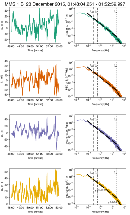
Figure 1: Time series of the magnetic field (GSE) components $\mathbb{B}=(B_{x},B_{y},B_{z})$ and the total magnitude $B_{T}=|\mathbb{B}|$ of the MMS data with the the corresponding spectrum of the high-resolution turbulence in the magnetosheath near the bow shock (BS), for frequencies above the ion gyrofrequency $f_{ci}$ marked by the dashed vertical line, and between the ion $f_{\lambda i}$ and above the electron $f_{\lambda e}$ Taylor-shifted inertial frequencies shown by the dashed–dotted and dotted lines, respectively (case (a) in Table 1 of Ref. Macek et al. 2018).

Figure 1 shows time series of all components of the magnetic field $\mathbb{B}=(B_{x},B_{y},B_{z})$ with its magnitude $B_{T}=|\mathbb{B}|$ in the GSM coordinates acquired by the MMS on 28 December 2015 during 5-minute time BURST interval (from 01.48:04 to 01.52:59), specified as case (a) in Table 1 of Ref. (Macek et al., 2018) with the corresponding Power Spectral Densities (PSD) of all the components of the magnetic field $\mathbf{B}$ obtained with the Welch’s (1967) windows. It is worth noting that for the magnetic spectrum above $f_{\lambda e}$ we enter the kinetic regime with the much steeper slope of -5.6 $\pm$ 0.3 that is consistent with the value of -16/3 predicted by kinetic theory of Alfvén waves (e.g., Schekochihin et al., 2009).

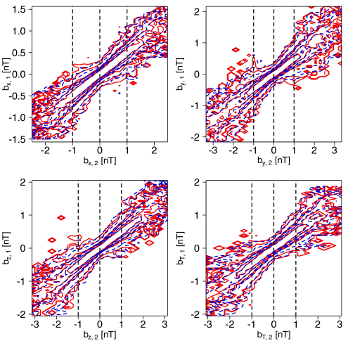
Figure 2: Comparison of the observed (red curves) contours plots of conditional probabilities at various scales $\tau$ reconstructed from the MMS magnetic field components in the magnetosheath, corresponding to spectra in Figure 1, with those reconstructed (dashed blue) according to the Chapman-Kolmogorov condition, Equation (3).

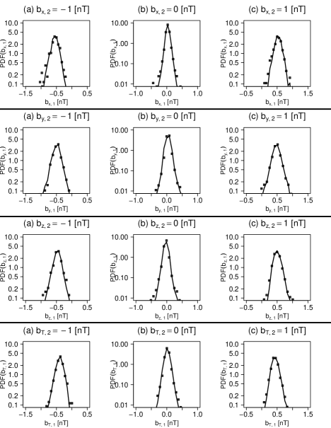
Figure 3: Comparison of cuts through $P(\mathbb{b}_{1},\tau_{1}|\mathbb{b}_{2},\tau_{2}$) for the fixed value of all components of the magnetic field increments $\mathbb{b}_{2}$ with $\tau_{1}$ = 0.02 s, $\tau^{\prime}$ = 0.0278 s, and $\tau_{2}$ = 0.0356 s.

First, according to Equation (1), we analyze increments of fluctuations $\mathbb{b}_{\tau}:=\mathbb{B}(t+\tau)-\mathbb{B}(t)$ across a time scale $\tau$ for each GSM component $x,y,z$ and the total intensity of the magnetic field $\mathbb{B}$. Using the conditional probability introduced in Section 3, we can compute $P(\mathbb{b}_{1},\tau_{1}|\mathbb{b}_{2},\tau_{2})$ on the right hand side of Equation (2) directly from the MMS data. Then, to verify a local transfer mechanism in the turbulence cascade, we can test whether the Chapman-Kolmogorov condition of Equation (3) is satisfied for the range of scales from $\tau_{1}$ to $\tau_{2}$, and $\tau_{1}<\tau’<\tau_{2}$.

In Figure 2 we compare the observed contour plots (red curves) of conditional probabilities at various scales $\tau$ with solutions (dashed blue) of Equation (3). The subsequent isolines correspond to the following decreasing levels of the conditional probability density function (from middle of the plots) for $\mathbb{b}$: 2, 1.1, 0.5, 0.3, 0.05, 0.02. In the corresponding Figure 3 we verify the Chapman-Kolmogorov equation (3) by comparison of cuts through the conditional probability distributions for some chosen values of parameter $\mathbb{b}$ in time series specified by Equation (1), which have been differentiated and the variance stationarity has been confirmed by using statistical augmented Dickey - Fuller test (Dickey & Fuller, 1979). We have chosen here for the magnetic field $\mathbb{b}_{\tau}$: $\tau_{1}$ = 0.02 s, $\tau^{\prime}$ = $\tau_{1}+\Delta t_{B}$ = 0.0278 s, and $\tau_{2}$ = $\tau_{1}+2\Delta t_{B}$ = 0.0356 s. We see that the Equation (3) is approximately satisfied up to the scales of about 100 $\Delta t_{B}$ = 0.78 s for $\mathbb{b}_{\tau}$ which indicates that the turbulence cascade exhibits Markov properties.

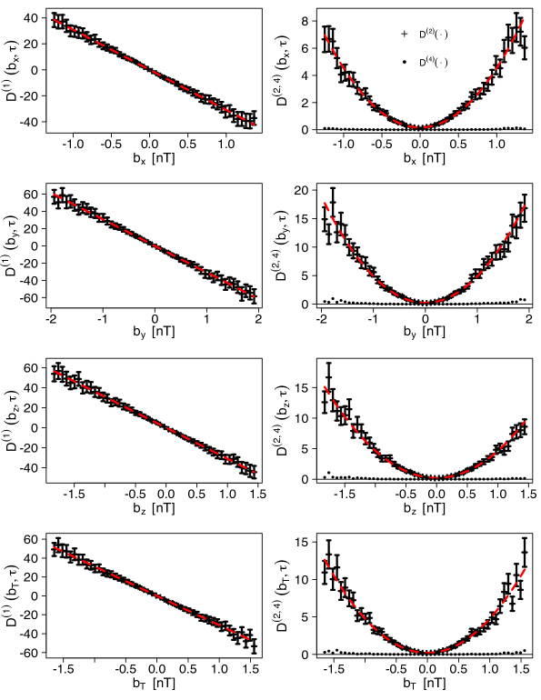
Figure 4: First and second finite-size Kramers-Moyal coefficients depending on the magnetic field increments $\mathbb{b}_{\tau}$ for all components of the magnetic field $\mathbf{B}=(B_{x},B_{y},B_{z})$ and the total magnitude $B_{T}=|\mathbb{B}|$. The dashed red lines show the best fits to the calculated values of $D^{(1)}(\mathbb{b},\tau)$ and $D^{(2)}(\mathbb{b},\tau)$ with $D^{(4)}(\mathbb{b},\tau)$ = 0, according to the Pawula’s theorem.

Second, we need to compute the Kramers-Moyal coefficients $D^{(k)}(x,\tau)$ in the Fokker-Planck expansion given by Equation (4). The values of the moments $M^{(k)}(x,\tau,\tau^{\prime})$ defined in Equation (5) can be obtained from the experimental data by counting the number $N(x^{\prime},x)$ of occurrences of fluctuations $x^{\prime}$ and $x$. Since the errors of $N(x^{\prime},x)$ are given by $1/\sqrt{N(x^{\prime},x)}$ the errors for the conditional moments $M^{(k)}(x,\tau,\tau^{\prime})$ can also be provided (see, Renner et al., 2001).

Admittedly $D^{(k)}(x,\tau)$ can only be obtained by extrapolation (for instance using piecewise linear regression) in the limit $\tau\rightarrow\tau^{\prime}$ in Equation (6), but we have checked that the very similar values are obtained taking the lowest time resolution $\tau-\tau^{\prime}=\Delta t_{B}$ = 0.0078 s. In fact, we have $D^{(k)}(x,\tau)\approx\frac{1}{k!}\frac{1}{\Delta t}M^{(k)}(x,\tau,\tau^{\prime})$. Therefore, basically the coefficients $D^{(k)}(x,\tau)$ show the same dependence on $x$ as $M^{(k)}(x,\tau,\tau‘)$ (cf. Renner et al., 2001). Figure 4 presents the fits to the first order drift $D^{(1)}(x,\tau)$ and the second order finite-size diffusion $D^{(2)}(x,\tau)$ coefficients for $\Delta t_{B}$ = 0.0078 s. We have also verified that the fourth-order coefficient $D^{(4)}(x,\tau)$ is close to zero for magnetic field data according to the Pawula’s theorem, which is a necessary and sufficient condition that the Kramers-Moyal expansion of Equation (4) stops after the second term.

In this case, we see that the best obtained fits to these lowest order coefficients are linear

$$D^{(1)}(x,\tau)=-a_{1}(\tau)x$$ (11)

and quadratic functions of $x$

$$D^{(2)}(x,\tau)=a_{2}(\tau)+b_{2}(\tau)x^{2},$$ (12)

respectively, where the appropriate fitted parameters $a_{k}$ for $k$ = 1 and 2 and $b_{2}$ depend on the time scale $\tau$. This corresponds to the generalized Ornstein-Uhlenbeck process. It is interesting to note that, similarly as obtained for the PSP data by Benella et al. (2022), who have looked at larger $\tau$, the best fit for any $x$ representing each component of $\mathbb{b}_{\tau}$ satisfies a power-law dependence $A\tau^{\alpha}$ with sufficient accuracy and the values for all the parameters are listed in Table 1.

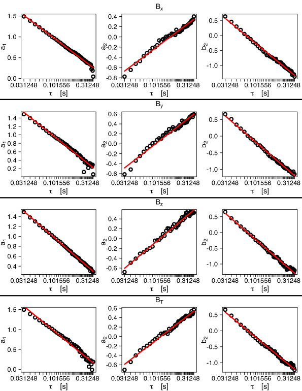
Figure 5: Linear dependence of the parameters $a_{1}$, $a_{2}$, and $b_{2}$ on logarithmic scale $\tau$, see Equations (11) and (12), for all components of the magnetic field $\mathbf{B}=(B_{x},B_{y},B_{z})$ and the total magnitude $B_{T}=|\mathbb{B}|$

Table 1: Parameters for Power-law Dependence of First and Second Kramers-Moyal Coefficients corresponding to Equations (11) and (12) for all components of the magnetic field $\mathbf{B}$ and the total magnitude $B_{T}=|\mathbb{B}|$

$b_{x}$	$A$	$\alpha$
$a_{1}$	0.6638 $\pm$ 0.0355	-1.2376 $\pm$ 0.0215
$a_{2}$	-0.4925 $\pm$ 0.0155	0.9416 $\pm$ 0.0094
$b_{2}$	0.5918 $\pm$ 0.0296	-1.6919 $\pm$ 0.0179

$b_{y}$	$A$	$\alpha$
$a_{1}$	0.6534 $\pm$ 0.0278	-1.2026 $\pm$ 0.0169
$a_{2}$	-0.4216 $\pm$ 0.0203	0.9699 $\pm$ 0.0123
$b_{2}$	0.5612 $\pm$ 0.0316	-1.5263 $\pm$ 0.0192

$b_{z}$ $A$ $\alpha$ $a_{1}$ 0.5646 $\pm$ 0.0286 -1.2253 $\pm$ 0.0173 $a_{2}$ -0.4024 $\pm$ 0.0172 1.0934 $\pm$ 0.0104 $b_{2}$ 0.5941 $\pm$ 0.0241 -1.6623 $\pm$ 0.0146 $b_{T}$ $A$ $\alpha$ $a_{1}$ 0.6989 $\pm$ 0.0225 -1.1191 $\pm$ 0.0089 $a_{2}$ -0.4946 $\pm$ 0.1259 1.1631 $\pm$ 0.0498 $b_{2}$ 0.5854 $\pm$ 0.0706 -1.7325 $\pm$ 0.0279

In fact, as seen in Figure 5 on logarithmic scale (cf. Strumik & Macek, 2008a, Fig. 5), we have verified here that for the MMS magnetic field data these lowest-order fits with power-law dependence apply for $\tau\leq 100\Delta t_{B}=\ 0.78$ s, when the probability density function is closer to Gaussian, $\tau\sim\tau_{G}$. However, for higher scales more complex functional dependence is necessary, especially in the inertial regime (Renner et al., 2001; Strumik & Macek, 2008a, b)

Anyway, we see again that using the simple linear and parabolic fits of Equations (11) and (12), the stationary solutions of Equation (10) become the well-known continuous kappa distributions (also known as Pearson type VII distribution), which probability density function is defined as:

$$p_{s}(x)=\frac{N_{o}}{\Big{[}1+\frac{1}{\kappa}\Big{(}\frac{x}{x_{o}}\Big{)}^{2}\Big{]}^{\kappa}}\ =\frac{N^{\prime}_{o}}{\Big{[}a_{2}(\tau)+b_{2}(\tau)x^{2}\Big{]}^{1+\frac{a_{1}(\tau)}{2b_{2}(\tau)}}}$$ (13)

with $\kappa=1+a_{1}(\tau)/[2b_{2}(\tau)]$ and $x_{o}^{2}=a_{2}(\tau)/b_{2}(\tau)/\kappa=a_{2}(\tau)/[b_{2}(\tau)+a_{1}(\tau)/2]$ (for $a_{2}(\tau)\neq 0$, $x_{o}(\tau)\neq 0$) and $N_{o}=p_{s}(0)$ satisfying the normalization $\int_{-\infty}^{+\infty}p_{s}(x^{\prime})dx^{\prime}=1$, i.e., $N_{o}=\frac{\Gamma(\kappa)}{x_{o}\sqrt{\pi\kappa}\Gamma(\kappa-1/2)}$. As requested, the boundary condition $p_{S}(x\rightarrow\pm\infty)\rightarrow 0$ is also verified here, and with $\kappa\rightarrow\infty$ the distribution degenerates into the Maxwellian distribution $N_{o}\mathrm{e}^{-(\frac{x}{x_{o}})^{2}}$ with $N_{o}=\frac{1}{x_{o}\sqrt{\pi}}$. The values of the relevant parameters of Equation (13) obtained by fitting the MMS data the given distributions are: $\kappa$ = 11.85673, $x_{0}$ = 1.756009, $N^{\prime}_{0}$ = 0.4121234, for $B_{x}$; $\kappa$ = 10.09043, $x_{0}$ = 3.05319, $N^{\prime}_{0}$ = 0.2684886, for $B_{y}$; $\kappa$ = 11.04104, $x_{0}$ = 2.779299, $N^{\prime}_{0}$ = 0.2802258, for $B_{z}$; $\kappa$ = 12.88198, $x_{0}$ = 1.75533, $N^{\prime}_{0}$ = 0.4133008, for $B_{T}$. These values of $\kappa$ would correspond to the nonextensivity parameter of the generalized (Tsallis’) entropy $q=1-1/\kappa\approx 0.9$, which is somewhat larger than $q\sim 0.5$ for $\kappa\sim 2$ reported for the PSP data by Benella et al. (2022).

In addition, substituting Equations (11) and (12) into Equation (7) we obtain

$$[a_{2}(\tau)+b_{2}(\tau)x^{2}]\frac{\partial^{2}P(x,\tau)}{\partial x^{2}}+[a_{1}(\tau)+4b_{2}(\tau)]x\frac{\partial P(x,\tau)}{\partial x}+\frac{\partial P(x,\tau)}{\partial\tau}+[a_{1}(\tau)+2b_{2}(\tau)]P(x,\tau)=0.$$ (14)

This means that in the Fokker-Planck Equations (9) and (14) become formally the second order parabolic partial differential equation.

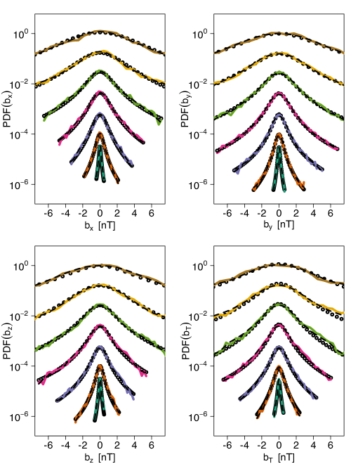
Figure 6: Comparison of the non-stationary (dashed lines) and the stationary (open points) solutions of the Fokker-Planck equation with the experimental probability density functions (PDF) of the magnetic field components $P(\mathbb{b},\tau)$ fluctuations (continuous colored lines) for all components of the magnetic field $\mathbf{B}=(B_{x},B_{y},B_{z})$ and the total magnitude $B_{T}=|\mathbb{B}|$ in the magnetosheath behind the bow shock using the MMS data, corresponding to spectra in Fig. 1, for various scales (shifted from bottom to top) $\tau$ = 0.0078, 0.04, 0.078, 0.12, 0.2, 0.39, and 0.78 s.

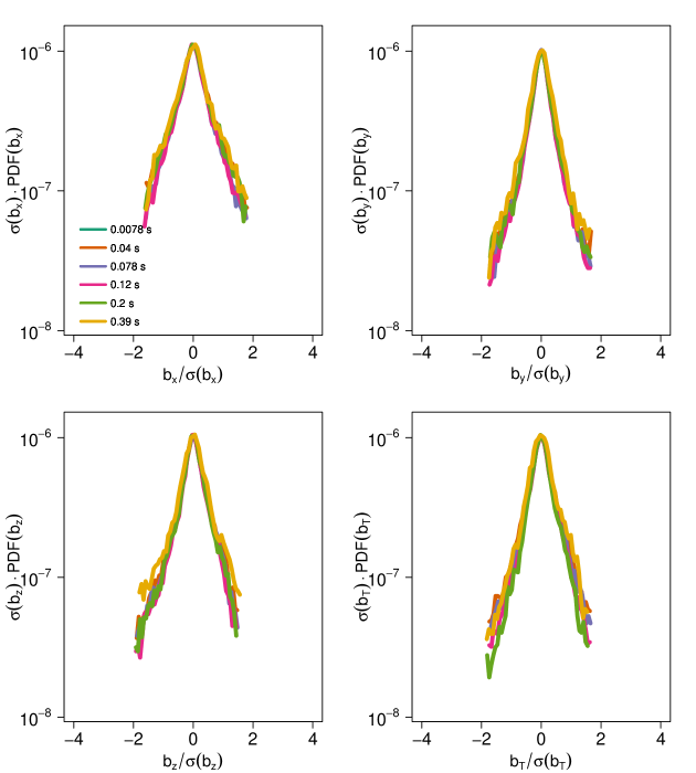
Figure 7: A universal scale invariance of the collapsing probability density functions of $\mathbb{b}_{\tau}$ rescaled by the respective standard deviations $\sigma_{\mathbb{b},\tau}$, corresponding to the kappa distributions in Figure 6 on the kinetic scales up to $\tau\sim 0.4$ s.

This in turn allows us to solve numerically non-stationary Fokker-Planck equation (dashed lines) using the numerical Euler integration scheme (verified for stationary solution $\frac{\partial P(x,\tau)}{\partial\tau}=0$, open points), which agrees with those obtained with modeling package by Rinn et al. (2016). We compare all these theoretical solutions with the probability density functions obtained directly from experimental data denoted by different colored continuous lines. This comparison is depicted in Figure 6 for various scales $\tau$, not greater than $\tau_{G}$, namely (from bottom to top) for $\tau$ = 1, 5, 10, 15, 25, 50, and 100 $\Delta t_{B}$ shifted in the vertical direction for clarity of presentation. For moderate values up to $\tau\sim 50\Delta t_{B}$ = 0.39 s in the case of linear and parabolic fits to Equations (11) and (12), we have the kappa distributions. However if we move to the larger scales $\tau_{G}$ from 100 $\Delta t_{B}$ = 0.78 s, the Kramers-Moyal coefficients $D^{(1)}$ and $D^{(2)}$ in Equation (4) are possibly described by more complex polynomial functions, but the probability density function is approximately Gaussian, as is expected for large values of $\kappa$. On the other hand, for the smallest available scales we see a very peaked density function (with large kurtosis), well described by the approximate shape of the Dirac delta function (formally in the limit of $\tau\rightarrow 0$).

In Figure 7, we have finally reproduced probability density functions of all components $\mathbb{b}_{\tau}$ rescaled by the respective standard deviations $\sigma_{\mathbb{b},\tau}$, which are consistent with the stationary solutions (open points) in Figure 6. Owing to a power-law dependence of the the first and second Kramers-Moyal parametrisation, as for PSP analysis by Benella et al. (2022), near the Sun with $\kappa\sim 2$ for scales up to $\tau\sim 0.05$ s, MMS data exhibit a universal global scale invariance mainly at 1 AU up to $\tau\sim 50\Delta t_{B}\sim 0.4$ s, where we have clear kappa distributions, but with some larger values of $\kappa\sim 10$. Since for somewhat larger scales from $\tau_{G}\sim 100\Delta t_{B}\sim 0.8$ s (not shown here) the respective kappa distributions are very close to a limiting Gaussian shape, this would result in some more deviations from the global scale invariance (not only on tails).

Our results demonstrate that the energy transfer among the different scales is essentially a stochastic process that can be modelled by the Fokker-Planck advection-diffusion equation also in the kinetic regime. As we already suggested in our earlier analysis for inertial range of scales (Strumik & Macek, 2008a, b), because the transfer among the different scales is a stochastic ‘memoryless’ process, we should expect a universal structure in the turbulent dynamics. This is actually shown by our statistical analysis of the probability density functions up to kinetic scales.

5 Conclusions

Magnetospheric Multiscale and Parker Solar Probe missions with unprecedented high millisecond time resolution of magnetometers data allow us to investigate turbulence on very small kinetic scales. In this paper we have looked at the MMS observations above 20 Hz, where the magnetic spectrum becomes very steep with the slope close to -16/3 resulting possibly from interaction between coherent structures.

Following our previous studies in the inertial region (Strumik & Macek, 2008a, b) we have shown for the first time that the Chapman-Kolmogorov equation, which is a necessary condition for Markovian character of turbulence, is satisfied exhibiting a local transfer mechanism of turbulence cascade also on much smaller kinetic scales. Moreover, we have verified that in this case the Fokker-Planck equation is reduced to drift and diffusion terms at least for scales smaller than 0.8 s.

In particular, similarly as for Parker Solar probe data analyzed by Benella et al. (2022) these lowest order coefficients are linear and quadratic functions of magnetic field, which correspond to the generalized Ornstein-Uhlenbeck processes. We have also recovered a similar universal scale invariance of the probability density functions up to kinetic scales of about 0.4 s.

It is interesting to note that for moderate scales we have also non-Gaussian (kappa) distribution, which for the smallest values of the available scale of 7.8 ms, is approximately described by a very peaked shape close to Dirac delta function. We also show that the normal Gaussian distribution is recovered for timescale two order larger (with large value of kappa parameter).

We hope that our observation of Markovian futures in solar wind turbulence could be important for understanding the relation between deterministic and stochastic properties of turbulence cascade at kinetic scales in complex astrophysical systems.

References

- Benella et al. (2022) Benella, S., Stumpo, M., Consolini, G., et al. 2022, The Astrophysical Journal Letters, 928, L21
- Biskamp (2003) Biskamp, D. 2003, Magnetohydrodynamic Turbulence (Cambridge, UK: Cambridge University Press)
- Bruno & Carbone (2016) Bruno, R., & Carbone, V. 2016, Lecture Notes in Physics, Vol. 928, Turbulence in the Solar Wind (Springer International Publishing, Berlin)
- Burch et al. (2016) Burch, J. L., Moore, T. E., Torbert, R. B., & Giles, B. L. 2016, Space Sci. Rev., 199, 5
- Chang (2015) Chang, T. T. S. 2015, An Introduction to Space Plasma Complexity (Cambridge University Press)
- Dickey & Fuller (1979) Dickey, D. A., & Fuller, W. A. 1979, Journal of the American Statistical Association, 74, 427
- Echim et al. (2021) Echim, M., Chang, T., Kovacs, P., et al. 2021, Turbulence and Complexity of Magnetospheric Plasmas (American Geophysical Union (AGU)), 67–91
- Frisch (1995) Frisch, U. 1995, Turbulence. The legacy of A.N. Kolmogorov (Cambridge: Cambridge University Press, —c1995)
- Macek et al. (2018) Macek, W. M., Krasińska, A., Silveira, M. V. D., et al. 2018, Astrophys. J. Lett., 864, L29
- Macek et al. (2019a) Macek, W. M., Silveira, M. V. D., Sibeck, D. G., Giles, B. L., & Burch, J. L. 2019a, Geophys. Res. Lett., 46
- Macek et al. (2019b) —. 2019b, Astrophys. J. Lett., 885, L26
- Macek et al. (2014) Macek, W. M., Wawrzaszek, A., & Burlaga, L. F. 2014, Astrophys. J. Lett., 793, L30
- Macek et al. (2011) Macek, W. M., Wawrzaszek, A., & Carbone, V. 2011, Geophys. Res. Lett., 38, L19103
- Macek et al. (2012) —. 2012, J. Geophys. Res., 117, 12101
- Macek et al. (2017) Macek, W. M., Wawrzaszek, A., Kucharuk, B., & Sibeck, D. G. 2017, Astrophys. J. Lett., 851, L42
- Macek et al. (2015) Macek, W. M., Wawrzaszek, A., & Sibeck, D. G. 2015, J. Geophys. Res., 120, 7466
- Papini et al. (2021) Papini, E., Cicone, A., Franci, L., et al. 2021, The Astrophysical Journal Letters, 917, L12
- Pedrizzetti & Novikov (1994) Pedrizzetti, G., & Novikov, E. A. 1994, Journal of Fluid Mechanics, 280, 69–93
- Renner et al. (2001) Renner, C., Peinke, J., & Friedrich, R. 2001, Journal of Fluid Mechanics, 433, 383–409
- Rinn et al. (2016) Rinn, P., Lind, P., Wächter, M., & Peinke, J. 2016, Journal of Open Research Software, 4, e34
- Risken (1996) Risken, H. 1996, The Fokker-Planck Equation: Methods of Solution and Applications, Springer Series in Synergetics (Springer Berlin Heidelberg)
- Russell et al. (2016) Russell, C. T., Anderson, B. J., Baumjohann, W., et al. 2016, Space Sci. Rev., 199, 189
- Schekochihin et al. (2009) Schekochihin, A. A., Cowley, S. C., Dorland, W., et al. 2009, ApJS, 182, 310
- Strumik & Macek (2008a) Strumik, M., & Macek, W. M. 2008a, Phys. Rev. E, 78, 026414
- Strumik & Macek (2008b) —. 2008b, Nonlinear Processes in Geophysics, 15, 607
- Wawrzaszek & Macek (2010) Wawrzaszek, A., & Macek, W. M. 2010, J. Geophys. Res., 115
- Welch (1967) Welch, P. D. 1967, IEEE Trans. Audio Electroacoust., 15, 70