Differentially Private Methods for Compositional Data

Abstract

Confidential data are increasingly common; some examples are electronic health records, activity data recorded from wearable devices, or geolocation. Differential privacy is a framework that enables statistical analyses while controlling the risk of leaking private information. Compositional data, which consists of vectors with positive components that add up to a constant, has received little attention in the differential privacy literature. In this article, we propose differentially private approaches for analyzing compositional data using the Dirichlet distribution. We consider several methods, including frequentist and Bayesian procedures.
Keywords: Data privacy, Bootstrap, Bayesian statistics, Dirichlet distribution

1 Introduction

A significant challenge in the statistical analysis of confidential data is the trade-off between obtaining accurate statistics and protecting sensitive information. To deal with this trade-off, differential privacy (DP), a definition proposed by Dwork et al. (2006), provides a formal framework that enables statistical analyses of confidential data while controlling the risk of leaking private information.

DP is a property held by randomized algorithms that are applied to confidential data sets. Most often, the outputs of DP methods are noisy versions of summary statistics. Under DP, users have access to those noisy summaries, but not to the confidential data set. Differentially private (DP) algorithms produce outputs that are robust to changes in an entry of the data set. As a result, the amount of information that attackers can learn about specific individuals is minimized.

A compositional datum is represented as a vector with positive components that add up to a constant which, without loss of generality, is assumed to be one. Compositional data arise in many disciplines. For example, sociologists measure time spent doing different daily activities; chemists study the composition of chemicals in samples; environmental scientists study material compositions in solid waste, and so on. Due to the widespread use of compositional data, considerable attention has been devoted to studying and developing methodologies for this type of data (Aitchison, 1982; Bacon-Shone, 2011; Ongaro and Migliorati, 2013). The Dirichlet distribution is a convenient model to analyze compositional data due to its mathematical properties and the ease of parameter interpretation.

In this work, we propose and evaluate DP approaches for analyzing compositional data using the Dirichlet distribution as the statistical model. We use DP to define a privatized summary statistic computed by adding random noise to a left-censored version of the sufficient statistic.

1.1 Related Work

Over the last few years, the development of approaches for making inferences under DP has received significant interest. Recent developments have focused on hypothesis testing for binomial data (Awan and Slavkovic, 2020), inference for linear regression models (Barrientos et al., 2019; Peña and Barrientos, 2021; Ferrando et al., 2022) , confidence intervals for the mean in normal models (Karwa and Vadhan, 2017), noise-aware Bayesian inference for linear regression (Bernstein and Sheldon, 2019) and generalized linear models (Kulkarni et al., 2021), among others. However, almost none of the existing methods can be applied to compositional data, which is the primary objective of this work. The technique proposed in Bernstein and Sheldon (2018), which applies to models within the exponential family, can be used for analyzing compositional data. However, it requires computing integrals that are not analytically available, and they are computationally expensive to evaluate via numerical methods. Another related article is Ferrando et al. (2022). Their work uses the parametric bootstrap to produce differentially private confidence intervals for distributions within the exponential family. In Ferrando et al. (2022), it is assumed that the support of the sufficient statistic is bounded. Unfortunately, this condition is not satisfied for the Dirichlet distribution.

1.2 Main contributions

Our contributions in this article can be summarized as follows:

• We propose frequentist and Bayesian methods for analyzing compositional data under differential privacy that are based on the Dirichlet distribution. Our methods rely on censored sufficient statistics.

• We study the effects of censoring the sufficient statistic. In addition, we propose a differentially private approach to select the censoring threshold.

• We discuss how to set prior distributions adequately. This is important because vague priors tend to perform poorly in this context.

• We describe algorithms for implementing the Bayesian approaches based on Markov Chain Monte Carlo, scalable strategies based on data-splitting, Approximate Bayesian Computation, and an asymptotic approximation proposed in Bernstein and Sheldon (2018).

• We make recommendations regarding which methods users can use depending on their modeling preferences and computational resources.

2 Background

This section describes the background required to develop the methods proposed in the article. The section begins with the definition of DP, its properties, and common strategies to achieve it. Then, we describe frequentist and Bayesian modeling strategies for compositional data based on the Dirichlet distribution.

2.1 Differential privacy

DP is a property of randomized algorithms (commonly known as mechanisms in the literature) used to generate noisy versions of summary statistics from a confidential data set.

Let $S$ be a random mechanism that takes as input a data set $\bm{D}=\{\bm{x}_{i}\}_{i=1}^{n}$, where $\bm{x}_{i}$ represents the $i$th individual in the sample. To define DP, we need to first define neighboring data sets. We say that $\bm{D}$ and $\bm{D}^{\prime}$ are neighbors if they are of the same size and differ only in one observation. Intuitively, DP ensures the outputs or summaries $S(\bm{D})$ and $S(\bm{D}^{\prime})$ are similar, implying that attackers cannot distinguish if a given output was computed based on $\bm{D}$ or $\bm{D}^{\prime}$. The similarity between $S(\bm{D})$ and $S(\bm{D}^{\prime})$ guarantees that very little information can be learned about what makes $\bm{D}$ and $\bm{D}^{\prime}$ different. Under DP, the “similarity” is controlled by a parameter commonly denoted by $\epsilon$ and referred to as the privacy budget. The privacy budget $\epsilon$ controls the degree of privacy offered by $S$, with lower values implying higher privacy levels. We now provide the formal definition of DP.

Definition 1.

Differential Privacy. Given $\epsilon>0$, a random mechanism $S$ is $\epsilon$-DP if for all pairs of neighboring data sets $(\bm{D},\bm{D}^{\prime})$, and for every $A\subseteq{\rm Range}(S)$, ${\rm Pr}\left[S(\bm{D})\in A|\bm{D}\right]\leq\exp(\epsilon){\rm Pr}\left[S(\bm{D}^{\prime})\in A|\bm{D}^{\prime}\right].$

In Definition 1, the data sets $(\bm{D},\bm{D}^{\prime})$ are treated as non-random objects. As $\epsilon$ decreases, the probability distributions of $S(\bm{D})$ and $S(\bm{D}^{\prime})$ become more similar (i.e., the privacy level increases). DP has several properties that make it particularly useful when designing statistical methods. Three relevant properties are post-processing, sequential composition, and parallel composition.

Proposition 1.

Post-processing. Given $S$ that satisfies $\epsilon$-DP and for any function $T$ defined on ${\rm Range}(S)$, the composition $T(S(\cdot))$ satisfies $\epsilon$-DP.

Proposition 2.

Sequential composition. Let $S_{1}$ and $S_{2}$ be $\epsilon_{1}$- and $\epsilon_{2}$-DP mechanisms, respectively. Then, the random mechanism $(S_{1}(\bm{D}),\,S_{2}(S_{1}(\bm{D}),\bm{D}))$ satisfies $(\epsilon_{1}+\epsilon_{2})$-DP.

Proposition 3.

Parallel composition. Let $S_{1},\,...\,,S_{K}$ be $K$ mechanisms that satisfy $\epsilon_{1}$-DP, $\cdots$, $\epsilon_{K}$-DP, respectively. Then, the joint mechanism $(S_{1}(\bm{D}_{1}),\,...\,,\,S_{K}(\bm{D}_{K}))$, where $\bm{D}_{1}\cap\cdots\cap\bm{D}_{K}=\varnothing$ and $\bm{D}_{1}\cup\bm{D}_{2}\cup\,...\,\cup\bm{D}_{k}\subset\bm{D}$ for $k\in\{1,\,...\,,K\}$, satisfies $\max_{k\in\{1,\cdots,K\}}\epsilon_{k}$-DP.

Proposition 1 implies that transforming the output of an $\epsilon$-DP mechanism does not incur on extra loss of privacy. Sequential composition (see Proposition 2) is a key property that indicates how to quantify the total privacy cost when multiple queries on $\bm{D}$ are requested. Parallel composition, described in Proposition 3, enables the modular design of mechanisms: if all the components of a mechanism are differentially private on disjoint data sets, then so is their composition with total privacy cost upper bounded by $\max_{k\in\{1,2,\cdots,K\}}\epsilon_{k}$. This property is guaranteed because we define neighboring data sets by replacing single observations, which leads to a specific notion of privacy known as bounded DP (Kifer and Machanavajjhala, 2011; Li et al., 2016).

Two privacy-ensuring mechanisms are relevant for this work: the Laplace and the Geometric mechanism. To define them, we first need to assume that our goal is to design a DP version of a summary statistic denoted by $S_{0}$. Then, we need to compute the global sensitivity of $S_{0}$, which is an upper bound on the maximum change (over all possible $\bm{D}$) that $S_{0}(\bm{D})$ can experience when a single observation is added or removed from $\bm{D}$.

Definition 2.

Global Sensitivity. The global sensitivity of the summary $S_{0}$, denoted by ${\rm GS}(S_{0})$, is defined as ${\rm GS}(S_{0})=\sup_{(\bm{D},\bm{D}^{\prime})}\lVert S_{0}(\bm{D})-S_{0}(\bm{D}^{\prime})\rVert_{1}$, where $\bm{D}$ and $\bm{D}^{\prime}$ are neighboring data sets.

The Laplace mechanism, proposed by Dwork et al. (2006), defines an $\epsilon$-DP version of $S_{0}$ by adding a Laplace-distributed perturbation term to $S_{0}(\bm{D})$. Specifically, for a real-valued function $S_{0}:\bm{D}\to\mathbb{R}^{d}$ with global sensitivity ${\rm GS}(S_{0})$ and privacy budget $\epsilon$, the output of the mechanism is $S_{L}(\bm{D}):=S_{0}(\bm{D})+\bm{\varepsilon}^{L}$, where $\bm{\varepsilon}^{L}$ is a $d$-dimensional vector with entries independently sampled from ${\rm Laplace}(0,{\rm GS}(S_{0})/\epsilon)$. The ${\rm Laplace}(m,s)$ distribution is parameterized by $(m,s)\in\mathbb{R}\times\mathbb{R}^{+}$ and its probability density function is $p_{\rm Lap}(\varepsilon^{L}\,|\,m,s)=\exp\left(-{|\varepsilon^{L}-m|}/{s}\right)/{2s},$ for $\varepsilon^{L}\in\mathbb{R}$.

The Geometric mechanism, proposed by Ghosh et al. (2012), is a discretized version of the Laplace mechanism. The Geometric mechanism adds random noise drawn from the two-sided geometric distribution, also known as the discrete Laplace distribution (Inusah and Kozubowski, 2006), to a discrete summary statistic. Specifically, for an integer-valued function $S_{0}:\bm{D}\to\mathbb{Z}^{d}$ with global sensitivity $GS(S_{0})$ and privacy budget $\epsilon$, the mechanism outputs $S_{G}(\bm{D}):=S_{0}(\bm{D})+\bm{\varepsilon}^{G}$, where $\bm{\varepsilon}^{G}$ is a $d$-dimensional vector with entries independently sampled from ${\rm TwoSidedGeometric}(\exp(-\epsilon/{\rm GS}(S_{0})))$. The probability mass function of the ${\rm TwoSidedGeometric}(t)$ distribution with parameter $t\in(0,1)$ is $p_{\rm TwoGeo}(\varepsilon^{G}\,|\,t)=t^{|\varepsilon^{G}|}\,(1-t)/(1+t),$ for $\varepsilon^{G}\in\mathbb{Z}$.

2.2 Compositional data and the Dirichlet distribution

In this section, we review facts about the Dirichlet distribution that are useful for our purposes. We begin by setting our notation. Assume that we have information on $n$ individuals where each observation is compositional. That is, for each individual $i\in\{1,\dots,n\}$, the corresponding compositional observation $\bm{x}_{i}=(x_{i1},\dots,x_{id})^{T}$ is a vector taking values on the $(d-1)$-dimensional simplex $\Delta_{d-1}=\left\{(x_{1},\,...\,,x_{d})^{T}:x_{j}\geq 0,\sum_{j=1}^{d}x_{j}=1\right\}.$ From now on, we denote the compositional data set by $\bm{D}=[\bm{x}_{1},\,...\,,\bm{x}_{n}]^{T}$.

To model $\bm{D}$, we assume that $\bm{x}_{1},\dots,\bm{x}_{n}$ is a random sample from a Dirichlet distribution with parameter $\bm{\alpha}=(\alpha_{1},\dots,\alpha_{d})^{T}$, which we denote by $\bm{x}_{i}\,|\,\bm{\alpha}\overset{\rm iid}{\sim}{\rm Dirichlet}(\bm{\alpha}).$ It is straightforward to see that the Dirichlet distribution is a member of the exponential family and that $S_{0}(\bm{D})=n^{-1}\left(\sum_{i=1}^{n}\log x_{i1},\,...\,,\sum_{i=1}^{n}\log x_{id}\right)^{T}$ is a sufficient statistic.

We consider frequentist and Bayesian approaches to make inferences about $\bm{\alpha}$. In both paradigms, the sufficient statistic $S_{0}(\bm{D})$ is enough to perform full inference and prediction.

For frequentist inference, we focus on the maximum likelihood estimator (MLE) of $\bm{\alpha}$. Given that the MLE cannot be computed analytically, Minka (2000) proposed a convergent fixed point iteration algorithm for estimating $\bm{\alpha}$.

Bayesian inference requires specifying a prior probability distribution on $\bm{\alpha}$ that represents the available prior information about this parameter. Since $\bm{\alpha}$ takes values on $\mathbb{R}^{d}_{+}$, the prior distribution, denoted as $\pi_{0}$, also has to be defined on $\mathbb{R}^{d}_{+}$. The posterior distribution of $\bm{\alpha}$ is given by

$$\pi(\bm{\alpha}\,|\,S_{0}(\bm{D})) \propto e^{(\bm{\alpha}-\bm{1})^{T}nS_{0}(\bm{D})-C(\bm{\alpha})}\prod_{j=1}^{d}\pi_{0}(\bm{\alpha}),\,\,\,\bm{\alpha}\in\mathbb{R}^{d}_{+},$$ (1)

where $\bm{1}$ is a column vector with $d$ ones and $C(\bm{\alpha})$ is the cumulant function.

3 Differentially Private Methods

In this section, we define and study the properties of the methods we propose in this article. When the data are not confidential, it suffices to have access to $S_{0}(\bm{D})$ to make inferences about the unknown parameter $\bm{\alpha}$. However, direct access to summaries such as $S_{0}(\bm{D})$ may result in leakage of private information, as discussed in Section 2.1.

In Section 3.1, we describe a strategy to define a DP version of $S_{0}(\bm{D})$. In Section 3.2, we introduce a frequentist approach based on the MLE of $\bm{\alpha}$ and the parametric bootstrap. In Section 3.3, we describe multiple Bayesian approaches that combine different prior distributions and computational strategies such as MCMC algorithms, ABC techniques, and asymptotic approximations.

3.1 Differentially private sufficient statistic

To create a DP version of $S_{0}(\bm{D})$, one cannot apply the Laplace mechanism directly because its is unbounded: the entries of a compositional datum can be arbitrarily close to zero, so the logarithm can diverge to $-\infty$.

To bound the global sensitivity of $S_{0}$, we propose left-censoring the observations at a small value $a\in(0,1)$, defining $\tilde{\bm{x}}_{i}=(\max\{x_{i1},a\},\,...\,,\max\{x_{id},a\})$ and $\tilde{\bm{D}}=[\tilde{\bm{x}}_{1},\dots,\tilde{\bm{x}}_{n}^{*}]^{T}$. After applying the left-censoring to the observations, the global sensitivity becomes ${\rm GS}(S_{0})=n^{-1}\sup_{\bm{x},\bm{x}^{\prime}\in\Delta_{d-1}}\|(\tilde{x}_{1}-\tilde{x}_{1}^{\prime},\,...\,,\tilde{x}_{d}-\tilde{x}_{d}^{\prime})\|_{1}\leq-2n^{-1}d\log a$. To make explicit the dependence on $a$, we denote the censored sufficient statistic as $S_{0}(\bm{D},a)$.

After defining $S_{0}(\bm{D},a)$, we can apply the Laplace mechanism. We define $S_{L}(\bm{D},a):=S_{0}(\bm{D},a)+\bm{\varepsilon}^{L}$, where the entries of $\bm{\varepsilon}^{L}$ are independently sampled from ${\rm Laplace}(0,-d\log a/(n\epsilon_{1}))$. The statistic $S_{L}(\bm{D},a)$ is an $\epsilon_{1}$-DP version of $S_{0}(\bm{D},a)$, and our goal is making inferences about $\bm{\alpha}$ based on $S_{L}(\bm{D},a)$. Clearly, $S_{L}(\bm{D},a)$ converges in probability to $S_{0}(\bm{D},a)$ as the sample size $n$ increases for a fixed privacy budget $\varepsilon_{1}$.

3.1.1 Effects of censoring the sufficient statistic

In this section, we study the effects of censoring the sufficient statistic. We do so by finding the expected proportion of entries that are censored and the bias induced by censoring. From our analysis, we conclude that inferences based on the censored data will be close to what we would obtain without censoring if $a$ is small (relative to the expected value of $x_{ij}$) and $\sum_{k=1}^{d}\alpha_{k}$ is not near zero.

The probability that each entry $x_{ij}$ is censored is $P(x_{ij}<a)=P(\mathrm{Beta}(\alpha_{j},\beta_{j})<a)=I_{a}(\alpha_{j},\beta_{j}),$ where $I_{a}(\cdot,\cdot)$ is the incomplete beta function and $\beta_{j}=\sum_{k=1}^{d}\alpha_{k}-\alpha_{j}$. The higher $a$ is, the more likely it is that an entry will be censored.

A quantity that summarizes the extent to which there are censored entries in our data set is the expected proportion of censored entries $x_{ij}$:

$$E\left[\frac{1}{{nd}}\sum_{i=1}^{n}\sum_{j=1}^{d}\mathbbm{1}(x_{ij}<a)\right]=\frac{1}{nd}\sum_{i=1}^{n}\sum_{j=1}^{d}P(x_{ij}<a)=\frac{1}{d}\sum_{j=1}^{d}P(x_{ij}<a).$$

Figure 1(a) shows the expected proportion of censored entries as a function of $a$ for three different values of $\bm{\alpha}$. Unsurprisingly, the expected proportion increases in $a$. More interestingly, we observe that, as $\sum_{k=1}\alpha_{k}$ grows, the expected proportion is low for small values of $a$, but then increases more rapidly as $a$ increases.

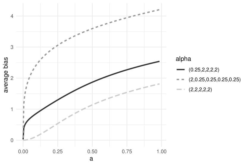
(a)

(b)

Figure 1: (a) Proportion of censored entries as a function of $\bm{\alpha}$ and $a$ (b) Average bias of censored DP statistic as a function of $\bm{\alpha}$ and $a$.

From an analytical point of view, we can bound the beta CDF with a Bernstein-type bound derived in Skorski (2023). First of all, define

$$m_{j}=\frac{\alpha_{j}}{\sum_{k=1}^{d}\alpha_{k}},\,\,v_{j}=\frac{\alpha_{j}\beta_{j}}{(\sum_{k=1}^{d}\alpha_{k})^{2}(\sum_{k=1}^{d}\alpha_{k}+1)},\,\,c_{j}=\frac{2(\sum_{k=1}^{d}\alpha_{k}-2\alpha_{j})}{\sum_{k=1}^{d}\alpha_{k}(\sum_{k=1}^{d}\alpha_{k}+2)}.$$

Then, the probability that $x_{ij}$ is censored can be bounded as follows:

$$P(x_{ij}<a)\leq\begin{cases}e^{\frac{-(m_{j}-a)^{2}}{2[v_{j}+c_{j}(m_{j}-a)/3]}},&\text{ if }\alpha_{j}\geq\sum_{k=1}^{d}\alpha_{k}/2\\ e^{\frac{-(m_{j}-a)^{2}}{2v_{j}}},&\text{ if }\alpha_{j}<\sum_{k=1}^{d}\alpha_{k}/2.\end{cases}$$

Most commonly, $\alpha_{j}<\sum_{k=1}^{d}\alpha_{k}/2$, unless the $j$-th component of $\alpha$ dominates over the others. Both cases are exponentially decreasing in $E(x_{ij})-a$ provided that $E(x_{ij})>a$, which in practice almost always holds because $a$ is chosen to be small.

Another helpful metric for quantifying the effects of censoring is the bias of the censored statistic. To obtain that quantity, we need to find the expected values of $S_{0}(\bm{D},a)$ and $S_{L}(\bm{D},a)$. The expectation of $\bm{\varepsilon}^{L}$ is zero, so $E[S_{0}(\bm{D},a)]=E[S_{L}(\bm{D},a)]$. The expected value of $\log\tilde{x}_{ij}$ is

$$E[\log\tilde{x}_{ij}]=E(\log x_{ij})+P(x_{ij}<a)\log a-\mathcal{I}_{a},\,\,\,\,\mathcal{I}_{a}=\int_{0}^{a}\log x_{ij}\,\mathrm{Beta}(x_{ij}\,|\,,\alpha_{j},\beta_{j})\,\mathrm{d}x_{ij}.$$

The bias induced by censoring in the $j$-th component is

$$E[\log\tilde{x}_{ij}]-E[\log x_{ij}]=\int_{0}^{a}(\log a-\log x_{ij})\,\mathrm{Beta}(x_{ij}\,|\,\alpha_{j},\beta_{j})\,\mathrm{d}x_{ij}>0.$$

The bias is clearly increasing in $a$, as expected. In order to study the behavior of the bias analytically, we find an upper bound on the bias. Assuming $\alpha_{j}>1$, we can use the bound $\log x_{ij}>1-1/x_{ij}$ to do so:

$$E[\log\tilde{x}_{ij}]-E[\log x_{ij}] \leq\int_{0}^{a}(\log a+1/x_{ij}-1)\,\mathrm{Beta}(x_{ij}\,|\,,\alpha_{j},\beta_{j})\,\mathrm{d}x_{ij}$$

$$\leq\frac{B(\alpha_{j}-1,\beta_{j})}{B(\alpha_{j},\beta_{j})}P(\mathrm{Beta}(\alpha_{j}-1,\beta_{j})\leq a),$$

where $B(\cdot,\cdot)$ is the beta function. The ratio $B(\alpha_{j}-1,\beta_{j})/B(\alpha_{j},\beta_{j})$ decreases to 1 as $\sum_{k=1}^{d}\alpha_{k}$ increases, so the bound decreases as $\sum_{k=1}^{d}\alpha_{k}$ increases. The beta tail probability can be bounded using the Bernstein-type bound we used in the previous section, which exponentially decreases in $E(x_{ij})-a.$

Figure 1(b) shows the average bias across the $d$ components of $x_{i}$ as a function of $a$ for the same values of $\alpha$ we considered in Figure 1(a). Again, the bias is increasing in $a$. We also observe that the bias decreases in $\sum_{k=1}^{d}\alpha_{k}$, as we observed in the upper bound.

3.1.2 Selecting the threshold for censoring the sufficient statistic

Since $S_{L}(\bm{D},a)$ depends on $a$, we develop a DP algorithm to select it. There is a bias-variance trade-off in selecting $a$. Small values of $a$ imply $S_{0}(\bm{D},a)\approx S_{0}(\bm{D})$, but they lead to large variances in $\bm{\varepsilon}^{L}$. Conversely, large values of $a$ induce substantial bias, but lead to small variances in $\bm{\varepsilon}^{L}$.

We select $a$ from a list of $M$ candidates ${a_{1},\,...\,,a_{M}}$ where $a_{1}>\,...\,>a_{M}$. To define our strategy, we keep track of the number of uncensored individuals for each of the candidates, which we denote $u_{1},u_{2},\,...\,,u_{M}$. Since the candidates are arranged in decreasing order, we have that $u_{1}\leq u_{2}\leq\,...\,\leq u_{M}$.

To select $a$ among the candidates, we define $\mathrm{Score}(\bm{D})=(s_{1},s_{2},\,...\,,s_{M})$, where $s_{m}=u_{m}-u_{m-1}$ for $m\in\{1,\,...\,,M\}$ with $u_{0}=0$. While $s_{1}$ corresponds to the number of uncensored observations if $a=a_{1}$, $s_{m}$ counts the additional uncensored observations we obtain if we use $a_{m}$ instead of $a_{m-1}$. If $s_{m}=0$, then $a_{m-1}$ is clearly preferable to $a_{m}$. If it is non-zero, we need a criterion to decide if we move from $a_{m-1}$ to $a_{m}$ or not. The criterion we use is the following: use $a_{1}$ if $s_{1}>0.99n$; otherwise, do not move from $a_{m-1}$ to $a_{m}$ if $s_{m}<0.01n.$

Unfortunately, we cannot use $\mathrm{Score}(\bm{D})$ directly because it might leak private information, so we define a DP version of it. Given that $\mathrm{Score}(\bm{D})$ is discrete and ${\rm GS}(\mathrm{Score})=2$, we can use the Geometric mechanism to define $S_{G}(\bm{D})=(s_{G,1},\,...\,,s_{G,M})=\mathrm{Score}(\bm{D})+\bm{\varepsilon}^{G}$, where the entries of $\bm{\varepsilon}^{G}$ are independently sampled from ${\rm TwoSidedGeometric}(\exp(-\epsilon_{2}/2))$. To account for the noise added to the score function and ensure it is worth moving from $a_{m-1}$ to $a_{m}$ with low uncertainty, we find $95\%$ confidence intervals for $\mathrm{Score}(\bm{D})$ based on $S_{G}(\bm{D})$ and percentiles of $\varepsilon^{G}\sim{\rm TwoSidedGeometric}(\exp(-\epsilon_{2}/2))$. If $\varepsilon^{G}_{0.025}$ and $\varepsilon^{G}_{0.975}$ are the largest and smallest integers such that $P(\varepsilon^{G}\leq\varepsilon^{G}_{0.025})\leq 0.025$ and $P(\varepsilon^{G}\geq\varepsilon^{G}_{0.975})\geq 0.025$, we select $a$ with the function

$$A(S_{G}(\bm{D}))=\begin{cases}a_{1}&\text{if }s_{G,1}+\varepsilon^{G}_{0.975}\geq 0.99n\\ \max\mathcal{A}_{2:M}&\text{if }s_{G,1}+\varepsilon^{G}_{0.975}<0.99n\text{ and }\mathcal{A}_{2:M}\neq\emptyset\\ a_{M}&\text{otherwise}\end{cases}$$

where $\mathcal{A}_{2:M}=\left\{a_{m}:\,s_{G,m}-\varepsilon^{G}_{0.025}\geq 0.01n,\,m\in\{2,\,...\,,M\}\right\}$. If the interval for $s_{1}$ indicates it is above $0.99n$, then we set $a=a_{1}$. Otherwise, we select the smallest $a_{m}$ whose interval indicates that the corresponding $s_{m}$ is above $0.01n$. When the interval for $s_{1}$ is not above $0.99n$ and the one for $s_{m}$ is not above $0.01n$ for all $m$, we set $a=a_{1}$. This last scenario might happen, for example, if the $u_{m}$ are all the same and smaller than $0.99n$.

3.1.3 Releasing the differentially private statistic

In this section, we describe the algorithm we follow to release the differentially private statistic.

Algorithm 1 displays the steps that analysts must follow to release either $S_{L}(\bm{D},a)$ or $S_{L}(\bm{D}_{1},a)$ and $S_{L}(\bm{D}_{2},a)$. We conclude this section with a formal theorem that Algorithm 1 is $(\epsilon_{1}+\epsilon_{2})$-DP. The proof can be found in the Supplementary Material.

Theorem 1.

Algorithm 1 satisfies $(\epsilon_{1}+\epsilon_{2})$-DP.

Algorithm 1 $(\epsilon_{1}+\epsilon_{2})$-DP algorithm to select $a$ and release DP statistic

procedure DPss($\bm{D},\epsilon_{1},\epsilon_{2},(a_{1},a_{2},\,...\,,a_{M})$, $n_{1}$, $n_{2}$)

     draw $\varepsilon^{G}_{m}\overset{\mathrm{iid}}{\sim}{\rm TwoSidedGeometric}(\exp(-\epsilon_{2}/2))$, $m=1,\,...\,,M$

     compute $S_{G}(\bm{D})=(s_{G,1},\,...\,,s_{G,M})=\mathrm{Score}(\bm{D})+(\varepsilon^{G}_{1},\,...\,,\varepsilon^{G}_{M})$

     select $a$ using the function $A(S_{G}(\bm{D}))$

     if $n_{1}=0$ then

         draw $\varepsilon^{L}_{j}\overset{\mathrm{iid}}{\sim}{\rm Laplace}(0,-d\log(a)/(n\epsilon_{1}))$, $j\in\{1,\,...\,,d\}$

         compute $S_{L}(\bm{D},a)=S_{0}(\bm{D},a)+(\varepsilon^{L}_{1},\dots,\varepsilon^{L}_{d})$

         return $S_{G}(\bm{D})$, $a$, and $S_{L}(\bm{D},a)$

     else

          Split $\bm{D}$ uniformly at random into $\bm{D}_{1}$ and $\bm{D}_{2}$

         draw $\varepsilon^{L}_{j,l}\overset{\mathrm{iid}}{\sim}{\rm Laplace}(0,-d\log(a)/(n\epsilon_{1}))$, $j\in\{1,\,...\,,d\}$, $l\in\{1,2\}$

         compute $S_{L}(\bm{D}_{l},a)=S_{0}(\bm{D}_{l},a)+(\varepsilon^{L}_{1,l},\dots,\varepsilon^{L}_{d,l})$, $l\in\{1,2\}$

         return $S_{G}(\bm{D})$, $a$, $S_{L}(\bm{D}_{1},a)$, and $S_{L}(\bm{D}_{2},a)$      

3.2 Frequentist methods

As discussed in Section 2.2, we can obtain an MLE estimate of the parameter of interest $\bm{\alpha}$ using the sufficient statistic $S_{0}(\bm{D})=S_{0}(\bm{D},0)$ and the convergent fixed point iteration technique proposed by Minka (2000). Let ${\rm MLE}(S_{0}(\bm{D},0))$ be the function returning the MLE of $\bm{\alpha}$. Since $S_{L}(\bm{D},a)$ is assumed to be an approximation of $S_{0}(\bm{D},0)$, which is in turn an approximation of $S_{0}(\bm{D},a)$, with $a=A(S_{G}(\bm{D}))$, we could obtain a DP estimate of $\bm{\alpha}$ using ${\rm MLE}(S_{L}(\bm{D},a))$. However, to obtain proper inferences, we cannot omit the censoring and noise added when computing $S_{L}(\bm{D},a)$. To account for these aspects, we use the parametric bootstrap (Efron, 2012) to approximate the distribution of ${\rm MLE}(S_{L}(\bm{D},a))$.

To implement the parametric bootstrap, we first account for the noise added to $S_{0}(\bm{D},a)$ by subtracting $\bm{\varepsilon}^{L}$ from $S_{L}(\bm{D},a)$ and defining $\widetilde{S_{0}}(\bm{D},a)=S_{L}(\bm{D},a)-\bm{\varepsilon}^{L}$. Then, we compute $\bm{\alpha}^{*}={\rm MLE}(\widetilde{S_{0}}(\bm{D},a))$ and, to account for sampling error, generate a simulated data set $\widetilde{\bm{D}}$ of size $n$ using ${\rm Dirichlet}(\bm{\alpha}^{*})$. Finally, we compute $S_{0}(\widetilde{\bm{D}},a)$, which now accounts for the censoring, and obtain $\widetilde{\bm{\alpha}}={\rm MLE}(S_{0}(\widetilde{\bm{D}},a))$. We use the distribution of $\widetilde{\bm{\alpha}}$ to approximate the sampling distribution of ${\rm MLE}(S_{L}(\bm{D},a))$. Algorithm 2, henceforth DPBoots, summarizes our strategy.

Now, we justify why we propose Algorithm 2 as a parametric bootstrap algorithm. In the usual, non-private parametric bootstrap, we would sample from $p_{\rm Dir}(\bm{x};\,\bm{\alpha}={\rm MLE}(S_{0}(\bm{D})))$. If we observe $S_{L}(\bm{D})=S_{0}(\bm{D})+\bm{\varepsilon}^{L}$ instead, we can rewrite the parametric bootstrap conditional on $\bm{\varepsilon}^{L}$ as $p_{\rm Dir}(\bm{x};\,\bm{\alpha}={\rm MLE}(S_{L}(\bm{D})-\bm{\varepsilon}^{L})\,|\,\bm{\varepsilon}^{L}),$ where $S_{L}(\bm{D})-\bm{\varepsilon}^{L}$ must be in ${\rm Range}(S_{0})$. Here, we must assume that $S_{0}(\bm{D})\approx S_{0}(\bm{D},a)$, which is something we can verify using the DP score function $S_{G}(\bm{D})$. Evidence against such an assumption arises when the selected threshold is $a=a_{1}$ (the smallest one among the $M$ candidates), and $s_{G,1}$ (the noisy version of the number of individuals who do not need to be censored with $a=a_{1}$) is close to $n$. Thus, $S_{0}(\bm{D})\approx S_{0}(\bm{D},a)$ implies that $S_{L}(\bm{D})\approx S_{L}(\bm{D},a)=S_{0}(\bm{D},a)+\bm{\varepsilon}^{L}$ and $p_{\rm Dir}(\bm{x};\,\bm{\alpha}={\rm MLE}(S_{L}(\bm{D})-\bm{\varepsilon}^{L})\,|\,\bm{\varepsilon}^{L})\approx p_{\rm Dir}(\bm{x};\,\bm{\alpha}={\rm MLE}(S_{L}(\bm{D},a)-\bm{\varepsilon}^{L})\,|\,\bm{\varepsilon}^{L}).$

Since the distribution of $\bm{\varepsilon}^{L}$ is known, the bootstrap data-generating mechanism is the convolution

$$\int_{{\rm Range}({\rm Lap};\,S_{L}(\bm{D},a))}p_{\rm Dir}(\bm{x};\,\bm{\alpha}={\rm MLE}(S_{L}(\bm{D},a)-\bm{\varepsilon}^{L})\,|\,\bm{\varepsilon}^{L})\,p_{\rm Lap}(\bm{\varepsilon}^{L};S_{L}(\bm{D},a)\,\,|\,0,m)\,\mathrm{d}\bm{\varepsilon}^{L}.$$

where $m=-d\log(a)/(n\epsilon_{1})$

$${\rm Range}({\rm Lap};\,S_{L}(\bm{D},a)) =\{\bm{\varepsilon}:\,S_{L}(\bm{D},a)-\bm{\varepsilon}\in{\rm Range}(S_{0})\},$$

$${\rm Range}(S_{0}) =\left\{(s_{0,1},\,...\,,s_{0,d})\in(-\infty,0)^{d}\,:\,\sum_{j=1}^{d}\exp(s_{0,j})\leq 1\right\},$$

and

$$p_{{\rm Lap}}(\bm{\varepsilon}^{L};S_{L}(\bm{D},a)\,|0,m)=\frac{\prod_{j=1}^{d}p_{\rm Lap}(\varepsilon^{L}_{j}|0,m)\,\mathbbm{1}(\bm{\varepsilon}^{L}\in{\rm Range}({\rm Lap};\,S_{L}(\bm{D},a)))}{\int_{{\rm Range}({\rm Lap};\,S_{L}(\bm{D},a))}\prod_{j=1}^{d}p_{\rm Lap}(\varepsilon^{L}_{j}|0,m)\,\mathrm{d}\bm{\varepsilon}^{L}}.$$

In the convolution, we use the truncated Laplace distribution $p_{{\rm Lap}}(\bm{\varepsilon}^{L};S_{L}(\bm{D},a),|0,m)$. The reason is that $S_{L}(\bm{D},a)$ provides valuable information about the noise initially added to $S_{0}(\bm{D},a)$. This situation is analogous, for instance, to the case where the summary of interest is a count, and the observed noisy count is negative, which would inherently indicate that the added noise was not greater than zero.

Algorithm 2 DP parametric bootstrap to estimate $\bm{\alpha}$

procedure DPBoots ($S_{L}(\bm{D},a),\epsilon_{1},a,n$)

     repeat i) draw $\varepsilon^{L}_{j}\overset{\mathrm{iid}}{\sim}{\rm Laplace}(0,-d\log(a)/(n\epsilon_{1}))$, $j=1,\,...\,,d$ ii) compute $\widetilde{S_{0}}(\bm{D},a)={\color[rgb]{0,0,0}(\tilde{s}_{0,1},\,...\,,\tilde{s}_{0,d})}=S_{L}(\bm{D},a)-(\varepsilon^{L}_{1},\dots,\varepsilon^{L}_{d})$ if $\sum_{j=1}^{d}\exp(\tilde{s}_{0,j})\leq 1$, proceed to iii); otherwise, return to i) iii) compute $\bm{\alpha}^{*}={\rm MLE}(\widetilde{S_{0}}(\bm{D},a))$ iv) generate simulated data set $\widetilde{\bm{D}}$ of size $n$ from ${\rm Dirichlet}(\bm{\alpha}^{*})$ v) obtain estimate $\widetilde{\bm{\alpha}}={\rm MLE}(S_{0}(\widetilde{\bm{D}}))$

     until reach a desired number of iterations

return all $\widetilde{\bm{\alpha}}$’s obtained in all iterations

3.3 Bayesian methods

Under the Bayesian paradigm, inferences rely on the posterior distribution of $\bm{\alpha}$ conditional on the available information. Due to privacy constraints, we assume that the only available information is $S_{L}(\bm{D},a)$, the DP version of the sufficient statistic.

To use model (1), we need to treat either $\bm{D}$ or $S_{0}(\bm{D},a)$ as an unknown quantity and account for the noise added to it to define $S_{L}(\bm{D},a)$. As a result, an adequate inferential strategy must use the joint distribution of $(\bm{\alpha},S_{0}(\bm{D},a))$ or $(\bm{\alpha},\bm{D})$ conditional on $S_{L}(\bm{D},a)$, which is given by

$$\pi(\bm{\alpha},\bm{D}|S_{L}(\bm{D},a)=\bm{s}_{L})\propto$$

$$\prod_{j=1}^{d}p_{\rm Lap}\left(s_{0,j}\left|s_{L,j},-\frac{d\log(a)}{n\epsilon_{1}}\right.\right)p(\bm{D}|\bm{\alpha})\pi_{0}(\bm{\alpha}),$$ (2)

$$\pi(\bm{\alpha},S_{0}(\bm{D},a)|S_{L}(\bm{D},a)=\bm{s}_{L})\propto$$

$$\prod_{j=1}^{d}p_{\rm Lap}\left(s_{0,j}\left|s_{L,j},-\frac{d\log(a)}{n\epsilon_{1}}\right.\right)e^{(\bm{\alpha}-\bm{1})^{T}nS_{0}(\bm{D},a)-C(\bm{\alpha})}\pi_{0}(\bm{\alpha})$$ (3)

where $s_{0,j}$ and $s_{L,j}$ represent the $j$-th component of $S_{0}(\bm{D},a)$ and $\bm{s}_{L}$, respectively. Analysts will use $\pi(\bm{\alpha}|S_{L}(\bm{D},a)=\bm{s}_{L})$, which is obtained by integrating out $\bm{D}$ in (2) or $S_{0}(\bm{D},a)$ in (3).

We consider using a fraction of the data for prior elicitation. Specifically, we partition $\bm{D}$ into two disjoint subsets $\bm{D}_{1}$ and $\bm{D}_{2}$, and use $S_{L}(\bm{D}_{1},a)$ for prior elicitation and $S_{L}(\bm{D}_{2},a)$ to define the likelihood. Under this alternative strategy, we use the joint distribution

$$\pi(\bm{\alpha},S_{0}(\bm{D}_{2},a)|S_{L}(\bm{D}_{2},a)=\bm{s}_{L}^{(2)},S_{L}(\bm{D}_{1},a)=\bm{s}_{L}^{(1)})\propto$$

$$\prod_{j=1}^{d}p_{\rm Lap}\left(s_{0,j}^{(2)}\left|s_{L,j}^{(2)},\frac{-d\log(a)}{n_{2}\epsilon_{1}}\right.\right)e^{(\bm{\alpha}-\bm{1})^{T}n_{2}S_{0}(\bm{D}_{2},a)-C(\bm{\alpha})}\pi_{0}(\bm{\alpha}|S_{L}(\bm{D}_{1},a)=\bm{s}_{L}^{(1)})$$ (4)

where $s_{0,j}^{(2)}$, $s_{L,j}^{(2)}$, and $s_{L,j}^{(2)}$ represent the $j$-th component of $S_{0}(\bm{D}_{2},a)$, $\bm{s}_{L}^{(1)}$, and $\bm{s}_{L}^{(2)}$, respectively. The prior $\pi_{0}$ in (4) is informed by the subset $\bm{D}_{1}$ through the DP summary $S_{L}(\bm{D}_{1},a)$. Inferences on $\bm{\alpha}$ can be made by integrating out $S_{0}(\bm{D_{2}},a)$ in (4). We discuss alternative approaches to specify $\pi_{0}(\bm{\alpha})$ and $\pi_{0}(\bm{\alpha}|S_{L}(\bm{D}_{1},a)=\bm{s}_{L}^{(1)})$ in the next section.

3.3.1 Prior distributions

We consider five different approaches to define prior distributions on $\bm{\alpha}$. One of them is to assume that $\alpha_{1},\,...\,,\alpha_{d}$ are independent and distributed according to a gamma distribution. Specifically, we assume that $\alpha_{j}\overset{\mathrm{ind.}}{\sim}{\rm Gamma}(v_{j},w_{j})$, $j\in\{1,2,\,...\,,d\}$, where $v_{j}$ and $w_{j}$ are shape and rate parameters, respectively. We define $\pi_{0}(\bm{\alpha})=\prod_{j=1}^{d}p_{\rm Gam}(\alpha_{j}|v_{j},w_{j})$ and refer to it as prior p1. To define an uninformative prior, we set $v_{j}=1$ and $w_{j}=0.1$.

Given $S_{L}(\bm{D}_{1},a)=\bm{s}_{L}^{(1)}$, we define $\pi_{0}(\bm{\alpha}|S_{L}(\bm{D}_{1},a)=\bm{s}_{L}^{(1)})$ to be the distribution of $\bm{\alpha}$ induced by Algorithm 2. We refer to this prior as p2. We can draw values from p2 using the procedure ${\rm DPBoots}(S_{L}(\bm{D}_{1},a),\epsilon_{1},a$) described in Algorithm 2. Since prior p2 is unavailable in analytical form, we consider an additional prior p3 defined as $\pi_{0}(\bm{\alpha}|S_{L}(\bm{D}_{1},a)=\bm{s}_{L}^{(1)})=\prod_{j=1}^{d}p_{\rm Gam}(\alpha_{j}|\hat{v}_{j},\hat{w}_{j})$ where $(\hat{v}_{j},\hat{w}_{j})=(\hat{v}_{j}(\bm{D}_{1}),\hat{w}_{j}(\bm{D}_{1}))$ are MLE estimates using a large random sample from p2. Under p3, we assume that $\alpha_{1},\dots,\alpha_{d}$ are independent, which might not be necessarily the case under p2. To account for this potential dependence, we use copulas to define a joint distribution for $\bm{\alpha}$ while assuming that $\alpha_{j}\sim{\rm Gamma}(\hat{v}_{j},\hat{w}_{j})$. Specifically, we use a Gaussian copula (Sungur, 2000) with a correlation matrix estimated using a large random sample from p2. We refer to this copula-based prior as p4.

Finally, another choice of prior we consider, given $S_{L}(\bm{D}_{1},a)=\bm{s}_{L}^{(1)}$, is to use model 2 and define $\pi_{0}(\bm{\alpha}\,|\,S_{L}(\bm{D}_{1},a)=\bm{s}_{L}^{(1)})=\int\pi(\bm{\alpha},\bm{D}_{1}\,|\,S_{L}(\bm{D}_{1},a)=\bm{s}_{L}^{(1)})\,\mathrm{d}\bm{D}_{1}$. This prior is referred to as p5. We do not have an analytical expression for p5, so we are only able to draw from p5 using a sampling strategy, such as MCMC.

3.3.2 MCMC-based methods

First, we consider an MCMC algorithm based on the posterior distribution given by (2). In the algorithm, we must update both $\bm{\alpha}$ and $\bm{D}$. Unfortunately, it is not straightforward to sample from the conditional distributions $\bm{\alpha}\,|\,\bm{D},S_{L}(\bm{D},a)=\bm{s}_{L}$ and $\bm{D}\,|\,\bm{\alpha},S_{L}(\bm{D},a)=\bm{s}_{L}$, so we cannot implement a standard Gibbs sampler. We could use Metropolis-Hastings or slice sampling, but these samplers are computationally inefficient, particularly if the confidential data comprise hundreds or thousands of data points. To overcome this computational issue, Ju et al. (2022) recently developed an MCMC algorithm that efficiently updates $\bm{D}$ within each iteration using a one-variable-at-a-time Metropolis-Hastings algorithm. Its stationary distribution is equal to the posterior distribution $\pi(\bm{\alpha}|S_{L}(\bm{D},a)=\bm{s}_{L})$. We implement this algorithm with priors p1, p3, and p4 and refer to this approach as DPMCMC_p1, DPMCMC_p3, and DPMCMC_p4, respectively.

Despite the computational advantages of the algorithm derived in Ju et al. (2022), having to update $\bm{D}$, particularly for large $n$, can be computationally expensive. To reduce computation time, we borrow ideas based on data splitting that are commonly used to improve the scalability of Bayesian models (see e.g. Minsker et al., 2017; Srivastava et al., 2018). The idea is to approximate the likelihood $p(\bm{D}|\bm{\alpha})$ by $\prod_{i=1}^{b}[p_{\rm Dir}(\bm{x}_{i}|\bm{\alpha})]^{n/b}$, which is based on $b<n$ observations. To mimic a likelihood based on $n$ data points, each of the $b$ observations in the approximation is replicated $n/b$ times. This explains why each term in the approximation is rescaled to the power of $n/b$. Based on this approximation, and replacing $\bm{D}$ by $\bm{D}_{1}$, we use the model

$$\pi(\bm{\alpha},[\bm{x}_{1},\dots,\bm{x}_{b}]^{T}|S_{L}(\bm{D}_{2},a)=\bm{s}_{L}^{(2)},S_{L}(\bm{D}_{1},a)=\bm{s}_{L}^{(1)})\overset{\rm approx.}{\propto}$$

$$\prod_{j=1}^{d}p_{\rm Lap}\left(s_{0,j}^{(2)}\left|s_{L,j}^{(2)},-\frac{d\log(a)}{n_{2}\epsilon_{1}}\right.\right)\prod_{i=1}^{b}[p_{\rm Dir}(\bm{x}_{i}|\bm{\alpha})]^{n_{2}/b}\pi_{0}(\bm{\alpha}|S_{L}(\bm{D}_{1},a)=\bm{s}_{L}^{(1)}),$$ (5)

We implement this modeling strategy using priors p1, p3 and p4, and refer to the resulting approaches as DPreMCMC_p1, DPreMCMC_p3 and DPreMCMC_p4, respectively. The MCMC algorithm used to sample from these three approaches is a Metropolis-Hastings within Gibbs sampler where, for each $\bm{x}_{i}$, we use a one-variable-at-a-time Metropolis-Hastings algorithm with proposal distribution at time $t$ given by ${\rm Dirichlet}(\bm{\alpha}^{t-1})$ as in Ju et al. (2022) and, for $\bm{\alpha}$, we implement the slice sampler described in Figure 8 of Neal (2003).

We could also consider using MCMC techniques to sample from models (3) or (4). While we expect $S_{0}(\bm{D},a)$ to have a relatively small dimension relative to $\bm{D}$, it is not straightforward to characterize the distribution of $S_{0}(\bm{D},a)$, which is a critical input for the implementation. Since this issue is hard to overcome, we decide to sample from models (3) and (4) with ABC methods.

3.3.3 ABC-based methods

In the previous section, we argued that implementing MCMC algorithms to sample from models (3) or (4) is unfeasible. To bypass this issue, we rely on ABC approaches, which do not require evaluating either the likelihood or the prior (Tavaré et al., 1997).

In its most basic form, ABC is a rejection sampler that consists in drawing $\tilde{\bm{\alpha}}\sim\pi_{0}$, then $\tilde{\bm{x}}_{i}\,|\,\bm{\alpha}\overset{\mathrm{iid}}{\sim}{\rm Dirichlet}(\tilde{\bm{\alpha}})$, which we collect in a simulated data set denoted by $\tilde{\bm{D}}$, and finally drawing $\tilde{\varepsilon}^{L}_{j}\overset{\mathrm{iid}}{\sim}{\rm Laplace}(0,-d\log(a)/(n\epsilon_{1}))$, which we store in a vector $\tilde{\bm{\varepsilon}^{L}}$. After these simulations, we compute $S_{L}(\tilde{\bm{D}},a)=S_{0}(\tilde{\bm{D}},a)+\tilde{\bm{\varepsilon}^{L}}$, and we accept the draw $\tilde{\bm{\alpha}}$ if $\|S_{L}(\tilde{\bm{D}},a)-\bm{s}_{L}\|_{2}<\delta$, with $\delta>0$. If the tolerance $\delta$ goes to zero, the accepted $\tilde{\bm{\alpha}}$ are exact draws from the posterior $\pi(\bm{\alpha}|S_{L}(\bm{D},a)=\bm{s}_{L})$. Unfortunately, the acceptance rate of the algorithm is inversely related to $\delta$ and, in our case, it cannot be set to zero. To select $\delta$, we use the strategy proposed by Pritchard et al. (1999), where $\delta$ is set to achieve an acceptance rate equal to a desired small value. We fix the acceptance rate at $0.1$.

We use ABC to sample under model (3) combined with the prior p1 and name this approach DPABC_p1. Recall that p1 is an uninformative prior, which can negatively affect the accuracy of the algorithm. Ideally, we prefer a prior that puts most of its probability mass in a region of the parameter space that is not too large. To ensure an adequate approximation, we also want the posterior distribution to assign a probability of almost one to such region. Motivated by this ideal setup, we also use ABC to sample under model (4) with priors p2, p3, p4, and p5. We refer to these approaches as DPABC_p2, DPABC_p3, DPABC_p4, and DPABC_p5. Finally, we want to acknowledge that ABC has been previously used for DP methods. Park et al. (2021) propose a DP ABC algorithm that relies on sparse vector techniques. Two reasons dissuade us from using their methodology: i) $\epsilon$ is dependent on the number of accepted posterior draws, and ii) users cannot use additional DP-inferential methods without incurring in extra privacy loss.

3.3.4 Methods based on asymptotic approximations

Assuming the sample size is large enough, we can rely on asymptotic results to approximate the distribution of $S_{0}(\bm{D},a)$. In what follows, we assume that, as the sample size increases, smaller values of $a$ are used. To ensure that $S_{L}(\bm{D},a)$ is approximately equal to $S_{0}(\bm{D},a)$, we need to assume that as the sample size $n$ increases and $a$ decreases, $-d\log a/(n\epsilon_{1})$ converges to zero. Since $S_{0}(\bm{D})$ is an average and the Dirichlet distribution is a member of the exponential family, we can use the central limit theorem to conclude that the asymptotic distribution of $S_{0}(\bm{D})$ is a multivariate normal distribution with mean $\bm{\mu}_{\bm{\alpha}}=(\Psi(\alpha_{1}),\,...\,,\Psi(\alpha_{d}))^{T}-\Psi(\sum_{j=1}^{d}\alpha_{j})\bm{1}$ and covariance matrix $\bm{\Sigma}_{\bm{\alpha}}=\mathrm{diag}(\Psi_{1}(\alpha_{1}),\,...\,,\Psi_{1}(\alpha_{d}))-\Psi_{1}(\sum_{j=1}^{d}\alpha_{j})\bm{1}\bm{1}^{T}$ where $\Psi$ is the digamma function, $\Psi_{1}$ is the trigamma function, and $I_{d\times d}$ is the $(d\times d)$-identity matrix. The approximation is full-dimension because $\bm{\Sigma}_{\bm{\alpha}}$ is equal to the Fisher information matrix of the Dirichlet distribution, which is invertible (Narayanan, 1991). We denote this asymptotic distribution as $p_{A}(S_{0}(\bm{D})|\bm{\mu}_{\bm{\alpha}},\bm{\Sigma}_{\bm{\alpha}})$. Under this asymptotic approximation, we use the model

$$\pi(\bm{\alpha},S_{0}(\bm{D})|S_{L}(\bm{D},a)=\bm{s}_{L})\propto\prod_{j=1}^{d}p_{\rm Lap}\left(s_{0,j}\left|s_{L,j},-\frac{d\log(a)}{n\epsilon_{1}}\right.\right)p_{A}(S_{0}(\bm{D})|\bm{\mu}_{\bm{\alpha}},\bm{\Sigma}_{\bm{\alpha}})$$ (6)

where $s_{0,j}$ represents the $j$-th component of $S_{0}(\bm{D})$.

Sampling directly from model (6) is not straightforward. For that reason, we implement the Gibbs sampler algorithm proposed by Bernstein and Sheldon (2018), which draws directly from $S_{0}(\bm{D})|\bm{\alpha},S_{L}(\bm{D},a)=\bm{s}_{L}$. Updates from $\bm{\alpha}|S_{0}(\bm{D}),S_{L}(\bm{D},a)=\bm{s}_{L}$ are obtained using the Metropolis-Hastings algorithm discussed in Section 3.3.2. To sample directly from $S_{0}(\bm{D})|\bm{\alpha},S_{L}(\bm{D},a)=\bm{s}_{L}$, Bernstein and Sheldon (2018) use the model augmentation approach developed by Park and Casella (2008) for the Bayesian LASSO. Bernstein and Sheldon (2018) also develop a strategy that accounts for censoring and, therefore, is even more ideal for our setup. Unfortunately, that strategy requires computing integrals that are not available in closed-form for the Dirichlet model. When attempting to approximate such integrals with numerical methods, we observe it is too computationally expensive to include this approximation within an MCMC scheme.

We implement model (6) combined with prior p1 and refer to it as DPapprox_p1. In addition, we also consider an analogous asymptotic approximation for model (4). This additional approximation uses priors p3 and p4, leading to two approaches that we refer to as DPapprox_p3 and DPapprox_p4.

4 Simulation Study and Application

In this section, we evaluate the performance of our methods in a simulation study and a real data set. We consider DPBoots and several Bayesian approaches. Based on the performance of the methods in the simulation study, we discard the methods that perform poorly.

For convenience, we use the notation DPMCMC_p1,p3,p4 to refer to DPMCMC combined with priors p1, p3, and p4. We use analogous notation for other computational strategies. The Bayesian approaches we consider are DPMCMC_p1,p3,p4, DPreMCMC_p1,p3,p4, DPABC_{p1,p2,p3,p4,p5}, and DPapprox_p1,p3,p4. Table 1 lists the prior distributions and targeted posteriors for each of the Bayesian approaches.

Table 1: Prior and posterior distributions for the DP Bayesian approaches

	Prior distribution	Posterior distribution
p1	Independent $\alpha_{j}\sim{\rm Gamma}(1,0.1)$	$\pi\left(\bm{\alpha}|S_{L}(\bm{D},a)=\bm{s}_{L}\right)$
p2	$\bm{\alpha}\overset{\rm distribution}{=}{\rm DPBoots}(S_{L}(\bm{D}_{1},a),\epsilon_{1},a)$	$\pi\left(\bm{\alpha}|S_{L}(\bm{D}_{2},a)=\bm{s}_{L}^{(2)},S_{L}(\bm{D}_{1},a)=\bm{s}_{L}^{(1)}\right)$
p3	Independent $\alpha_{j}\sim{\rm Gamma}(\hat{v}_{j}(\bm{D}_{1}),\hat{w}_{j}(\bm{D}_{1}))$	$\pi\left(\bm{\alpha}|S_{L}(\bm{D}_{2},a)=\bm{s}_{L}^{(2)},S_{L}(\bm{D}_{1},a)=\bm{s}_{L}^{(1)}\right)$
p4	Gaussian copula and marginals ${\rm Gamma}(\hat{v}_{j}(\bm{D}_{1}),\hat{w}_{j}(\bm{D}_{1}))$	$\pi\left(\bm{\alpha}|S_{L}(\bm{D}_{2},a)=\bm{s}_{L}^{(2)},S_{L}(\bm{D}_{1},a)=\bm{s}_{L}^{(1)}\right)$
p5	$\pi_{0}(\bm{\alpha}|S_{L}(\bm{D}_{1},a)=\bm{s}_{L}^{(1)})=\int\pi(\bm{\alpha},\bm{D}_{1}|S_{L}(\bm{D}_{1},a)=\bm{s}_{L}^{(1)})d\bm{D}_{1}$	$\pi\left(\bm{\alpha}|S_{L}(\bm{D}_{2},a)=\bm{s}_{L}^{(2)},S_{L}(\bm{D}_{1},a)=\bm{s}_{L}^{(1)}\right)$

4.1 Simulation study

In this simulation study, we consider different values of $\bm{\alpha}$, sample sizes $n$, and privacy budgets $\epsilon$. For $\bm{\alpha}$, we include $\bm{\alpha}^{\rm true}_{1}=(3.3,4.4)^{T}$, $\bm{\alpha}^{\rm true}_{2}=(0.5,0.5,0.5)^{T}$, $\bm{\alpha}^{\rm true}_{3}=(2.2,3.3,4.4)^{T}$, $\bm{\alpha}^{\rm true}_{4}=(2,20,2)^{T}$, and $\bm{\alpha}^{\rm true}_{5}=(2.2,3.3,4.4,5.5,6.6)^{T}$. For the sample sizes, we let $n\in\{1000,5000\}$. Finally, for the privacy budget we consider $\epsilon\in\{0.25,0.5,1.5,10^{10}\}$. For the approaches based on data-splitting, we set $\epsilon_{1}=0.25\epsilon$, $\epsilon_{2}=0.75\epsilon$, $n_{1}=0.25n$, and $n_{2}=0.75n$. For each combination of $(\bm{\alpha},n,\epsilon)$, we simulate $50$ data sets and compute $S_{L}(\bm{D},a)$, $S_{L}(\bm{D}_{1},a)$, and $S_{L}(\bm{D}_{2},a)$ . We select $a$ from a list of six candidates: $(0.1,10^{-2},10^{-3},10^{-4},10^{-5},10^{-6})$. In the case $\epsilon=10^{10}$, there are virtually no privacy constraints, which allows us to evaluate directly the impact of the rescaling strategies (discussed in Section 3.3.2, ABC (Section 3.3.3), and large sample approximations (Section 3.3.4). As another benchmark, we consider an approach that targets the posterior distribution $\pi(\bm{\alpha}|S_{0}(\bm{D}))$ derived with no privacy (i.e., model 1) combined with prior p1, which we denote as MCMC_p1. Similarly, the benchmark for DPBoots is parametric bootstrap with no privacy, we refer to it as Boots.

To gather 1,000 draws from the posterior distribution in each MCMC procedure, we run 5 chains, each with a length of 50,000 iterations. To assess convergence, we use the split-$\hat{R}$ statistic, as proposed by Yao et al. (2022). We consider multiple values for the burn-in, not exceeding 25,000, and discard chains with a split-$\hat{R}$ greater than 1.1. For the bootstrap-based approaches, we draw 1000 values from the sampling distribution.

To assess the performance of the methods, we find the mean squared error (MSE) in estimating $\bm{\alpha}$ and $E[\bm{x}|\bm{\alpha}]=\bm{\alpha}/(\sum_{j=1}^{d}\alpha_{j})$. We also evaluate the coverage of the posterior predictive distributions for the Bayesian approaches.

For each methods, we have simulated draws $\bm{\alpha}^{(1)},\,...\,,\bm{\alpha}^{(1000)}$. If we let $\bm{\alpha}^{\rm true}$ be the true value of $\bm{\alpha}$, we define the MSE for $\bm{\alpha}$ as $\sum_{t=1}^{1000}\|\bm{\alpha}^{(t)}-\bm{\alpha}^{\rm true}\|_{2}^{2}/1000$ and the MSE for $E[\bm{x}|\bm{\alpha}]$ as $\sum_{t=1}^{1000}\|E[\bm{x}|\bm{\alpha}^{(t)}]-E[\bm{x}|\bm{\alpha}^{\rm true}]\|_{2}^{2}/1000$.

To evaluate the coverage of the posterior predictive distributions, we find approximate $95\%$ credible ellipsoids for each method and estimate the probability of falling within the ellipsoids with the true data generating mechanisms. More precisely, we simulate data from the posterior predictive distribution and approximate the ellipsoids using the Mahalanobis distance centered at the estimated mean of the distribution. Then, we draw a large sample from the true data generating mechanisms and calculate the fraction of data points that fall within the ellipsoids. If the computational strategies are accurate, the coverage of the ellipsoids should be close to $95\%$.

Figure 2 displays the results we obtained for the MSE of $\bm{\alpha}$. To enhance the clarity of the results, we rescale the MSEs so that they are between 0 and 1 and present them in a logarithmic scale. Each bar represents the median MSE obtained across the 50 simulated data sets, with the bar starting at 1 and ending at the corresponding value, meaning that a larger bar corresponds to a smaller MSE.

Our initial focus is on scenarios with virtually an unlimited privacy budget (i.e., $\epsilon=10^{10}$). Among the methods considered, DPABC_p1 has the weakest performance and we exclude it from further consideration. On the other hand, DPBoots, DPMCMC_p1,p3,p4, DPreMCMC_p1,p3,p4, and DPapprox_p1,p3,p4 have MSEs that are similar to those of the benchmarks Boots and MCMC_p1. While DPABC_p2,p3,p4,p5 has a slightly larger MSE, its performance is acceptable.

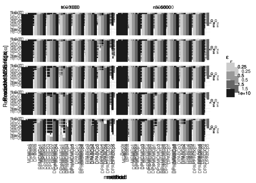
Figure 2: Rescaled median MSE for $\alpha$. The median is computed over all the MSE values obtained over the 50 simulated datasets and for each approach and combination of $(\bm{\alpha}^{\rm true},\epsilon,n)$. The non-private benchmarks MCMC and Boots are represented with the wider black bars.

Now, we focus on the scenarios where $\epsilon\in\{0.25,0.5,1.5\}$. The MSEs are decreasing in $\epsilon$ and $n$ and decreasing in $d$, which is to be expected. The methods DPapprox_p1,p3,p4 produce larger MSEs than the other methods and, for that reason, we discard them. We also exclude DPMCMC_p3, DPreMCMC_p3, and DPABC_p3 for similar reasons. The methods based on prior p3 produce similar results to priors p2, p4, and p5, which have the advantage of incorporating the prior dependence among $\bm{\alpha}$, which is not negligible. Since $p_{3}$ does not seem to be particularly advantageous and it ignores relevant structure, we discard it from further comparisons for simplicity.

The results with DPBoots are slightly worse than those for DPMCMC, while the results for DPABC are slightly worse than those for DPreMCMC, and DPreMCMC is, at the same time, also slightly worse than DPMCMC. All these small discrepancies diminish when $n$ or $\epsilon$ increase. We continue our analysis and comparisons using a representative for each of the Bayesian classes. Specifically, we choose DPMCMC_p1, DPreMCMC_p4, DPABC_p5.

Computation time is a key aspect to take into consideration, especially for the Bayesian approaches, as DPBoots is relatively fast. In the more challenging scenario with $n=5000$ and $\bm{\alpha}^{\rm true}_{5}$, which is the ideal approach, DPMCMC_p1 is relatively slow: approaches such as DPreMCMC_p4 and DPABC_p5 are approximately 6.2 (with $b=5$) and 60.3 times faster than DPMCMC_p1, respectively.

Figure 3 shows the MSEs for $E[\bm{x}|\bm{\alpha}]$ and the posterior predictive coverages. The MSEs for $E[\bm{x}|\bm{\alpha}]$ are all similar, and they are generally better than the MSEs we found for $\bm{\alpha}$.

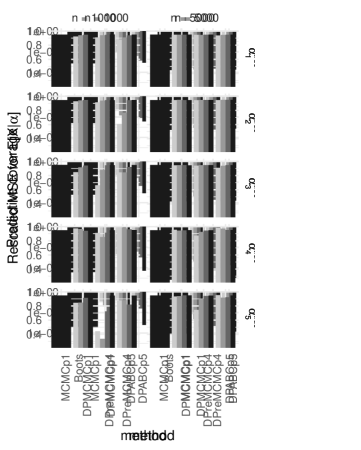
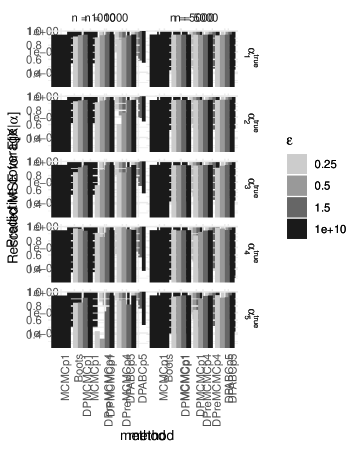
Figure 3: Left plot: Rescaled median MSE for $E[\bm{x}|\bm{\alpha}]$. The median is computed over all the MSE values obtained over the 50 simulated datasets and for each approach and combination of $(\bm{\alpha}^{\rm true},\epsilon,n)$. Right plot: Median posterior predictive coverage for the selected Bayesian approaches. The median is computed over all the coverage probabilities over the 50 simulated datasets and for each combination of $(\bm{\alpha}^{\rm true},\epsilon,n)$. In both plots, the non-private benchmarks MCMC and Boots are represented with the wider black bars.

Regarding the predictive coverage of the selected Bayesian methods, DPMCMC_p1 has better coverage than DPreMCMC_p4 and DPABC_p5. However, these discrepancies are diluted as $n$ and $\epsilon$ increase. This is especially evident for DPreMCMC_p4 and DPABC_p5.

We finish this section with some recommendations for users interested in implementing the methods. Users interested in non-Bayesian approaches can use DPBoots, which performs fairly well. For those interested in Bayesian approaches, if $n$ is small or $\epsilon<1$, we recommend DPMCMC_p1. Otherwise, if $n$ is large and $\epsilon\geq 1$, we recommend running both DPreMCMC_p4 and DPABC_p5. If these approaches agree, we can be confident that the results can be trusted. In general, we recommend users to proceed with caution if $n$ is large and $\epsilon<1$.

4.2 Application to Daily Time Spent

In this section, we apply our methods to a data set from the American Time Use Survey 2019 Microdata File, which we refer to as ATUS.

ATUS is collected and housed by the U.S. Bureau of Labor Statistics, and it comprises daily time spent in each of $18$ activities (e.g., sex, personal care, household activities, and helping household members) during 2019. The data set contains $9435$ records released by the U.S. Bureau of Labor Statistics on July 22, 2021.

We split up the data set between males and females and assume that $\bm{x}=(x_{1},x_{2},x_{3})$ is the fraction of time during the day spent on personal care $x_{1}$, eating and drinking $x_{2}$, and all other activities $x_{3}$. After removing missing values and individuals that spend no time on personal care or eating and drinking, the sample size is $7125$ observations ($3359$ males and $3766$ females). Conceptually, we assume that ATUS is a confidential data set, and that an analyst wants to use DP to test for differences between females and males. Specifically, we assume the analyst wants to test if such differences are greater than $0.01$, that is, $H_{0,j}:|E[x_{j}|{\rm Male}]-E[x_{j}|{\rm Female}]|\leq 0.01$ versus $H_{1,j}:|E[x_{j}|{\rm Male}]-E[x_{j}|{\rm Female}]|>0.01$ for $j\in\{1,2,3\}$.

We run the DP approaches DPBoots, DPMCMC_p1, DPreMCMC_p4 and DPABC_p5 a hundred times with $\epsilon=0.5$. We report our results in Table 2. The approaches are independently run for males and females. By Proposition 3, the privacy budget $\epsilon$ remains equal to $0.5$ after both analyses. To test these hypotheses, we use confidence intervals for DPBoots and posterior probabilities $\pi(H_{0,j}|S_{L}(\bm{D}_{2},a)=\bm{s}_{L}^{(2)},S_{L}(\bm{D}_{1},a)=\bm{s}_{L}^{(1)})$ for the Bayesian approaches. We report the average (over the 100 runs) expected time estimate for each activity, the fraction of times that DPBoots rejects the null hypothesis at significance level $0.05$, and the fraction of times the Bayesian approaches have posterior probabilities of the null hypothesis below $0.5$.

The estimates for the expected values under DP are similar to the benchmarks. Regarding testing $H_{0,j}$, we find that most of the times, the decision under DP and the benchmark is the same, with the exception of DPBoots and the activity related to eating and drinking. For this activity, while Boots rejects $H_{0,2}$, DPBoots fails to reject it. These types of discrepancies are common when testing hypotheses under DP because it injects additional uncertainty, which decreases the power of the tests. For Bayesian approaches, this phenomenon leads to posterior probabilities of $H_{0,j}$ shrinking to 0.5. In this application, we also experimented with different values of $\epsilon\geq 1$ and found out that $\epsilon$ needs to be around or greater than $1.25$ in order to make the decisions of Boots and DPBoots coincide. For all Bayesian approaches, the results for all hypotheses remain the same for $\epsilon\geq 0.5$, and the conclusion is that there is evidence of gender-based differences in the time spent on personal care and other activities, while there is no evidence of differences when eating and drinking. We also observe that in DP Bayesian approaches, the posterior probability of $H_{0,j}$ approach the results with MCMC_p1 as $\epsilon$ increases.

Table 2: Average mean time estimates for males and females and fraction of times that the null hypothesis is rejected (over 100 repetitions). Prob column shows the average (over 100 repetitions) posterior probability of the null hypothesis.

Method	Gender	Personal Care			Eating and drinking			Other activities
		Mean	Fraction	Prob	Mean	Fraction	Prob	Mean	Fraction	Prob
Boots	Female	0.411	1		0.0507	0		0.538	1
	Male	0.392			0.0508			0.557
DPBoots	Female	0.411	1		0.0512	1		0.538	1
	Male	0.392			0.0517			0.556
MCMCp1	Female	0.411	1	1e-5	0.0508	0	1	0.538	1	2e-5
	Male	0.392			0.0510			0.557
DPMCMCp1	Female	0.411	1	0.148	0.0508	0	0.907	0.538	1	0.191
	Male	0.392			0.0516			0.557
DPreMCMCp4	Female	0.411	1	0.143	0.0474	0.04	0.864	0.541	1	0.176
	Male	0.391			0.0484			0.561
DPABCp5	Female	0.413	1	0.249	0.0537	0.026	0.762	0.534	1	0.191
	Male	0.394			0.0540			0.553

For the Bayesian approaches, we also check the average posterior predictive distributions under DP for males and females. The results can be found in the Supplementary Material.

5 Discussion

In this work, we implemented and compared several approaches for analyzing compositional data under DP constraints that are based on the Dirichlet distribution.

We recommend using DPBoots for frequentist inference, which performs well in our experience. For Bayesian inference, we recommend implementing DPMCMC_p1 for small sample sizes or privacy budgets, and DPreMCMC_p4 and DPABC_p5 when both the sample size and the privacy budget are large. We recommend trusting the results with DPreMCMC_p4 and DPABC_p5 only when they give similar results.

A limitation of our work is that the Dirichlet distribution can be inadequate for some compositional data sets. Future work will use alternative models for compositional data.

This document contains supplemental materials to accompany the main manuscript. In Section S1, we provide the proof of Theorem 1, which states that Algorithm 1 satisfies $(\epsilon_{1}+\epsilon_{2})$-DP. In Section S2, we include a figure with the posterior predictive distributions estimated with the DP Bayesian methods for the ATUS application in Section 4.

S1 Proof Algorithm 1

Since $S_{G}(\bm{D})$ directly uses the Geometric mechanism, it satisfies $\epsilon_{2}$-DP. Hence, by Proposition 1, $A(S_{G}(\bm{D}))$ also satisfies $\epsilon_{2}$-DP. If $n_{1}=0$ (i.e., without partitioning), $S_{L}(\bm{D},a)$ is $\epsilon_{1}$-DP by the Laplace mechanism. Thus, sequential composition (Proposition 2) ensures that releasing both $S_{G}(\bm{D})$ and $S_{L}(\bm{D},a)$ satisfies $(\epsilon_{1}+\epsilon_{2})$-DP. If $n_{1}>0$ (i.e., with partitioning), releasing $S_{L}(\bm{D}_{1},a)$ and $S_{L}(\bm{D}_{2},a)$ is $\epsilon_{1}$-DP by the Laplace mechanism and parallel composition (Proposition 3). Thus, sequential composition ensures that releasing $S_{G}(\bm{D})$, $S_{L}(\bm{D}_{1},a)$, and $S_{L}(\bm{D}_{2},a)$ satisfies $(\epsilon_{1}+\epsilon_{2})$-DP.

S2 Posterior predictive distributions for ATUS data

In this section, we include the average posterior predictive distributions estimated with the DP Bayesian methods (averaged over the 100 runs).

Figure S1 displays the average of the estimated predictive distributions and histograms of the observed data. The posterior predictive densities are similar to the observed data, and the density estimates under DP are similar to those obtained through MCMC_p1.

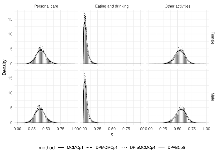
Figure S1: Posterior predictive distributions using DPreMCMC_p4 (with $\epsilon=1$) and MCMCp1 (benchmark) for males and females and each activity. Blue dashed lines represent 0.95 point-wise credible bands for DPreMCMC_p4. Histograms represent the observed data points.

References

- Aitchison (1982) Aitchison, J. (1982), “The statistical analysis of compositional data,” Journal of the Royal Statistical Society: Series B (Methodological), 44, 139–160.
- Awan and Slavkovic (2020) Awan, J. A. and Slavkovic, A. (2020), “Differentially private inference for binomial data,” Journal of Privacy and Confidentiality, 10.
- Bacon-Shone (2011) Bacon-Shone, J. (2011), “A short history of compositional data analysis,” Compositional data analysis: Theory and applications, 3–11.
- Barrientos et al. (2019) Barrientos, A. F., Reiter, J. P., Machanavajjhala, A., and Chen, Y. (2019), “Differentially private significance tests for regression coefficients,” Journal of Computational and Graphical Statistics, 28, 440–453.
- Bernstein and Sheldon (2018) Bernstein, G. and Sheldon, D. R. (2018), “Differentially private Bayesian inference for exponential families,” Advances in Neural Information Processing Systems, 31.
- Bernstein and Sheldon (2019) — (2019), “Differentially private Bayesian linear regression,” Advances in Neural Information Processing Systems, 32.
- Dwork et al. (2006) Dwork, C., McSherry, F., Nissim, K., and Smith, A. (2006), “Calibrating noise to sensitivity in private data analysis,” in Theory of cryptography conference, Springer, pp. 265–284.
- Efron (2012) Efron, B. (2012), “Bayesian inference and the parametric bootstrap,” The annals of applied statistics, 6, 1971.
- Ferrando et al. (2022) Ferrando, C., Wang, S., and Sheldon, D. (2022), “Parametric bootstrap for differentially private confidence intervals,” in International Conference on Artificial Intelligence and Statistics, PMLR, pp. 1598–1618.
- Ghosh et al. (2012) Ghosh, A., Roughgarden, T., and Sundararajan, M. (2012), “Universally utility-maximizing privacy mechanisms,” SIAM Journal on Computing, 41, 1673–1693.
- Inusah and Kozubowski (2006) Inusah, S. and Kozubowski, T. J. (2006), “A discrete analogue of the Laplace distribution,” Journal of statistical planning and inference, 136, 1090–1102.
- Ju et al. (2022) Ju, N., Awan, J. A., Gong, R., and Rao, V. A. (2022), “Data augmentation MCMC for Bayesian inference from privatized data,” arXiv preprint arXiv:2206.00710.
- Karwa and Vadhan (2017) Karwa, V. and Vadhan, S. (2017), “Finite sample differentially private confidence intervals,” arXiv preprint arXiv:1711.03908.
- Kifer and Machanavajjhala (2011) Kifer, D. and Machanavajjhala, A. (2011), “No free lunch in data privacy,” in Proceedings of the 2011 ACM SIGMOD International Conference on Management of data, pp. 193–204.
- Kulkarni et al. (2021) Kulkarni, T., Jälkö, J., Koskela, A., Kaski, S., and Honkela, A. (2021), “Differentially private Bayesian inference for generalized linear models,” in International Conference on Machine Learning, PMLR, pp. 5838–5849.
- Li et al. (2016) Li, N., Lyu, M., Su, D., and Yang, W. (2016), “Differential privacy: From theory to practice,” Synthesis Lectures on Information Security, Privacy, & Trust, 8, 1–138.
- Minka (2000) Minka, T. (2000), “Estimating a Dirichlet distribution,” Tech. rep., Massachusetts Institute of Technology.
- Minsker et al. (2017) Minsker, S., Srivastava, S., Lin, L., and Dunson, D. B. (2017), “Robust and scalable Bayes via a median of subset posterior measures,” Journal of Machine Learning Research, 18, 4488–4527.
- Narayanan (1991) Narayanan, A. (1991), “Algorithm AS 266: Maximum likelihood estimation of the parameters of the Dirichlet distribution,” Journal of the Royal Statistical Society. Series C (Applied Statistics), 365–374.
- Neal (2003) Neal, R. M. (2003), “Slice sampling,” The Annals of Statistics, 31, 705–767.
- Ongaro and Migliorati (2013) Ongaro, A. and Migliorati, S. (2013), “A generalization of the Dirichlet distribution,” Journal of Multivariate Analysis, 114, 412–426.
- Park et al. (2021) Park, M., Vinaroz, M., and Jitkrittum, W. (2021), “ABCDP: Approximate Bayesian computation with differential privacy,” Entropy, 23, 961.
- Park and Casella (2008) Park, T. and Casella, G. (2008), “The Bayesian LASSO,” Journal of the American Statistical Association, 103, 681–686.
- Peña and Barrientos (2021) Peña, V. and Barrientos, A. F. (2021), “Differentially private methods for managing model uncertainty in linear regression models,” arXiv preprint arXiv:2109.03949.
- Pritchard et al. (1999) Pritchard, J. K., Seielstad, M. T., Perez-Lezaun, A., and Feldman, M. W. (1999), “Population growth of human Y chromosomes: a study of Y chromosome microsatellites.” Molecular biology and evolution, 16, 1791–1798.
- Skorski (2023) Skorski, M. (2023), “Bernstein-type bounds for beta distribution,” Modern Stochastics: Theory and Applications, 10, 211–228.
- Srivastava et al. (2018) Srivastava, S., Li, C., and Dunson, D. B. (2018), “Scalable Bayes via barycenter in Wasserstein space,” Journal of Machine Learning Research, 19, 312–346.
- Sungur (2000) Sungur, E. A. (2000), “An introduction to copulas,” Journal of the American Statistical Association, 95, 334–334.
- Tavaré et al. (1997) Tavaré, S., Balding, D. J., Griffiths, R. C., and Donnelly, P. (1997), “Inferring coalescence times from DNA sequence data,” Genetics, 145, 505–518.
- Yao et al. (2022) Yao, Y., Vehtari, A., and Gelman, A. (2022), “Stacking for non-mixing Bayesian computations: The curse and blessing of multimodal posteriors,” Journal of Machine Learning Research, 23, 3426–3471.
Supplementary Material: Differentially Private Inference for Compositional Data
Qi Guo, Andrés F. Barrientos, and Víctor Peña333Qi Guo is Ph.D. candidate, Department of Statistics, Florida State University, USA (qg17@fsu.edu); Andrés F. Barrientos is Assistant Professor, Department of Statistics, Florida State University, USA (abarrientos@fsu.edu); Víctor Peña is a María Zambrano fellow, Department d’Estadística i Investigació Operativa,
Universitat Politècnica de Catalunya
Barcelona, Spain (victor.pena.pizarro@upc.edu).