Spectral Triadic Decompositions of Real-World Networks

Abstract

A fundamental problem in mathematics and network analysis is to find conditions under which a graph can be partitioned into smaller pieces. The most important tool for this partitioning is the Fiedler vector or discrete Cheeger inequality. These results relate the graph spectrum (eigenvalues of the normalized adjacency matrix) to the ability to break a graph into two pieces, with few edge deletions. An entire subfield of mathematics, called spectral graph theory, has emerged from these results. Yet these results do not say anything about the rich community structure exhibited by real-world networks, which typically have a significant fraction of edges contained in numerous densely clustered blocks. Inspired by the properties of real-world networks, we discover a new spectral condition that relates eigenvalue powers to a network decomposition into densely clustered blocks. We call this the spectral triadic decomposition. Our relationship exactly predicts the existence of community structure, as commonly seen in real networked data. Our proof provides an efficient algorithm to produce the spectral triadic decomposition. We observe on numerous social, coauthorship, and citation network datasets that these decompositions have significant correlation with semantically meaningful communities.

1 Introduction

The existence of clusters or community structure is one of the most fundamental properties of real-world networks. Across various scientific disciplines, be it biology, social sciences, or physics, the modern study of networks has often deal with the community structure of these data. Procedures that discover community structure have formed an integral part of network science algorithmics. Despite the large variety of formal definitions of a community in a network, there is broad agreement that it constitutes a dense substructure in an overall sparse network. Indeed, the discover of local density (also called clustering coefficients) goes back to the birth of network science.

Even beyond network science, graph partitioning is a central problem in applied mathematics and the theory of algorithms. Determining when such a partitioning is possible is a fundamental question that one straddles graph theory, harmonic analysis, differential geometry, and theoretical computer science. There is large body of mathematical and scientific research on how to break up a graph into smaller pieces.

Arguably, the most important mathematical tool for this partitioning problem is the discrete Cheeger inequality or the Fiedler vector. This result is the cornerstone of spectral graph theory and relates the eigenvalues of the graph Laplacian to the combinatorial structure. Consider an undirected graph $G=(V,E)$ with $n$ vertices. Let $d_{i}$ denote the degree of the vertex $i$. The normalized adjacency matrix, denoted ${\cal A}$, is the $n\times n$ matrix where the entry ${\cal A}_{ij}$ is $1/\sqrt{d_{i}d_{j}}$ if $(i,j)$ is an zero, and zero otherwise. (All diagonal entries are zero.) One can think of this entry as the “weight” of the edge between $i$ and $j$.

Let $\lambda_{1}\geq\lambda_{2}\ldots\geq\lambda_{n}$ denote the $n$ eigenvalues of the non-negative symmetric matrix ${\cal A}$. The largest eigenvalue $\lambda_{1}$ is always one. A basic fact is that $\lambda_{2}=1$ iff $G$ is disconnected. The discrete Cheeger inequality proves that if $\lambda_{2}$ is close to $1$ (has value $\geq 1-\varepsilon$), then $G$ is “close” to being disconnected. Formally, there exists a set $S$ of vertices that can be disconnected (from the rest of $G$) by removing an $O(\sqrt{\varepsilon})$-fraction of edges incident to $S$. The set of edges removed is called a low conductance cut.

We can summarize these observations as:

Basic fact:   Spectral gap is zero   $\Longrightarrow$   $G$ is disconnected
Cheeger bound:   Spectral gap is close to zero   $\Longrightarrow$   $G$ can be disconnected by low conductance set

The quantitative bound is one of the most important results in the study of graphs and network analysis. There is a rich literature of generalizing this bound for higher-order networks and simplicial complices. We note that many modern algorithms for finding communities in real-world networks are based on the Cheeger inequality in some form. The seminal Personalized PageRank algorithm is provides a local version of the Cheeger bound.

For modern network analysis and community structure, there are several unsatisfying aspects of the Cheeger inequality. Despite the variety of formal definitions of a community in a network, there is broad agreement that it constitutes many densely clustered substructures in an overall sparse network. The Cheeger inequality only talks of disconnecting $G$ into two parts. Even generalizations of the Cheeger inequality only work for a constant number of parts [5]. Real-world networks decompose into an extremely large of number of blocks/communities, and this number often scales with the network size[6, 11]. Secondly, the Cheeger bound works when the spectral gap is close to zero, which is often not true for real-world networks[6]. Real-world networks possess the small-world property[4]. But this property implies large spectral gap. Thirdly, Cheeger-type inequalities make no assertion on the interior of parts obtained. In community structure, we typically expect the interior to be dense and potentially assortative (possessing vertices of similar degree).

The main question that we address: is there a spectral quantity that predicts the existence of real-world community structure?

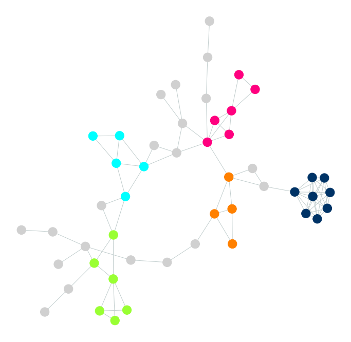
A toy decomposition

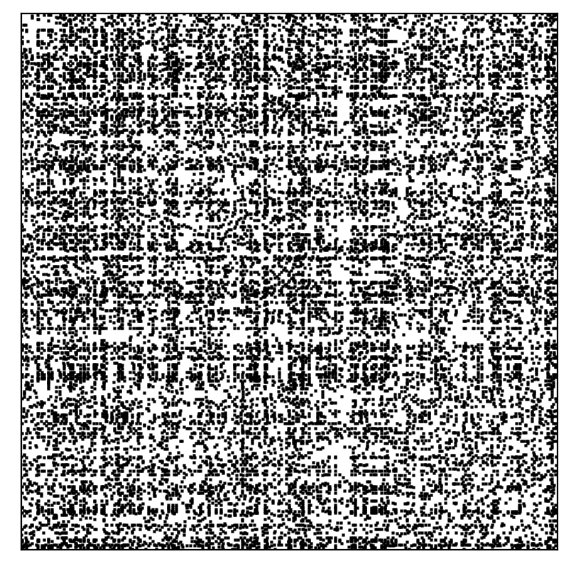
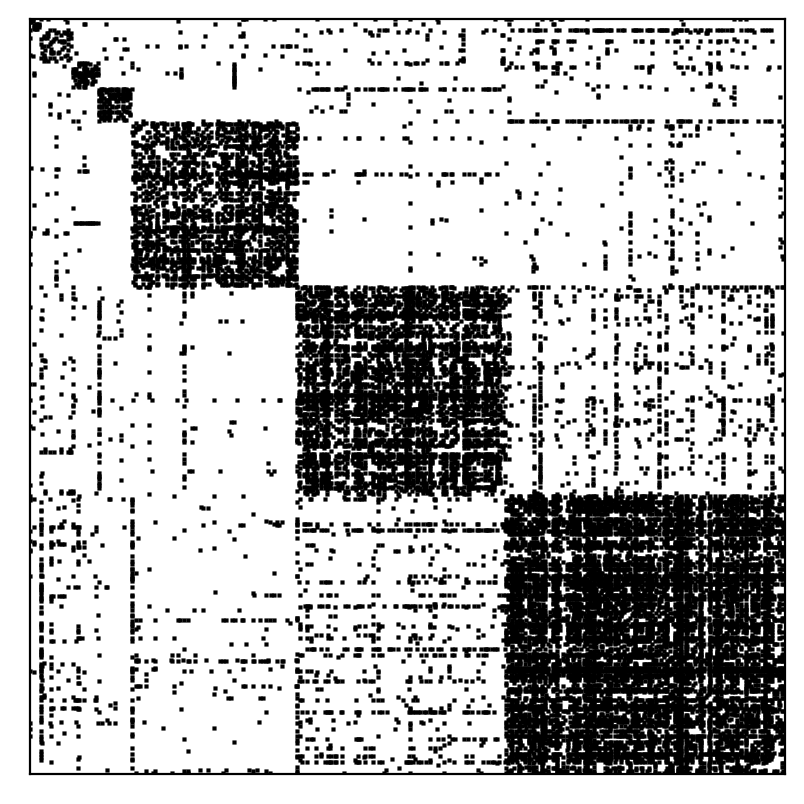
Original Subgraph

Subgraph ordered by extracted clusters

Figure 1: On the left, as a small example, we consider a subgraph induced by $155$ vertices and $\tau=0.49$ from a coauthorship network of Condensed Matter Physics researchers[9], and show a spectral triadic decomposition of the largest connected component, which has $49$ vertices. Each cluster is colored differently. We see how each cluster forms a densely connected component within an otherwise sparse graph. Also note that the clusters vary in size. The gray vertices do not participate in the decomposition, since they do not add significant to the cluster structure. On the right, we look at the adjacency matrices pre and post decomposition. The top figure is a spy plot of the adjacency matrix of 488 connected vertices from a Facebook network ([14],[13]) taken from the network repository[10], a graph with $\tau=0.122$. As a demonstration, we compute the spectral triadic decomposition of this subnetwork. We group the columns/rows by the clusters in the spy plot on the bottom. The latent community structure is immediately visible. Note that there exists many such blocks of varying sizes.

Our results:

We discover a new spectral relationship that addresses these issues. It predicts precisely the kind of community structure that is commonly observed in real-world networks, based on a quantity called the spectral transitivity.

Let $\lambda_{1}\geq\lambda_{2}\geq\ldots\lambda_{n}$ denote the spectrum (the eigenvalues) of the normalized adjacency matrix ${\cal A}$. We define the spectral transitivity, denoted $\tau$, as follows:

(1) $$\frac{\sum_{i\leq n}\lambda^{3}_{i}}{\sum_{i\leq n}\lambda^{2}_{i}}$$

The demoninator is the standard squared Frobenius norm of the matrix ${\cal A}$, while the numerator can be shown to be a weighted sum over the triangles in $G$ (refer to Claim 0.7 in the supplement). It can be seen as a weighted version of the standard transitivity, or global clustering coefficient[15]. (Other weighted versions have been defined in previous work[1].) It can be shown that the spectral transitivity $\tau$ is at least $1-1/(n-1)$. When $\tau$ has this maximum value, the graph is a perfect community, the $n$-clique. We mathematically prove that when $\tau$ is a constant (independent of graph size), then a constant fraction of the graph can be partitioned in dense, community-like structures. In the next section, we give a formal mathematical explanation. We summarize, analogous to the classic Cheeger inequality, as follows.
Basic fact:   $\tau$ is $1-1/(n-1)$ (the maximum)   $\Longrightarrow$   ${\cal A}$ is a perfectly clustered block.
Our discovery:    $\tau$ is at least constant   $\Longrightarrow$   Constant fraction of ${\cal A}$ is present in dense, clustered blocks.
For network analysis, the spectral transitivity $\tau$ takes the place of the spectral gap.

We find it remarkable that the value of a single quantity, the spectral transitivity, actually implies a global community structure of the graph. Moreover, we discover an efficient algorithm to produce these densely clustered blocks, which we call the spectral triadic decomposition. For convenience, we refer to a densely clustered block as a cluster. Unlike most community detection methods designed to a construct a few blocks, our theorem and algorithm produces thousands of clusters.

1.1 Significance

We give formalism for the decomposition and our main theorem in the next section. In this section, we explain the significance of our results for network science. The decomposition provided by our theorem has strong agreement with the conventional notion of a community structure. One gets many blocks, each with a guarantee on densely clustered internal structure. We notice an important deviation from standard Cheeger-like inequalities. Such bounds try to separate the graph by removing a few edges (or substructures). Most real-world networks have a significant fraction of long-rage edges or weak ties, that are not part of any community[8, 2, 4]. Hence, it makes more sense to try to find a constant fraction of the network within communities, rather than remove few edges to separate them.

Our insights have direct relevance to network analysis for real data. We observe that the $\tau$-values of a number of real-world networks are large. This data includes social networks, coauthorship networks, and citations networks (data in supplement). The $\tau$-values are typically in the range $0.1$ - $0.2$, even for networks with hundreds of thousands of edges. (For a random network of comparable size and similar degree distribution, the $\tau$-value would be $<10^{-5}$. That random graphs, even with high average degree, fail to capture triangle density is a well known fact[11].) We implemented our algorithm to compute the spectral triadic decomposition, and ran it on all these datasets.

We give pictorial depictions of the spectral triadic decomposition in Fig. 1. The image on the left shows a small snapshot of 155 vertices of a coauthorship network in Condensed Matter Physics [9] (the $\tau$ value is around $0.2$). As a toy example, we compute the spectral triadic decomposition of this network snapshot, and color the dense, clustered blocks in different colors. We can see how various pockets of density are automatically extracted by the spectral triadic decomposition. On the right, we show the adjacency matrix of a portion of a Facebook social network of college students at Rice University ([14, 13]) taken from the network repository[10] . We apply the spectral triadic decomposition and then order by blocks. The latent structure becomes immediately visible.

To state our main theorem, we first need to define the notion of approximately uniform matrices.

Definition 1.1.

Let $\alpha\in(0,1]$. A $k\times k$ zero diagonal non-negative matrix $M$ is called $\alpha$-uniform if at least an $\alpha$-fraction of non-diagonal entries have value in the range $[\alpha/(k-1),1/\alpha(k-1)]$.

For $s\in S$, let $N(s,S)$ denote the neighborhood of $s$ in $S$ (we define edges by non-zero entries). An $\alpha$-uniform matrix is strongly $\alpha$-uniform if for at least an $\alpha$-fraction of $s\in S$, $M|_{N(s,S)}$ is also $\alpha$-uniform.

Our main theorem is then the following (we restate it in more detail in §2).

Theorem 1.2.

Consider any normalized adjacency matrix ${\cal A}$ such that $\tau$ is at least a constant. Then, there exists a collection of disjoint sets of vertices $X_{1},X_{2},\ldots,X_{k}$ satisfying the following conditions:

• (Cluster structure) For all $i\leq k$, ${\cal A}|_{X_{i}}$ is strongly constant-uniform.

• (Coverage) $\sum_{i\leq k}\|{\cal A}|_{X_{i}}\|^{2}_{2}$ is $\Omega(\|{\cal A}\|^{2}_{2})$.

(All constants are polynomially related, independent of any graph parameter.)

1.2 High-level ideas of the proof

The full proof of Theorem 1.2 is mathematically involved with many moving parts. In this section, we highlight the key ideas, and make various simplifying assumptions. We note that the ideas are borrowed from a theoretical result of Gupta-Roughgarden-Seshadhri [3]. Their result talks about decompositions of triangle-dense graphs, but does not make any spectral connections. Moreover, their result works for the standard adjacency matrix, and cannot prove either bounds on strong uniformity or Frobenius norms (like Theorem 1.2). The GRS result does not have the analogies to the Cheeger inequality.

We begin by a combinatorial intepretation of the spectral clustering coefficient. Let $E$ be the set of edges and $T$ be the set of triangles in $G$. For a edge $e=(u,v)$, define the weight $\mathrm{wt}(e)$ to be $1/d_{u}d_{v}$. For a triangle $t=(u,v,w)$, define the weight $\mathrm{wt}(t):=1/(d_{u}d_{v}d_{w})$. Standard equalities show that $2\sum_{e\in E}\mathrm{wt}(e)=\sum_{i}\lambda^{2}_{i}$ and $\sum_{t\in T}\mathrm{wt}(t)=\sum_{i}\lambda^{3}_{i}$. We use the term “Frobenius weight” to refer to the squared Frobenius norm, since it is sum of weights of edges. Thus, the spectral clustering coefficient $\tau$, is the ratio of total weight of triangles to the total weight of edges (scaled by a factor of $3$).

The premise of Theorem 1.2 is that the total triangle weight of the graph is $(\tau/3)\sum_{e\in E}\mathrm{wt}(e)$. In this discussion, we will assume that $\tau$ is at least a constant, independent of graph size. So all dependencies on $\tau$ will be subsumed by the standard $O(\cdot),\Omega(\cdot)$ notation. The full proof has explicit dependencies on $\tau$. The decomposition of Theorem 1.2 is constructed by a procedure that repeatedly extracts the strongly uniform sets $X_{i}$. It maintains a subgraph $H=(V(H),E(H))$ under consideration. Initially, $H$ is set to the whole graph $G$. We use $T(H)$ to denote the set of triangles of $T$. A crucial definition is the notion of clean edges of $H$: an edge $e$ is clean if $\sum_{t\supset e:t\in T(H)}\mathrm{wt}(t)\geq(\tau/6)\mathrm{wt}(e)$. Thus, a clean edge is incident to a large amount of triangle weight, relative to its own weight.

We first prepare for the extraction step by repeatedly removing any unclean edge. Note that the removal of an unclean edge could remove triangles, which makes other edges unclean. The removals of unclean edges potentially cascade into many more removals. Nonetheless, observe that the removal of an unclean edge $e$ only removes at most $(\tau/6)\mathrm{wt}(e)$ triangle weight at the time of removal. The total triangle weight removed by all cleaning steps ever done is at most $(\tau/6)\sum_{e\in E}\mathrm{wt}(e)$, regardless of the order they are performed in. By definition, the total triangle weight in $G$ is exactly $(\tau/3)\sum_{e\in E}\mathrm{wt}(e)$. Hence, the cleaning steps still preserve at least half the total triangle weight.

So we end up with a graph $H$ that contains only clean edges. We will extract a strongly uniform set $X$ of vertices from $H$. An important decision is to begin the extraction from the lowest degree vertex $v$ that participates in $H$. The degree refers to the number of neighbors in the original graph $G$, not the subgraph $H$. The distinction is critical, since all edges/triangle weights are defined with respect to the original degree. We are trying to find uniform blocks in ${\cal A}$ (not in ${\cal A}$ restricted to $H$).

Pick any neighbor $u$ of $v$ in $H$. Since the edge $(u,v)$ is clean, the triangle weight that it is incident to (in $H$) is at least $\Omega(1/d_{u}d_{v})$ (the weight of $(u,v)$ is $1/d_{u}d_{v}$). Let $P(u)$, the partners of $u$, be the set of vertices that form a triangle with $(u,v)$ in $H$. We get:

(2) $$\sum_{w\in P(u)}(d_{u}d_{v}d_{w})^{-1}=\Omega((d_{u}d_{v})^{-1})\ \ \ \Longrightarrow\sum_{w\in P(u)}d^{-1}_{w}=\Omega(1)$$

Since all partners are also neighbors of $v$, the bound above implies that the average value of $d^{-1}_{w}$ is at least $\Omega(d^{-1}_{v})$. Using some algebra, we can prove that there are $\Omega(d_{v})$ neighbors of $v$ whose degree is $O(d_{v})$. We call these vertices the low degree neighbors, and denote them by $L$. An adaptation of the above argument proves that $\sum_{w\in P(u)\cap L}d^{-1}_{w}=\Omega(1)$.

We can apply this bound to prove that ${\cal A}|_{L}$ is constant-uniform. (Henceforth, we will simply say “uniform” to mean constant-uniform.) Observe that every edge in $L$ creates a triangle, so endpoints are partners of each other. Let us sum the weights of all edges in $L$ as follows and apply the bound $\sum_{w\in P(u)\cap L}d^{-1}_{w}=\Omega(1)$ twice:

(3) $$\sum_{u\in L}\sum_{w\in P(u)\cap L}(d_{u}d_{w})^{-1}=\sum_{u\in L}d^{-1}_{u}\Big{(}\sum_{w\in P(u)\cap L}d^{-1}_{w}\Big{)}=\Omega(\sum_{u\in L}d^{-1}_{u})=\Omega(1)$$

Thus, the sum of weights of edges in $L$ is $\Omega(1)$. Since $d_{v}$ is the lowest degree of any vertex in $H$, the maximum weight of an edge is at most $d^{-2}_{v}$. The size of $L$ is at most $d_{v}$, and there are at most $d^{2}_{v}$ edges in $L$. Hence, at least $\Omega(d^{2}_{v})$ edges in $L$ have weight $\Omega(d^{-2}_{v})$, implying that $L$ is uniform.

But we cannot extract $L$ as our desired set $X$, because $L$ might not be strongly uniform. Indeed, we have no guarantee of what the neighborhood of $u\in L$ restricted to $L$ looks like. To achieve strong uniformity, we need the set $X$ to contain sufficient triangle weight. Since $H$ is clean, all edges (of $H$) in $L$ are incident to significant triangle weight; but these triangles might not be contained in $L$. We add $L$ to the set $X$ to be extracted. Our next step is to find vertices that are neighbors of $L$ to add to $X$.

There is a delicate tradeoff here. We need to add vertices that will boost the triangle weight inside $X$, but adding too many vertices might affect the uniformity in $X$. Eventually, we need the matrices ${\cal A}|_{X_{i}}$ to contain enough Frobenius/edge weight (the coverage condition of Theorem 1.2). Note that the extraction on $X$ destroys Frobenius weight, because edges leaving $X$ get destroyed. So $X$ has to be chosen carefully to minimize this effect.

For all $w\in V(H)$, let us define $\rho_{w}$ to be the total triangle weight (in $H$) involving $w$ and an edge in $L$. Note that $\sum_{w}\rho_{w}$ is the total triangle weight involving edges from $L$. If we can capture a significant fraction of this total by adding a few vertices to $X$, we can ensure strong uniformity. First, since edges in $H$ are clean, we observe that $\sum_{w}\rho_{w}$ is large:

(4) $$\sum_{w}\rho_{w}=\sum_{e\subseteq L:e\in E(H)}\sum_{t\supset e:t\in T(H)}\mathrm{wt}(t)=\Omega(\sum_{e\subseteq L:e\in E(H)}\mathrm{wt}(e))$$

All vertices in $L$ have degree $O(d_{v})$, because there are all low-degree neighbors of $v$. Hence, all edge weights in $L$ are $\Omega(d^{-2}_{v})$. The uniformity of $L$ implies that there are $\Omega(d^{2}_{v})$ edges in $L$. Multiplying and plugging in (4), we deduce that $\sum_{w}\rho_{w}=\Omega(1)$. Remarkably, we can show that a few values of $\rho_{w}$ dominate the sum, which is crucial to the construction of $X$.

We will upper bound the sum $\sum_{w}\sqrt{\rho_{w}}$. The intuition is that when the $\rho_{w}$ values are concentrated on a few vertices, the sum of square roots becomes smaller. We can express $\rho_{w}$ as $\sum_{u,u^{\prime}\in L:(u,u^{\prime},w)\in T(H)}(d_{w}d_{u}d_{u^{\prime}})^{-1}\leq d^{-3}_{v}(\sum_{u\in L,(u,w)\in E(H)}1)^{2}$ (this is because $d_{v}$ is the smallest degree in $H$, and we can upper bound the LHS by a double summation). Let $c_{w}$ be the neighbors of $w$ in $L$ (in the graph $H$). We just bounded $\rho_{w}\leq d^{-3}_{v}c^{2}_{w}$, so $\sum_{w}\sqrt{\rho_{w}}\leq d^{-3/2}_{v}\sum_{w}c_{w}$. Observe that $\sum_{w}c_{w}$ basically counts edges that leave $L$, so it is at most $\sum_{u\in L}d_{u}$. The latter sum is at most $O(d^{2}_{v})$. Overall, we conclude that $\sum_{w}\sqrt{\rho_{w}}=O(d^{-3/2}_{v}\times d^{2}_{v})=O(\sqrt{d_{v}})$.

So we have the bound $\sum_{w}\rho_{w}=\Omega(1)$ and $\sum_{w}\sqrt{\rho_{w}}=O(\sqrt{d_{v}})$. Using some algebra, we can infer that there are $\Theta(d_{v})$ vertices $w$ such that $\rho_{w}=\Omega(d^{-1}_{v})$. We add these vertices to the set $X$; all the triangle weight corresponding to $\theta_{w}$ is now inside $X$. Note that $X$ still has size $O(d_{v})$, but the triangle weight contained in $X$ is at least $\Omega(1)$.

We can now prove that $X$ is strongly uniform. First, let us upper bound the triangle weight incident to any edge $(w,w^{\prime})$. Let $N(w)$ denote the neighborhood of $w$ in $H$. The triangle weight is at most

(5) $$\sum_{x\in N(w^{\prime})}(d_{w}d_{w^{\prime}}d_{x})^{-1}\leq(d_{w}d_{v})^{-1}\sum_{x\in N(w^{\prime})}d^{-1}_{w^{\prime}}=(d_{w}d_{v})^{-1}$$

Applying the above bound, the triangle weight incident to a vertex $w$ is at most

(6) $$\sum_{w^{\prime}\in N(w)}\sum_{t\supset(w,w^{\prime})}\mathrm{wt}(t)\leq\sum_{w^{\prime}\in N(w)}(d_{w}d_{v})^{-1}=d^{-1}_{v}$$

Since $X$ contains $\Omega(1)$ triangle weight, by the above bound, there must exist $\Omega(d_{v})$ vertices in $X$ incident to $\Omega(d^{-1}_{v})$ triangle weight inside $X$. Pick any such vertex $u$. The weight of a single triangle is at most $d^{-3}_{v}$. So $u$ must participate in $O(d^{2}_{v})$ triangles inside $X$. Since $|X|=O(d_{v})$, this implies that the neighborhood of $u$ in $X$ is also dense. We can also show that weights of edges in this neighborhood are $\Theta(d^{-2}_{v})$. Thus, ${\cal A}|_{N(u)\cap X}$ is a uniform matrix for every $u$ picked above. And ${\cal A}|_{X}$ is a strongly uniform matrix.

The final procedure extracts this $X$ from the graph $H$ and removes all edges leaving $X$. Then, the cleaning is performed again to prepare the “next” $H$, from which the next $X$ is extracted, and so on.

Proving the coverage bound: Note that the edge weight is precisely the contribution to the squared Frobenius norm. During the decomposition process, edge weight (which is Frobenius weight) is lost by edges that are cleaned, and by edges removed by the extraction process. We only preserve the Frobenius weight from edges completely contained in some $X_{i}$. We do not know how to directly bound the edge weight of the edges lost by cleaningFor an individual edge $e$ that is removed by cleaning, the triangle weight removed at that time will be much smaller than the edge weight.

But (as argued in the beginning of this section), we can bound the total triangle weight lost by cleaning. It turns out that, instead of tracking coverage through Frobenius/edge weight, it is easier to compute the triangle weight preserved. Using standard inequalities, we can then convert those bounds back in Frobenius weight.

Each set $X$ extracted has $O(d_{v})$ vertices and contains $\Omega(1)$ triangle weight. (Note that $d_{v}$ is the minimum degree vertices in the subgraph $H$ where $X$ was extracted. The value $d_{v}$ will change with each extraction.) Since any vertex in $H$ is incident to at most $d^{-1}_{v}$ triangle weight, the set $X$ is incident to at most $O(1)$ triangle weight. The ratio of triangle weight contained in $X$ to the triangle weight incident to $X$ is $\Omega(1)$. As argued in the beginning of this section, cleaning removes at most half the triangle weight. Thus, we can prove that the extracted sets contains an $\Omega(1)$ fraction of the total triangle weight. For each set $X_{i}$, standard bounds imply that the Frobenius weight is at least the triangle weight inside $X_{i}$. By the properties of spectral clustering coefficient, the total triange weight is at least the Frobenius weight. Putting it all together, the Frobenius weight inside the $X_{i}$s is at least to the total Frobenius weight of ${\cal A}$.

2 The Main Theorem

Our focus is entirely on non-negative matrices with zeroes on their diagonals. We are interested in the variation of values within submatrices of ${\cal A}$. Towards that, we define the following notion of approximately uniform matrices. We use $\|M\|_{2}$ to denote the Frobenius norm of a matrix. We restate our definition of approximately uniform matrices.

See 1.1

In an approximately uniform matrix, there are many entries of roughly the same (squared) value. Note that a $1$-uniform non-negative matrix has exactly the same value in all off-diagonal entries. A normalized adjacency matrix is $1$-uniform iff it represents a clique on $n$ vertices; hence, we can think of the uniformity parameter $\alpha$ as a measure of how “clique-like” an adjacency matrix is.

To motivate our main theorem, let us a prove a basic spectral fact regarding $\tau({\cal A})$.

Lemma 2.1.

Consider normalized adjacency matrices ${\cal A}$ of dimension $n$. The maximum value of $\tau({\cal A})$ is $1-1/(n-1)$. Moreover, this value is attained for a unique strongly $1$-regular matrix, the normalized adjacency matrix of the $n$-clique.

Proof.

First, consider the normalized adjacency matrix ${\cal A}$ of the $n$-clique. All off-diagonal entries are precisely $1/(n-1)$ and ${\cal A}$ can be expressed as $(n-1)^{-1}({\bf 1}{\bf 1}^{T}-I)$. The matrix ${\cal A}$ is $1$-regular. The largest eigenvalue is $1$ and all the remaining eigenvalues are $-1/(n-1)$. Hence, $\sum_{i}\lambda^{3}_{i}=1-(n-1)/(n-1)^{3}=1-1/(n-1)^{2}$. The sum of squares of eigenvalue is $\sum_{i}\lambda^{3}_{i}=1+(n-1)/(n-1)^{2}=1+1/(n-1)$. Dividing,

$$\frac{\sum_{i\leq n}\lambda^{3}_{i}}{\sum_{i\leq n}\lambda^{2}_{i}}=1-1/(n-1).$$

Since the matrix has zero diagonal, the trace $\sum_{i}\lambda_{i}$ is zero. We will now prove the following claim.

Claim 2.2.

Consider any sequence of numbers $1=\lambda_{1}\geq\lambda_{2}\ldots\geq\lambda_{n}$ such that $\forall i,|\lambda_{i}|\leq 1$ and $\sum_{i}\lambda_{i}=0$. If $\sum_{i}\lambda^{3}_{i}\geq(1-1/(n-1))\sum_{i}\lambda^{2}_{i}$, then $\forall i>1,\lambda_{i}=-1/(n-1)$.

Proof.

Let us begin with some basic manipulations.

(7) $$\sum_{i}\lambda^{3}_{i}\geq[1-1/(n-1)]\sum_{i}\lambda^{2}_{i}\ \ \ \Longrightarrow\ \ \ 1+\sum_{i>1}\lambda^{3}_{i}\geq[1-1/(n-1)]\cdot(1+\sum_{i>1}\lambda^{2}_{i})$$

$$\Longrightarrow\ \ \ \sum_{i>1}\lambda^{3}_{i}\geq[1-1/(n-1)]\sum_{i>1}\lambda^{2}_{i}-1/(n-1)$$

For $i>1$, define $\delta_{i}:=\lambda_{i}+1/(n-1)$. Note that $\sum_{i>1}\lambda_{i}=-1$, so $\sum_{i>1}\delta_{i}=0$. Moreover, $\forall i>1$, $\delta_{i}\leq 1+1/(n-1)$. We plug in $\lambda_{i}=\delta_{i}-1/(n-1)$ in (7).

$$\sum_{i>1}\Big{[}\delta_{i}-1/(n-1)\Big{]}^{3}\geq[1-1/(n-1)]\sum_{i>1}\Big{[}\delta_{i}-1/(n-1)\Big{]}^{2}-1/(n-1)$$

$$\Longrightarrow\sum_{i>1}\Big{[}\delta^{3}_{i}-3\delta^{2}_{i}/(n-1)+3\delta_{i}/(n-1)^{2}-1/(n-1)^{3}\Big{]}\geq[1-1/(n-1)]\sum_{i>1}\Big{[}\delta^{2}_{i}-2\delta_{i}/(n-1)+1/(n-1)^{2}\Big{]}-1/(n-1)$$

Recall that $\sum_{i>1}\delta_{i}=0$. Hence, we can simplify the above inequality.

$$\sum_{i>1}\delta^{3}_{i}-(3/(n-1))\sum_{i>1}\delta^{2}_{i}-1/(n-1)^{2}\geq[1-1/(n-1)]\sum_{i>1}\delta^{2}_{i}+1/(n-1)-1/(n-1)^{2}-1/(n-1)$$

$$\Longrightarrow\sum_{i>1}\delta^{3}_{i}\geq[1+2/(n-1)]\sum_{i>1}\delta^{2}_{i}\ \ \ \ \textrm{(Canceling terms and rearranging)}$$

Since $\delta_{i}\leq(1+1/(n-1))$, we get that $\sum_{i>1}\delta^{3}_{i}\leq[1+1/(n-1)]\sum_{i>1}\delta^{2}_{i}$. Combining with the above inequality, we deduce that $[1+2/(n-1)]\sum_{i>1}\delta^{2}_{i}\leq[1+1/(n-1)]\sum_{i>1}\delta^{2}_{i}$. This can only happen if $\sum_{i>1}\delta^{2}_{i}$ is zero, implying all $\delta_{i}$ values are zero. Hence, for all $i>1$, $\lambda_{i}=-1/(n-1)$. ∎

With this claim, we conclude that any matrix ${\cal A}$ maximizing the ratio of cubes and squares of eigenvalues has a fixed spectrum. It remains to prove that a unique normalized adjacency matrix has this spectrum. We use the rotational invariance of the Frobenius norm: sum of squares of entries of ${\cal A}$ is the same as the sum of squares of eigenvalues. Thus,

(8) $$\sum_{(u,v)\in E}\frac{2}{d_{u}d_{v}}=1-1/(n-1)=n/(n-1)$$

Observe that $\frac{2}{d_{u}d_{v}}\geq 1/(d_{u}(n-1))+1/(d_{v}(n-1))$, since all degrees are at most $n-1$. Summing this inequality over all edges,

$$\sum_{(u,v)\in E}\frac{2}{d_{u}d_{v}}\geq\sum_{v\in V}\sum_{u\in N(v)}\frac{1}{d_{v}(n-1)}=\sum_{v\in V}\frac{d_{v}}{d_{v}(n-1)}=n/(n-1)$$

Hence, for (8) to hold, for all edges $(u,v)$, we must have the equality $\frac{2}{d_{u}d_{v}}=1/(d_{u}(n-1))+1/(d_{v}(n-1))$. That implies that for all edge $(u,v)$, $d_{u}=d_{v}=n-1$. So all vertices have degree $(n-1)$, and the graph is an $n$-clique. ∎

Our main theorem is a generalization of Lemma 2.1. Since we focus on an arbitrary fixed matrix ${\cal A}$, we will simply use $\tau$ to denote $\tau({\cal A})$. We prove that when the ratio of powers of eigenvalues is at least a constant, a constant fraction of the (Frobenius norm of the) matrix ${\cal A}$ is contained in approximately uniform matrices. Thus, all matrices having a large spectral triadic content possess a decomposition of ${\cal A}$ into approximately uniform matrices.

Theorem 2.3 (Main Theorem).

There exist absolute constants $\delta>0$ and $c>0$ such that the following holds. Consider any normalized adjacency matrix ${\cal A}$. There exists a collection of disjoint sets of vertices $X_{1},X_{2},\ldots,X_{k}$ satisfying the following conditions:

• (Cluster structure) For all $i\leq k$, ${\cal A}|_{X_{i}}$ is strongly $\delta\tau^{c}$-uniform.

• (Coverage) $\sum_{i\leq k}\|{\cal A}|_{X_{i}}\|^{2}_{2}\geq\delta\tau^{c}\|{\cal A}\|^{2}_{2}$.

3 Preliminaries

We use $V,E,T$ to denote the sets of vertices, edges, and triangles of $G$, respectively. For any subgraph $H$ of $G$, we use $V_{H},E_{H},T_{H}$ to denote the corresponding sets within $H$. For any edge $e$, let $T_{H}(e)$ denote the set of triangles in $H$ containing $e$.

For any vertex $v$, let $d_{v}$ denote the degree of $v$ (in $G$).

We first define the notion of weights for edges and triangles. We will think of edges and triangles as unordered sets of vertices.

Definition 3.1.

For any edge $e=(u,v)$, define the weight $\mathrm{wt}(e)$ to be $\frac{1}{d_{u}d_{v}}$. For any triangle $t=(u,v,w)$, define the weight $\mathrm{wt}(t)$ to be $\frac{1}{d_{u}d_{v}d_{w}}$.

For any set $S$ consisting solely of edges or triangles, define $\mathrm{wt}(S)=\sum_{s\in S}\mathrm{wt}(s)$.

We state some basic facts that relate the sum of weights to sum of eigenvalue powers. Let $S\subset V$ be any subset of vertices, and let ${\cal A}|_{S}$ denote the submatrix of ${\cal A}$ restricted to $S$. We use $\lambda_{i}(S)$ to denote the $i$th largest eigenvalue of the symmetric submatrix ${\cal A}|_{S}$. Abusing notation, we use $E_{S}$ and $T_{S}$ to denote the edges and triangles contained in the graph induced on $S$.

Claim 3.2.

$\sum_{i\leq|S|}\lambda^{2}(S)_{i}=2\sum_{e\in E(S)}\mathrm{wt}(e)$

Proof.

By the properties of the Frobenius norm of matrices, $\sum_{i\leq|S|}\lambda^{2}_{i}=\sum_{s,t\in S}{\cal A}^{2}_{s,t}$ Note that ${\cal A}_{s,t}=A_{s,t}/\sqrt{d_{s}d_{t}}$. Hence, $\sum_{s,t}{\cal A}^{2}_{s,t}=2\sum_{e=(u,v)\in E(S)}1/d_{u}d_{v}$. (We get a $2$-factor because each edge $(u,v)$ appears twice in the adjacency matrix.) ∎

Claim 3.3.

$\sum_{i\leq|S|}\lambda^{3}(S)_{i}=6\sum_{t\in T(S)}\mathrm{wt}(t)$.

Proof.

Note that $\sum_{i\leq|S|}\lambda^{3}(S)_{i}$ is the trace of $({\cal A}|_{S})^{3}$. The diagonal entry $({\cal A}|_{S})^{3}_{ii}$ is precisely $\sum_{s\in S}\sum_{s^{\prime}\in S}{\cal A}_{is}{\cal A}_{ss^{\prime}}{\cal A}_{s^{\prime}i}$. Note that ${\cal A}_{is}{\cal A}_{ss^{\prime}}{\cal A}_{s^{\prime}i}$ is non-zero iff $(i,s,s^{\prime})$ form a triangle. In that case, ${\cal A}_{is}{\cal A}_{ss^{\prime}}{\cal A}_{s^{\prime}i}=1/\sqrt{d_{i}d_{s}}\cdot 1/\sqrt{d_{s}d_{s^{\prime}}}\cdot 1/\sqrt{d_{s^{\prime}}d_{i}}=\mathrm{wt}((i,s,s^{\prime}))$, We conclude that $({\cal A}|_{S})^{3}_{ii}$ is $2\sum_{t\in T(S),t\ni i}\mathrm{wt}(t)$. (There is a $2$ factor because every triangle is counted twice.)

Thus, $\sum_{i\leq n}\lambda^{3}(S)_{i}=\sum_{i}2\sum_{t\in T,t\ni i}\mathrm{wt}(t)=2\sum_{t\in T}\sum_{i\in t}\mathrm{wt}(t)=6\sum_{t\in T}\mathrm{wt}(t)$. (The final $3$ factor appears because a triangle contains exactly $3$ vertices.) ∎

Claim 3.4.

$\sum_{t\in T(S)}\mathrm{wt}(t)\leq\|{\cal A}|_{S}\|^{2}_{2}/6$.

Proof.

By Claim 3.3 $\sum_{t\in T(S)}\mathrm{wt}(t)=\sum_{i\leq|S|}\lambda^{3}(S)_{i}/6$. The maximum eigenvalue of ${\cal A}$ is $1$, and since ${\cal A}|_{S}$ is a submatrix, $\lambda(S)_{1}\leq 1$ (Cauchy’s interlacing theorem). Thus, $\sum_{i\leq|S|}\lambda^{3}(S)_{i}\leq\sum_{i\in|S|}\lambda^{2}(S)_{i}=\|{\cal A}|_{S}\|^{2}_{2}$. ∎

As a direct consequence of the previous claims applied on ${\cal A}$, we get the following characterization of the spectral triadic content in terms of the weights.

Lemma 3.5.

$\tau=\frac{3\sum_{t\in T}\mathrm{wt}(t)}{\sum_{e\in E}\mathrm{wt}(e)}$.

We will need the following “reverse Markov inequality”.

Lemma 3.6.

Consider a random variable $Z$ taking values in $[0,b]$. If $\hbox{\bf E}[Z]\geq\sigma b$, then $\Pr[Z\geq\sigma b/2]\geq\sigma/2$.

Proof.

In the following calculations, we will upper bound the conditional expectation by the maximum value (under that condition).

(9) $$\sigma b\leq\hbox{\bf E}[Z]=\Pr[Z\geq\sigma b/2]\cdot\hbox{\bf E}[Z|Z\geq\sigma b/2]+\Pr[Z\leq\sigma b/2]\cdot\hbox{\bf E}[Z|Z\leq\sigma b/2]\leq\Pr[Z\geq\sigma b/2]\cdot b+\sigma b/2$$

We rearrange to complete the proof. ∎

4 Cleaned graphs and extraction

For convenience, we set $\varepsilon=\tau/6$.

Definition 4.1.

A connected subgraph $H$ is called clean if $\forall e\in E(H)$, $\mathrm{wt}(T_{H}(e))\geq\varepsilon{}\mathrm{wt}(e)$.

Algorithm 1 Extract$(H)$

1:Pick $v\in V(H)$ that minimizes $d_{v}$.

2:Construct the set $L:=\{u|(u,v)\in E(H),d_{u}\leq 2\varepsilon^{-1}d_{v}\}$ ($S$ is the set of low degree neighbors of $v$ in $H$.)

3:For every vertex $w\in V(H)$, define $\rho_{w}$ to be the total weight of triangles of the form $(w,u,u^{\prime})$ where $u,u^{\prime}\in L$.

4:Sort the vertices in decreasing order of $\rho_{w}$, and construct the “sweep cut” $C$ to be the smallest set satisfying $\sum_{w\in C}\rho_{w}\geq(1/2)\sum_{w\in V(H)}\rho_{w}$.

5:Output $X:=\{v\}\cup L\cup C$.

The main theorem of this section follows.

Theorem 4.2.

Suppose the subgraph $H$ is connected and clean. Let $X$ denote the output of the procedure Extract$(H)$. Then

$$\sum_{t\in T(H),t\subseteq X}\mathrm{wt}(t)\geq(\varepsilon^{8}/2000)\sum_{t\in T(H),t\cap X\neq\emptyset}\mathrm{wt}(t)$$

(The triangle weight contained inside $X$ is a constant fraction of the triangle weight incident to $X$.)

Moreover, ${\cal A}|_{X}$ is strongly $\delta\varepsilon^{12}$-uniform.

We will need numerous intermediate claims to prove this theorem. We use $v$, $L$, and $C$ as defined in Extract$(H)$. We use $N$ to denote the neighborhood of $v$ in $H$. Note that $L\subseteq N$.

For any vertex $u\in N$, we define the set of partners $P(u)$ to be $\{w:(u,v,w)\in T_{H}\}$.

The following lemma is an important tool in our analysis.

Lemma 4.3.

For any $u\in N$, $\sum_{w\in P(u)\cap L}d^{-1}_{w}\geq\varepsilon/2$.

Proof.

Let $e=(u,v)$. Since $H$ is clean, $\mathrm{wt}(T_{H}(e))\geq\varepsilon\mathrm{wt}(e)$. Expanding out the definition of weights,

(10) $$\sum_{w:(u,v,w)\in T_{H}}\frac{1}{d_{u}d_{v}d_{w}}\geq\frac{\varepsilon}{d_{u}d_{v}}\ \ \ \Longrightarrow\ \ \ \sum_{w\in P(u)}{d^{-1}_{w}}\geq\varepsilon$$

Note that $L$ (as constructed in Extract$(H)$) is the subset of $N$ consisting of vertices with degree at most $2\varepsilon^{-1}d_{v}$. For $w\in N\setminus L$, we have the lower bound $d_{w}\geq 2\varepsilon^{-1}d_{v}$. Hence,

(11) $$\sum_{w\in N\setminus L}d^{-1}_{w}\leq|N\setminus L|(\varepsilon/2)d^{-1}_{v}\leq d_{v}\times(\varepsilon/2)d^{-1}_{v}=\varepsilon/2.$$

In the calculation below, we split the sum of (10) into the contribution from $L$ and from outside $L$. We apply (11) to bound the latter contribution.

$$\varepsilon\leq\sum_{w\in P(u)}d^{-1}_{w}\leq\sum_{w\in P(u)\cap L}d^{-1}_{w}+\sum_{w\in N\setminus L}d^{-1}_{w}\leq\sum_{w\in P(u)\cap L}d^{-1}_{w}+\varepsilon/2$$

∎

Claim 4.4.

$|L|\geq\varepsilon d_{v}/2$

Proof.

Since $H$ is connected, there must exist some edge $e=(u,v)\in E(H)$. By Lemma 4.3, $\sum_{w\in P(u)\cap L}d^{-1}_{w}\geq\varepsilon/2$. Hence, $\sum_{w\in L}d^{-1}_{w}\geq\varepsilon/2$. Since $v$ is the vertex in $V(H)$ minimizing $d_{v}$, for any $w\in V(H)$, $d_{w}\geq d_{v}$. Thus,

$$\varepsilon/2\leq\sum_{w\in L}d^{-1}_{w}\leq\sum_{w\in L}d^{-1}_{v}=|L|d^{-1}_{v}$$

∎

Claim 4.5.

$\sum_{e\in E(H),e\subseteq L}\mathrm{wt}(e)\geq\varepsilon^{2}/8$.

Proof.

By Lemma 4.3, $\forall w\in L$, $\sum_{w^{\prime}\in P(w)\cap L}d^{-1}_{w^{\prime}}\geq\varepsilon/2$. We multiply both sides by $d^{-1}_{w}$ and sum over all $w\in L$.

$$\sum_{w\in L}\sum_{w^{\prime}\in P(w)\cap L}(d_{w}d_{w^{\prime}})^{-1}\geq(\varepsilon/2)\sum_{w^{\prime}\in L}d^{-1}_{w^{\prime}}$$

By Lemma 4.3, $\sum_{w^{\prime}\in L}d^{-1}_{w^{\prime}}\geq\varepsilon/2$. Note that $w^{\prime}\in P(w)$ only if $(w,w^{\prime})\in E(H)$. Hence,

$\sum_{w\in L}\sum_{w^{\prime}\in L,(w,w^{\prime})\in E(H)}\mathrm{wt}((w,w^{\prime}))\geq\varepsilon^{2}/4$. Note that the summation counts all edges twice, so we divide by $2$ to complete the proof. ∎

We now come to the central calculations of the main proof. Recall, from the description of Extract, that $\rho_{w}$ is the total triangle weight of the triangles $(w,u,u^{\prime})$, where $u,u^{\prime}\in L$. We will prove that $\sum_{w}\rho_{w}$ is large; moreover, there are a few entries that dominate the sum. The latter bound is crucial to arguing that the sweep set $C$ is not too large.

Claim 4.6.

$\sum_{w\in V(H)}\rho_{w}\geq\varepsilon^{3}/8$.

Proof.

Note that $\sum_{w\in V(H)}\rho_{w}$ is equal to $\sum_{e\in E(H),e\subset L}\mathrm{wt}(T_{H}(e))$. Both these expressions give the total weight of all triangles in $H$ that involve two vertices in $L$. Since $H$ is clean, for all edges $e\in E(H)$, $\mathrm{wt}(T_{H}(e))\geq\varepsilon\mathrm{wt}(e)$. Hence, $\sum_{e\in E(H),e\subset L}\mathrm{wt}(T_{H}(e))\geq\varepsilon\sum_{e\in E(H),e\subset L}\mathrm{wt}(e)$. Applying Claim 4.5, we can lower bound the latter by $\varepsilon^{3}/8$. ∎

We now show that a few $\rho_{w}$ values dominate the sum, using a somewhat roundabout argument. We upper bound the sum of square roots.

Claim 4.7.

$\sum_{w\in V(H)}\sqrt{\rho_{w}}\leq 2\varepsilon^{-1}\sqrt{d_{v}}$

Proof.

Let $c_{w}$ be the number of vertices in $L$ that are neighbors (in $H$) of $w$. Note that for any triangle $(u,u^{\prime},w)$ where $u,u^{\prime}\in L$, both $u$ and $u^{\prime}$ are common neighors of $w$ and $v$. The number of triangles $(u,u^{\prime},w)$ where $u,u^{\prime}\in L$ is at most $c^{2}_{w}$. The weight of any triangle in $H$ is at most $d^{-3}_{v}$, since $d_{v}$ is the lowest degree (in $G$) of all vertices in $H$. As a result, we can upper bound $\rho_{w}\leq d^{-3}_{v}c^{2}_{w}$.

Taking square roots and summing over all vertices,

(12) $$\sum_{w\in V(H)}\sqrt{\rho_{w}}\leq d^{-3/2}_{v}\sum_{w\in V(H)}c_{w}$$

Note that $\sum_{w\in V(H)}c_{w}$ is exactly the sum over $u\in L$ of the degrees of $u$ in the subgraph $H$. (Every edge incident to $u\in L$ gives a unit contribution to the sum $\sum_{w\in V(H)}c_{w}$.) By definition, every vertex in $L$ has degree in $H$ at most $2\varepsilon^{-1}d_{v}$. The size of $L$ is at most $d_{v}$.

Hence, $\sum_{w\in V(H)}c_{w}\leq 2\varepsilon^{-1}d^{2}_{v}$. Plugging into (12), we deduce that $\sum_{w\in V(H)}\sqrt{\rho_{w}}\leq 2\varepsilon^{-1}\sqrt{d_{v}}$. ∎

We now prove that the sweep cut $C$ is small, which is critical to proving Theorem 4.2.

Claim 4.8.

$|C|\leq 144\varepsilon^{-5}d_{v}$.

Proof.

For convenience, let us reindex vertices so that $\rho_{1}\geq\rho_{2}\geq\rho_{3}\ldots$. Let $r\leq n$ be an arbitrary index. Because we index in non-increasing order, note that $\sum_{j\leq n}\rho_{j}\geq r\rho_{r}$. Furthermore, $\forall j>r$, $\rho_{j}\leq\rho_{r}$.

(13) $$\sum_{j>r}\rho_{j}\leq\sqrt{\rho_{r}}\sum_{j>r}\sqrt{\rho_{j}}\leq\sqrt{\frac{\sum_{j\leq n}\rho_{j}}{r}}\sum_{j\leq n}\sqrt{\rho_{j}}=\Big{[}\frac{\sum_{j\leq n}\sqrt{\rho_{j}}}{\sqrt{r}\cdot\sqrt{\sum_{j\leq n}\rho_{j}}}\Big{]}\sum_{j\leq n}\rho_{j}$$

Observe that Claim 4.7 gives an upper bound on the numerator, while Claim 4.6 gives a lower bound on (a term in) the demonimator. Plugging those bounds in (13),

$$\sum_{j>r}\rho_{j}\leq\frac{2\varepsilon^{-1}\sqrt{d_{v}}}{\sqrt{r}\cdot\varepsilon^{3/2}/\sqrt{8}}\sum_{j\leq n}\rho_{j}\leq\frac{1}{\sqrt{r}}\cdot\frac{6\sqrt{d_{v}}}{\varepsilon^{5/2}}\cdot\sum_{j\leq n}\rho_{j}$$

Suppose $r>144\varepsilon^{-5}d_{v}$. Then $\sum_{j>r}\rho_{j}<(1/2)\sum_{j\leq n}\rho_{j}$. The sweep cut $C$ is constructed with the smallest value of $r$ such that $\sum_{j>r}\rho_{j}<(1/2)\sum_{j\leq n}\rho_{j}$. Hence, $|C|\leq 144\varepsilon^{-5}d_{v}$. ∎

An additional technical claim we need bounds the triangle weight incident to a single vertex.

Claim 4.9.

For all vertices $u\in V(H)$, $\mathrm{wt}(T_{H}(u))\leq(2d_{v})^{-1}$.

Proof.

Consider edge $(u,w)\in E(H)$. We will prove that $\mathrm{wt}(T_{H}((u,w)))\leq\delta^{-1}_{u}d^{-1}_{v}$. Recall that $d_{v}$ is the smallest degree among vertices in $H$. Furthermore, $|T_{H}((u,w))|\leq d_{w}$, since the third vertex in a triangle containing $(u,w)$ is a neighbor of $w$.

$$\mathrm{wt}(T_{H}((u,v)))=\sum_{z:(z,u,w)\in T(H)}\frac{1}{d_{u}d_{w}d_{z}}\leq\frac{1}{d_{u}d_{v}}\sum_{z:(z,u,w)\in T(H)}\frac{1}{d_{w}}\leq\frac{1}{\delta_{u}d_{v}}\times\frac{d_{w}}{d_{w}}=\frac{1}{d_{u}d_{v}}$$

We now bound $\mathrm{wt}(T_{H}(u))$ by summing over all neighbors of $u$ in $H$.

$$\mathrm{wt}(T_{H}(u))=(1/2)\sum_{w:(u,w)\in E(H)}\mathrm{wt}(T_{H}((u,w)))\leq(1/2)\sum_{w:(u,w)\in E(H)}\frac{1}{d_{u}d_{v}}=\frac{1}{2d_{v}}\sum_{w:(u,w)\in E(H)}\frac{1}{d_{u}}\leq\frac{1}{2d_{v}}\times\frac{d_{u}}{d_{u}}=\frac{1}{2d_{v}}$$

∎

4.1 The proof of Theorem 4.2

Proof.

(of Theorem 4.2) By construction of $X$ as $\{v\}\cup L\cup C$, all the triangles of the form $(w,u,u^{\prime})$, where $w\in C$ and $u,u^{\prime}\in L$, are contained in $X$. The total weight of such triangles is at least $\sum_{v\leq n}\rho_{v}/2$, by the construction of $C$. By Claim 4.6, $\sum_{v\leq n}\rho_{v}/2\geq\varepsilon^{3}/16$.

Let us now bound that total triangle weight incident to $X$ in $H$. Observe that $|X|=1+|L|+|C|$ which is at most $1+d_{v}+\varepsilon^{-5}144d_{v}$, by Claim 4.8. We can further bound $|X|\leq\varepsilon^{-5}146d_{v}$. By Claim 4.9, the total triangle weight incident to a vertex is at most $(2d_{v})^{-1}$. Hence, the total triangle weight incident to all of $X$ is at most $73\varepsilon^{-5}$.

Thus, the triangle weight contained in $X$ is at least $\frac{\varepsilon^{3}/16}{73\varepsilon^{-5}}$ times the triangle weight incident to $X$. The ratio is at least $\varepsilon^{8}/2000$, completing the proof of the first statement.

Proof of uniformity of ${\cal A}|_{X}$: We first prove a lower bound on the uniformity of ${\cal A}|_{X}$. For convenience, let $B$ denote the set $\{e|e\in E(H),e\subseteq L$. By Claim 4.5, $\sum_{e\in B}\mathrm{wt}(e)\geq\varepsilon^{2}/8$. There are at most ${d_{v}\choose 2}\leq d^{2}_{v}/2$ edges in $B$. For every edge $e$, $\mathrm{wt}(e)\leq 1/d^{2}_{v}$. Let $k$ denote the number of edges in $B$ whose weight is at least $\varepsilon^{2}/16$.

$$\frac{\varepsilon^{2}}{8}\leq\sum_{\begin{subarray}{c}e\in B\\ \mathrm{wt}(e)\leq\varepsilon^{2}d^{-2}_{v}/16\end{subarray}}\mathrm{wt}(e)+\sum_{\begin{subarray}{c}e\in B\\ \mathrm{wt}{e}\geq\varepsilon^{2}d^{-2}_{v}/16\end{subarray}}\mathrm{wt}(e)\leq|B|\times\varepsilon^{2}d^{-2}_{v}/16+kd^{-2}_{v}\leq d^{2}_{v}\times\varepsilon^{2}d^{-2}_{v}/16+kd^{-2}_{v}=\varepsilon^{2}/16+kd^{-2}_{v}$$

Rearranging, $k\geq\varepsilon^{2}d^{2}_{v}/16$.

Hence, there are at least $\varepsilon^{2}d^{2}_{v}/16$ edges contained in $X$ with weight at least $\varepsilon^{2}d^{-2}_{v}/16$. Consider the random variable $Z$ that is the weight of a uniform random edge contained in $X$. Since $|X|\leq\varepsilon^{-5}144d_{v}$, the number of edges in $X$ is at most $\varepsilon^{-10}(144)^{2}d^{2}_{v}$. So,

$$\hbox{\bf E}[Z]\geq\frac{\varepsilon^{2}d^{2}_{v}/16}{\varepsilon^{-10}(144)^{2}d^{2}_{v}}\times\varepsilon^{2}d^{-2}_{v}/16\geq 2\delta\varepsilon^{14}d^{-2}_{v}$$

The maximum value of $Z$ is the largest possible weight of an edge in $E(H)$, which is at most $d^{-2}_{v}$. Applying the reverse Markov bound of Lemma 3.6, $\Pr[Z\geq\delta\varepsilon^{14}d^{-2}_{v}]\geq\delta\varepsilon^{14}$. Thus, an $\varepsilon^{14}$ fraction of edges in $|X|$ have weight at least $\delta\varepsilon^{14}d^{-2}_{v}\geq\delta\varepsilon^{c}/|X|^{2}$. Moreover, every edge has weight at most $d^{-2}_{v}\leq 1/(\delta\varepsilon^{c}|X|^{2})$. So we prove the uniformity of ${\cal A}|_{X}$.

The largest possible weight for any edge in $E(H)$ is $d^{-2}_{v}$. The size of $|X|$ is at least $d_{v}$ and at most $\varepsilon^{-5}144d_{v}$. Hence, ${\cal A}|_{X}$ is at least $\delta\varepsilon^{12}$-uniform.

Proof of strong uniformity: For strong uniformity, we need to repeat the above argument within neighborhoods in $X$. We prove in the beginning of this proof that the total triangle weight inside $X$ is at least $\varepsilon^{3}/16$. We also proved that $|X|\leq 146\varepsilon^{-5}d_{v}$. Consider the random variable $Z$ that is the triangle weight contained in $X$ incident to a uniform random vertex in $X$. Note that $\hbox{\bf E}[Z]\geq(\varepsilon^{3}/16)/(146\varepsilon^{-5}d_{v})\geq 2\delta^{\prime}\varepsilon^{8}d^{-1}_{v}$. By Claim 4.9, $Z$ is at most $(2d_{v})^{-1}$. Applying Lemma 3.6, $\Pr[Z\geq\delta^{\prime}\varepsilon^{8}d^{-1}_{v}]\geq\delta\varepsilon^{8}$. This means that at least $\delta^{\prime}\varepsilon^{8}|X|$ vertices in $X$ are incident to at least $\delta^{\prime}\varepsilon^{8}d^{-1}_{v}$ triangle weight inside $X$.

Consider any such vertex $u$. Let $N(u)$ be the neighborhood of $u$ in $X$. Every edge $e$ in $N(u)$ forms a triangle with $u$ with weight $\mathrm{wt}(e)/d_{u}$. Hence, noting that $d_{u}\geq d_{v}$,

$$\sum_{e\subseteq N(u)}\mathrm{wt}(e)d^{-1}_{u}\geq\delta^{\prime}\varepsilon^{8}d^{-1}_{v}\ \ \ \Longrightarrow\ \ \ \sum_{e\subseteq N(u)}\mathrm{wt}(e)\geq\delta^{\prime}\varepsilon^{8}$$

There are at most $|X|^{2}\leq\varepsilon^{-10}(146)^{2}d^{2}_{v}$ edges in $N(u)$. Let $Z$ denote the weight of a uniform random edge in $N(u)$. Note that $\hbox{\bf E}[Z]\geq\delta^{\prime}\varepsilon^{8}/(\varepsilon^{-10}(146)^{2}d^{2}_{v})\geq 2\delta\varepsilon^{18}d^{-2}_{v}$. The maximum weight of an edge is at most $d^{-2}_{v}$. By Lemma 3.6, at least $\delta\varepsilon^{18}$ fraction of edges in $N(u)$ have a weight of at least $\delta\varepsilon^{18}d^{-2}_{v}$. Since $|N(u)|\leq|X|\leq\varepsilon^{-5}146d_{v}$, this implies that $N(u)$ is also $\delta\varepsilon^{c}$-uniform. Hence, we prove strong uniformity as well.

∎

5 Obtaining the decomposition

Algorithm 2 Decompose$(G)$

1:Initialize $\bm{X}$ to be am empty family of sets, and initialize subgraph $H=G$.

2:while $H$ is non-empty do

3:     while $H$ is not clean do

4:         Remove an edge $e\in E(H)$ from $H$ such that $\mathrm{wt}(T_{H}(e))<(\varepsilon)\mathrm{wt}(e)$.

5:     end while

6:     Add output Extract$(H)$ to $\bm{X}$.

7:     Remove these vertices from $H$.

8:end while

9:Output $\bm{X}$.

We first describe the algorithm that obtains the decomposition promised in Theorem 2.3.

We partition all the triangles of $G$ into three sets depending on how they are affected by Decompose$(G)$. (i) The set of triangles removed by the cleaning step of Step 4, (ii) the set of triangles contained in some $X_{i}\in\bm{X}$, or (iii) the remaining triangles. Abusing notation, we refer to these sets as $T_{C}$, $T_{X}$, and $T_{R}$ respectively. Note that the triangles of $T_{R}$ are the triangles “cut” when $X_{i}$ is removed.

Claim 5.1.

$\mathrm{wt}(T_{C})\leq(\tau/6)\sum_{e\in E}\mathrm{wt}(e)$.

Proof.

Consider an edge $e$ removed at Step 4 of Decompose. Recall that $\varepsilon$ is set to $\tau/6$. At that removal, the total weight of triangles removed (cleaned) is at most $(\tau/6)\mathrm{wt}(e)$. An edge can be removed at most once, so the total weight of triangles removed by cleaning is at most $(\tau/6)\sum_{e\in E}\mathrm{wt}(e)$. ∎

Proof.

(of Theorem 2.3) Let us denote by $H_{1},H_{2},\ldots,H_{k}$ the subgraphs of which Extract is called. Let the output of Extract$(H_{i})$ be denoted $X_{i}$. By the uniformity guarantee of Theorem 4.2, each ${\cal A}|_{X_{i}}$ is $\delta\tau^{c}$-uniform.

It remains to prove the coverage guarantee. We now sum the bound of Theorem 4.2 over all $X_{i}$. (For convenience, we expand out $\varepsilon$ as $\tau/6$ and let $\delta^{\prime}$ denote a sufficiently small constant.)

$$\sum_{i\leq k}\sum_{t\in T(H),t\subseteq X}\mathrm{wt}(t)\geq(\delta^{\prime}\tau^{8})\sum_{i\leq k}\sum_{t\in T(H),t\cap X\neq\emptyset}\mathrm{wt}(t)$$

The LHS is precisely $\mathrm{wt}(T_{X})$. Note that a triangle appears at most once in the double summation in the RHS. That is because if $t\cap X_{i}\neq\emptyset$, then $t$ is removed when $X_{i}$ is removed. Since $H_{i}$ is always clean, the triangles of $T_{C}$ cannot participate in this double summation. Hence, the RHS summation is $\mathrm{wt}(T_{X})+\mathrm{wt}(T_{R})$ and we deduce that

(14) $$\mathrm{wt}(T_{X})\geq\delta^{\prime}\tau^{8}(\mathrm{wt}(T_{X})+\mathrm{wt}(T_{R}))$$

Note that $\mathrm{wt}(t_{c})+\mathrm{wt}(t_{x})+\mathrm{wt}(t_{r})=\sum_{t\in T}\mathrm{wt}(t)$. There is where the definition of $\tau$ makes its appearance. By Lemma 3.5, we can write the above equality as $\mathrm{wt}(T_{c})+\mathrm{wt}(T_{x})+\mathrm{wt}(T_{r})=(\tau/3)\sum_{e\in E}\mathrm{wt}(e)$. Applying Claim 5.1, (14), and the relation of edge weights to the Frobenius norm (Claim 3.2),

$$(\delta^{\prime}\tau^{8})^{-1}\mathrm{wt}(T_{X})\geq(\tau/6)\sum_{e\in E}\mathrm{wt}(e)\ \ \ \ \Longrightarrow\ \ \ \ \mathrm{wt}(T_{X})\geq\delta\tau^{c}\|{\cal A}\|^{2}_{2}\ \ \ \textrm{(by \hyperref@@ii[clm:frob]{Claim~{}\ref*{clm:frob}})}$$

By Claim 3.4, $\sum_{i\leq k}\|{\cal A}|_{X_{i}}\|^{2}_{2}\geq\mathrm{wt}(T_{X})$, completing the proof of the coverage bound. ∎

6 Algorithmics and implementation

We discuss theoretical and practical implementations of the procedures computing the decomposition of Theorem 2.3. The main operation required is a triangle enumeration of $G$; there is a rich history of algorithms for this problem. The best known bound for sparse graph is the classic algorithm of Chiba-Nishizeki that enumerates all triangles in $O(m\alpha)$ time, where $\alpha$ is the graph degeneracy.

We first provide a formal theorem providing a running time bound. We do not explicitly describe the implementation through pseudocode, and instead explain the main details in the proof.

Theorem 6.1.

There is an implementation of Decompose$(G)$ whose running time is $O((R+m+n)\log n)$, where $R$ is the running time of listing all triangles. The space required is $O(T)$ (where $T$ is the triangle count).

Proof.

We assume an adjacency list representation where each list is stored in a dictionary data structure with logarithmic time operations (like a self-balancing binary tree).

We prepare the following data structure that maintains information about the current subgraph $H$. We initially set $H=G$. We will maintain all lists as hash tables so that elementary operations on them (insert, delete, find) can be done in $O(1)$ time.

• A list of all triangles in $T(H)$ indexed by edges. Given an edge $e$, we can access a list of triangles in $T(H)$ containing $e$.

• A list of $\mathrm{wt}(T_{H}(e))$ values for all edges $e\in E(H)$.

• A list $U$ of all (unclean) edges such that $\mathrm{wt}(T_{H}(e))<\varepsilon\mathrm{wt}(e)$.

• A min priority queue $Q$ storing all vertices in $V(H)$ keyed by degree $d_{v}$. We will assume pointers from $v$ to the corresponding node in $Q$.

These data structures can be initialized by enumerating all triangles, indexing them, and preparing all the lists. This can be done in $O(R)$ time.

We describe the process to remove an edge from $H$. When edge $e$ is removed, we go over all the triangles in $T(H)$ containing $e$. For each such triangle $t$ and edge $e^{\prime}\in t$, we remove $t$ from the triangle list of $e^{\prime}$. We then update $\mathrm{wt}(T_{H}(e^{\prime}))$ by reducing it by $\mathrm{wt}(t)$. If $\mathrm{wt}(T_{H}(e^{\prime}))$ is less than $\mathrm{wt}(e)$, we add it to $U$. Finally, if the removal of $e$ removes a vertex $v$ from $V(H)$, we remove $v$ from the priority queue $Q$. Thus, we can maintain the data structures. The running time is $O(|T_{H}(e)|)$ plus an additional $\log n$ for potentially updating $Q$. The total running time for all edge deletes is $O(T+n\log n)$.

With this setup in place, we discuss how to implement Decompose. The cleaning operation in Decompose can be implemented by repeatedly deleting edges from the list $U$, until it is empty.

We now discuss how to implement Extract. We will maintain a max priority queue $R$ maintaining the values $\{\rho_{w}\}$. Using $Q$ as defined earlier, we can find the vertex $v$ of minimum degree. By traversing its adjacency list in $H$, we can find the set $L$. We determine all edges in $L$ by traversing the adjacency lists of all vertices in $L$. For each such edge $e$, we enumerate all triangles in $H$ containing $e$. For each such triangle $t$ and $w\in t$, we will update the value of $\rho_{w}$ in $R$.

We now have the total $\sum_{w}\rho_{w}$ as well. We find the sweep cut by repeatedly deleting from the max priority queue $R$, until the sum of $\rho_{w}$ values is at least half the total. Thus, we can compute the set $X$ to be extracted. The running time is $O((|X|+|E(X)|+|T(X)|)\log n)$, where $E(X),T(X)$ are the set of edges and triangles incident to $X$.

Overall, the total time for all the extractions and resulting edge removals is $O((n+m+T)\log n)$. The initial triangle enumeration takes $R$ time. We add to complete the proof. ∎

Practical considerations: In our code implementation, we apply some simplifying heuristics. Instead of repeatedly cleaning using a list, we simply make multiples passes over the graph, deleting any edge that is unclean. On deletion of edge $e$, we do not update the $T_{H}(e)$ values. We only perform the update after a complete pass over the graph. We do two to three passes over the graph, and leave any unclean edges that still remain. Typically, the first two passes remove almost all unclean edges, and it is not worth the extra time to find all remaining unclean edges.

7 Empirical Validation

7.1 Datasets

We now present an empirical validation of Theorem 2.3 and the procedure Decompose. We show that spectral triadic decompositions exist in real-world networks; moreover, the clusters of the decompositions are often semantically meaningful. We perform experiments on a number of real-world networks, whose details are listed in Tab. 1. Most of our graphs are undirected, and the network names are indicative of what they are: names beginning with ‘ca’ refer to coauthorship networks (ca-CondMat is for researchers who work in condensed matter, ca-DBLP does the same for researchers whose work is on DBLP, a computer science bibliography website), ones beginning with ‘com’ are social networks (socfb-Rice31 is a Facebook network, soc-hamsterster is from Hamsterster, a pet social network), and ‘cit’ refers to citation networks. While citation networks are in reality directed graphs, we consider any directed edge to be an undirected edge for the purposes of our experiments. Graphs have been taken from the SNAP dataset at https://snap.stanford.edu/data/ [7] and the network repository at https://networkrepository.com/  [10]. The exceptions to this are the cit-DBLP dataset, which has been taken from https://www.aminer.org/citation [12] and the ca-cond-matL dataset, which has been taken from  [9] ; the L is for labelled. Not all graphs are used for all tasks and datasets have been specified with the associated experiments; the majority of the quantitative evaluation has been done on the first four graphs. The ground truth results have been performed on the ca-DBLP graph, and the last two are used to exhibit semantic sensibility of the extracted clusters.

Implementation details:

The code is written in Python, and we run it on Jupyter using Python 3.7.6 on a Dell notebook with an Intel i7-10750H processor and 32 GB of ram. The code requires enough storage to store all lists of triangles, edges and vertices, and may be found on github at https://bitbucket.org/Boshu1729/triadic/src/master/. We set the parameter $\varepsilon$ to $0.1$ for all the experiments, unless stated otherwise. In general, we observe that the results are stable with respect to this parameter, and it is convenient choice for all datasets.

The $\tau(G)$ values and spectral triadic decompositions:

In Tab. 1, we list the spectral triadic content, $\tau(G)$, of the real-world networks. Observe that they are quite large. They are the highest in social networks, consistently ranging in values greater than $0.1$. This shows the empirical significance of $\tau(G)$ in real-world networks, which is consistent with large clustering coefficients.

In Tab. 2 we list the minimum and 10th percentile uniformity of the clusters in the decomposition (if the uniformity is, say $0.1$, it means that at least a $0.1$-fraction of entries in the submatrix have value at least $0.1$ times the average value). We discuss these results in later sections as well; but the high uniformity in extracted clusters is a good indicator of the efficacy of the algorithm.

Relevance of decomposition:

For the ca-DBLP graph, we do a detailed analysis of the clusters $X_{i}$ of the decomposition with respect to a ground truth community labeling. We consider the first 10000 clusters extracted and investigate their quality. The ground truth here is defined by publication venues, and we restrict the evaluation to the top 5000 ground truth communities as described in  [16], where the authors curate a list of 5000 communities that they found worked well with community detection algorithms.

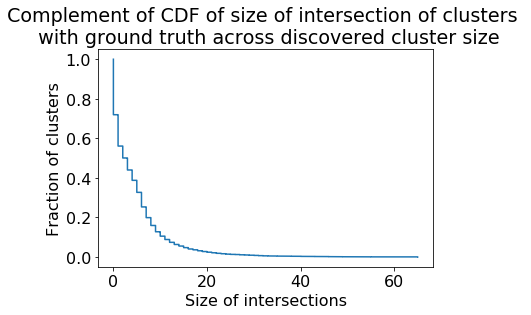
Figure 4: This figure looks as the quality of our extracted clusters compared with ground truth data. We compare results for the first 10000 communities extracted by our algorithm, and look at intersection size, excluding clusters with fewer than 5 vertices. We compare our clusters with the 5000 ‘high quality’ clusters from  [16].

For each set $X_{i}$, we find the ground truth community of highest Jaccard similarity with $X_{i}$. We plot the histogram of Jaccard similarities in  Fig. 4. We ignore clusters that have fewer than $5$ vertices for the purposes of this experiment; this accounts for only 42 of the total clusters extracted. For the remainder, we observe that the mean Jaccard density is 0.3, and 46 communities have a perfect value of 1. Moreover, we plot a similar histogram for size of intersection of our clusters with the ground truth. Here too we observe that the mean is 6.48. We look at how this average varies with sizes of the extracted clusters in  Fig. 5. While there is no clear trend observed in Jaccard density by cluster size, the mean intersection size clearly grows as we look at larger clusters.

Details of clusters:

A spectral triadic decomposition produces a large number of approximately uniform dense clusters, starting from only the promise of a large $\tau(G)$ value. In Fig. 7 and Fig. 8, we show a scatterplot of clusters, with axes of cluster size versus uniformity across various networks. We see that there are a large number of fairly large clusters (of size at least 20) and of uniformity at least 0.5; further discussion on the clusters and their sizes is in Tab. 3. These plots are further validation of the significance of Theorem 2.3 and the utility of the spectral triadic decomposition. The procedure Decompose automatically produces a large number of approximately uniform (or assortative) blocks in real-world networks. We summarize the data with some numbers in Tab. 2. We also plot the edge density and triangle density of these clusters, which are more standard parameters in network science. Refer to the first two rows of Fig. 6 respectively for these plots. Since edge density is at least the uniformity, as expected, we see a large number of dense clusters extracted by Decompose.

In Fig. 2, we show graph drawings of two example clusters in a co-authorship network of (over 90K) researchers in Condensed Matter Physics. The cluster on the left has $16$ vertices and $58$ edges, and has extracted a group of researchers who specialize in optics, ultra fast atoms, and Bose-Einstein condensates. Notable among them is the 2001 physics Nobel laureate Wolfgang Ketterle. The cluster on the right has $18$ vertices and $55$ edges, and has a group of researchers who all work on nanomaterials; there are multiple prominent researchers in this cluster, including the 1996 chemistry Nobel laureate Richard Smalley, who discovered buckminsterfullerene. We stress that the our decomposition found more than a thousand such clusters.

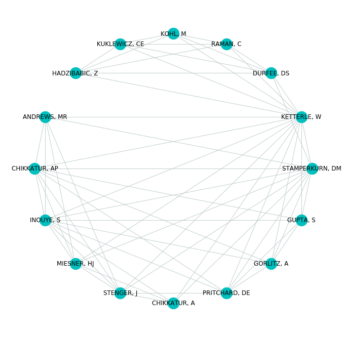
(a) Condensed Matter Physics: Cluster of researchers working on optics, ultra fast atoms, and Bose-Einstein condensates

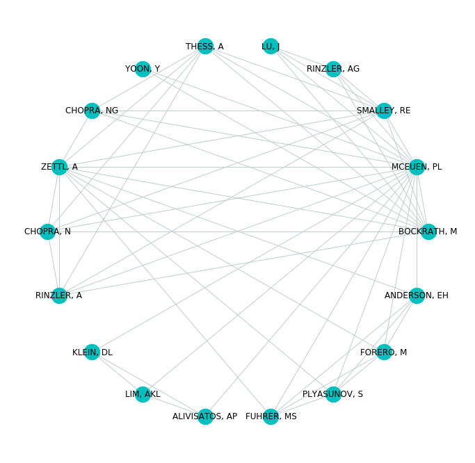
(b) Condensed Matter Physics: Cluster of researchers working on graphene, nanomaterials and topological insulators

Figure 2: We show two example clusters from a spectral triadic decomposition of coauthorship network of researchers in Condensed Matter Physics [9], a graph with $\tau=0.25$. The left cluster is a set of $16$ researchers ($58$ edges) working on optics and Bose-Einstein condensates (notably, the cluster has the 2001 Physics Nobel laureate Wolgang Ketterle). The right cluster has $18$ researchers ($55$ edges) working on nanomaterials, including the 1996 Chemistry Nobel laureate Richard Smalley.

Similar extracted clusters of research papers and articles extracted from the DBLP citation network can be seen in Fig. 3. In this case, one cluster is a group of papers on error correcting/detecting codes, while the other is a cluster of logic program and recursive queries papers.

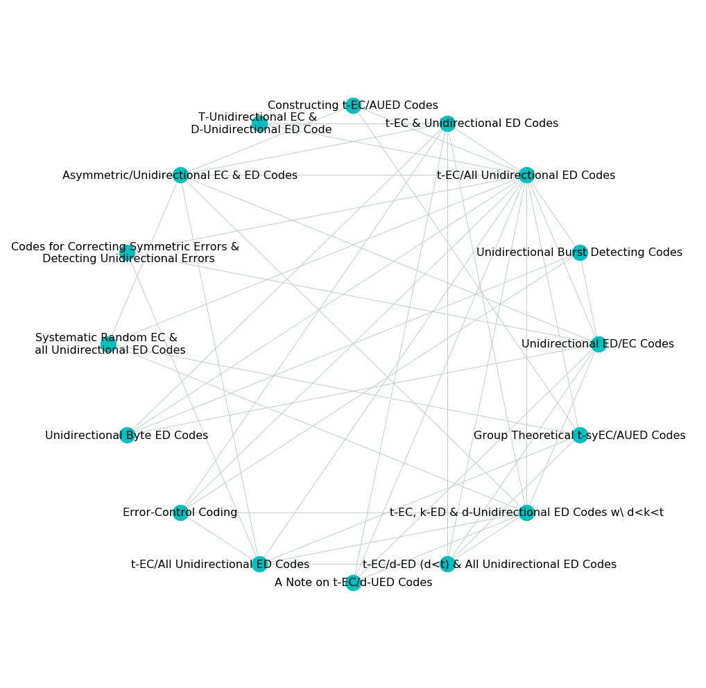
(a) DBLP: Cluster of papers on error correcting codes

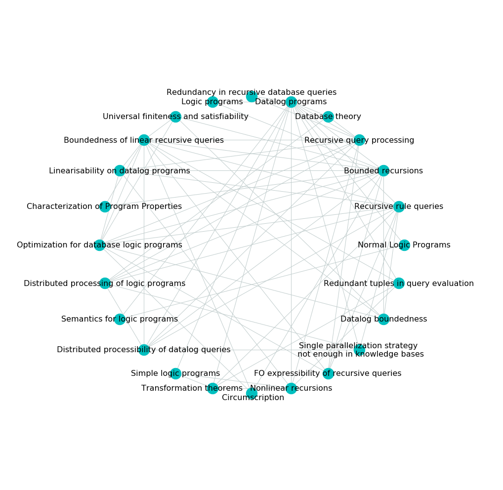
(b) DBLP: Cluster of papers on logic programs and recursive queries

Figure 3: We show example clusters from a spectral triadic decomposition of a DBLP citation network, involving papers in Computer Science  [16]. For ease of viewing, we label each vertex with relevant phrases from the paper title. The left cluster involves $16$ papers ($47$ edges) on the topic of error correcting codes. The right cluster of $24$ papers ($69$ edges) are all on the topic of logic programs and recursive queries, from database theory. Observe the tight synergy of topic among the vertices in a cluster; our procedure found thousands of such clusters.

It is surprising how well the spectral triadic decomposition finds fine-grained structure in networks, based on just the spectral transitivity. This aspect highlights the practical relevance of spectral theorems that decompose graphs into many blocks, rather that the classic Cheeger-type theorems that one produce two blocks.

Total content of decomposition:

Even though Decompose does not explicitly optimize for it, the clusters capture a large fraction of the vertices, and triangles. In Tab. 3, we see the latter values for all the decompositions constructed. A significant fraction of both vertices and the total triangle weight is preserved. Coverage is also impressive across the board; this is the total Frobenius norm of the decomposition, as a fraction of the total Frobenius norm of ${\cal A}$.. The cluster sizes vary with the dataset; the Facebook network shows especially large clusters; it also exhibits lower triangle weight retention, which may be an artefact of the fact that it is easier to retain triangle density in smaller clusters. A distribution of cluster sizes across datasets in shows in the histograms in the bottom row of Fig. 6.

Variation of $\varepsilon$:

The algorithm Decompose has only one parameter, $\varepsilon$, which determines the cleaning threshold. We vary the value of $\varepsilon$ from $0.1$ to $0.5$ on the network ca-HepTh. When $\varepsilon$ is smaller, the cleaning process removes fewer edges, but this comes at the cost of lower uniformity. For the mathematical analysis in §5, we require $\varepsilon$ to be smaller than $\tau$. On the other hand, the algorithm works in practice for large values of $\varepsilon$. The output of Decompose on fairly large values of $\varepsilon$ is quite meaningful.

We carry out the same experiments for four values of $\varepsilon$: $0.1,0.2,0.3,$ and $0.5$. The primary takeaway is that cleaning is far more aggressive for higher values of $\varepsilon$, and clusters extracted at higher values of are sparser. This is especially more pronounced for $\varepsilon=0.5$. We summarize the data and provide charts in a similar manner as before in Fig. 9, Fig. 10, Fig. 11 and Tab. 4.

7.2 Examination of Metadata Asssociated with Real Communities

In this last section, we look at a DBLP citation network from aminer.org: citation network V1  [12]. While the usual interpretation of a citation network is a a directed graph, we interpret it as an undirected graph with each directed edge in the graph corresponding to a corresponding undirected edge. While this dataset too gives us similar favorable statistics, the most compelling evidence provided by it is the corresponding metadata associated with the citation network. Given this, we evaluate it to see if the extracted clusters are semantically meaningful. This is strongly corroborated by the data: we exhibit an extracted cluster and the metadata associated to exhibit our case. Given that edges here are actual citations (agnostic to the direction), this shows that the internal density is an important metric to keep track of, as opposed to methods that find minimum edge cuts irrespective of what internal density of the components may look like. The results are listed in Tab. 5, Tab. 6, Tab. 7 and Tab. 8, where we lit the paper title, venue of publication, and the year of publication.

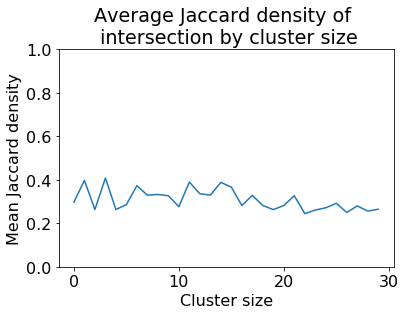
(a) Mean Jaccard density by cluster size

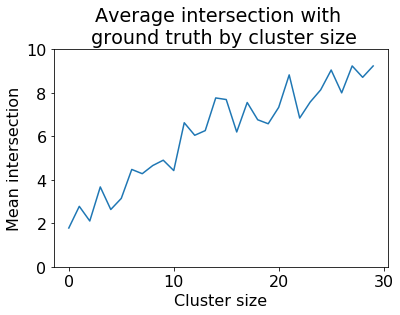
(b) Mean intersection by cluster size

Figure 5: Here we look at the mean values of Jaccard density and intersection size across clusters of different sizes. We compare results for the first 10000 communities extracted by our algorithm, and look at Jaccard density and intersection size, excluding clusters with fewer than 5 vertices. We compare our clusters with the 5000 ‘high quality’ clusters from  [16].

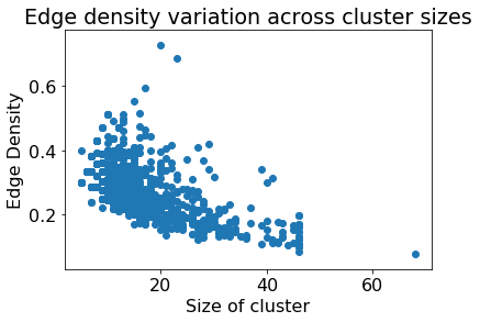
(a) ca-CondMat

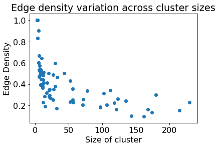
(b) socfb-Rice31

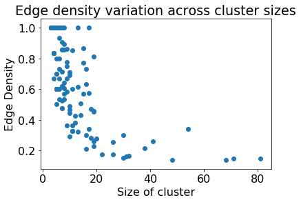
(c) soc-hamsterster

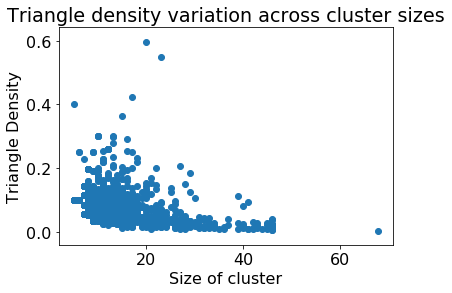
(d) ca-CondMat

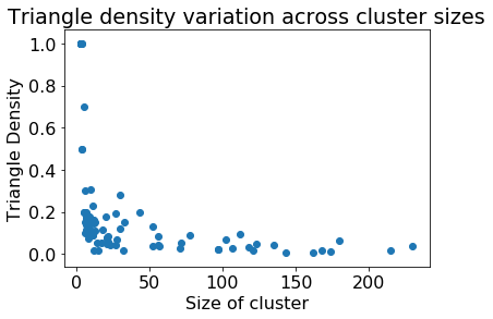
(e) socfb-Rice31

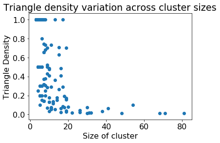
(f) soc-hamsterster

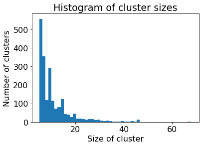
(g) ca-CondMat

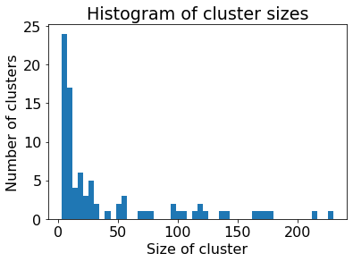
(h) socfb-Rice31

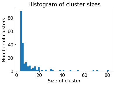
(i) soc-hamsterster

Figure 6: Scatter plot for edge density (top, (a)-(c)), triangle density (center, (d)-(f)) as a function of cluster size, and histogram of cluster sizes (bottom, (g)-(i)) for ca-CondMat, socfb-Rice31, and soc-hamsterster respectively, for $\varepsilon=0.1$.

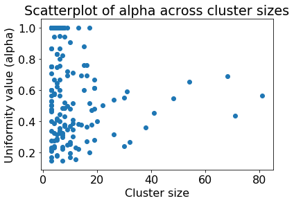
(a) Scatter plot for uniformity

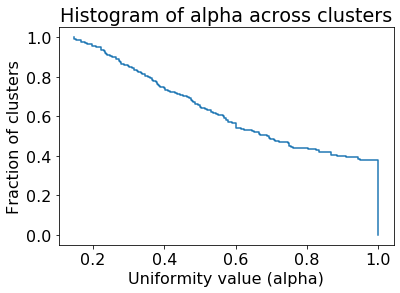
(b) Histogram for uniformity

soc-hamsterster

(c) Scatter plot for uniformity

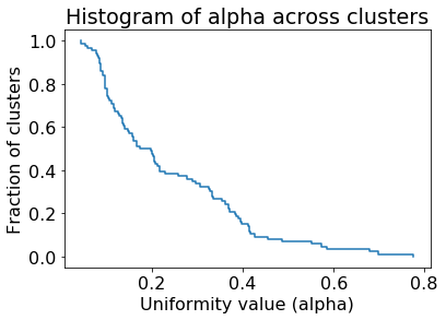
(d) Histogram for uniformity

socfb-Rice31

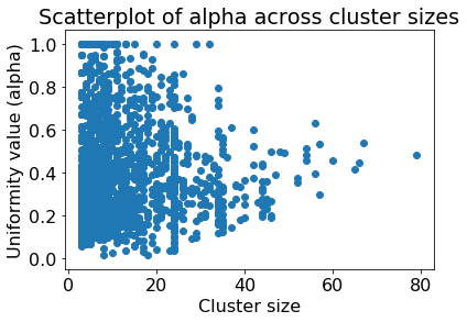
(e) Scatter plot for uniformity

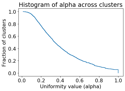
(f) Histogram for uniformity

cit-HepTh

Figure 7: A look at uniformity across clusters in the decomposition obtained from various networks as labelled. The figures on the left are straightforward scatter plots that looks at uniformity across clusters of varying sizes. Those on the right are complementary cumulative histograms for the uniformity values. The $x$-axis is the uniformity value, and the $y$ axis the fraction of clusters with at least that uniformity value.

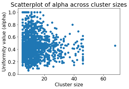
(a) Scatter plot for uniformity

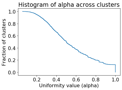
(b) Histogram for uniformity

ca-CondMat

(c) Scatter plot for uniformity

(d) Histogram for uniformity

ca-cond-matL

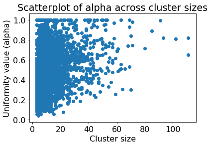
(e) Scatter plot for uniformity

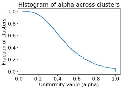
(f) Histogram for uniformity

cit-DBLP

Figure 8: (Continued)A look at uniformity across clusters in the decomposition obtained from various networks as labelled. The figures on the left are straightforward scatter plots that looks at uniformity across clusters of varying sizes. Those on the right are complementary cumulative histograms for the uniformity values. The $x$-axis is the uniformity value, and the $y$ axis the fraction of clusters with at least that uniformity value.

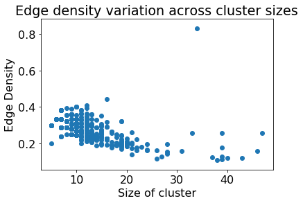
(a) $\varepsilon=0.1$

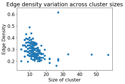
(b) $\varepsilon=0.2$

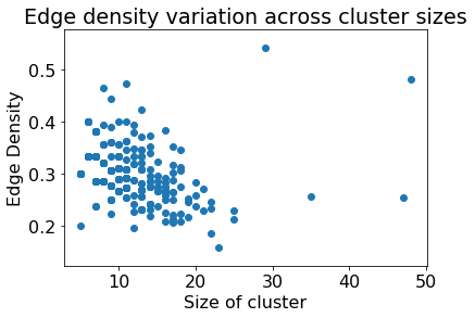
(c) $\varepsilon=0.3$

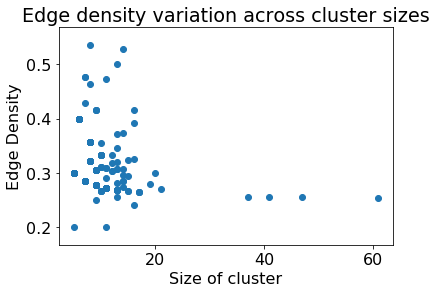
(d) $\varepsilon=0.5$

Figure 9: Scatter plot for edge density for ca-CondMat with varying values of $\varepsilon$.

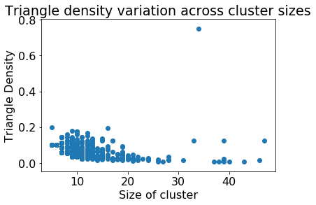
(a) $\varepsilon=0.1$

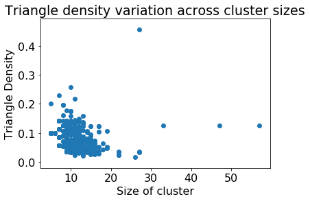
(b) $\varepsilon=0.2$

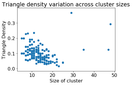
(c) $\varepsilon=0.3$

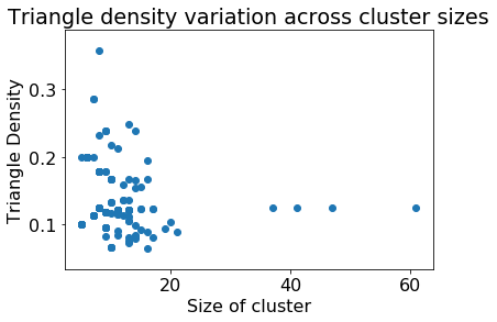
(d) $\varepsilon=0.5$

Figure 10: Scatter plot for triangle density for ca-CondMat with varying values of $\varepsilon$.

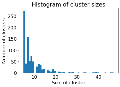
(a) $\varepsilon=0.1$

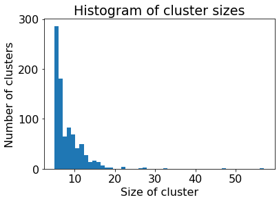
(b) $\varepsilon=0.2$

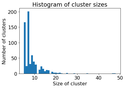
(c) $\varepsilon=0.3$

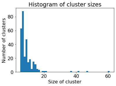
(d) $\varepsilon=0.5$

Figure 11: Histogram of cluster sizes for ca-CondMat with varying values of $\varepsilon$.

Dataset	#Vertices	#Edges	#Triangles	$\tau$
soc-hamsterster	2,427	16,630	53,251	0.215
socfb-Rice31	4,088	184,828	1,904,637	0.122
caHepTh	9,877	24,827	28,339	0.084
ca-cond-matL	16,264	47,594	68,040	0.255
ca-CondMat	23,133	93,497	176,063	0.125
cit-HepTh	27,770	352,807	1,480,565	0.122
cit-DBLP	217,312	632,542	248,004	0.087
ca-DBLP	317,080	1,049,866	2,224,385	0.248

Table 1: Summary of datasets used for different experiments. Most of our graphs are undirected, and the network names are indicative of what they are: names beginning with ‘ca’ refer to coauthorship networks (ca-CondMat is for researchers who work in condensed matter, ca-DBLP does the same for researchers whose work is on DBLP, a computer science bibliography website), ones beginning with ‘com’ are social networks (socfb-Rice31 is a Facebook network, soc-hamsterster is from Hamsterster, a pet social network), and ‘cit’ refers to citation networks. While citation networks are in reality directed graphs, we consider any directed edge to be an undirected edge for the purposes of our experiments. Graphs have been taken from the SNAP dataset at https://snap.stanford.edu/data/ [7] and the network repository at https://networkrepository.com/  [10]. The exceptions to this are the cit-DBLP dataset, which has been taken from https://www.aminer.org/citation [12] and the ca-cond-matL dataset, which has been taken from  [9] ; the L is for labelled. For cit-DBLP, the $\tau$ value is for the $2$-core of the graph.

Dataset	Mean Uniformity	10th percentile	Min uniformity
soc-hamsterter	0.68	0.26	0.15
socfb-Rice31	0.24	0.08	0.04
ca-HepTh	0.61	0.31	0.12
ca-CondMat	0.55	0.25	0.06
ca-cond-matL	0.86	0.57	0.27
cit-HepTh	0.41	0.14	0.01
cit-DBLP	0.50	0.24	0.04
ca-DBLP	0.67	0.33	0.07

Table 2: Summary of data about the extracted clusters across datasets: number of clusters, percentage of total number of vertices preserved in clusters, total triangle weight preserved in clusters, minimum of cluster sizes, maximum of cluster sizes, average of cluster sizes when $\varepsilon-0.1$..

Dataset	#Clusters	% Vtx	% Tri-Wt	Coverage %	Cluster Sizes
					Min	Max	Avg
soc-hamsterster	208	76.09	80.94	85.34	3	81	8.88
socfb-Rice31	86	86.84	24.71	36.76	3	230	41.27
ca-HepTh	849	77.46	71.43	73.79	5	47	9.01
ca-CondMat	2049	95.45	71.61	58.84	5	68	10.78
ca-condmatL	1566	75.57	77.90	78.64	3	47	7.85
cit-HepTh	1664	73.74	53.81	58.84	3	79	12.31
cit-DBLP	7265	27.57	70.04	77.15	3	111	8.25

Table 3: Summary of data about the extracted clusters across datasets: number of clusters, percentage of total number of vertices preserved in clusters, total triangle weight preserved in clusters, coverage, and cluster sizes (minimum, maximum and average). We observe great diversity in the nature of clusters extracted; most datasets have average cluster sizes between $7$ and $13$, with the exception of socfb-Rice31, where the average is as high as $41$. Number of vertices preserved is consistently high except for the cit-DBLP network, which had remarkably low edge and triangle density to begin with. Triangle weight preserved and coverage are also remarkably high across all datasets; albeit a bit lower in socfb=Rice31.

$\varepsilon$	#Clusters	% Vtx	% Tri-Wt	Cluster Min	Cluster Max	Cluster Avg
0.1	849	11.13	58.63	5	47	9.01
0.2	866	10.56	59.04	5	57	8.39
0.3	652	8.08	54.99	5	48	8.52
0.5	296	3.85	36.00	5	61	8.95

Table 4: Summary of data about the extracted clusters on caHepTh for $\varepsilon\in\{0.1,0.2,0.3,0.5\}$: number of clusters, percentage of total number of vertices preserved in clusters, total triangle weight preserved in clusters, minimum of cluster sizes, maximum of cluster sizes, average of cluster sizes.

Paper Title	Venue	Year
Some comments on the aims of MIRFAC	Communications of the ACM	1964
MIRFAC: a compiler based on standard mathematical notation and plain English	Communications of the ACM	1963
MIRFAC: a reply to Professor Djikstra	Communications of the ACM	1964
More on reducing truncation errors	Communications of the ACM	1964
The dangling else	Communications of the ACM	1964
MADCAP: a scientific compiler for a displayed formula textbook language	Communications of the ACM	1961
Further comment on the MIRFAC controversy	Communications of the ACM	1964
An experiment in a user-oriented computer system	Communications of the ACM	1964
Automatic programming and compilers II: The COLASL automatic encoding system	Proceedings of the 1962 ACM national conference on Digest of technical papers	1962

Table 5: Metadata for cluster extracted from cit-DBLP: Cluster of size 9, edge density of 0.472

Paper Title	Venue	Year
Measurement-based characterization of IP VPNs	IEEE/ACM Transactions on Networking (TON)	2007
Traffic matrices: balancing measurements, inference and modeling	Proceedings of the 2005 ACM SIGMETRICS international conference on Measurement and modeling of computer systems	2005
Data streaming algorithms for accurate and efficient measurement of traffic and flow matrices	ACM SIGMETRICS Performance Evaluation Review	2005
An information-theoretic approach to traffic matrix estimation	Proceedings of the 2003 conference on Applications, technologies, architectures, and protocols for computer communications	2003
Atomic Decomposition by Basis Pursuit	SIAM Review	2001
Solving Ill-Conditioned and Singular Linear Systems: A Tutorial on Regularization	SIAM review	1998
Structural analysis of network traffic flows	ACM Sigmetrics performance evaluation review	2004
How to identify and estimate the largest traffic matrix elements in a dynamic environment	Proceedings of the joint international conference on Measurement and modeling of computer systems	2004
Relative information: theories and applications	Book	1990
Estimating point-to-point and point-to-multipoint traffic matrices: an information-theoretic approach	IEEE/ACM Transactions on Networking (TON)	2005
Traffic matrix tracking using Kalman filters	ACM Sigmetrics performance evaluation review	2005
Towards a meaningful MRA of traffic matrices	Proceedings of the 8th ACM SIGCOMM conference on Internet measurement	2008

Table 6: Metadata for cluster extracted from cit-DBLP: Cluster of size 12, edge density of 0.83

Paper Title	Venue	Year
A Cell ID Assignment Scheme and Its Applications	Proceedings of the 2000 International Workshop on Parallel Processing	2000
High-Performance Computing on a Honeycomb Architecture	Proceedings of the Second International ACPC Conference on Parallel Computation	1993
Optimal dynamic mobility management for PCS networks	IEEE/ACM Transactions on Networking (TON)	2000
Higher dimensional hexagonal networks	Journal of Parallel and Distributed Computing	2003
Addressing and Routing in Hexagonal Networks with Applications for Tracking Mobile Users and Connection Rerouting in Cellular Networks	IEEE Transactions on Parallel and Distributed Computing	2002
Addressing, Routing, and Broadcasting in Hexagonal Mesh Multiprocessors	IEEE Transactions on Computers	1990
Performance Analysis of Virtual Cut-Through Switching in HARTS: A Hexagonal Mesh Multicomputer	IEEE Transactions on Computers	1990
HARTS: A Distributed Real-Time Architecture	Computer	1991
Cell identification codes for tracking mobile users	Wireless Networks	2002

Table 7: Metadata for cluster extracted from cit-DBLP: Cluster of size 9, edge density of 0.33

Paper Title	Venue	Year
Classical linear logic of implications	Mathematical Structures in Computer Science	2005
Logic continuations	Journal of Logic Programming	1987
Axioms for control operators in the CPS hierarchy	Higher-Order and Symbolic Computation	2007
Formalizing Implementation Strategies for First-Class Continuations	Proceedings of the 9th European Symposium on Programming Languages and Systems	2000
Linearly Used Effects: Monadic and CPS Transformations into the Linear Lambda Calculus	Proceedings of the 6th International Symposium on Functional and Logic Programming	2002
On Exceptions Versus Continuations in the Presence of State	Proceedings of the 9th European Symposium on Programming Languages and Systems	2000
What is a Categorical Model of Intuitionistic Linear Logic?	Proceedings of the Second International Conference on Typed Lambda Calculi and Applications	1995
Using a Continuation Twice and Its Implications for the Expressive Power of call/cc	Higher-Order and Symbolic Computation	1999
From control effects to typed continuation passing	Proceedings of the 30th ACM SIGPLAN-SIGACT symposium on Principles of programming languages	2003
Continuations: A Mathematical Semantics for Handling FullJumps	Higher-Order and Symbolic Computation	2000
Comparing Control Constructs by Double-Barrelled CPS	Higher-Order and Symbolic Computation	2002
Linear Continuation-Passing	Higher-Order and Symbolic Computation	2002
Definitional Interpreters for Higher-Order Programming Languages	Higher-Order and Symbolic Computation	1998
Essentials of programming languages	Book	1992
Glueing and orthogonality for models of linear logic	Theoretical Computer Science	2003
Frame rules from answer types for code pointers	Conference record of the 33rd ACM SIGPLAN-SIGACT symposium on Principles of programming languages	2006

Table 8: Metadata for cluster extracted from cit-DBLP: Cluster of size 16, edge density of 0.42

References

- [1] A. Barrat, M. Barthélemy, R. Pastor-Satorras, and A. Vespignani. The architecture of complex weighted networks. Proceedings of the National Academy of Sciences, 101(11):3474–3452, 2004.
- [2] M. Granovetter. The strength of weak ties: A network theory revisited. Sociological Theory, 1:201–233, 1983.
- [3] Rishi Gupta, Tim Roughgarden, and C. Seshadhri. Decompositions of triangle-dense graphs. Innovations in Theoretical Computer Science, pages 471–482, 2014.
- [4] J. Kleinberg. Navigation in a small world. Nature, 406(6798), 2000.
- [5] James R. Lee, Shayan Oveis Gharan, and Luca Trevisan. Multiway spectral partitioning and higher-order cheeger inequalities. J. ACM, 61(6):1–30, 2014.
- [6] J. Leskovec, K. J. Lang, A. Dasgupta, and M. W. Mahoney. Community structure in large networks: Natural cluster sizes and the absence of large well-defined clusters. Internet Mathematics, 6(1):29–123, 2009.
- [7] Jure Leskovec and Andrej Krevl. SNAP Datasets: Stanford large network dataset collection. http://snap.stanford.edu/data, June 2014.
- [8] S. Milgram. The small world problem. Psychology Today, 1(1):60–67, 1967.
- [9] M. E. J. Newman. The structure of scientific collaboration networks. Proceedings of the National Academy of Sciences, 98(2):404–409, 2001.
- [10] Ryan A. Rossi and Nesreen K. Ahmed. The network data repository with interactive graph analytics and visualization. AAAI, 2015.
- [11] C. Seshadhri, Tamara G. Kolda, and Ali Pinar. Community structure and scale-free collections of Erdos-Renyi graphs. Physical Review E, 85:056109, 2012.
- [12] Jie Tang, Jing Zhang, Limin Yao, Juanzi Li, Li Zhang, and Zhong Su. Arnetminer: Extraction and mining of academic social networks. SIGKDD Conference on Knowledge Discovery and Data Mining (KDD), page 990–998, 2008.
- [13] Amanda L Traud, Eric D Kelsic, Peter J Mucha, and Mason A Porter. Comparing community structure to characteristics in online collegiate social networks. SIAM Rev., 53(3):526–543, 2011.
- [14] Amanda L Traud, Peter J Mucha, and Mason A Porter. Social structure of Facebook networks. Phys. A, 391(16):4165–4180, Aug 2012.
- [15] S. Wasserman and K. Faust. Social Network Analysis: Methods and Applications. Cambridge University Press, 1994.
- [16] Jaewon Yang and Jure Leskovec. Defining and evaluating network communities based on ground-truth. CoRR, abs/1205.6233, 2012.