DistGNN-MB: Distributed Large-Scale Graph Neural Network Training on x86 via Minibatch Sampling

Abstract.

Training Graph Neural Networks, on graphs containing billions of vertices and edges, at scale using minibatch sampling poses a key challenge: strong-scaling graphs and training examples results in lower compute and higher communication volume and potential performance loss. DistGNN-MB employs a novel Historical Embedding Cache combined with compute-communication overlap to address this challenge. On a $32$-node ($64$-socket) cluster of 3rd generation Intel®  Xeon®  Scalable Processors with 36 cores per socket, DistGNN-MB trains $3$-layer GraphSAGE and GAT models on OGBN-Papers100M to convergence with epoch times of $2$ seconds and $4.9$ seconds, respectively, on $32$ compute nodes. At this scale, DistGNN-MB trains GraphSAGE $5.2\times$ faster than the widely-used DistDGL. DistGNN-MB trains GraphSAGE and GAT $10\times$ and $17.2\times$ faster, respectively, as compute nodes scale from $2$ to $32$.

1. Introduction

Graph Neural Networks (GNN) are fast becoming a mainstream technology ingredient in applications such as recommendation systems (Ying et al., 2018), fraud detection (Liu et al., 2021), and large-scale drug discovery (Zitnik et al., 2018). Interestingly, unlike Deep Learning techniques in vision or language modeling, GNN-based learning must adapt to the size and types of graphs whose structure the model must learn. Thus, for some applications, e.g., fraud detection, training the model on the full graph (aka full-batch training) will likely deliver better accuracy than sampling-based minibatch training, whereas for applications such as recommendation systems the latter is likely to be more scalable and accurate (Ying et al., 2018) . Additionally, the class of applications devoted to molecule search and discovery involves millions of "small" graphs each with only a few hundred or thousand vertices, requiring a combination of techniques employed in both full-graph and minibatch training to achieve good performance and high accuracy. This paper focuses on the performance of distributed, large-scale minibatch GNN training on CPUs.

In general, GNN training involves recursively executing (to the chosen depth) two key steps or primitives in order on chosen training examples: Aggregation (AGG) and UPDATE. In AGG, source vertex or edge features are aggregated to destination vertices in the graph via message passing along the edges. In UPDATE, aggregated features pass through a Multi-Layer Perceptron (MLP). Typical downstream tasks for a trained GNN model include node- (i.e., vertex), link- and graph-property prediction. Thus, the last hop of the AGG-UPDATE sequence consists of a classifier function to output predictions. A loss function, such as Cross-Entropy Loss or Negative-Log Likelihood compute the loss with respect to the target and errors backpropagate through UPDATE-AGG sequences.

Minibatch GNN training Similar to domains such as vision or language modeling, a GNN model uses a sampled minibatch of examples as inputs to execute AGG-UPDATE sequences for training. Unlike vision or language modeling, however, minibatch construction is more complex. GNN training examples are a set of vertices; each iteration constructs a minibatch of sub-graphs with a subset of the training vertices as roots. Each sub-graph is formed by recursively sampling a fixed number of neighbors starting from root vertices to the desired depth. Sampling can be uniform, biased or importance-based. The cost of minibatch creation can become a dominant component of overall training time; cost mitigation solutions include parallelization and asynchronous execution to overlap minibatch creation with compute. As discussed earlier, the UPDATE primitive in GNN training typically consists of an MLP, which in turn, consists of a matrix-matrix multiplication (matmul) operation followed by a non-linear function (e.g., ReLU or sigmoid) and a regularization function (e.g., Dropout). While matmul is compute-intensive operation, ReLU and Dropout are memory-bandwidth intensive. Thus, the challenge is to ensure that these operations execute efficiently both with respect to the available compute power of the CPU as well as memory bandwidth.

Distributed GNN Training GNNs naturally exhibit data parallelism because they are constructed either on instances of a single large graph (with billions of vertices and edges) or millions of small graphs (with only a few thousand vertices and edges). In the case of large-graphs, training GNN models requires partitioning them into smaller sub-graphs, and assigning each sub-graph to a CPU; it also requires splitting training example vertices in a balanced manner into the specified number of parts. Minimum-cut algorithms can partition such graphs along vertices (Xie et al., 2014) or edges (Karypis and Kumar, 1997; Karypis et al., 1997) into a specified number of sub-graphs. In the case of millions of small graphs (e.g., molecule graphs) training GNN models is an embarrassingly parallel problem, as each node in a cluster can feed a batch of example graphs in parallel to the model.

Challenges of distributed, minibatch GNN training Because we focus on training performance of large-scale GNNs in a distributed minibatch setting across CPUs via graph partitioning, we consider the following. As a result of splitting training examples into smaller parts, with each part is assigned to a single CPU socket, the number of minibatches per socket reduces. Thus, not only does each CPU socket train the GNN model using a graph partition, but also samples fewer minibatches compared to single-CPU training. As a result of graph partitioning, AGG now has two components: local and remote. The performance problem is now clear: as we partition graphs into smaller sub-graphs, each CPU socket uses fewer sub-graphs to train the model, and communication between CPU sockets to compute remote AGG increases and begins to dominate at scale. The accuracy problem is that the size of the minibatch per socket remains the same; thus, the global minibatch scales with the number of CPU sockets potentially affecting accuracy. Thus, the constraint on improving performance via scaling is to achieve the same (or within some $\epsilon$ of) target accuracy as single CPU training.

Contributions This paper addresses these challenges and makes the following contributions:

• A novel compute-communication overlap algorithm to reduce communication overhead at scale

• A novel, software-managed Historical Embedding Cache (HEC) data structure and associated algorithm that reduces communication without impacting accuracy

• Performance-optimized minibatch creation algorithm on CPUs to reduce overhead at scale

• Performance-optimized UPDATE primitive on CPUs to ensure efficient execution

• Demonstrating large-scale GNN minibatch training using the open-source, widely-used Deep Graph Library (DGL) on general-purpose, CPU-only clusters with high performance

The rest of the paper is organized as follows: Section 2 discusses GNN preliminaries along with the GraphSAGE (Hamilton et al., 2017) and Graph Attention Network (GAT) (Veličković et al., 2018) models. In section 3, we detail our Asynchronous Embedding Push AEP algorithm which uses HEC, along with performance optimizations to minibatch sampling, AGG and UPDATE primitives. Section 4 presents and discusses performance and accuracy evaluation results in detail. In section 5 we briefly describe related research in large-scale GNN minibatch training. We present concluding remarks and discuss future work in section 6.

2. Background

Given an input graph $\mathcal{G}(\mathcal{V},\mathcal{E}),(v,\mathcal{N}(v))\in\mathcal{V}$ (where $\mathcal{N}$($v$) is the neighborhood of $v$), and an $\mathcal{L}$-layer GNN constructed on $\mathcal{G}$, GraphSAGE (shown in equation 1) performs AGG and UPDATE for each layer $l$ on vertex features $f^{l}$. In distributed training, $\mathcal{N}(v)$ may reside on the local CPU or on a remote CPU. Thus, AGG is executed as local and remote (section 3.2) operations, with the latter resulting in the need for communications. GraphSAGE consists of two matmul operations: one transforms neighbor aggregates ${h^{l}}_{\mathcal{N}(v)}$ using model parameters ${W^{l}}_{n}$ (where $n$ denotes "neighborhood") and the other transforms the vertex’s own features ${h^{l}}_{v}$ using model parameters ${W^{l}}_{s}$ (where $s$ denotes "self"). GraphSAGE uses ReLU to non-linearize embeddings and Dropout to generate the final, regularized output ${h^{l}}_{v}$ for layer $l$. In distributed training, CPUs perform all-reduce communication to exchange model parameter gradients and update model parameters locally.

(1) $$\begin{split}&{h^{l}}_{\mathcal{N}(v)}={\tt AGG}{}^{l}(\left\{f^{l-1}_{u}|u\in\mathcal{N}(v)\right\})\\ &{h^{l}}_{v}={\tt Dropout}({\tt ReLU}({W^{l}}_{n}\cdot{h^{l}}_{\mathcal{N}(v)}+{W^{l}}_{s}\cdot{h^{l}}_{v}+b^{l})\end{split}$$

Similarly, on an input graph $\mathcal{G}$ and a $\mathcal{L}$-layer GNN, the GAT model (shown in equation 2) performs AGG and UPDATE for each layer $l$ on vertex features. In this work, we modify DGL’s implementation of GAT to enable performance optimizations; we have empirically determined that these modifications do not materially impact accuracy. Our modification applies bias and non-linearity to the output of dot-product between embeddings and model parameters before computing attention co-efficients ${\alpha^{l}}_{uv}$. The dot-product, edge-feature and attention-coefficient computation operations execute locally on each machine. AGG executes in a distributed manner as described above.

(2) $$\begin{split}&{z^{l}}_{u}={\tt ReLU}({W^{l}}_{u}\cdot{f^{l}}_{u}+{b^{l}})\\ &{z^{l}}_{v}={\tt ReLU}({W^{l}}_{v}\cdot{f^{l}}_{v}+{b^{l}})\\ &{e^{l}}_{u}={W^{l}}_{au}\circ{z^{l}}_{u}\\ &{e^{l}}_{v}={W^{l}}_{av}\circ{z^{l}}_{v}\\ &{\alpha^{l}}_{uv}={\tt EdgeSoftmax}({\tt LeakyRELU}({e^{l}}_{u}+{e^{l}}_{v}))\\ &{h^{l+1}}_{v}={\tt AGG}{}^{l}({{\alpha}^{l}}_{uv}{z^{l}}_{u}|u\in\mathcal{N}(v)))\end{split}$$

3. Distributed Minibatch Training

GNN training is demanding in terms of compute resources, i.e., CPUs, memory capacity and memory bandwidth. Training massive graphs on a single CPU socket is challenging due to such resource requirements. AGG is a memory-intensive operation, with a byte-to-op ratio $\gg 1$; e.g., aggregating two $256$-element FP$32$ tensors with $+$ operator requires $3072$ bytes to be Read/Written, with only $256$ compute operations – a byte-to-op ratio of $12$. Thus, using naive AGG and UPDATE implementations for large-scale GNN training on a single CPU socket will result in poor performance.

In this section, we discuss algorithms for distributed, large-scale minibatch GNN training including important single-socket CPU optimizations; these algorithms and optimizations enable DisGNN-MB to achieve at least an order-of-magnitude speedup over naive single-socket CPU implementations.

The key to GNN model training in a distributed environment is partitioning the underlying graph into smaller sub-graphs (section 3.1). Because AGG contains a reduction operator, graph partitioning will automatically result in feature vector (or vertex embedding) communication to ensure correct and complete the AGG operation. To reduce communication overhead, the graph partitioning algorithm usually cuts minimum number of edges or vertices while creating partitions with balanced training examples. In this work, we use a modified version of the popular algorithm, Metis, which employs a minimum-edge-cut technique to partition graphs.

However, while balanced min-edge-cut partitioning is necessary for communication-reduction, it is not sufficient to hide communication-cost. An un-optimized AGG implementation may potentially create a large performance bottleneck by communicating vertex embeddings for every layer in each minibatch, if these communications cannot be overlapped with compute. Common techniques to mitigate this problem fall into two broad approaches: communication volume reduction per iteration and avoidance across iterations.

In this paper, we describe a suite of algorithms and a data structure called HEC for volume reduction via communication delay; to further reduce overall cost, we overlap communications with local compute on every CPU socket in the distributed system. (For ease of usage, we refer to CPU sockets in a distributed system as ranks in the rest of the paper.)

3.1. Metis Graph Partitioning with Balance

In addition to minimal edge-cuts, GNNs have a specific requirement: training vertices must be distributed among graph partitions to minimize load imbalance across ranks. DistDGL (Zheng et al., 2020) augments Metis meet this requirement. We define key terms required to denote various entities as a result of min-edge-cut partitioning: solid and halo vertices, original (${\tt VID}{}_{o}$), partition (${\tt VID}{}_{p}$) and batch vertex IDs (${\tt VID}{}_{b}$), respectively.

Let an edge $e=(u,v)$ in the full graph $\mathcal{G}$ be a min-cut edge during partitioning. Thus, $e$ is cut into two edges ${e^{\prime}}=(u,v^{\prime})$ and $e^{\prime\prime}=(u^{\prime},v)$. We refer to $u^{\prime}$ and $v^{\prime}$ as halo vertices, which represent their corresponding solid vertices $u$ and $v$ in the other partition, respectively. Halo vertices $u^{\prime}$ and $v^{\prime}$ do not contain input features. During AGG, solid vertices $u$ and $v$ communicate embeddings to $u^{\prime}$ and $v^{\prime}$, respectively; these embeddings are aggregated with their corresponding destination vertices via message passing within their respective partitions. Per definition of $\mathcal{G}$, ${\tt VID}{}_{o}=range(0...\mathcal{V}-1)$. Let the number of vertices in a partition be $\mathcal{P}$; then ${\tt VID}{}_{p}=range(0...\mathcal{P}-1)$. Finally, let the number of vertices in a minibatch be $\mathcal{B}$; then ${\tt VID}{}_{b}=range(0...\mathcal{B}-1)$. DistGNN-MB uses lookup tables to maintain correspondence between ${\tt VID}{}_{o}$, ${\tt VID}{}_{p}$, and ${\tt VID}{}_{b}$.

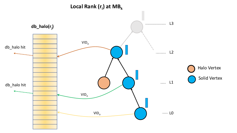
(a)

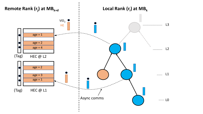
(b)

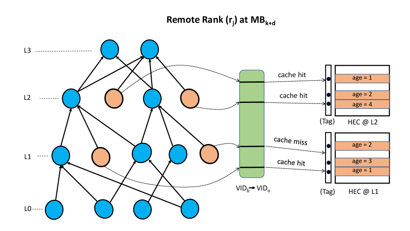
(c)

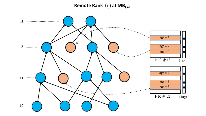
(d)

Figure 1. $n$ layers in minibatch (MB) are labelled as L₀, L₁ …L_n-1, with L_n-1 containing training seed vertices. Minibatch contains solid and halo vertices. Solid-vertex embeddings communication is asynchronous, with delay $d$, to fill remote HECs. Halo-vertex search occurs in local HEC and corresponding embeddings are used during MB AGG. Each inner MB layer maintains an HEC. (a) Each remote rank $r_{j}$ searches for solid vertices of local MB in db_halo; embdeddings of vertices with db_halo hit become eligible for communication to remote HECs. (b) rank $r_{i}$, processing $k^{th}$ minibatch, MB_k, asynchronously communicates the selected solid vertices (${\tt VID}{}_{o}$) and their embeddings to HEC of remote rank $r_{j}$; $r_{j}$ receives the communication while processing of $(k+d)^{th}$ minibatch, MB_k+d, overlapping communication with computation of $d$ minibatches. Received embeddings are cached in local HEC with $age$ set for the occupied cache-lines. (c) Before performing AGG, rank $r_{j}$ searches for its halo vertices in local HEC. Accessing local HEC requires conversion from ${\tt VID}{}_{b}$ to ${\tt VID}{}_{o}$ as ${\tt VID}{}_{o}$ are maintained as HEC tags. (d) Embeddings for halo vertices with a cache-hit are loaded from HEC during AGG.

3.2. Remote Aggregation using Delayed, Historical Embeddings

Local aggregation executes as shown in equations 1 and  2 in section 2. In this section, we focus exclusively on optimized remote aggregation to reduce communication cost.

To accomplish remote aggregation, we employ the Historical Embedding (HE) concept. As (Chen et al., 2017) describe, HEs are embeddings from past training iterations, which under conditions of bounded staleness (Fey et al., 2021), (Peng et al., 2022) contribute usefully to model convergence (and more importantly, do not degrade accuracy). The key advantage of HE in GNN training is in saving embedding communication time by using a locally available, albeit stale version to complete the AGG step. To improve HE utility and reuse, we introduce HEC, a software-managed cache containing HE as cache-lines. Each rank in the distributed system creates and associates an HEC with each GNN layer. HEC has a fixed size $cs$ and each cache-line has a maximum life-span $ls$; all cache-lines with age greater than $ls$ are purged from HEC. ${\tt VID}{}_{o}$ serve as tags to quickly find and access cache-lines in HEC. Cache-line replacement in HEC follows oldest cache-line first (OCF) policy. This ensures fresher embeddings in the HEC.

HEC plays a key role in ensuring compute-communication overlap during remote aggregation by serving as a repository for delayed embeddings, as shown in figure 1(b); e.g., a local rank generates an embedding HE at MB_k that a remote rank receives at MB_k+d, after a delay of $d$ iterations, which HEC stores (either by replacing an existing cache-line with a matching tag, replacing an expired cache-line or filling a new cache line entry). An additional benefit of HEC is that unlike DistDGL, ranks do not need to prefetch vertices from remote neighbors after minibatch creation to determine connectivity at run-time and establish "remote edges" for message passing; they merely reuse cached HE via ${\tt VID}{}_{o}$ tags received and stored as part of communication processing.

HEC management consists of three key operations: HECSearch, HECLoad and HECStore. For each halo vertex $hv$, HECSearch searches HEC efficiently for resident HE $f_{hv}$ using ${\tt VID}{}_{o}$ as the corresponding tag and returns a pointer to the matching line on a hit. HECLoad gathers embeddings $f$ using memory pointers (that HECSearch returns) and stores them into the minibatch data structure for AGG. HECStore scatters embeddings received from remote partitions via asynchronous communication into the HEC. We have optimized these management functions to perform lookup, gather and scatter operations efficiently using OpenMP® parallel regions.

One of the most important data structures in DistGNN-MB is db_halo. On each rank in the distributed system, it stores original vertex IDs ${\tt VID}{}_{o}$ associated with halo vertices from remote partitions (whose solid avatars exist local partition). Each minibatch sampled locally contains both solid and halo vertices. Using mappings in db_halo, our optimized communication algorithm retrieves features/embeddings required by remote halo vertices ${\tt VID}{}_{o}$ and asynchronously communicates them to remote partitions. The Map function to map solid to halo vertices during minibatch training is one of the most expensive operations in DistGNN-MB and we optimize it using OpenMP® parallel regions.

The graph partition data-structure that Metis creates is also very important. It maintains details about each graph vertex in a lookup table (LUT). These details include markers to identify vertex type (solid or halo) and ${\tt VID}{}_{o}$. In DGL, the minibatch creation process provides the LUT to map minibatch vertex IDs ${\tt VID}{}_{b}$ to partition IDs ${\tt VID}{}_{p}$. Partition IDs can be used to index into the graph LUT to identify the corresponding vertex type (findHaloNodes() and findSolidNodes() in Algorithm 2) and original vertex IDs ${\tt VID}{}_{o}$ (for HEC access and communication). We optimize these functions also using OpenMP parallel regions.

3.2.1. Asynchronous Embedding Push (AEP) Algorithm

We apply the AEP algorithm to fill HEC with historical embeddings, optimize remote aggregation and reduce communication overhead during distributed minibatch GNN training. At each GNN layer, AEP pushes solid-vertex embeddings from the current local minibatch to remote HECs, asynchronously. AEP overlaps communication across iterations, with minibatch computation and communication-data-structure management functions. Remote HECs fill with HE cache-lines in preparation for their use in subsequent local minibatches.

In line $2$ of Algorithm 2, all ranks initialize their HEC (as described in Algorithm 1), at each GNN layer with parameters $cs$, $nc$ and $ls$ described earlier. Additionally, each rank is assigned a graph partition $P$. Each rank creates its db_halo database using remote partition $hv$, as shown in Algorithm 1.

Lines $3$-$27$ run for a configurable number of epochs. After creating minibatches (MB) and extracting seeds on Line $4$, the algorithm iterates through all $M$ minibatches on Line $5$. Line $6$ gathers minibatch features using seeds as indices.

On Lines $7$-$13$, each rank does the following: On Line $8$, it determines whether to wait for communication of delayed remote partition halo vertices ($h_{v}$) and corresponding embeddings ($f_{hv}$) (figure 1(b)). If so, and upon receipt, each rank stores $f_{hv}$ into its HEC on Line $9$. On Lines $10$-$11$ (figure 1(c)), each rank extracts minibatch halo vertices and uses them to search through its HEC for embeddings. It combines them with minibatch embeddings ($f_{mb}$) (figure 1(d)). On Line $11$, a rank may encounter a cache miss in its HEC – if so, it eliminates the corresponding $hv$ from minibatch execution. Now, AGG in equations 1 and 2 can execute on $f_{mb}$, thus completing the overall AGG operation. As part of training, this is followed by UPDATE.

Each rank executes Lines $15$-$24$ to asynchronously communicate solid-vertex embeddings to remote ranks if minibatch iteration $k$ is within $M-d$ iterations. On Line $15$, each rank extracts its minibatch solid vertices and uses them to retrieve a subset $sv^{\prime}$ from db_halo (Line 18) as shown in figure 1(a). Each rank restricts the number of retrieved solid vertices to a configurable parameter $nc$; it does this by randomly sampling a subset of $sv^{\prime}$ based on their degree (Line 20). On Line 22, each rank gathers features ($f_{sv^{\prime}}$) associated with $sv^{\prime}$ locally. Finally, on Line 24, all ranks send $f_{sv^{\prime}}$ to remote ranks (figure 1(b)). Execution repeats on Line 8 and continues until all epochs have completed.

Algorithm 1 Initialize

0:  Graph partition $P$

0:  HEC

0:  HEC parameters: $cs$, $nc$, $ls$

0:  Partition halo vertices, $hv$

1:  Assign $P$ to a rank

2:  $B$ $\leftarrow$ Bcast($hv$)

3:  db_halo $\leftarrow{}$ CreateDB($B$)

4:  ${\tt HEC}{}$.cs = cs

5:  ${\tt HEC}{}$.nc = nc

6:  ${\tt HEC}{}$.ls = ls

Algorithm 2 Asynchronous Embedding Push

0:  Per partition vertex features, $f$

0:  Per partition training vertices, $tv$

0:  Per partition halo vertices, $hv$

0:  Per partition solid vertices, $sv$

0:  Per rank communication object, $C$

0:  Communication delay, $d$

1:  for each rank in parallel do

2:     Initialize()             {Initialize HEC and db_halo}

3:     for epoch do

4:       $seeds$, $M$ $\leftarrow{}$ CreateMinibatches($tv$)

5:       for each $mb$, $0\leq k<M$ (at each layer) do

6:          $f_{mb}$ $\leftarrow{}$ LoadMBFeatures($seeds$, $f$)

7:          if $k\geq d$ then

8:             $hv,f_{hv}$ $\leftarrow{}$ comm_wait($C$)

9:             HECStore($hv$, $f_{hv}$)

10:             $hv$ $\leftarrow{}$ findHaloNodes($mb$)

11:             $hv^{\prime}$ $\leftarrow{}$ HECSearch($hv$)

12:             $f_{mb}$ $\leftarrow{}$ $f_{mb}\ \cup\$ HECLoad($hv^{\prime}$)

13:          end if

14:          if $k<M-d$ then

15:             $sv$ $\leftarrow{}$ findSolidNodes($mb$)

16:             $f_{sv}\leftarrow{}0$

17:             for each remote rank do

18:               $sv^{\prime}$ $\leftarrow{}$ Map($sv$, db_halo)

19:               if (|$sv^{\prime}$|) > ${\tt HEC}{}.nc$ then

20:                  $sv^{\prime}$ $\leftarrow{}$ Sample($sv^{\prime}$, deg($sv^{\prime}$))

21:               end if

22:               $f_{sv^{\prime}}$ $\leftarrow{}$ $f_{sv^{\prime}}\cup\ {\tt gather}({sv^{\prime}})$

23:             end for

24:             $C$ $\leftarrow{}$ AlltoallAsync($f_{sv^{\prime}}$)

25:          end if

26:       end for

27:     end for

28:  end for

3.3. Single-socket CPU Optimizations

Thread-Parallel Minibatch Sampling In general, minibatch sampling is a very expensive operation and naive implementations can easily result in huge overheads, dominating overall execution time. Unlike DGL and other approaches that use distributed minibatch sampling, we choose to sample locally and use historical embeddings along with limited communication to achieve accuracy. Thus, instead of using a number of samplers to overlap minibatch sampling with computation, we implement it as a thread-parallel, synchronous operation. We observe that, both on a single-socket CPU and at scale, this implementation results in low overhead minibatch sampling with respect to the overall training time.

Broadcast Support for AGG The LIBXSMM library  (Georganas et al., 2021) provides highly architecture optimized primitives for many matrix operations including our use-cases. It uses JITing to generate optimal assembly code with SIMD intrinsics where applicable, thus providing more instruction reduction than manually written intrinsics based code. DGL already uses LIBXSMM for several such use-cases. One use-case that is missing is when each value of one or both the input feature vectors has to be broadcasted multiple times to form a new input feature vector that is used in AGG. For example, in GAT, the input feature vector corresponds to one attention head and has to be replicated as many times as there are attention heads. DGL uses a simple scalar loop for this use-case. In our implementation, we have made the necessary modifications in LIBXSMM and DGL to add support for SIMD for this use-case.

UPDATE Optimizations We implement optimized versions of the UPDATE parts of GraphSAGE and GAT equations discussed in section 2 in a separate PyTorch C++ extension and use LIBXSMM for this purpose as well. We discuss these optimizations next.

Operator Fusion We optimize the UPDATE operation – in the second equation in GraphSAGE and the first four equations in GAT (described in section 2) – via operator-fusion, blocking, thread-parallelization and LIBXSMM TPPs. Given that each outer operator uses the output of the next inner operator as input (e.g., ReLU uses the output of the dot-product, and Dropout uses that of ReLU), we optimize the code path by fusing all these operators together, which results in re-using inner operator output (present in the L2 cache of each CPU core) as next outer operator input. This approach saves main-memory bandwith and improves training time significantly. We also fuse operations within the inner-most computation in the referred equations (e.g., adding bias $b^{l}$ to the dot-product output).

Table 1. GNN benchmark datasets. Directed edges in the original graph are converted to un-directed edges.

Datasets	#vertex	#edge	#feat	#class	#train vertices	#test vertices
OGBN-Products	$\numprint{2449029}$	$\numprint{123718280}$	$\numprint{100}$	$\numprint{47}$	$\numprint{196615}$	$\numprint{2213091}$
OGBN-Papers100M	$\numprint{111059956}$	$\numprint{3231371744}$	$\numprint{128}$	$\numprint{172}$	$\numprint{1207179}$	$\numprint{214338}$

Blocking To ensure that the output tensors from inner operations remain in the L2 cache, we transform input and weight tensors to the dot-product operation from 2-D to 4-D in memory, i.e., $in[N][C]$ becomes $in[nn][bn][nc][bc]$ and $wt[K][C]$ becomes $wt[nk][nc][bc][bk]$ (where $bn$, $bc$, $bk$ are block-sizes that ensure no L2-bank conflicts and optimal register-file usage). Thus, with the $nc$ dimension as an outer-loop, the dot-product operation executes on small matrices $in[bn][bc]$ and $wt[bc][bk]$ to produce a small matrix $out[bn][bk]$ in every iteration. We perform remainder handling in cases where $N$ is not divisible by $bn$; if $C$ or $K$ are not divisible by $bc$ or $bk$, respectively, then $bc=C$ and $bk=K$.

Thread-Parallelization We launch OpenMP regions with the number of threads in the region equal to the number of cores per CPU socket. We map the outermost tensor dimension $nn$ of the output tensor to OpenMP threads, thus speeding-up traversal over its iteration space. In neural network training, weight gradient computation (i.e., Backward-by-Weight (BWD_W)) becomes very expensive if the minibatch dimension $N$ is much larger (1-3 orders of magnitude) compared to weight dimensions $C$ and $K$. GNN training exhibits exactly this pattern, where $N$ can be $400K$, $50K$ or $5K$, whereas weight dimensions are $100$, $128$ or $256$ in both GraphSAGE and GAT models. Thus, for BWD_W, we parallelize along the $N$ dimension, let each thread compute its own copy of the weight gradients and subsequently perform a reduction across all copies to arrive at the final weight gradient.

4. Experimental Evaluation

4.1. Experiment Setup

We run single-socket experiments on 3rd generation Intel®  Xeon®  $8380$ CPU @$2.30$ GHz with $40$ cores (single socket), equipped with $256$ GB of memory per socket, running CentOS $8.1$; the theoretical peak bandwidth to DRAM on this machine is $204$ GB/s. For distributed memory runs, we use a compute cluster with 3rd generation Intel®  Xeon®  $8360Y$ CPU @$2.40$ GHz with $36$ cores per socket in a dual-socket system and $128$ GB memory, running CentOS $8.1$. These compute nodes use a Mellanox HDR interconnect with DragonFly topology for inter-node communications.

We use GCC v$8.5.0$ to compile DGL and our PyTorch C++ extension. We use DGLv$0.8.x$ with PyTorch v1.10.2 as the backend DL framework to demonstrate performance of our solutions. We use PyTorch Autograd profiler to profile application performance. For communication in distributed setting, we use the MPI (version 2021.4.0.3347) implementation in the oneAPI library.

In all our distributed experiments, we run $1$ rank per socket. We average GraphSAGE performance measurements over $20$ and $40$ epochs for OGBN-Products and OGBN-Papers100M, respectively; and for GAT over $20$ and $50$ epochs for OGBN-Products and OGBN-Papers100M respectively.

4.2. Datasets and Models

Table 1 shows the details of the two GNN benchmark datasets: OGBN-Products, OGBN-Papers100M, used in our experiments. OGBN-Products and OGBN-Papers100M are part of the Open Graph Benchmark (OGB) (Hu et al., 2020) designed to measure Node Property Prediction accuracy. In the rest of the paper, we refer to them as OGBN datasets.

Table 2 shows hyperparameter settings for GraphSAGE and GAT. Fan-out fixes the number of neighbors sampled at each layer. GraphSAGE applies mean operator for neighborhood aggregation, while GAT applies gcn operator. We set the minibatch size to $1000$ for all our experiments.

Table 2. GraphSAGE and GAT parameters for OGBN datasets.

Parameters	GraphSAGE	GAT
fan-out	5,10,15	5,10,15
aggregator	mean	gcn
hidden size	256	256
#hidden layers	2	2
#attn. heads	-	4
Single-socket CPU lr	$0.003$	$0.001$
Multi-socket CPU lr	$0.006$	$0.001$

To enable distributed training, we employ data parallelism paradigm. In data parallelism, each parallel process (MPI rank) maintains an exact copy of the model, while the input graph is partitioned and each rank processes one partition. Consequently, MPI ranks execute a blocking All-Reduce communication operation to exchange and reduce model parameter gradients after every iteration to update local model parameters.

4.3. Single-socket CPU Performance for DistGNN-MB

In this section, we present performance improvements to DGL due to architecture-aware single-socket CPU optimizations discussed in section 3.

We refer to the original DGL code as baseline. OPT_UPDATE in the figure 2 refers to the execution time of our optimized UPDATE operation. Similarly, OPT_UPDATE + SYNC_MBC refers to execution time improvement due to synchronized parallel minibatch sampler on the top of OPT_UPDATE improvements. Figure 2 shows single-socket CPU performance. All our optimizations render GraphSAGE $1.5\times$ and $2\times$ faster on OGBN-Products and OGBN-Papers100M, respectively, compared to the baseline. Optimized UPDATE gains $44\%$ and $48\%$ execution time improvements over baseline on OGBN-Products and OGBN-Papers100M, respectively.

Similarly, all our optimizations results in GAT to be $1.4\times$ and $1.7\times$ faster on OGBN-Products and OGBN-Papers100M, respectively, over the baseline. Optimizations to Broadcast component of AGG that is used in GAT speed it up by $2.22\times$ and $1.69\times$ for OGBN-Products and OGBN-Papers100M, respectively, over the baseline. The combination of optimized UPDATE and Broadcast results in $23\%$ and $6\%$ execution time improvements over the baseline on OGBN-Products and OGBN-Papers100M, respectively.

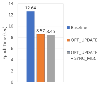
(a)

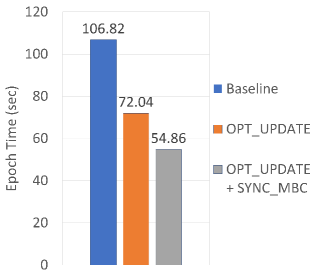
(b)

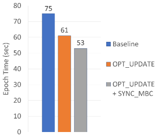
(c)

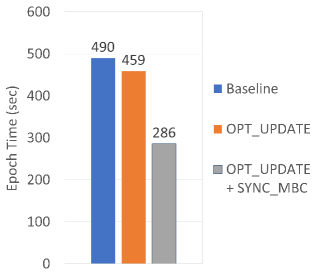
(d)

Figure 2. Comparison of single-socket CPU epoch time of DGL baseline with our optimized GraphSAGE and GAT models using OGBN datasets. We use batch size of $1000$. Baseline is the original DGL execution time. OPT_UPDATE is the execution time with our UPDATE optimizations. OPT_UPDATE + SYNC_MBC is the execution time with parallel synchronized minibatch sampler. OPT_UPDATE for GAT incorporates optimized Broadcast operation. Labels at the top of the bars are epoch time.

4.4. Multi-Socket Performance for DistGNN-MB

In this section, we discuss performance results, including execution time and scaling of our distributed algorithms, and discuss key factors impacting their efficiency. We maintain the following HEC parameter settings throughout our experiments: HEC size ($cs$) is $1$M entries, Cache-line communication threshold ($nc$) is $2000$, Cache-line life-span ($ls$) is $2$, and Communication Delay ($d$) is $1$ iteration.

During model training, epoch time consists of the following components: minibatch creation time (MBC), forward pass time (FWD), backpropagation time (BWD), and MPI All-Reduce time (ARed) to aggregate model parameter gradients. FWD components, in addition to forward pass compute, also encompass remote aggregation time (pre-processing, communication and post-processing). Figures 3 and  4 show the epoch time (including its components) and speedup of GraphSAGE and GAT models on OGBN datasets.

GraphSAGE on OGBN-Papers100M, epoch time consistently diminishes as we scale the number of ranks from $4$ – $64$, with best epoch time of $2$ sec at $64$ ranks. At $64$ ranks, GraphSAGE achieves best relative speedup (w.r.t. $4$ ranks) of $10\times$. Among the components of epoch time, MBC and BWD scale perfectly linearly, while FWD and ARed run at 40% and 69% scaling efficiency from $4$ - - $64$ ranks, respectively. While HEC is able to completely hide the communication cost with a delay of $1$, pre- and post-processing time for communication starts dominating FWD with increase in scale. For example, with increasing number of ranks, more iterations over constant time Map (Algorithm 2) function leads to higher communication processing time. On OGBN-Products, GraphSAGE achieves $7.5\times$ speedup (w.r.t. $2$ ranks) on $16$ ranks.

For GAT, we see similar performance behaviour as GraphSAGE. On OGBN-Papers100M, it showcases the best epoch time of $4.9$ sec at $64$ ranks. At $64$ ranks, GAT achieves best relative speedup (w.r.t $4$ ranks) of $17.2\times$.

BWD dominates GAT epoch time, followed by compute part of FWD. Using HE leads to lowering of required compute. Consequently, we see greater than 100% parallel efficiency as we scale from $4$ – $64$ ranks. MBC and BWD scale perfectly linearly. FWD (due to pre- and post-processing for communication) and ARed run at 74% and 85% scaling efficiency, respectively, from $4$ – $64$ ranks. Due to efficient BWD scaling, FWD time dominates at $64$ ranks. On OGBN-Products, GAT shows $21.9\times$ speedup (w.r.t. $2$ ranks) on $32$ ranks.

On HEC utilization, we empirically observe that HEC hit-rate at $64$ ranks under chosen parameter settings ($cs=1M/layer$, $ls=2$, $nc=2000$ and $d=1$) is 71%, 47%, and 37% at layers L₀, L₁, and L₂, respectively.

Load Imbalance. Multiple factors and their combinations lead to load imbalance in minibatch execution time. Uneven distribution of training examples (even after balancing attempts) among the partitions due to graph partition directly contributes to imbalance during training. For example, at $4$ ranks, lowest and highest minibatch counts across ranks are $264$ and $315$, respectively. Better distribution of training vertices during partitioning can alleviate the load imbalance problem. Other, complex factors include number of halo vertices (or solid vertices) and cache hit-rate. From $4$–$64$ ranks, we observe maximum load imbalance of 12% and 8.7% for GraphSAGE and GAT, respectively.

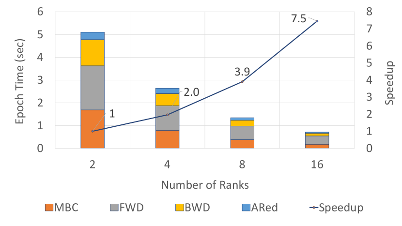
OGBN-Products

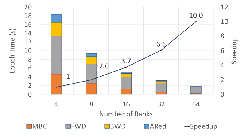
OGBN-Papers100M

Figure 3. Epoch time (in sec) and relative speedup for GraphSAGE from $2$ to $64$ ranks on OGBN datasets

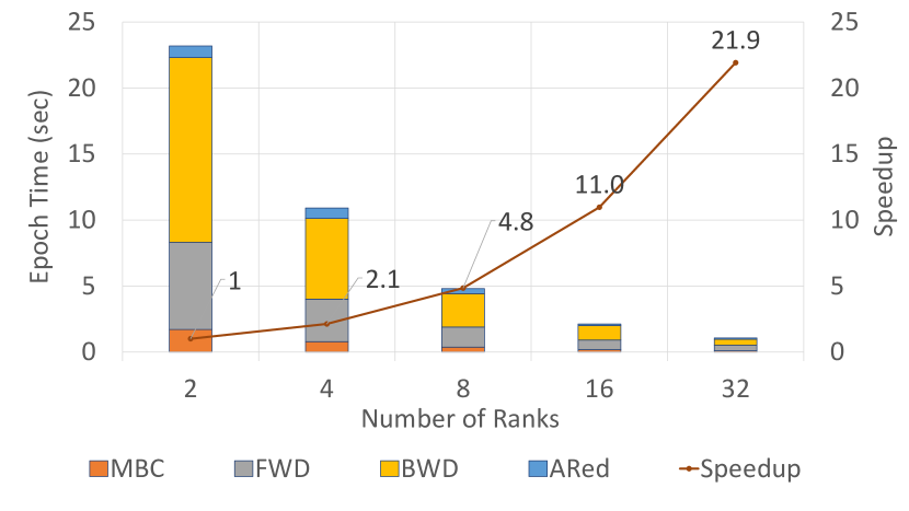
OGBN-Products

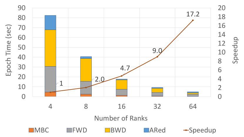
OGBN-Papers100M

Figure 4. Epoch time (in sec) and relative speedup for GAT from $2$ to $64$ ranks on OGBN datasets

4.5. Convergence

We establish single-socket CPU test accuracy (by training for $20$ and $50$ epochs for OGBN-Products and OGBN-Papers100M) as target accuracy to assess the distributed training convergence (Table 3).

Table 3. Target test accuracy of GraphSAGE and GAT on OGBN datasets.

	Test Accuracy (%)
Model/Dataset	OGBN-Products	OGBN-Papers100M
GraphSAGE	$78.2$	$65$
GAT	$78.5$	$65$

We train the model till it achieves test accuracy within $1\%$ of the target accuracy (i.e., $target$ $accuracy-model$ $accuracy<1\%$). In single-socket CPU runs, GraphSAGE converges at $7^{th}$ and $9^{th}$ epoch on OGBN-Products and OGBN-Papers100M, respectively; GAT converges at $6^{th}$ epoch for both the datasets. In our distributed experiments, we observe that GraphSAGE converges at the $30^{th}$ on OGBN-Products for $16$ ranks, and at the $15^{th}$ epoch on OGBN-Papers100M for $64$ ranks. Similarly, we observe that GAT converges at the $20^{th}$ on OGBN-Products for $32$ ranks, and at the $26^{th}$ epoch on OGBN-Papers100M for $64$ ranks.

4.6. Comparison with DistDGL

In this section, we compare the performance of DistGNN-MB with state-of-the-art DistDGL (Zheng et al., 2020) for GraphSAGE. We ran GraphSAGE on DistDGL in our experimental setup following DistDGL instructions. For DistDGL, we used the exact same parameter settings as used in DistGNN-MB (described in section 4.2). Additionally, we used $2$ samplers, $1$ trainer, and $1$ server after limited tuning. Figure 5 shows per epoch time comparison on OGBN datasets between DistGNN-MB and DistDGL. DistGNN-MB consistently performs better than DistDGL on both the datasets from $8$– $64$ ranks. At $64$ ranks, DistGNN-MB achieves speedup of $5.2\times$ per epoch over DistDGL.

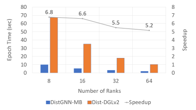
Figure 5. Performance comparison of DistGNN-MB with DistDGL from $8$ to $64$ ranks using GraphSAGE mode on OGBN-Papers100M. We used $2$ sampler, $1$ trainer, and $1$ server for DistDGL experiments.

5. Related Work

Distributed GNN training is an important topic, ongoing research on batch creation, improving compute efficiency and mitigating communication overhead, improving model accuracy etc. In this section, we discuss specific efforts on training via minibatch sampling, including work on using historical embeddings, and compute-communication overlap in this setting (i.e., minibatch training).

DistDGL (Zheng et al., 2020) is a distributed training architecture built on top of the Deep Graph Library (DGL); it employs a set of processes to perform distributed neighbor sampling and feature communication, a distributed key-value-store (KVStore) to hold vertex and edge features/embeddings, and a set of compute resources (processes/threads) to perform model training. It uses METIS (Karypis and Kumar, 1997) to partition the input graph using minimum edge-cut algorithm, but also to balance training example vertices as well as edges across machines.

Although Sancus (Peng et al., 2022) focuses on full-graph training on GPUs, we discuss their historical embedding technique that is "staleness-aware" and designed to reduce communication while maintaining accuracy. Sancus distributes both the adjacency matrix and node features tensor across GPUs; a "root" GPU performs a staleness-check and triggers node-feature-broadcast across all GPUs if embeddings become "too stale", but within staleness bounds all GPUs use embeddings they compute locally, to train the model. They discuss a theoretical proof that bounded staleness does not result in accuracy loss.

In (Ramezani et al., 2022), the authors propose a mechanism to ignore cut-edges that resulted in partitions, and applying on LocalSGD algorithm to compute model gradients during minibatch training in a distributed setting. At the end of every training iteration, each machine communicates it’s local gradients to a global server that contains the full graph; the server corrects local gradients by constructing a minibatch with full neighborhood, computing a stochastic gradient, and updating model parameters which it broadcasts back to all machines.

In (Zeng et al., 2021) and (Zeng et al., 2020), the authors propose graph sampling from the original un-partitioned graph, constructing a GNN on the sampled graph and training the model using each graph sample as a minibatch. They describe algorithms to eliminate the bias introduced by graph sampling and parallelization strategies to improve performance of this operation. Because they construct a full GNN on each sample, they do not need to communicate features during training. They also parallelize forward and backpropagation passes on each minibatch during training.

The Dorylus (Thorpe et al., 2021) distributed system for training GNNs separates computation into "graph parallel" and "tensor parallel" tasks, executing the former on regular CPU instances and the latter on Lambda threads (low-cost, serverless threads) in an AWS environment. To ensure overlap between the two computation types, this work introduces bounded pipeline asynchronous computation to hide the latency incurred due to Lambda threads.

$P^{3}$ (Gandhi and Iyer, 2021) uses a combination of model, data and pipelined parallelism to efficiently execute distributed GNN training on GPUs. It focuses on eliminating feature communication for the largest layer of the computational graph via model parallelism (i.e., each GPU owns part of the vertex features) and employing data parallelism at all other layers. To further mitigate GPU stalls due to lack of compute-communication overlap, $P^{3}$ implements pipelined parallelism.

ByteGNN (Zheng et al., 2022) is a distributed GNN training framework targeting efficient training performance on CPUs, with a primary focus on effectively scheduling minibatch creation tasks (including sampling, sub-graph creation and feature fetch) to overlap with model computation. To support the primary focus, this work also describes a graph partitioning algorithm that attempts to maintain data locality based on minibatch sampling data access patterns.

6. Conclusions and Future Work

Large-scale graph structure learning by training GNN models is a very important technique that is growing in applicability and popularity, as many real-world data can be represented as graphs. To match the increasing scale of these graphs – both in terms of size and quantity – practitioners must develop techniques to improve GNN model training quality and speed. In this paper, we demonstrate the ability of a cluster of CPUs based on the 3rd generation Intel Xeon Scalable Processors to train two popular GNN models, GraphSAGE and GAT, to convergence at high-speed. To achieve these results, we developed a novel compute-communication overlap algorithm to reduce overhead at scale, a novel software-managed Historical Embedding Cache to reduce communications without accuracy impact, and performance optimizations to the AGG primitive in DGL and the UPDATE primitive via a separate Pytorch C++ extension. As part of future work, we will expand benchmark coverage to demonstrate DistGNN-MB’s wider applicability. We will also demonstrate DistGNN-MB performance on the upcoming 4th generation Intel Xeon Scalable Processors with Advanced Matrix Instruction (AMX) and BFloat16 data-type support.

References

- (1)
- Chen et al. (2017) Jianfei Chen, Jun Zhu, and Le Song. 2017. Stochastic training of graph convolutional networks with variance reduction. arXiv preprint arXiv:1710.10568 (2017).
- Fey et al. (2021) Matthias Fey, Jan E Lenssen, Frank Weichert, and Jure Leskovec. 2021. Gnnautoscale: Scalable and expressive graph neural networks via historical embeddings. In International Conference on Machine Learning. PMLR, 3294–3304.
- Gandhi and Iyer (2021) Swapnil Gandhi and Anand Padmanabha Iyer. 2021. P3: Distributed deep graph learning at scale. In 15th USENIX Symposium on Operating Systems Design and Implementation (OSDI 21). 551–568.
- Georganas et al. (2021) Evangelos Georganas, Dhiraj Kalamkar, Sasikanth Avancha, Menachem Adelman, Cristina Anderson, Alexander Breuer, Jeremy Bruestle, Narendra Chaudhary, Abhisek Kundu, Denise Kutnick, Frank Laub, Vasimuddin Md, Sanchit Misra, Ramanarayan Mohanty, Hans Pabst, Barukh Ziv, and Alexander Heinecke. 2021. Tensor Processing Primitives: A Programming Abstraction for Efficiency and Portability in Deep Learning Workloads. In Proceedings of the International Conference for High Performance Computing, Networking, Storage and Analysis (St. Louis, Missouri) (SC ’21). Association for Computing Machinery, New York, NY, USA, Article 14, 14 pages. https://doi.org/10.1145/3458817.3476206
- Hamilton et al. (2017) William L Hamilton, Rex Ying, and Jure Leskovec. 2017. Inductive representation learning on large graphs. In Proceedings of the 31st International Conference on Neural Information Processing Systems. 1025–1035.
- Hu et al. (2020) Weihua Hu, Matthias Fey, Marinka Zitnik, Yuxiao Dong, Hongyu Ren, Bowen Liu, Michele Catasta, and Jure Leskovec. 2020. Open Graph Benchmark: Datasets for Machine Learning on Graphs. arXiv preprint arXiv:2005.00687 (2020).
- Karypis and Kumar (1997) George Karypis and Vipin Kumar. 1997. METIS: A software package for partitioning unstructured graphs, partitioning meshes, and computing fill-reducing orderings of sparse matrices. (1997).
- Karypis et al. (1997) George Karypis, Kirk Schloegel, and Vipin Kumar. 1997. Parmetis: Parallel graph partitioning and sparse matrix ordering library. (1997).
- Liu et al. (2021) Yang Liu, Xiang Ao, Zidi Qin, Jianfeng Chi, Jinghua Feng, Hao Yang, and Qing He. 2021. Pick and Choose: A GNN-Based Imbalanced Learning Approach for Fraud Detection. In Proceedings of the Web Conference 2021 (Ljubljana, Slovenia) (WWW ’21). Association for Computing Machinery, New York, NY, USA, 3168–3177. https://doi.org/10.1145/3442381.3449989
- Peng et al. (2022) Jingshu Peng, Zhao Chen, Yingxia Shao, Yanyan Shen, Lei Chen, and Jiannong Cao. 2022. Sancus: Staleness-Aware Communication-Avoiding Full-Graph Decentralized Training in Large-Scale Graph Neural Networks. Proc. VLDB Endow. 15, 9 (may 2022), 1937–1950. https://doi.org/10.14778/3538598.3538614
- Ramezani et al. (2022) Morteza Ramezani, Weilin Cong, Mehrdad Mahdavi, Mahmut Kandemir, and Anand Sivasubramaniam. 2022. Learn Locally, Correct Globally: A Distributed Algorithm for Training Graph Neural Networks. In International Conference on Learning Representations. https://openreview.net/forum?id=FndDxSz3LxQ
- Thorpe et al. (2021) John Thorpe, Yifan Qiao, Jonathan Eyolfson, Shen Teng, Guanzhou Hu, Zhihao Jia, Jinliang Wei, Keval Vora, Ravi Netravali, Miryung Kim, and Guoqing Harry Xu. 2021. Dorylus: Affordable, Scalable, and Accurate GNN Training with Distributed CPU Servers and Serverless Threads. In 15th USENIX Symposium on Operating Systems Design and Implementation (OSDI 21). USENIX Association, 495–514. https://www.usenix.org/conference/osdi21/presentation/thorpe
- Veličković et al. (2018) Petar Veličković, Guillem Cucurull, Arantxa Casanova, Adriana Romero, Pietro Liò, and Yoshua Bengio. 2018. Graph Attention Networks. International Conference on Learning Representations (2018). https://openreview.net/forum?id=rJXMpikCZ
- Xie et al. (2014) Cong Xie, Ling Yan, Wu-Jun Li, and Zhihua Zhang. 2014. Distributed Power-law Graph Computing: Theoretical and Empirical Analysis.. In Nips, Vol. 27. 1673–1681.
- Ying et al. (2018) Rex Ying, Ruining He, Kaifeng Chen, Pong Eksombatchai, William L Hamilton, and Jure Leskovec. 2018. Graph convolutional neural networks for web-scale recommender systems. In Proceedings of the 24th ACM SIGKDD International Conference on Knowledge Discovery & Data Mining. 974–983.
- Zeng et al. (2020) Hanqing Zeng, Hongkuan Zhou, Ajitesh Srivastava, Rajgopal Kannan, and Viktor Prasanna. 2020. GraphSAINT: Graph Sampling Based Inductive Learning Method. In International Conference on Learning Representations. https://openreview.net/forum?id=BJe8pkHFwS
- Zeng et al. (2021) Hanqing Zeng, Hongkuan Zhou, Ajitesh Srivastava, Rajgopal Kannan, and Viktor Prasanna. 2021. Accurate, efficient and scalable training of Graph Neural Networks. J. Parallel and Distrib. Comput. 147 (2021), 166–183. https://doi.org/10.1016/j.jpdc.2020.08.011
- Zheng et al. (2022) Chenguang Zheng, Hongzhi Chen, Yuxuan Cheng, Zhezheng Song, Yifan Wu, Changji Li, James Cheng, Hao Yang, and Shuai Zhang. 2022. ByteGNN: Efficient Graph Neural Network Training at Large Scale. Proc. VLDB Endow. 15, 6 (feb 2022), 1228–1242. https://doi.org/10.14778/3514061.3514069
- Zheng et al. (2020) Da Zheng, Chao Ma, Minjie Wang, Jinjing Zhou, Qidong Su, Xiang Song, Quan Gan, Zheng Zhang, and George Karypis. 2020. Distdgl: distributed graph neural network training for billion-scale graphs. In 2020 IEEE/ACM 10th Workshop on Irregular Applications: Architectures and Algorithms (IA3). IEEE, 36–44.
- Zitnik et al. (2018) Marinka Zitnik, Monica Agrawal, and Jure Leskovec. 2018. Modeling polypharmacy side effects with graph convolutional networks. Bioinformatics 34, 13 (2018), i457–i466.