Bayesian Integrity Monitoring for Cellular Positioning — A Simplified Case Study

Abstract

Bayesian receiver autonomous integrity monitoring (RAIM) algorithms are developed for the snapshot cellular positioning problem in a simplified one-dimensional (1D) linear Gaussian setting. Position estimation, multi-fault detection and exclusion, and protection level (PL) computation are enabled by the efficient and exact computation of the position posterior probabilities via message passing along a factor graph. Computer simulations demonstrate the significant performance improvement of the proposed Bayesian RAIM algorithms over a baseline advanced RAIM algorithm, as it obtains tighter PLs that meet the target integrity risk (TIR) requirements.

I Introduction

The estimation of position and its associated confidence level is central to numerous engineering applications. One can intuitively understand the utility of receiving both a position estimate and a confidence estimate by the blue circle with changing radius around the ego position in smartphone navigation [1]. Integrity assurance mechanisms and receiver autonomous integrity monitoring (RAIM) algorithms have long been introduced into global navigation satellite systems [2] to ensure a high degree of confidence in the information provided by the systems to the end user. Safety-critical applications in aviation [3], rail [4], and automotive [5] benefit greatly from strong integrity guarantees in positioning systems. The rigorous quantification of integrity is typically done through the formulation of an upper bound of instantaneous position error, termed protection level (PL), to meet the required confidence level (i.e. the probability that the actual error is below PL), often given in the form of one minus the so-called target integrity risk (TIR). It is expected that the computed PLs are tight enough so that their utility in other applications can be maximized [6].

As new safety-critical applications emerge in urban and indoor scenarios, where GNSSs suffers from poor coverage, cellular positioning [7] promises to provide a reliable complementary solution, for which integrity support becomes crucial [8, 9]. In [8], the importance of integrity for cellular localization is argued. Specific errors such as multipath biases and blockages are studied in [9] and mitigated using RAIM. Integrity support for GNSS assistance has been incorporated into the latest 3GPP Release-17 standard [10], and radio standalone positioning with integrity guarantee is expected from Release-18 onward [11]. This emphasizes the importance of RAIM methods for cellular positioning, providing integrity guarantees and tight PLs at the same time.

RAIM methods can be grouped into traditional RAIM algorithms and Bayesian RAIM methods. Traditional RAIM algorithms detect and exclude faulty measurements by performing rounds of consistency checks on the statistics (e.g. range residuals and position estimates) associated with the fault patterns (i.e. the alternative hypotheses in the language of statistical hypothesis testing) that would otherwise lead to large errors [12]. This frequentist approach relies on redundant measurements and does not directly lead to instantaneous position error probability distributions. To avoid underestimating tail risk, the formulation of solvable PL equations has to conservatively overbound the error distribution. Consequently, the computed PLs tends to be loose. In contrast, Bayesian RAIM methods [13, 14, 15, 16] aim to find the posterior probability distribution of position error directly based on the information contained in the measurement models (prior) and actual measurements (evidence). It can be expected that the computed PLs are tight, since, in theory, all the position information contained in the measurements can be preserved in the posterior. The downside of Bayesian RAIM is its potentially high complexity associated with posterior computation, particularly when the number of unknown parameters is large and the problem model admits no closed-form expressions (which, unfortunately, is the general situation). Therefore, a major challenge of Bayesian methods is to find computationally efficient implementations. To date, research work on Bayesian RAIM methods is still very limited, and most of them have adopted Monte Carlo algorithms, such as particle filters [15, 16] and Gibbs sampler [14], for posterior distribution computation.

In this paper, we consider the RAIM problem for snapshot cellular positioning, providing three distinct contributions: (i) we propose a novel factor graph-based Bayesian RAIM method to compute position and PL, including multi-fault detection and exclusion; (ii) we evaluate the method in a simplified one-dimensional (1D) linear Gaussian scenario and compare its performance with a baseline advanced RAIM algorithm [3] using Monte-Carlo simulation; (iii) we demonstrate that, while fulfilling the TIR requirement, the resultant PLs are much tighter than the baseline algorithm due to the exact computation of the posterior probability density by the new method, thus greatly improving the availability of the system.

II Problem Formulation

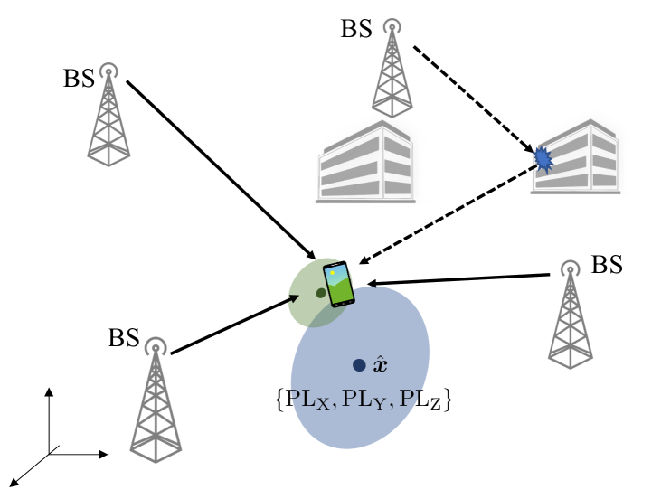
Figure 1: Illustration of the cellular positioning with integrity monitoring problem. In the displayed scenario, one BS is in NLoS condition due to blockage and causes a large bias to the pseudo-range measurement. When a RAIM algorithm failed to exclude this faulty measurement, the computed position estimate $\hat{\bm{x}}$ and PLs $\{\mathrm{PL}_{\mathrm{X}},\mathrm{PL}_{\mathrm{Y}},\mathrm{PL}_{\mathrm{Z}}\}$ are represented by the blue ellipsoid are obtained; when it excludes the faulty measurement successfully, better results represented by the green ellipsoid are obtained.

In this section, we describe the snapshot three-dimensional (3D) positioning and integrity monitoring problem and its simplified 1D version.

II-A The Snapshot Integrity Monitoring Problem

We consider a scenario with $M$ time-synchronized BSs with known locations $\bm{x}_{i}\in\mathbb{R}^{3}$, $i\in\mathcal{I}\triangleq\{1,\ldots,M\}$, and a single mobile user equipment (UE) with unknown position $\bm{x}=[x_{\mathrm{X}},x_{\mathrm{Y}},x_{\mathrm{Z}}]^{\mathrm{T}}\in\mathbb{R}^{3}$ and unknown clock bias $C\in\mathbb{R}$ (expressed in meters). Considering downlink/user-centric positioning, at each positioning epoch the BSs send coordinated positioning reference signals, from which the UE estimates $M$ time-of-arrivals from the line-of-sight (LoS) paths, which are converted to pseudo-ranges as follows:

$$y_{i}=\|\bm{x}_{i}-\bm{x}\|+C+b_{i}+n_{i},$$ (1)

for $i\in\mathcal{I}$, where $n_{i}$ is the independent measurement noise and $b_{i}$ is the range bias that accounts for any possible faults, such as synchronization errors or NLoS biases. We further consider that an initial estimate of the UE position is available, so that (1) can be linearized [17, 18, 19] to yield (after removing unnecessary terms)

$$y_{i}=\bm{a}_{i}^{\mathrm{T}}\begin{bmatrix}\bm{x}\\ C\end{bmatrix}+b_{i}+n_{i},$$ (2)

where $\bm{a}_{i}\in\mathbb{R}^{4\times 1}$ is a known vector. The objective of integrity monitoring is to calculate a position estimate $\hat{\bm{x}}$ and a PL for each dimension $n$ in $\{\mathrm{X},\mathrm{Y},\mathrm{Z}\}$ such that

$$\mathrm{Pr}(|x_{n}-\hat{x}_{n}|>\mathrm{PL}_{n})\leq\mathrm{TIR}_{n},$$ (3)

where $\mathrm{Pr}(|x_{n}-\hat{x}_{n}|>\mathrm{PL}_{n})$ is the actual integrity risk (IR) and $\mathrm{TIR}_{n}$ the TIR for dimension $n$. A schematic drawing of the problem is shown in Fig. 1.

II-B Simplified Problem

Inspired by the observation from (3), that the PL is computed per dimension, we propose a simplified observation model, with the purpose of understanding the possible gains of Bayesian integrity monitoring over conventional frequentist approaches. In its most simple and nontrivial version, that is, a 1D positioning problem without clock bias and with Gaussian error, the 1D model analogy to (2) is

$$y_{i}=x+b_{i}+n_{i},$$ (4)

where $x$, $b_{i}$, and $n_{i}$, for $i\in\mathcal{I}$, are independent random variables. The measurement noise is modeled as $n_{i}\sim\mathcal{N}(n_{i},0,\sigma_{n,i}^{2})$, where the notation $\mathcal{N}(t;m,\sigma^{2})$ represents the Gaussian distribution for the random variable $t$ with mean $m$ and variance $\sigma^{2}$. A latent variable $\lambda_{i}\in\{0,1\}$ is adopted as an indicator of whether the measurement $y_{i}$ is faulty or not, which follows a Bernoulli probability mass function (PMF) given by $p_{\Lambda_{i}}(\lambda_{i})=\theta_{i}^{\lambda_{i}}(1-\theta_{i})^{(1-\lambda_{i})}$, where $\theta_{i}$ is a known prior probability and $0<\theta_{i}\ll 1$ is assumed. When $\lambda_{i}=0$, $y_{i}$ is free from fault and hence $b_{i}=0$. When $\lambda_{i}=1$, $b_{i}$ is modeled as a Gaussian random variable $\mathcal{N}(b_{i};m_{b,i},\sigma_{b,i}^{2})$, whose variance $\sigma_{b,i}^{2}$ is considered considerably greater than $\sigma_{n,i}^{2}$. Consequently, the prior probability density function (PDF) of $b_{i}$ is given by

$$p_{B_{i}}(b_{i}) =p_{B_{i}\mid\Lambda_{i}}(b_{i}\mid 0)\,p_{\Lambda_{i}}(0)+p_{B_{i}\mid\Lambda_{i}}(b_{i}\mid 1)\,p_{\Lambda_{i}}(1)$$

$$=(1-\theta_{i})\delta(b_{i})+\theta_{i}\,\mathcal{N}(b_{i};m_{b,i},\sigma_{b,i}^{2}),$$ (5)

where $\delta(\cdot)$ denotes the Dirac delta distribution. The objective is then to find a position estimate $\hat{x}$ and a PL such that

$$\mathrm{Pr}(|x-\hat{x}|>\mathrm{PL})\leq\mathrm{TIR}.$$ (6)

III Baseline RAIM Solution

For performance benchmarking purposes, we modify the hypothesis testing-based advanced RAIM algorithm [3] to the 1D problem described above. The original algorithm was developed in a multi-fault and multi-constellation GNSS setting. The algorithm has four components: (i) computation of the so-called all-in-view solution based on all $M$ measurements; (ii) identification of the fault modes that will be monitored, that is, which combination of BSs will be considered; (iii) detection of the faults and computation of PL if no faults were detected; (iv) exclusion of possibly faulty measurements if faults were detected and computation of PL.

III-A All-in-View Solution

We rewrite the measurement model (4) in vector form:

$$\bm{y}=\bm{1}_{M}x+\bm{z},$$ (7)

where $\bm{y}=[y_{1},\ldots,y_{M}]^{\mathrm{T}}$, $\bm{1}_{M}$ is a $M\times 1$ all-one vector and $\bm{z}=[z_{1},\ldots,z_{M}]^{\mathrm{T}}$ with elements $z_{i}=b_{i}+n_{i}$, $i=1,\ldots,M$. When all measurements are free of fault, $\bm{z}\sim\mathcal{N}(\bm{0},\bm{\Sigma})$, where $\bm{\Sigma}$ is the diagonal covariance matrix with diagonals $\bm{\Sigma}_{i,i}=\sigma_{n,i}^{2}$, $i=1,\ldots,M$, and the weighted least squares (WLS) estimate for $x$, which in this case also is the maximum likelihood (ML) estimate, is given by

$$\hat{x}^{(0)}=\left(\bm{1}_{M}^{\mathrm{T}}\bm{\Sigma}^{-1}\bm{1}_{M}\right)^{-1}\bm{1}_{M}^{\mathrm{T}}\bm{\Sigma}^{-1}\bm{y}=W_{0}\bm{c}_{0}^{\mathrm{T}}\bm{y},$$ (8)

where $W_{0}\triangleq\left(\bm{1}_{M}^{\mathrm{T}}\bm{\Sigma}^{-1}\bm{1}_{M}\right)^{-1}={\big{(}\sum_{i=1}^{M}{\sigma_{n,i}^{-2}}\big{)}}^{-1}$, and $\bm{c}_{0}^{\mathrm{T}}\triangleq\bm{1}_{M}^{\mathrm{T}}\bm{\Sigma}^{-1}=[{\sigma_{n,1}^{-2}},\ldots,{\sigma_{n,M}^{-2}}]$.

III-B Fault Modes Identification

First, the baseline RAIM algorithm determines the set of fault modes to be monitored, based on prior knowledge of the probability that each measurement is faulty. A fault mode is a specific subset of measurements that are simultaneously faulty, while the rest of the measurements are fault-free. The baseline algorithm lists all fault modes that contain up to $M-2$ measurements and computes the corresponding probabilities of occurrence. Therefore, the total number of fault modes is given by $N_{\mathrm{FM}}=\sum_{j=1}^{M-2}\binom{M}{j}$. For convenience, the fault-free case (i.e., the null hypothesis) is denoted as the fault mode $0$. We denote by $\mathcal{I}_{k}$ the set of faulty measurement indices contained in the fault mode $k\in\{0,1,\ldots,N_{\mathrm{FM}}\}$. In particular, $\mathcal{I}_{0}=\emptyset$. The probability that this fault mode occurs is thus given by

$$p_{\mathrm{FM},k}=\prod_{i\in\mathcal{I}_{k}}\theta_{i}\prod_{i\in\mathcal{I}\setminus\mathcal{I}_{k}}(1-\theta_{i}).$$ (9)

Fault modes are sorted in decreasing order of their probability of occurrence. Namely, $p_{\mathrm{FM},k}\geq p_{\mathrm{FM},k+1}$, for $k<N_{\mathrm{FM}}$. Note that since $0<\theta_{i}\ll 1$ is commonly assumed, $p_{\mathrm{FM},0}>p_{\mathrm{FM},1}$ is considered true.

We note that to ensure the best possible performance, all fault modes that can be monitored are listed in this baseline RAIM algorithm. In the original algorithm described in [3], those fault modes that contain a large number of faulty measurements but with a very small probability of occurrence are left out of the monitoring, so that the computational complexity of the algorithm can be reduced. We refer the interested readers to [3] for more details.

III-C Fault Detection

For fault mode $k$, we define $W_{k}\triangleq{\big{(}\sum_{i\in\mathcal{I}\setminus\mathcal{I}_{k}}{\sigma_{n,i}^{-2}}\big{)}}^{-1}$ and let $\bm{c}_{k}^{\mathrm{T}}$ to be the vector given by replacing elements of $\bm{c}_{0}^{\mathrm{T}}$ with indices in $\mathcal{I}_{k}$ by $0$. It can be easily verified that

$$\hat{x}^{(k)}=W_{k}\bm{c}_{k}^{\mathrm{T}}\bm{y}$$ (10)

is the WLS estimate of $x$ using the remaining measures after excluding those contained in fault mode $k$ from $\bm{y}$.

The baseline RAIM algorithm determines whether the measurements contain faults by performing a list of solution separation (SS) tests for each fault mode. When all measurements are fault-free, it can be shown that the test statistic $\Delta\hat{x}^{(k)}\triangleq\hat{x}^{(0)}-\hat{x}^{(k)}$ is a Gaussian random variable with zero mean and variance given by

$$\sigma_{ss}^{(k)2}\triangleq\left(W_{k}\bm{c}_{k}^{\mathrm{T}}-W_{0}\bm{c}_{0}^{\mathrm{T}}\right)\bm{\Sigma}\left(W_{k}\bm{c}_{k}^{\mathrm{T}}-W_{0}\bm{c}_{0}^{\mathrm{T}}\right)^{\mathrm{T}}.$$ (11)

To be able to identify the test thresholds, a false alarm probability $P_{\mathrm{FA}}$ is also required as input to the algorithm. The false alarm budget is evenly allocated to the $N_{\mathrm{FM}}$ fault modes that contain fault(s), leading to the following SS test threshold for fault mode $k$, $k=1,\ldots,N_{\mathrm{FM}}$,

$$T_{k}=\sigma_{ss}^{(k)}\,Q^{-1}\left(\frac{P_{\mathrm{FA}}}{2N_{\mathrm{FM}}}\right),$$ (12)

where $Q^{-1}(\cdot)$ is the inverse of the $Q$ function, $Q(u)=\frac{1}{\sqrt{2\pi}}\int_{u}^{+\infty}e^{-\frac{t^{2}}{2}}\mathrm{d}t$. To be specific, $|\Delta\hat{x}^{(k)}|$ will be compared with $T_{k}$, and if $|\Delta\hat{x}^{(k)}|\leq T_{k}$, $\forall k=1,\ldots,N_{\mathrm{FM}}$, all measurements are considered fault-free and the baseline RAIM algorithm outputs $\hat{x}^{(0)}$ as the position estimate. The choice of $P_{\mathrm{FA}}$, therefore, affects the continuity and availability performance of the positioning system: the larger the value, the more likely the algorithm is to warn upon a potential fault and will put more computational effort into fault exclusion attempts.

A PL is computed by solving the following equation:

$$2Q\left(\frac{\mathrm{PL}}{\sigma^{(0)}}\right)+\sum_{k=1}^{N_{\mathrm{FM}}}p_{\mathrm{FM},k}\,Q\left(\frac{\mathrm{PL}-T_{k}}{\sigma^{(k)}}\right)=\mathrm{TIR},$$ (13)

where $\sigma^{(k)}\triangleq W_{k}\sqrt{\bm{c}_{k}^{\mathrm{T}}\bm{\Sigma}\bm{c}_{k}}$, and $Q\left(\frac{\mathrm{PL}-T_{k}}{\sigma^{(k)}}\right)$ is an upper bound of the actual IR when fault mode $k$ occurs but the SS test passes, i.e., $\mathrm{Pr}(|x-\hat{x}^{(0)}|>\mathrm{PL},|\hat{x}^{(0)}-\hat{x}^{(k)}|\leq T_{k})$. The formulation process of the above equation can be found in [3, Appendix H], and a solution of (13) is found using the bisection search method detailed in [3, Appendix B].

III-D Fault Exclusion

When any SS tests fail, that is, $|\Delta\hat{x}^{(k)}|>T_{k}$ for some $k$, the baseline RAIM algorithm will try to exclude faulty measurements that cause failure. Starting from $k=1$, the algorithm performs the complete process of fault modes identification and fault detection on the new problem formed after removing the measurements contained in fault mode $k$. The remaining number of measurements in this new problem is $M-|\mathcal{I}_{k}|$. If the SS tests pass successfully, the fault exclusion process is terminated and a PL can be computed in the same way as described above (but using the newly obtained values for $p_{\mathrm{FM},k}$, $T_{k}$, $N_{\mathrm{FM}}$, etc.). Otherwise, the algorithm continues to check the next fault mode ($k+1$). If the SS tests fail for all fault modes, then the fault exclusion attempt is considered failed. In this case, the algorithm terminates without being able to compute a PL and should claim that the position estimate should not be trusted.

IV Proposed Bayesian Methods

From a Bayesian perspective, we treat $x$ and $\lambda_{i}$ in (4) as random variables, whose prior probability distributions, $p_{X}(x)$ and $p_{\Lambda_{i}}(\lambda_{i})$, $\forall i\in\mathcal{I}$, are known. For each epoch of the integrity monitoring problem, we aim to determine the marginal posterior distribution of each random variable, i.e., $p_{X|\bm{Y}}(x|\bm{y})$ and $p_{\Lambda_{i}|\bm{Y}}(\lambda_{i}|\bm{y})$, $i\in\mathcal{I}$, from the prior information, the measurements $\bm{y}$, and the corresponding likelihood function induced by (4). Based on the posterior distributions, different methods can be selected to compute the position estimate $\hat{x}$ and PL to meet the TIR requirement.

IV-A Message Passing Algorithm

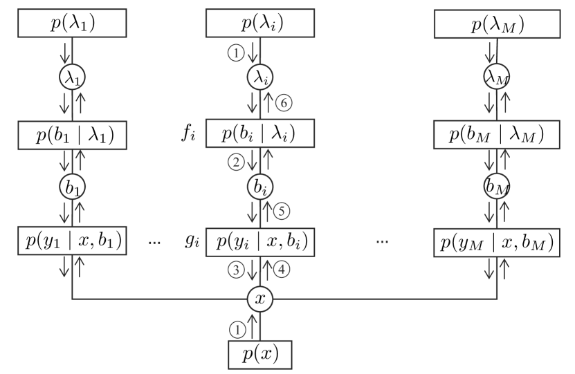
Figure 2: Factor graph of the Bayesian RAIM problem, corresponding to the factorization (14). The order of message computation and passing is given by the numbers in circles (shown only on the $i$th branch, but is the same for all branches), while the arrows indicate the passing direction.

Based on the assumptions made in Section II, the joint posterior probability of $x$, $\bm{b}\triangleq[b_{1},\ldots,b_{M}]^{\mathrm{T}}$ and $\bm{\lambda}\triangleq[\lambda_{1},\ldots,\lambda_{M}]^{\mathrm{T}}$ can be factorized as

$$p(x,\bm{b},\bm{\lambda}\mid\bm{y}) \propto p(\bm{y}\mid x,\bm{b},\bm{\lambda})p(x,\bm{b},\bm{\lambda})$$

$$=p(x)\prod_{i=1}^{M}p(y_{i}\mid x,b_{i})p(b_{i}\mid\lambda_{i})p(\lambda_{i}).$$ (14)

For clarity, the subscripts of the probability distributions are omitted in (14) and all subsequent expressions and the variables to which they belong should be clear from the context.

A cycle-free factor graph representation of (14) is shown in Fig. 2, where each term of (14) is represented by a factor node in a rectangle and connected to the variable nodes that appear in parentheses, represented by circles in the graph. The leaf (factor) nodes are all prior distribution functions. The remaining two categories of factor nodes are the conditional density functions $p(b_{i}|\lambda_{i})$ and $p(y_{i}|x,b_{i})$, which are denoted by $f_{i}$ and $g_{i}$ respectively for simplicity. Since the factor graph is cycle-free, a simple message-passing schedule is applied following the sum-product algorithm [20].

The following notations and operations are involved. $\mathrm{GM}(t,L)$ stands for a Gaussian mixture (GM) distribution for $t$ with $L$ components: $\sum_{l=1}^{L}w_{l}\mathcal{N}(t;m_{l},\sigma_{l}^{2})$ with $\sum_{l=1}^{L}w_{l}=1$. Many messages passed on the factor graph are of this form, and their weights $\{w_{l}\}$, means $\{m_{l}\}$, and standard deviations $\{\sigma_{l}\}$ are what actually needs to be sent. Given $\mathrm{GM}(t,L_{1})=\sum_{l_{1}=1}^{L_{1}}w_{l_{1}}\mathcal{N}(t;m_{l_{1}},\sigma_{l_{1}}^{2})$ and $\mathrm{GM}(t,L_{2})=\sum_{l_{2}=1}^{L_{2}}w_{l_{2}}\mathcal{N}(t;m_{l_{2}},\sigma_{l_{2}}^{2})$, their product is given by

$$\sum_{l_{1}=1}^{L_{1}}\sum_{l_{2}=1}^{L_{2}}w_{l_{1}}w_{l_{2}}s_{l_{1}l_{2}}\,\mathcal{N}(t;m_{l_{1}l_{2}},\sigma_{l_{1}l_{2}}^{2})\propto\mathrm{GM}(t,L_{1}L_{2}),$$ (15)

where $s_{l_{1}l_{2}}$, $m_{l_{1}l_{2}}$ and $\sigma_{l_{1}l_{2}}$ are obtained by solving the following simple equations:

$$\begin{cases}{1}/{\sigma_{l_{1}l_{2}}^{2}}={1}/{\sigma_{l_{1}}^{2}}+{1}/{\sigma_{l_{2}}^{2}},\\ {m_{l_{1}l_{2}}}/{\sigma_{l_{1}l_{2}}^{2}}={m_{l_{1}}}/{\sigma_{l_{1}}^{2}}+{m_{l_{2}}}/{\sigma_{l_{2}}^{2}},\\ s_{l_{1}l_{2}}=\mathcal{N}(m_{l_{1}};m_{l_{2}},\sigma_{l_{1}}^{2}+\sigma_{l_{2}}^{2}).\end{cases}$$ (16)

A limited number of arithmetic operations are needed to solve these equations. Therefore, the computational complexity associated with this product is given by $\mathcal{O}(L_{1}L_{2})$.

The message-passing schedule is described below for the $i$th branch. It proceeds in parallel along all $M$ branches.

1. The prior $p(\lambda_{i})$ is sent from the leaf node to variable nodes $\lambda_{i}$, and then directly to $f_{i}$. Meanwhile, $p(x)$ is sent to the variable node $x$.

2. Factor node $f_{i}$ sends the following message to variable node $b_{i}$:

   $$\mu_{f_{i}\rightarrow b_{i}}(b_{i}) =\sum_{\lambda_{i}}p(b_{i}\mid\lambda_{i})p(\lambda_{i}).$$ (17)

   which is a GM distribution of $b_{i}$, given by $\mu_{f_{i}\rightarrow b_{i}}(b_{i})=(1-\theta_{i})\,\mathcal{N}(b_{i};0,0)+\theta_{i}\,\mathcal{N}(b_{i};m_{b,i},\sigma_{b,i}^{2})$. This message will be passed directly to factor node $g_{i}$.

3. Factor node $g_{i}$ sends the following message to variable node $x$:

   $$\mu_{g_{i}\rightarrow x}(x)=\int p(y_{i}\mid x,b_{i})\,\mu_{f_{i}\rightarrow b_{i}}(b_{i})\,\mathrm{d}b_{i}.$$ (18)

   Since $p(y_{i}|x,b_{i})=\mathcal{N}(b_{i};y_{i}-x,\sigma_{n,i}^{2})$, based on (15) and (16), the integration results in a $\mathrm{GM}(x,2)$ density:

   $$(1-\theta_{i})\,\mathcal{N}(x;y_{i},\sigma_{n,i}^{2})+\theta_{i}\,\mathcal{N}(x;y_{i}-m_{b,i},\sigma_{n,i}^{2}+\sigma_{b,i}^{2}).$$ (19)

4. Variable node $x$ sends the following message back to $g_{i}$:

   $$\mu_{x\rightarrow g_{i}}(x) =p(x)\prod_{j\in\mathcal{M}\setminus i}\mu_{g_{j}\rightarrow x}(x).$$ (20)

   Under the assumption of Gaussian or uniform distribution of $p(x)$, $\mu_{x\rightarrow g_{i}}(x)\propto\mathrm{GM}(x,2^{M-1})$.

5. Factor node $g_{i}$ sends the following message back to $b_{i}$:

   $$\mu_{g_{i}\rightarrow b_{i}}(b_{i}) =\int p(y_{i}\mid x,b_{i})\,\mu_{x\rightarrow g_{i}}(x)\,\mathrm{d}x,$$ (21)

   which is then passed on to factor node $f_{i}$ directly. Since $p(y_{i}|x,b_{i})$ can also be regarded as Gaussian PDF of $x$, i.e., $\mathcal{N}(x;y_{i}-b_{i},\sigma_{n,i}^{2})$, following the same procedure as in step , it is clear that $\mu_{g_{i}\rightarrow b_{i}}(b_{i})\propto\mathrm{GM}(b_{i},2^{M-1})$ and the parameters are easy to compute.

6. Finally, the factor node $f_{i}$ sends a message back to $\lambda_{i}$, which is given by

   $$\mu_{f_{i}\rightarrow\lambda_{i}}(\lambda_{i}) =\int p(b_{i}\mid\lambda_{i})\,\mu_{g_{i}\rightarrow b_{i}}(b_{i})\,\mathrm{d}b_{i}.$$ (22)

   The message is computed separately for $\lambda_{i}=0$ and $\lambda_{i}=1$. In particular, $\mu_{f_{i}\rightarrow\lambda_{i}}(\lambda_{i}=0)=\mu_{g_{i}\rightarrow b_{i}}(b_{i}=0)$, and the computation of $\mu_{f_{i}\rightarrow\lambda_{i}}(\lambda_{i}=1)$ requires $2^{M-1}$ terms of product of two Gaussian in the integrand.

The message-passing process terminates after the above six steps. The marginal posteriors can be calculated by multiplying all the incoming messages at the variable nodes $x$ and $\{\lambda_{i}\}$. In particular,

$$p(x\mid\bm{y})\propto p(x)\prod_{i\in\mathcal{M}}\mu_{g_{i}\rightarrow x}(x),$$ (23)

which leads to a GM distribution with $2^{M}$ terms, and

$$p(\lambda_{i}\mid\bm{y})=\begin{cases}1-\theta_{i}^{\prime}\propto(1\!-\!\theta_{i})\cdot\mu_{f_{i}\rightarrow\lambda_{i}}(\lambda_{i}=0),&\text{if }\lambda_{i}=0,\\ \theta_{i}^{\prime}\hskip 17.07164pt\propto\theta_{i}\cdot\mu_{f_{i}\rightarrow\lambda_{i}}(\lambda_{i}=1),&\text{if }\lambda_{i}=1,\end{cases}$$ (24)

where $\theta_{i}^{\prime}$ can be obtained after normalization.

IV-B Fault Exclusion

In theory, all the information about the user position contained in the measurements and priors has been collected in $p(x|\bm{y})$ given by (23), and a position estimate and a PL can be computed directly based on it. However, the bias term in a faulty measurement will introduce a large uncertainty in the posterior, which will lead to a large PL. To counteract this effect, fault exclusion can be performed based on the marginal posterior PMFs of the indicators given by (24), before computing the marginal posterior PDF of $x$ using the remaining measurements. To be specific, a threshold $\theta_{T}$ is selected, and if $\theta_{i}^{\prime}>\theta_{T}$, the measurement $y_{i}$ is considered faulty, the corresponding branch will be pruned from the factor graph and the message $\mu_{g_{i}\rightarrow x}(x)$ passed to variable node $x$ along it will be discarded. No other additional message computation/passing is required.

Denoting the set of indices of excluded measurements is by $\mathcal{I}_{\mathrm{F}}$, the marginal posterior of $x$ after fault exclusion is computed by

$$p_{\mathrm{FE}}(x\mid\bm{y})\propto p(x)\prod_{i\in\mathcal{I}\setminus\mathcal{I}_{\mathrm{F}}}\mu_{g_{i}\rightarrow x}(x),$$ (25)

which leads to a GM posterior distribution of $2^{M-|\mathcal{I}_{\mathrm{F}}|}$ terms.

IV-C Position Estimation and PL Computation

With or without fault exclusion, the marginal posterior of $x$ can anyway be written in the following form:

$$p_{X}^{\mathrm{pos}}(x)=\sum_{l=1}^{L}w_{x,l}\,\mathcal{N}(x;m_{x,l},\sigma_{x,l}^{2}),$$ (26)

where $\{w_{x,l},l=1,\ldots,L\}$ is sorted in decreasing order and $L$ is either given by $2^{M}$ following (23), or by $2^{M-|\mathcal{I}_{\mathrm{F}}|}$ following (25). For position estimation, the weighted mean (WM) method is adopted, so that $\hat{x}=\sum_{l=1}^{L}w_{x,l}\,m_{x,l}$.

Based on (26), the IR associated with a position estimate $\hat{x}$ and a said PL can be formulated as

$$\mathrm{IR} =\mathrm{Pr}(x<\hat{x}-\mathrm{PL})+\mathrm{Pr}(x>\hat{x}+\mathrm{PL})$$

$$=\sum_{l=1}^{L}w_{x,l}\Big{[}\Phi_{\mathcal{N},l}(\hat{x}-\mathrm{PL})+1-\Phi_{\mathcal{N},l}(\hat{x}+\mathrm{PL})\Big{]},$$ (27)

where $\Phi_{\mathcal{N},l}(\cdot)$ stands for the cumulative density function (CDF) of the $l$th Gaussian term in (26). Using the notation of $Q$ function as in (13), the goal is to find the smallest value for $\mathrm{PL}$ such that the following inequality holds:

$$\sum_{l=1}^{L}w_{x,l}\left[1-Q\Big{(}\frac{\hat{x}\!-\!\mathrm{PL}\!-\!m_{x,l}}{\sigma_{x,l}}\Big{)}+Q\Big{(}\frac{\hat{x}\!+\!\mathrm{PL}\!-\!m_{x,l}}{\sigma_{x,l}}\Big{)}\right]$$

$$\leq\mathrm{TIR}.$$ (28)

For this, a bisection search is again employed by the Bayesian RAIM algorithms.

Depending on whether to perform fault exclusion or not, two variations of the Bayesian RAIM algorithm have resulted under the same framework (labeled using FE or NFE in the numerical study). Their performance will be compared with the baseline RAIM algorithm in the following section. We also remark that other position estimation methods, e.g., maximum a posterior (MAP) estimation, can also be adopted, which can be expected to have an impact on the computed PL according to (28). The comparison of different position estimation methods will be left for future work.

IV-D Computational Complexity Comparison

For all other steps except PL computation, the Bayesian RAIM algorithm has a fixed complexity scaling of $\mathcal{O}(3M\times 2^{M-1})$, mainly due to the computation of (23) via message passing. The baseline RAIM have a variable complexity (as the number of SS test varies), between $\mathcal{O}\left(N_{\mathrm{FM}}\right)$ (when all SS tests pass in the fault detection step) and approximately $\mathcal{O}\left(N_{\mathrm{FM}}^{2}\right)$ (when every fault mode is examined in the fault exclusion step), where $N_{\mathrm{FM}}=\sum_{j=1}^{M-2}\binom{M}{j}=2^{M}-M-2$.

Both methods require a bisection search to compute the PL, which is an iterative algorithm. For a given number of iterations, say $N_{\mathrm{it}}>0$, the complexity of the PL computation in Bayesian RAIM is $\mathcal{O}(N_{\mathrm{it}}2L)$, where $L=2^{M}$ without fault exclusion and $L=2^{M-|\mathcal{I}_{\mathrm{F}}|}$ with fault exclusion. For baseline RAIM, this complexity is $\mathcal{O}(N_{\mathrm{it}}N_{\mathrm{FM}})$.

Remark 1.

In cellular positioning, there are usually few connected BSs ($M\leq 10$). Therefore, the computational complexities of the baseline and proposed Bayesian RAIM algorithms can be said in a similar order for the 1D positioning problem. We note that in GNSS, the number of satellites visible to the UE can be many more, which could entail high computational complexities of the Bayesian algorithms.

V Numerical Study

V-A Scenario

For numerical study, scenarios with $M=5$ or $8$ BSs and one UE are considered. Without loss of generality, the actual position of the UE is always at $x=0$. All BSs have the same measurement noise level $\sigma_{n,i}$ (thus denoted simply using $\sigma_{n}$ in the following discussion), which increases from $1$ to $9$ meters in steps of $2$. Moreover, $\forall i=1,\ldots,M$, $\theta_{i}=0.05$, $\sigma_{b,i}=50$ meters, and $m_{b,i}\sim\mathrm{uni}[-50,50]$ is randomly chosen and fixed during each set (corresponding to a certain pair of values for $M$ and $\sigma_{n}$) of simulations. The TIR is set to $10^{-3}$, and at least $5\times 10^{6}$ independent realizations are simulated in each set of simulations. For the Bayesian RAIM algorithm with fault exclusion, the threshold $\theta_{T}=0.5$ is adopted. For the baseline RAIM algorithm, $P_{\mathrm{FA}}=5\times 10^{-2}$ is selected.

V-B Results and Discussion

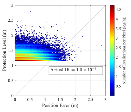
(a) Bayesian RAIM with fault exclusion

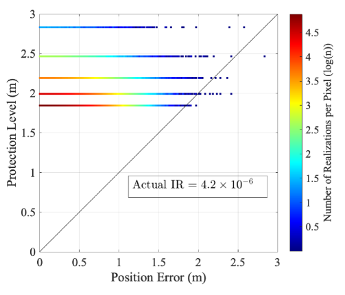
(b) Baseline RAIM

Figure 3: Stanford diagrams of the proposed Bayesian RAIM algorithm with fault exclusion in (a) and the baseline RAIM algorithm in (b). Plotted for $M=8$ and $\sigma_{n}=1$ over $5\times 10^{6}$ realizations, and with a $1$ cm $\times 1$ cm pixel size. A dot that appears on the bottom right side of the diagonal line represents an integrity failure (i.e., $|x-\hat{x}|>\mathrm{PL}$); the simulated IR of the Bayesian RAIM (a) is much tighter to the desired bound $\leq$ TIR ($10^{-3}$).

In each set of simulations, the simulated IR is obtained, that is, the ratio of realizations when the actual position error $|x-\hat{x}|$ exceeds the computed PLs among all realizations. It is found that the simulated IRs resultant from the Bayesian RAIM algorithms, with or without fault exclusion, all converged to the TIR after running enough realizations. This in turn proves that the posterior probabilities computed via the factor graph are exact. On the other hand, the simulated IR results of the baseline RAIM algorithm are in the order of $10^{-6}$, much lower than the TIR. For visualization, the results given by the Bayesian RAIM algorithm (with fault exclusion) and the baseline RAIM algorithm (also with fault exclusion) in the setting with $M=8$ BSs and $\sigma_{n}=1$ meter over $5\times 10^{6}$ realizations are presented in the form of Stanford diagram [8] in Fig. 3. As can be seen, the proposed Bayesian RAIM provides much tighter PLs while meeting the TIR requirement, compared to the baseline RAIM. The latter is conservative in PL computation, so the computed PLs are larger and the actual IR is significantly smaller than the TIR. One can also see that the PL results the baseline RAIM algorithms returns are discrete. This is because, unlike the Bayesian methods, the actual measurements are not utilized in the PL computation, as can be seen from (13). In particular, in (13), $N_{\mathrm{FM}}$ is determined by the number of measurements excluded, and $p_{\mathrm{FM},k}$, $T_{k}$ and $\sigma^{(k)}$ can only take a limited number of values, since the measurement models are assumed to be the same for all BSs.

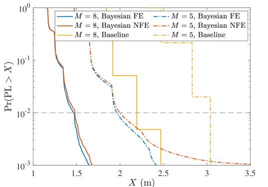
(a) $\sigma_{n}=1$ meter

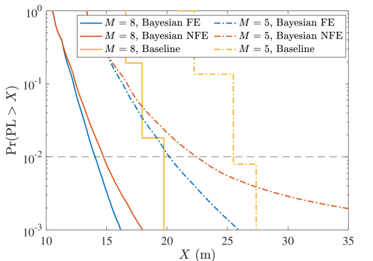
(b) $\sigma_{n}=9$ meters

Figure 4: CCDF curves of PLs under two values of the measurement noise level.

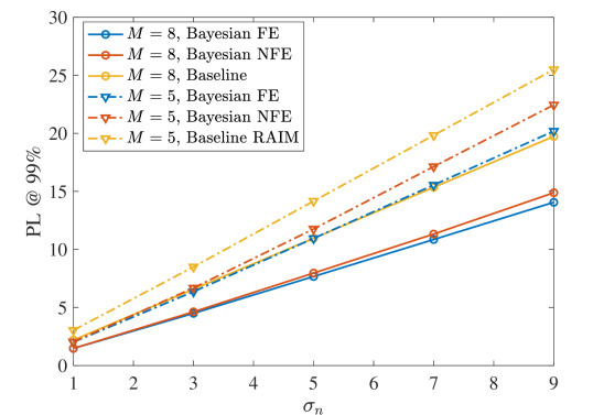
Figure 5: PL values at $99\%$ percentile as a function of the measurement noise level.

For each set of simulations, empirical complementary cumulative distribution function (CCDF) curves of the computed PLs are obtained. Four sets of the CCDF curves are presented in Fig. 4, from which the significant performance improvement of the proposed Bayesian RAIM algorithms over the baseline RAIM algorithm in obtaining tighter PLs can be clearly seen. In addition, the importance of fault exclusion before PL computation is revealed. Comparing the PL results given by the Bayesian RAIM algorithms with and without fault exclusion, we see that the large uncertainty introduced by the potentially faulty measurements in the posteriors leads to larger PL results (in a statistical sense), and the gap increases when $\sigma_{n}$ increases or/and when $M$ decreases, because the uncertainty can be reduced by providing more fault-free measurements or by reducing the measurement noises. To better illustrate this effect, in Fig. 5, the PL values at $99\%$ percentile (given by the intersections of the horizontal line at $10^{-2}$ with the CCDF curves) obtained under all sets of simulations are shown. Another interesting observation from Fig. 5 is that the $99\%$ percentile PL results given by any evaluated RAIM algorithms seem to increase linearly with $\sigma_{n}$.

VI Conclusion

A Bayesian RAIM algorithm has been developed for snapshot-type positioning problems under a 1D linear Gaussian setting, as a methodological validation. Position estimation, multi-fault detection and exclusion, and PL computation are performed based on the exact posterior distributions computed via message passing along a factor graph. It has been shown using Monte-Carlo simulation that the proposed algorithm provides tight PLs while satisfying the given TIR requirement, leading to a significant performance improvement over the baseline advanced RAIM algorithm. Encouraged by the result, the algorithm will be extended to the ToA-based 3D positioning problem under the same framework.

References

- [1] G. McKenzie, M. Hegarty, T. Barrett, and M. Goodchild, “Assessing the effectiveness of different visualizations for judgments of positional uncertainty,” Int. J. Geogr. Inf. Sci., vol. 30, no. 2, pp. 221–239, 2016.
- [2] T. Walter, P. Enge, and B. DeCleene, “Integrity lessons from the WAAS integrity performance panel (WIPP),” in Proc. ION NTM, 2003, pp. 183–194.
- [3] J. Blanch, T. Walker, P. Enge, Y. Lee, B. Pervan, M. Rippl, A. Spletter, and V. Kropp, “Baseline advanced RAIM user algorithm and possible improvements,” IEEE Trans. Aerosp. Electron. Syst., vol. 51, no. 1, pp. 713–732, 2015.
- [4] J. Marais, J. Beugin, and M. Berbineau, “A survey of GNSS-based research and developments for the european railway signaling,” IEEE Trans. Intell. Transp. Syst., vol. 18, no. 10, pp. 2602–2618, 2017.
- [5] T. G. Reid, S. E. Houts, R. Cammarata, G. Mills, S. Agarwal, A. Vora, and G. Pandey, “Localization requirements for autonomous vehicles,” SAE Int. J. Connected Autom. Veh., vol. 2, no. 12-02-03-0012, pp. 173–190, 2019.
- [6] J. Larson and D. Gebre-Egziabher, “Conservatism assessment of extreme value theory overbounds,” IEEE Trans. Aerosp. Electron. Syst., vol. 53, no. 3, pp. 1295–1307, 2017.
- [7] S. Dwivedi, R. Shreevastav, F. Munier, J. Nygren, I. Siomina, Y. Lyazidi, D. Shrestha, G. Lindmark, P. Ernström, E. Stare et al., “Positioning in 5G networks,” IEEE Commun. Mag., vol. 59, no. 11, pp. 38–44, 2021.
- [8] R. Whiton, “Cellular localization for autonomous driving: A function pull approach to safety-critical wireless localization,” IEEE Veh. Technol. Mag., vol. 17, no. 4, pp. 2–11, 2022.
- [9] M. Maaref and Z. M. Kassas, “Autonomous integrity monitoring for vehicular navigation with cellular signals of opportunity and an IMU,” IEEE Trans. Intell. Transp. Syst., 2021.
- [10] 3GPP, “Study on NR positioning enhancements,” 3rd Generation Partnership Project (3GPP), Technical Report (TR) 38.857, March 2021, version 17.0.0.
- [11] ——, “Study on expanded and improved NR positioning,” 3rd Generation Partnership Project (3GPP), Technical Report (TR) 38.859, Aug 2022, version 0.1.0.
- [12] N. Zhu, J. Marais, D. Bétaille, and M. Berbineau, “GNSS position integrity in urban environments: A review of literature,” IEEE Trans. Intell. Transp. Syst., vol. 19, no. 9, pp. 2762–2778, 2018.
- [13] H. Pesonen, “A framework for Bayesian receiver autonomous integrity monitoring in urban navigation,” Navigation, vol. 58, no. 3, pp. 229–240, 2011.
- [14] Q. Zhang and Q. Gui, “A new Bayesian RAIM for multiple faults detection and exclusion in GNSS,” J. Navig., vol. 68, no. 3, pp. 465–479, 2015.
- [15] S. Gupta and G. X. Gao, “Particle RAIM for integrity monitoring,” in Proc. 32nd ION GNSS, 2019, pp. 811–826.
- [16] J. Gabela, A. Kealy, M. Hedley, and B. Moran, “Case study of Bayesian RAIM algorithm integrated with spatial feature constraint and fault detection and exclusion algorithms for multi-sensor positioning,” Navigation, vol. 68, no. 2, pp. 333–351, 2021.
- [17] M. Koivisto, M. Costa, J. Werner, K. Heiska, J. Talvitie, K. Leppänen, V. Koivunen, and M. Valkama, “Joint device positioning and clock synchronization in 5G ultra-dense networks,” IEEE Trans. Wirel. Commun., vol. 16, no. 5, pp. 2866–2881, 2017.
- [18] I. Guvenc, S. Gezici, and Z. Sahinoglu, “Fundamental limits and improved algorithms for linear least-squares wireless position estimation,” Wirel. Commun. Mob. Comput., vol. 12, no. 12, pp. 1037–1052, 2012.
- [19] S. Zhu and Z. Ding, “A simple approach of range-based positioning with low computational complexity,” IEEE Trans. Wirel. Commun., vol. 8, no. 12, pp. 5832–5836, 2009.
- [20] F. R. Kschischang, B. J. Frey, and H.-A. Loeliger, “Factor graphs and the sum-product algorithm,” IEEE Trans. Inf. Theory, vol. 47, no. 2, pp. 498–519, 2001.