Field theories of active particle systems and their entropy production

Abstract

Active particles that translate chemical energy into self-propulsion can maintain a far-from-equilibrium steady state and perform work. The entropy production measures how far from equilibrium such a particle system operates and serves as a proxy for the work performed. Field theory offers a promising route to calculating entropy production, as it allows for many interacting particles to be considered simultaneously. Approximate field theories obtained by coarse-graining or smoothing that draw on additive noise can capture densities and correlations well, but they generally ignore the microscopic particle nature of the constituents, thereby producing spurious results for the entropy production. As an alternative we demonstrate how to use Doi-Peliti field theories, which capture the microscopic dynamics, including reactions and interactions with external and pair potentials. Such field theories are in principle exact, while offering a systematic approximation scheme, in the form of diagrammatics. We demonstrate how to construct them from a Fokker-Planck equation (FPE) of the single-particle dynamics and show how to calculate entropy production of active matter from first principles. This framework is easily extended to include interaction. We use it to derive exact, compact and efficient general expressions for the entropy production for a vast range of interacting particle systems. These expressions are independent of the underlying field theory and can be interpreted as the spatial average of the local entropy production. They are readily applicable to numerical and experimental data. In general, any pair interaction draws at most on the three point, equal time density and an $n$-point interaction on the $(2n-1)$-point density. We illustrate the technique in a number of exact, tractable examples, including some with pair-interaction.

I Introduction

Active matter has been the focus of much research in statistical mechanics and biophysics over the past decade, because of many surprising theoretical features Toner and Tu (1995); Cates (2012); Jülicher et al. (2018); Mandal et al. (2019), the rich phenomenology Cates and Tailleur (2015); Liebchen and Levis (2017) and a plethora of applications Di Leonardo et al. (2010); Xi et al. (2019); Pietzonka et al. (2019). At the heart of active matter lies the conversion of chemical fuel into mechanical work, often in the form of self-propulsion, which leads to sustained non-equilibrium behaviour that is distinctly different from that of relaxing equilibrium thermodynamic systems Cates (2012). How different, is quantified by the entropy production, which also quantifies the work performed. If we want to harvest and utilise this work, we need to quantify and control the system at the level it is observed and in the degrees of freedom that can be manipulated, rather than at a coarse-grained or smoothed level. The problem is illustrated by a team of horses observed from high above, when they may look almost like a droplet squeezing through a pore as they push past obstacles. At this level of description it may be difficult to distinguish a forward from a backward movie of the scene. Zooming in on the individual animal, however, reveals the details of their movement Muybridge (1878) and thus the difference between forward and backward immediately. If the horses are to be hitched to a plough, this is the level of observation needed to asses their utility. Assessing smoothed quasi-horses Mattuck (1992) does not help.

Field theory has been the work-horse of statistical mechanics for many decades Domb et al. (2001), because it allows for an efficient calculation and a systematic approximation of universal and non-universal observables in many-particle systems by means of a powerful machinery, that can be cast in an elegant, physically meaningful language in the form of diagrams. To apply this framework to active particle systems, effective field theories have been proposed, that use the continuously varying local particle density as the relevant degree of freedom. However, the entropy production of an approximating field theory is not necessarily a good approximation of the microscopic entropy production of the actual particle system. An exact, fully microscopic framework to calculate the entropy production systematically in active many-particle systems remains a theoretical challenge. In recent years, several exact results have been found Gaspard (2004), although those are limited to linear interaction forces Loos and Klapp (2020); Godrèche and Luck (2018), or cases where the full time-dependent particle probability density is known Cocconi et al. (2020).

The entropy production crucially depends on the degrees of freedom used to describe the system state. Coarse-graining by integrating out degrees of freedom or by mapping sets of microstates to mesostates generally underestimate the entropy production Roldán et al. (2021); Esposito (2012); Cocconi et al. (2022); Loos (2021). In Nardini et al. (2017) the particle dynamics has instead been approximated by recasting it as a continuously varying density subject to a Langevin equation of motion with additive noise. This approach captures much of the physics well, notably predicting that most of the entropy is produced at interfaces between dense and dilute phases Nardini et al. (2017); Martin et al. (2021); Fodor et al. (2022). Yet, it does not provide a lower bound of the entropy production, as it replaces the countably many particle degrees of freedom by the uncountably many of a density in space. Suppl. S-VI illustrates this in a simple, tractable example displaying a divergent entropy production.

Doi-Peliti field theories Doi (1976); Peliti (1985) on the other hand, retain the particle nature of the constituent degrees of freedom, but can be cumbersome to derive, normally requiring discretisation and an explicit derivation of a master equation. Instead, we demonstrate how a Doi-Peliti action can be determined using the Fokker-Planck operator governing the single particle dynamics. Interactions through external and pair potentials, as well as reactions can be added by virtue of the same Poissonian “superposition principle”, that allows a master equation to account for concurrent processes by adding corresponding gain and loss terms. We further show how the ensuing perturbation theory and its diagrammatics can be used to derive the entropy production, which turns out to draw only on the bare propagator and the lowest order perturbative vertices, as well as certain correlation functions. The diagrammatics of a field theory provides the small number of terms needed to calculate entropy production exactly. Our procedure results in very general formulae that need as system-specific input the details of the interaction potentials and a few low-order correlation functions. In the simplest case of non-interacting particles, the latter reduce to the one-point density, so that the entropy production becomes a spatial average of a local property. In general, if the interaction allows for up to $n$ particles interacting simultaneously, only the $(2n-1)$-point equal-time correlation function needs to be known, effectively quantifying where and how frequently such interactions take place. We thus introduce a generic scheme to derive tractable expressions for the entropy production of complex many-particle systems on the basis of their microscopic, stochastic equation of motion. We illustrate the technique in a number of examples.

The present work brings to bear the power of field theory to the field of active matter, while retaining particle entity, by calculating entropy production of the relevant degrees of freedom using diagrammatics and avoiding approximations altogether. Details of our derivations can be found in the supplemental material. We list the key results according to the structure of the article:

• Section II: We show how a Doi-Peliti field theory is readily derived from a Fokker-Planck Equation, in particular Eq. (4) from Eq. (1) (also Suppl. S-I).

• Section III: We introduce the framework to calculate entropy production, proceeding from the definition Eq. (8) via Eq. (12) to the diagrammatics of Eqs. (18) and (19) (also Suppl. .4 and Suppl. S-II).

• Section III.2: We include interaction, determining the relevant diagrams in Eq. (21), which immediately simplify to produce general expressions for $N$ pair-interacting indistinguishable particles such as Eq. (23) (also Suppl. S-V). A corresponding numerical scheme is readily derived as Eq. (24). We find that the entropy production of pair-interacting particles draws at most on the $3$-point density Lynn et al. (2022); Zhang and Garcia-Millan (2022a).

• Section IV: We give concrete examples: a Markov chain, drift-diffusion of a single particle (also Suppl. S-III), Eq. (IV), and two distinct particles on a circle (also Suppl. S-IV).

We conclude in Section V with a discussion, a summary of our results and an outlook.

II Field Theory from Fokker-Planck equation

An efficient way to characterise a many-particle system is in terms of occupation numbers, which allows for, in principle, arbitrary particle numbers and species without having to change the parameterisation, as opposed to a description in terms of the individual particle degrees of freedom. Doi-Peliti (DP) field theories provide a framework that readily caters for the spatio-temporal evolution of particles in terms of occupation numbers, in contrast to, say, the response field formalism Martin et al. (1973); Janssen (1976); de Dominicis (1976); Täuber (2014) which need correction terms in the form of Dean’s equation Dean (1996); Bothe et al. (2022). As the derivation of a DP field theory from a master equation can be cumbersome in particular in the presence of external fields Täuber et al. (2005); Cardy (2008), we demonstrate in Suppl. S-I that a DP field theory of non-interacting particles inherit the evolution operator of the one-particle Fokker-Planck equation (FPE). In particular, any continuum limit that has to be taken in a lattice-based master equation to derive the continuum FPE can equivalently be applied in the field theory. In other words, if the FPE of a density $\rho(\mathbf{y},t)$ reads

$$\partial_{t}\rho(\mathbf{y},t)=\operatorname*{\mathchoice{\ooalign{$\displaystyle\sum$\cr$\displaystyle\int$\cr}}{\ooalign{\raisebox{0.14pt}{{$\textstyle\sum$}}\cr$\textstyle\int$\cr}}{\ooalign{\raisebox{0.2pt}{{$\scriptstyle\sum$}}\cr$\scriptstyle\int$\cr}}{\ooalign{\raisebox{0.2pt}{{$\scriptstyle\sum$}}\cr$\scriptstyle\int$\cr}}}_{\mathbf{x}}\mathcal{L}_{\mathbf{y},\mathbf{x}}\rho(\mathbf{x},t)$$ (1)

with Fokker-Planck kernel $\mathcal{L}_{\mathbf{y},\mathbf{x}}$, then the Doi-Peliti action reads

$$\mathcal{A}_{0}=\int\mathchoice{\!\mathrm{d}t\,}{\!\mathrm{d}t\,}{\!\mathrm{d}t\,}{\!\mathrm{d}t\,}\operatorname*{\mathchoice{\ooalign{$\displaystyle\sum$\cr$\displaystyle\int$\cr}}{\ooalign{\raisebox{0.14pt}{{$\textstyle\sum$}}\cr$\textstyle\int$\cr}}{\ooalign{\raisebox{0.2pt}{{$\scriptstyle\sum$}}\cr$\scriptstyle\int$\cr}}{\ooalign{\raisebox{0.2pt}{{$\scriptstyle\sum$}}\cr$\scriptstyle\int$\cr}}}_{\mathbf{x},\mathbf{y}}\tilde{\phi}(\mathbf{y},t)(\mathcal{L}_{\mathbf{y},\mathbf{x}}-\delta(\mathbf{y}-\mathbf{x})\partial_{t})\phi(\mathbf{x},t)$$ (2)

with annihilator field $\phi(\mathbf{x},t)$, Doi-shifted creator field Cardy (2008) $\tilde{\phi}(\mathbf{y},t)$ and observables calculated in the path-integral Täuber et al. (2005); Täuber (2014)

$$\mathchoice{\left\langle\bullet\right\rangle_{0}}{\langle\bullet\rangle_{0}}{\langle\bullet\rangle_{0}}{\langle\bullet\rangle_{0}}=\int\mathcal{D}\!\phi\,\mathcal{D}\!\tilde{\phi}\,\mathchoice{e^{\mathcal{A}_{0}}}{\operatorname{exp}(\mathcal{A}_{0})}{\operatorname{exp}(\mathcal{A}_{0})}{\operatorname{exp}(\mathcal{A}_{0})}\bullet\ .$$ (3)

The simple relationship between Eqs. (1) and (2) is the first key-result of the present work. For continuous degrees of freedom, the kernel in Eq. (1) is usually written as $\mathcal{L}_{\mathbf{y},\mathbf{x}}=\hat{\mathcal{L}}^{\dagger}_{\mathbf{x}}\delta(\mathbf{x}-\mathbf{y})=\hat{\mathcal{L}}_{\mathbf{y}}\delta(\mathbf{x}-\mathbf{y})$ so that $\operatorname*{\mathchoice{\ooalign{$\displaystyle\sum$\cr$\displaystyle\int$\cr}}{\ooalign{\raisebox{0.14pt}{{$\textstyle\sum$}}\cr$\textstyle\int$\cr}}{\ooalign{\raisebox{0.2pt}{{$\scriptstyle\sum$}}\cr$\scriptstyle\int$\cr}}{\ooalign{\raisebox{0.2pt}{{$\scriptstyle\sum$}}\cr$\scriptstyle\int$\cr}}}_{\mathbf{x}}\mathcal{L}_{\mathbf{y},\mathbf{x}}\rho(\mathbf{x},t)=\hat{\mathcal{L}}_{\mathbf{y}}\rho(\mathbf{y},t)$ with FP operator $\hat{\mathcal{L}}_{\mathbf{y}}$ and $\hat{\mathcal{L}}^{\dagger}_{\mathbf{y}}$ its adjoint. In this case the action simplifies to

$$\mathcal{A}_{0}=\int\mathchoice{\!\mathrm{d}t\,}{\!\mathrm{d}t\,}{\!\mathrm{d}t\,}{\!\mathrm{d}t\,}\int\mathchoice{\!\mathrm{d}^{d}y\,}{\!\mathrm{d}^{d}y\,}{\!\mathrm{d}^{d}y\,}{\!\mathrm{d}^{d}y\,}\tilde{\phi}(\mathbf{y},t)(\hat{\mathcal{L}}_{\mathbf{y}}-\partial_{t})\phi(\mathbf{y},t).$$ (4)

The bare propagator

$$\mathchoice{\left\langle\phi(\mathbf{y},t^{\prime})\tilde{\phi}(\mathbf{x},t)\right\rangle_{0}}{\langle\phi(\mathbf{y},t^{\prime})\tilde{\phi}(\mathbf{x},t)\rangle_{0}}{\langle\phi(\mathbf{y},t^{\prime})\tilde{\phi}(\mathbf{x},t)\rangle_{0}}{\langle\phi(\mathbf{y},t^{\prime})\tilde{\phi}(\mathbf{x},t)\rangle_{0}}\triangleq\leavevmode\hbox to49.22pt{\vbox to16.92pt{\text{[drawing]}}} \mathbf{x},t \mathbf{y},t^{\prime} \mathbf{x},t \mathbf{y},t^{\prime}$$ (5)

of the action Eq. (2) is the Green function of the FPE (1), Suppl. S-I, and thus solves $\partial_{t^{\prime}}\mathchoice{\left\langle\phi(\mathbf{y},t^{\prime})\tilde{\phi}(\mathbf{x},t)\right\rangle_{0}}{\langle\phi(\mathbf{y},t^{\prime})\tilde{\phi}(\mathbf{x},t)\rangle_{0}}{\langle\phi(\mathbf{y},t^{\prime})\tilde{\phi}(\mathbf{x},t)\rangle_{0}}{\langle\phi(\mathbf{y},t^{\prime})\tilde{\phi}(\mathbf{x},t)\rangle_{0}}=\hat{\mathcal{L}}_{\mathbf{y}}\mathchoice{\left\langle\phi(\mathbf{y},t^{\prime})\tilde{\phi}(\mathbf{x},t)\right\rangle_{0}}{\langle\phi(\mathbf{y},t^{\prime})\tilde{\phi}(\mathbf{x},t)\rangle_{0}}{\langle\phi(\mathbf{y},t^{\prime})\tilde{\phi}(\mathbf{x},t)\rangle_{0}}{\langle\phi(\mathbf{y},t^{\prime})\tilde{\phi}(\mathbf{x},t)\rangle_{0}}$ with $\lim_{t^{\prime}\downarrow t}\mathchoice{\left\langle\phi(\mathbf{y},t^{\prime})\tilde{\phi}(\mathbf{x},t)\right\rangle_{0}}{\langle\phi(\mathbf{y},t^{\prime})\tilde{\phi}(\mathbf{x},t)\rangle_{0}}{\langle\phi(\mathbf{y},t^{\prime})\tilde{\phi}(\mathbf{x},t)\rangle_{0}}{\langle\phi(\mathbf{y},t^{\prime})\tilde{\phi}(\mathbf{x},t)\rangle_{0}}=\delta(\mathbf{y}-\mathbf{x})$.

The action Eq. (2) has by construction the same form as the action obtained by formally applying the MSR-trick Martin et al. (1973); Janssen (1976); de Dominicis (1976); Täuber (2014) to the FPE, despite the absence of a noise term. However, the DP field theory retains the particle nature of the constituent degrees of freedom without the need of additional terms, like Dean’s Dean (1996); Bothe et al. (2022). As a small price, a DP field theory is endowed with a commutator relation that needs to be consulted every time an observable is constructed from operators. As a consequence, unlike an effective Langevin-equation on the density, the annihilator field $\phi$ of a DP field theory is not the particle density Cardy (2008), and the action is not the particle density probability functional. Recasting the action in terms of a Langevin equation on the field $\phi$ can produce unexpected features, such as imaginary noise Howard and Täuber (1997); Lefevre and Biroli (2007). In a sense, the fields of a DP field theory are proxies, such that after expressing a desired observable in terms of fields according to the operators, the expectation of these fields is identical to that of the observable.

Drawing on the wealth of knowledge and intuition available for the construction of master equations, it is easy to incorporate into a DP field theory a wide range of terms, including reactions, transmutations, interactions, pair-potentials or external potentials, as the field theory’s action inherits the additivity of concurrent Poisson processes in a master equation. Some terms can be incorporated into the FP operator, others have to be treated perturbatively. Henceforth, we will assume that the full action

$$\mathcal{A}=\mathcal{A}_{0}+\mathcal{A}_{\text{pert}}$$ (6)

may contain perturbative terms such that expectations are calculated by expanding the exponential on the right hand side of

$$\mathchoice{\left\langle\bullet\right\rangle}{\langle\bullet\rangle}{\langle\bullet\rangle}{\langle\bullet\rangle}=\int\mathcal{D}\!\phi\,\mathcal{D}\!\tilde{\phi}\,\mathchoice{e^{\mathcal{A}}}{\operatorname{exp}(\mathcal{A})}{\operatorname{exp}(\mathcal{A})}{\operatorname{exp}(\mathcal{A})}\bullet=\mathchoice{\left\langle\ \bullet\ \operatorname{exp}\left(\mathcal{A}_{\text{pert}}\right)\right\rangle}{\langle\ \bullet\ \operatorname{exp}\left(\mathcal{A}_{\text{pert}}\right)\rangle}{\langle\ \bullet\ \operatorname{exp}\left(\mathcal{A}_{\text{pert}}\right)\rangle}{\langle\ \bullet\ \operatorname{exp}\left(\mathcal{A}_{\text{pert}}\right)\rangle}_{0}\ ,$$ (7)

and taking expectations as in Eq. (3). Even without interaction, $\mathcal{A}_{\text{pert}}$ may absorb terms of $\mathcal{L}$ that are not readily integrated in Eq. (3), so that the solution of the FPE (1) becomes in fact a perturbation theory. This is illustrated in Suppl. S-III for drift-diffusion in an arbitrary, periodic potential and in Garcia-Millan and Pruessner (2021) for Run-and-Tumble in a harmonic potential.

III Entropy production

In the present framework, the entropy production can be elegantly expressed in terms of the bare propagators and the perturbative part of the action. We will demonstrate this first for a single particle before generalising to multiple particles.

Following the scheme by Gaspard (Gaspard, 2004) to calculate entropy production in Markovian systems, we draw on the propagator $\mathchoice{\left\langle\phi(\mathbf{y},t^{\prime})\tilde{\phi}(\mathbf{x},t)\right\rangle}{\langle\phi(\mathbf{y},t^{\prime})\tilde{\phi}(\mathbf{x},t)\rangle}{\langle\phi(\mathbf{y},t^{\prime})\tilde{\phi}(\mathbf{x},t)\rangle}{\langle\phi(\mathbf{y},t^{\prime})\tilde{\phi}(\mathbf{x},t)\rangle}$ as the probability (density) for a particle to transition from $\mathbf{x}$ at time $t$ to $\mathbf{y}$ at time $t^{\prime}$. The internal entropy production of an evolving degree of freedom may then be written as a functional of the instantaneous probability (density) $\rho(\mathbf{x})$ to find it in state $\mathbf{x}$, namely

$$\dot{S}_{\text{int}}[\rho]=\operatorname*{\mathchoice{\ooalign{$\displaystyle\sum$\cr$\displaystyle\int$\cr}}{\ooalign{\raisebox{0.14pt}{{$\textstyle\sum$}}\cr$\textstyle\int$\cr}}{\ooalign{\raisebox{0.2pt}{{$\scriptstyle\sum$}}\cr$\scriptstyle\int$\cr}}{\ooalign{\raisebox{0.2pt}{{$\scriptstyle\sum$}}\cr$\scriptstyle\int$\cr}}}_{\mathbf{x},\mathbf{y}}\rho(\mathbf{x})\bm{\mathsf{K}}_{\mathbf{y},\mathbf{x}}\left\{\operatorname{\bm{\mathsf{Ln}}}_{\mathbf{y},\mathbf{x}}+\ln\left(\frac{\rho(\mathbf{x})}{\rho(\mathbf{y})}\right)\right\}$$ (8)

with

$$\bm{\mathsf{K}}_{\mathbf{y},\mathbf{x}}=\lim_{t^{\prime}\downarrow t}\frac{\mathrm{d}}{\mathrm{d}t^{\prime}}\mathchoice{\left\langle\phi(\mathbf{y},t^{\prime})\tilde{\phi}(\mathbf{x},t)\right\rangle}{\langle\phi(\mathbf{y},t^{\prime})\tilde{\phi}(\mathbf{x},t)\rangle}{\langle\phi(\mathbf{y},t^{\prime})\tilde{\phi}(\mathbf{x},t)\rangle}{\langle\phi(\mathbf{y},t^{\prime})\tilde{\phi}(\mathbf{x},t)\rangle}$$ (9)

and

$$\operatorname{\bm{\mathsf{Ln}}}_{\mathbf{y},\mathbf{x}}=\lim_{t^{\prime}\downarrow t}\ln\left(\frac{\mathchoice{\left\langle\phi(\mathbf{y},t^{\prime})\tilde{\phi}(\mathbf{x},t)\right\rangle}{\langle\phi(\mathbf{y},t^{\prime})\tilde{\phi}(\mathbf{x},t)\rangle}{\langle\phi(\mathbf{y},t^{\prime})\tilde{\phi}(\mathbf{x},t)\rangle}{\langle\phi(\mathbf{y},t^{\prime})\tilde{\phi}(\mathbf{x},t)\rangle}}{\mathchoice{\left\langle\phi(\mathbf{x},t^{\prime})\tilde{\phi}(\mathbf{y},t)\right\rangle}{\langle\phi(\mathbf{x},t^{\prime})\tilde{\phi}(\mathbf{y},t)\rangle}{\langle\phi(\mathbf{x},t^{\prime})\tilde{\phi}(\mathbf{y},t)\rangle}{\langle\phi(\mathbf{x},t^{\prime})\tilde{\phi}(\mathbf{y},t)\rangle}}\right)$$ (10)

as we show in Suppl. .4. Eq. (8) is the starting point for the derivation of the entropy production from a Doi-Peliti field theory. Much of what follows focuses on how to extract $\bm{\mathsf{K}}_{\mathbf{y},\mathbf{x}}$ and $\operatorname{\bm{\mathsf{Ln}}}_{\mathbf{y},\mathbf{x}}$ from the action.

As the field-theory correctly shows, Suppl. .4, if the states $\mathbf{y},\mathbf{x}$ are discrete and the process is a simple Markov chain, $\bm{\mathsf{K}}_{\mathbf{y},\mathbf{x}}$ reduces to the Markov (rate) matrix $\mathring{\mathcal{W}}_{\mathbf{y}\mathbf{x}}$ of the process of transitioning from $\mathbf{x}$ to $\mathbf{y}$, and $\operatorname{\bm{\mathsf{Ln}}}_{\mathbf{y},\mathbf{x}}$ is the logarithm of ratios of these rates,

$$\operatorname{\bm{\mathsf{Ln}}}_{\mathbf{y},\mathbf{x}}=\ln\left(\frac{\mathring{\mathcal{W}}_{\mathbf{y}\mathbf{x}}}{\mathring{\mathcal{W}}_{\mathbf{x}\mathbf{y}}}\right)\ ,$$ (11)

Eqs. (S-I.43) and (S-I.44c). If the states $\mathbf{x},\mathbf{y}$ are continuous, then $\bm{\mathsf{K}}_{\mathbf{y},\mathbf{x}}$ can be cast as a kernel, which in the absence of a perturbative contribution to the action is identical to the FP kernel, $\bm{\mathsf{K}}_{\mathbf{y},\mathbf{x}}=\mathcal{L}_{\mathbf{y},\mathbf{x}}$, given that the propagator is the Green function of the FPE, Suppl. .4. Integrating by parts then gives

$$\dot{S}_{\text{int}}[\rho]=\operatorname*{\mathchoice{\ooalign{$\displaystyle\sum$\cr$\displaystyle\int$\cr}}{\ooalign{\raisebox{0.14pt}{{$\textstyle\sum$}}\cr$\textstyle\int$\cr}}{\ooalign{\raisebox{0.2pt}{{$\scriptstyle\sum$}}\cr$\scriptstyle\int$\cr}}{\ooalign{\raisebox{0.2pt}{{$\scriptstyle\sum$}}\cr$\scriptstyle\int$\cr}}}_{\mathbf{x},\mathbf{y}}\rho(\mathbf{x})\delta(\mathbf{y}-\mathbf{x})\hat{\mathcal{L}}^{\dagger}_{\mathbf{y}}\left\{\operatorname{\bm{\mathsf{Ln}}}_{\mathbf{y},\mathbf{x}}+\ln\left(\frac{\rho(\mathbf{x})}{\rho(\mathbf{y})}\right)\right\}\ .$$ (12)

In principle, the density to use in Eqs. (8) and (12) is given by the propagation from the initial state up until time $t$, in which case it becomes an explicit function of $t$

$$\rho(\mathbf{x};t)=\mathchoice{\left\langle\phi(\mathbf{x},t)\tilde{\phi}(\mathbf{x}_{0},t_{0})\right\rangle}{\langle\phi(\mathbf{x},t)\tilde{\phi}(\mathbf{x}_{0},t_{0})\rangle}{\langle\phi(\mathbf{x},t)\tilde{\phi}(\mathbf{x}_{0},t_{0})\rangle}{\langle\phi(\mathbf{x},t)\tilde{\phi}(\mathbf{x}_{0},t_{0})\rangle}\ .$$ (13)

In general, this density might be well approximated by an effective theory, that omits the microscopic details entering into the entropy production via Eqs. (9) and (10).

The entropy production Eqs. (8) and (12) simplifies further if $\rho(\mathbf{x})$ is stationary,

$$\rho(\mathbf{x})=\operatorname*{\mathchoice{\ooalign{$\displaystyle\sum$\cr$\displaystyle\int$\cr}}{\ooalign{\raisebox{0.14pt}{{$\textstyle\sum$}}\cr$\textstyle\int$\cr}}{\ooalign{\raisebox{0.2pt}{{$\scriptstyle\sum$}}\cr$\scriptstyle\int$\cr}}{\ooalign{\raisebox{0.2pt}{{$\scriptstyle\sum$}}\cr$\scriptstyle\int$\cr}}}_{\mathbf{y}}\mathchoice{\left\langle\phi(\mathbf{x},t^{\prime})\tilde{\phi}(\mathbf{y},t)\right\rangle}{\langle\phi(\mathbf{x},t^{\prime})\tilde{\phi}(\mathbf{y},t)\rangle}{\langle\phi(\mathbf{x},t^{\prime})\tilde{\phi}(\mathbf{y},t)\rangle}{\langle\phi(\mathbf{x},t^{\prime})\tilde{\phi}(\mathbf{y},t)\rangle}\rho(\mathbf{y})$$ (14)

for any $t^{\prime}-t>0$, in which case $\ln(\rho(\mathbf{x})/\rho(\mathbf{y}))$ disappears from Eq. (8) and the expression reduces to that of the negative of the external entropy production Cocconi et al. (2020). In that case, Eq. (8) may be interpreted as the average $\dot{S}_{\text{int}}=\overline{\dot{\sigma}(\mathbf{x})}=\operatorname*{\mathchoice{\ooalign{$\displaystyle\sum$\cr$\displaystyle\int$\cr}}{\ooalign{\raisebox{0.14pt}{{$\textstyle\sum$}}\cr$\textstyle\int$\cr}}{\ooalign{\raisebox{0.2pt}{{$\scriptstyle\sum$}}\cr$\scriptstyle\int$\cr}}{\ooalign{\raisebox{0.2pt}{{$\scriptstyle\sum$}}\cr$\scriptstyle\int$\cr}}}_{\mathbf{x}}\rho(\mathbf{x})\dot{\sigma}(\mathbf{x})$ of the local entropy production

$$\dot{\sigma}(\mathbf{x})=\operatorname*{\mathchoice{\ooalign{$\displaystyle\sum$\cr$\displaystyle\int$\cr}}{\ooalign{\raisebox{0.14pt}{{$\textstyle\sum$}}\cr$\textstyle\int$\cr}}{\ooalign{\raisebox{0.2pt}{{$\scriptstyle\sum$}}\cr$\scriptstyle\int$\cr}}{\ooalign{\raisebox{0.2pt}{{$\scriptstyle\sum$}}\cr$\scriptstyle\int$\cr}}}_{\mathbf{y}}\bm{\mathsf{K}}_{\mathbf{y},\mathbf{x}}\operatorname{\bm{\mathsf{Ln}}}_{\mathbf{y},\mathbf{x}}\ ,$$ (15)

which derives from the dynamics only and is independent of the density. We will discuss the formalism in this form in greater detail below, after introducing interaction.

A priori, the full propagator is needed in Eqs. (9) and (10). However, as it turns out, provided the process is time-homogeneous, generally in the discrete case as well as in continuous perturbation theories about a Gaussian (details in Suppl. S-III), $\bm{\mathsf{K}}_{\mathbf{y},\mathbf{x}}$ and $\operatorname{\bm{\mathsf{Ln}}}_{\mathbf{y},\mathbf{x}}$ draw only on the bare propagator and possibly on the first order perturbative term. As detailed in Suppl. .4, the key argument for this simplification is that the propagator $\mathchoice{\left\langle\phi(\mathbf{y},t^{\prime})\tilde{\phi}(\mathbf{x},t)\right\rangle}{\langle\phi(\mathbf{y},t^{\prime})\tilde{\phi}(\mathbf{x},t)\rangle}{\langle\phi(\mathbf{y},t^{\prime})\tilde{\phi}(\mathbf{x},t)\rangle}{\langle\phi(\mathbf{y},t^{\prime})\tilde{\phi}(\mathbf{x},t)\rangle}$ only ever enters in the limit $t^{\prime}\downarrow t$, either in the form of an explicit derivative, Eq. (9), or in the form of a ratio, Eq. (10), which may also draw on the derivative via L’Hôpital. The propagator therefore needs to be determined only to first order in small $t^{\prime}-t$. If the full propagator $\mathchoice{\left\langle\phi(\mathbf{y},t^{\prime})\tilde{\phi}(\mathbf{x},t)\right\rangle}{\langle\phi(\mathbf{y},t^{\prime})\tilde{\phi}(\mathbf{x},t)\rangle}{\langle\phi(\mathbf{y},t^{\prime})\tilde{\phi}(\mathbf{x},t)\rangle}{\langle\phi(\mathbf{y},t^{\prime})\tilde{\phi}(\mathbf{x},t)\rangle}$ is given by a perturbative expansion of the action Eq. (7), diagrammatically written as

$$\mathchoice{\left\langle\phi(\mathbf{y},t^{\prime})\tilde{\phi}(\mathbf{x},t)\right\rangle}{\langle\phi(\mathbf{y},t^{\prime})\tilde{\phi}(\mathbf{x},t)\rangle}{\langle\phi(\mathbf{y},t^{\prime})\tilde{\phi}(\mathbf{x},t)\rangle}{\langle\phi(\mathbf{y},t^{\prime})\tilde{\phi}(\mathbf{x},t)\rangle}\triangleq\leavevmode\hbox to49.22pt{\vbox to16.92pt{\text{[drawing]}}}+\leavevmode\hbox to60.6pt{\vbox to18.87pt{\text{[drawing]}}}+\leavevmode\hbox to80.52pt{\vbox to18.87pt{\text{[drawing]}}}+\ldots\ , \mathbf{x},t \mathbf{y},t^{\prime} \mathbf{x},t \mathbf{y},t^{\prime} \mathbf{x},t \mathbf{y},t^{\prime} \mathbf{x},t \mathbf{y},t^{\prime} \mathbf{x},t \mathbf{y},t^{\prime} \mathbf{x},t \mathbf{y},t^{\prime}$$ (16)

in principle every order in the perturbation theory might contribute to $\mathchoice{\left\langle\phi(\mathbf{y},t^{\prime})\tilde{\phi}(\mathbf{x},t)\right\rangle}{\langle\phi(\mathbf{y},t^{\prime})\tilde{\phi}(\mathbf{x},t)\rangle}{\langle\phi(\mathbf{y},t^{\prime})\tilde{\phi}(\mathbf{x},t)\rangle}{\langle\phi(\mathbf{y},t^{\prime})\tilde{\phi}(\mathbf{x},t)\rangle}$ to first order in $t^{\prime}-t$. As outlined in the following, closer inspection, however, reveals a simple relationship, namely that the $n$th order in $t^{\prime}-t$ is fully given by the first $n$ diagrams on the right hand side of Eq. (16). In continuum field theories, this needs careful analysis, but it holds for perturbation theories about drift-diffusion, Suppl. S-III, where the highest order derivative in $\bm{\mathsf{K}}_{\mathbf{y},\mathbf{x}}$ is a second and $\operatorname{\bm{\mathsf{Ln}}}_{\mathbf{y},\mathbf{x}}$, necessarily odd in $\mathbf{y}-\mathbf{x}$, therefore does not need to be known beyond second order.

Leaving the details to the supplement Suppl. .4 and Suppl. S-II, we proceed by demonstrating that the first time derivative of the second order contribution on the right hand side of Eq. (16) vanishes at $t^{\prime}=t$. This follows from differentiating with respect to $t^{\prime}$ the inverse Fourier-transform of , which for time-homogeneous processes has the form

$$\dot{I}(t^{\prime}-t)=\int\mathchoice{\!\text{\dj}\omega^{\prime}\,}{\!\text{\dj}\omega^{\prime}\,}{\!\text{\dj}\omega^{\prime}\,}{\!\text{\dj}\omega^{\prime}\,}\frac{-\mathring{\imath}\omega^{\prime}\mathchoice{e^{-\mathring{\imath}\omega^{\prime}(t^{\prime}-t)}}{\operatorname{exp}(-\mathring{\imath}\omega^{\prime}(t^{\prime}-t))}{\operatorname{exp}(-\mathring{\imath}\omega^{\prime}(t^{\prime}-t))}{\operatorname{exp}(-\mathring{\imath}\omega^{\prime}(t^{\prime}-t))}C}{\prod_{j=1}^{3}(-\mathring{\imath}\omega^{\prime}+p_{j})}\ ,$$ (17)

where the three propagators are $(-\mathring{\imath}\omega^{\prime}+p_{j})^{-1}$ with $j=1,2,3$ and $C$ denotes the couplings. The poles $-\mathring{\imath}p_{j}$ may be repeated, which does not affect the argument. Crucially, all poles are situated in the lower half-plane, which is required by causality of each bare propagator entering in Eq. (17). After taking $t^{\prime}\to t$ the contour can be closed in the upper half-plane, as the integrand $\propto 1/\omega^{\prime 2}$ decays fast enough. It follows that $\dot{I}(0)$, Eq. (17), vanishes. This argument easily generalises to higher derivatives and correspondingly higher orders. Consequently, only the first two diagrams on the right hand side of Eq. (16) contribute to the propagator to first order in $t^{\prime}-t$.

The argument above draws on the structure of the diagrams where bare propagators connect “blobs”. The diagrams in the propagators of Eqs. (9) and (10) that end up contributing, contain at most one such blob. How the blob enters into $\bm{\mathsf{K}}_{\mathbf{y},\mathbf{x}}$ and $\operatorname{\bm{\mathsf{Ln}}}_{\mathbf{y},\mathbf{x}}$ is explained in the following. The blobs can contain tadpole-like loops only in the presence of source terms, such as Eq. (S-II.11). If such source terms are absent, the blobs are merely the vertices of the perturbative part of the action. If the phenomenon studied is not time-homogeneous, $\omega$ might have sinks and sources and the structure of the integrals representing contributions to the propagator are no longer of the form Eq. (17).

With these provisos in place, the kernel needed in Eq. (9) reduces to the bare propagator plus the first order correction,

$$\bm{\mathsf{K}}_{\mathbf{y},\mathbf{x}}\triangleq\mathcal{L}_{\mathbf{y},\mathbf{x}}+\leavevmode\hbox to29.02pt{\vbox to16.55pt{\text{[drawing]}}}\ , \mathbf{x} \mathbf{y} \mathbf{x} \mathbf{y}$$ (18)

where $\mathcal{L}$ refers to the non-perturbative part of the action Eq. (2), and to the first order, one-particle irreducible, amputated contributions due to the perturbative part of the action, the “blob”. It may contain perturbative contributions due to the single-particle Fokker-Planck operator, or due to additional processes, such as interactions and reactions. In field-theoretic terms, $\mathcal{L}_{\mathbf{y},\mathbf{x}}$ is the inverse bare propagator evaluated at $\omega=0$ and is a contribution to the ”self-energy”. In stochastic particle systems, $\mathcal{L}_{\mathbf{y},\mathbf{x}}=(D\partial_{y}^{2}-w\partial_{y})\delta(y-x)$ would be drift-diffusion (Suppl. S-III) and $\leavevmode\hbox to15.2pt{\vbox to9.22pt{\text{[drawing]}}}=-r$ an additional extinction with rate $r$. Generally, no higher orders, such as , or any loops carrying $\omega$, such as the middle term in Eq. (22), enter (Suppl. S-II). While maybe unsurprising as far as the kernel $\bm{\mathsf{K}}_{\mathbf{y},\mathbf{x}}$ is concerned, this simplification to one blob carries through to the logarithm on the basis of Eqs. (11) and (S-I.47) if states are discrete, and by an expansion of the form

$$\operatorname{\bm{\mathsf{Ln}}}_{\mathbf{y},\mathbf{x}}\triangleq\lim_{t^{\prime}\downarrow t}\left\{\ln\left(\frac{\leavevmode\hbox to49.22pt{\vbox to16.92pt{\text{[drawing]}}}}{\leavevmode\hbox to49.22pt{\vbox to16.92pt{\text{[drawing]}}}}\right)+\frac{\leavevmode\hbox to60.6pt{\vbox to18.87pt{\text{[drawing]}}}}{\leavevmode\hbox to49.22pt{\vbox to16.92pt{\text{[drawing]}}}}-\frac{\leavevmode\hbox to60.6pt{\vbox to18.87pt{\text{[drawing]}}}}{\leavevmode\hbox to49.22pt{\vbox to16.92pt{\text{[drawing]}}}}\right\}\ , \mathbf{x},t \mathbf{y},t^{\prime} \mathbf{y},t \mathbf{x},t^{\prime} \mathbf{x},t \mathbf{y},t^{\prime} \mathbf{x},t \mathbf{y},t^{\prime} \mathbf{y},t \mathbf{x},t^{\prime} \mathbf{y},t \mathbf{x},t^{\prime} \mathbf{x},t \mathbf{y},t^{\prime} \mathbf{y},t \mathbf{x},t^{\prime} \mathbf{x},t \mathbf{y},t^{\prime} \mathbf{x},t \mathbf{y},t^{\prime} \mathbf{y},t \mathbf{x},t^{\prime} \mathbf{y},t \mathbf{x},t^{\prime}$$ (19)

in the continuum, Eq. (S-I.54) and similarly Suppl. S-III, Eq. (S-III.32).

In summary, what is needed to calculate the entropy production Eq. (8) of a single degree of freedom is: (a) the density $\rho(\mathbf{x};t)$, which at stationarity may be well approximated by an effective theory, and (b) the microscopic action Eq. (6) to construct kernel $\bm{\mathsf{K}}_{\mathbf{y},\mathbf{x}}$, via Eq. (18), and logarithm $\operatorname{\bm{\mathsf{Ln}}}_{\mathbf{y},\mathbf{x}}$ via Eq. (19) using at most one blob.

III.1 Many conserved particles

In the presence of $N>1$ distinguishable particles, Eq. (8) remains in principle valid if $\mathbf{x},\mathbf{y}$ are understood to encapsulate all $N$ particle coordinates at once, with the density in Eq. (8) replaced by the joint density $\rho(\mathbf{x}_{1},\ldots,\mathbf{x}_{N})$ and the propagator in Eqs. (9) and (10) replaced by the joint propagator $\bigl{\langle}\phi_{1}(\mathbf{y}_{1},t^{\prime})\linebreak[1]\phi_{2}(\mathbf{y}_{2},t^{\prime})\linebreak[1]\ldots\linebreak[1]\phi_{N}(\mathbf{y}_{N},t^{\prime})\linebreak[1]\tilde{\phi}_{1}(\mathbf{x}_{1},t)\linebreak[1]\tilde{\phi}_{2}(\mathbf{x}_{2},t)\linebreak[1]\ldots\linebreak[1]\tilde{\phi}_{N}(\mathbf{x}_{N},t)\bigr{\rangle}$, where the indices of the fields refer to distinguishable particle species. Without interaction, the overall entropy production is the sum of the individual entropy productions, Eq. (S-V.41). If particles are indistinguishable, dropping the indices generally results in $N!$ as many terms from permutations of the fields, as well as the joint density $\rho(\mathbf{x}_{1},\ldots,\mathbf{x}_{N})$ at stationarity being $N!$ that of distinguishable particles. At the same time, the phase space summed or integrated over in Eq. (8) has to be adjusted to reflect that occupation numbers are the degrees of freedom, not particle positions Cocconi et al. (2020); Zhang and Garcia-Millan (2022a). In the case of sparse occupation, where every site is occupied by at most one particle, a condition usually met in continuum space, this can be done by means of the Gibbs factor Sethna (2006), which amounts to dividing the phase space of distinguishable particles by $N!$,

$$\dot{S}_{\text{int}}^{(N)}[\rho]=\frac{1}{(N!)^{2}}\int\mathchoice{\!\mathrm{d}^{d}x_{1}\,}{\!\mathrm{d}^{d}x_{1}\,}{\!\mathrm{d}^{d}x_{1}\,}{\!\mathrm{d}^{d}x_{1}\,}\ldots\mathchoice{\!\mathrm{d}^{d}x_{N}\,}{\!\mathrm{d}^{d}x_{N}\,}{\!\mathrm{d}^{d}x_{N}\,}{\!\mathrm{d}^{d}x_{N}\,}\int\mathchoice{\!\mathrm{d}^{d}y_{1}\,}{\!\mathrm{d}^{d}y_{1}\,}{\!\mathrm{d}^{d}y_{1}\,}{\!\mathrm{d}^{d}y_{1}\,}\ldots\mathchoice{\!\mathrm{d}^{d}y_{N}\,}{\!\mathrm{d}^{d}y_{N}\,}{\!\mathrm{d}^{d}y_{N}\,}{\!\mathrm{d}^{d}y_{N}\,}\rho^{(N)}(\mathbf{x}_{1},\ldots,\mathbf{x}_{N})\bm{\mathsf{K}}^{(N)}_{\mathbf{y}_{1},\ldots,\mathbf{y}_{N},\mathbf{x}_{1},\ldots,\mathbf{x}_{N}}\operatorname{\bm{\mathsf{Ln}}}^{(N)}_{\mathbf{y}_{1},\ldots,\mathbf{y}_{N},\mathbf{x}_{1},\ldots,\mathbf{x}_{N}}$$ (20)

with $N$-particle kernel $\bm{\mathsf{K}}^{(N)}_{\mathbf{y}_{1},\ldots,\mathbf{x}_{N}}$ and logarithm $\operatorname{\bm{\mathsf{Ln}}}^{(N)}_{\mathbf{y}_{1},\ldots,\mathbf{x}_{N}}$ defined by using the joint propagator $\bigl{\langle}\phi(\mathbf{y}_{1},t^{\prime})\linebreak[1]\ldots\linebreak[1]\tilde{\phi}(\mathbf{x}_{N},t)\bigr{\rangle}$ on the right of Eqs. (9) and (10). At stationarity, the Gibbs factor precisely cancels the multiplicity of the terms mentioned above, Suppl. .1. Again, without interaction, the entropy production of $N$ indistinguishable particles is linear in $N$, Eq. (S-V.98).

The diagrams contributing to the joint propagator are generally disconnected, say and may, in principle, involve any number of vertices, such as , say or . However, as detailed in Suppl. S-II, the argument that reduces to at most one vertex contributions to a single particle propagator, similarly applies to multiple particle propagators, so that any blob inside a joint propagator raises the order of $t^{\prime}-t$ by one. Any contribution to the joint propagator $\bigl{\langle}\phi(\mathbf{y}_{1},t)\linebreak[1]\ldots\linebreak[1]\tilde{\phi}(\mathbf{x}_{N},t)\bigr{\rangle}$ in the joint kernel $\bm{\mathsf{K}}_{\mathbf{y}_{1},\ldots,\mathbf{x}_{N}}$ or the joint logarithm $\operatorname{\bm{\mathsf{Ln}}}_{\mathbf{y}_{1},\ldots,\mathbf{x}_{N}}$ therefore contains at most one vertex. The set of diagrams to be considered can be reduced further with an argument best made after allowing for interaction.

III.2 Interaction

In the presence of interaction, the joint propagator contains contributions of the form . Each such vertex is also of order $t^{\prime}-t$, Suppl. S-II. If particles are conserved, each vertex must have at least as many incoming legs as outgoing ones. At this stage, the joint propagator entering the $N$ particle kernel $\bm{\mathsf{K}}^{(N)}$ and logarithm $\operatorname{\bm{\mathsf{Ln}}}^{(N)}$ is of the form

$$\mathchoice{\left\langle\phi(\mathbf{y}_{1},t^{\prime})\ldots\phi(\mathbf{y}_{N},t^{\prime})\tilde{\phi}(\mathbf{x}_{1},t)\ldots\tilde{\phi}(\mathbf{x}_{N},t)\right\rangle}{\langle\phi(\mathbf{y}_{1},t^{\prime})\ldots\phi(\mathbf{y}_{N},t^{\prime})\tilde{\phi}(\mathbf{x}_{1},t)\ldots\tilde{\phi}(\mathbf{x}_{N},t)\rangle}{\langle\phi(\mathbf{y}_{1},t^{\prime})\ldots\phi(\mathbf{y}_{N},t^{\prime})\tilde{\phi}(\mathbf{x}_{1},t)\ldots\tilde{\phi}(\mathbf{x}_{N},t)\rangle}{\langle\phi(\mathbf{y}_{1},t^{\prime})\ldots\phi(\mathbf{y}_{N},t^{\prime})\tilde{\phi}(\mathbf{x}_{1},t)\ldots\tilde{\phi}(\mathbf{x}_{N},t)\rangle}\\ \triangleq\leavevmode\hbox to80.61pt{\vbox to43.35pt{\text{[drawing]}}}+\text{perm.}+\leavevmode\hbox to80.61pt{\vbox to43.35pt{\text{[drawing]}}}+\text{perm.}+\leavevmode\hbox to80.61pt{\vbox to43.35pt{\text{[drawing]}}}+\text{perm.}+\mathcal{O}\left((t^{\prime}-t)^{2}\right)\ , \mathbf{x}_{1},t \mathbf{y}_{1},t^{\prime} \mathbf{x}_{2},t \mathbf{y}_{2},t^{\prime} \vdots \mathbf{x}_{N},t \mathbf{y}_{N},t^{\prime} \mathbf{x}_{1},t \mathbf{y}_{1},t^{\prime} \mathbf{x}_{2},t \mathbf{y}_{2},t^{\prime} \vdots \mathbf{x}_{N},t \mathbf{y}_{N},t^{\prime} \mathbf{x}_{1},t \mathbf{y}_{1},t^{\prime} \mathbf{x}_{2},t \mathbf{y}_{2},t^{\prime} \vdots \mathbf{x}_{N},t \mathbf{y}_{N},t^{\prime} \mathbf{x}_{1},t \mathbf{y}_{1},t^{\prime} \mathbf{x}_{2},t \mathbf{y}_{2},t^{\prime} \vdots \mathbf{x}_{N},t \mathbf{y}_{N},t^{\prime} \mathbf{x}_{1},t \mathbf{y}_{1},t^{\prime} \mathbf{x}_{2},t \mathbf{y}_{2},t^{\prime} \vdots \mathbf{x}_{N},t \mathbf{y}_{N},t^{\prime} \mathbf{x}_{1},t \mathbf{y}_{1},t^{\prime} \mathbf{x}_{2},t \mathbf{y}_{2},t^{\prime} \vdots \mathbf{x}_{N},t \mathbf{y}_{N},t^{\prime}$$ (21)

each with all distinct permutations of incoming and outgoing particle coordinates, $\mathbf{x}_{i}$ and $\mathbf{y}_{i}$ respectively, as indicated by perm.. What does not enter (Suppl. S-II) are terms involving more than one vertex, such as

$$\leavevmode\hbox to40.63pt{\vbox to35.47pt{\text{[drawing]}}}\,\text{ or }\,\leavevmode\hbox to40.63pt{\vbox to33.32pt{\text{[drawing]}}}\,\text{ or }\,\leavevmode\hbox to40.63pt{\vbox to31.21pt{\text{[drawing]}}}\ . \vdots \vdots \vdots \vdots \vdots \vdots$$ (22)

Even with the restriction to a single blob, Eq. (21) contains many diagrams, seemingly involving many permutations of many initial and final coordinates. Similarly, the $N$-point equal time density $\rho^{(N)}(\mathbf{x}_{1},\ldots,\mathbf{x}_{N})$ is needed in Eq. (20), which would be an ardeous task to determine. However, because every bare propagator degenerates into a $\delta$-function as $t^{\prime}\downarrow t$, they can considerably simplify the expression for the entropy production. As discussed in Suppl. S-V any bare propagator featuring together with, i.e. multiplying, a blobbed diagram, effectively drops out in the limit $t^{\prime}\downarrow t$. As the bare propagators drop away, so does the need for higher order densities. As a result the entropy production of a system whose ”largest blob” has $n$ incoming and $n$ outgoing legs can be calculated on the basis of the $(2n-1)$-point joint density, restricting a hierarchy of terms to $2n-1$ rather than $N$ Lynn et al. (2022).

For example, $N$ indistinguishable particles with self-propulsion speed $\mathbf{w}$, diffusion $D$ and pair-interaction, $n=2$, via an even potential $U$ have entropy production,

$$\dot{S}_{\text{int}}^{(N)}[\rho^{(N)}]= \int\mathchoice{\!\mathrm{d}^{d}\mathbf{x}_{1}\,}{\!\mathrm{d}^{d}\mathbf{x}_{1}\,}{\!\mathrm{d}^{d}\mathbf{x}_{1}\,}{\!\mathrm{d}^{d}\mathbf{x}_{1}\,}\rho_{1}^{(N)}(\mathbf{x}_{1})\left\{\frac{\mathbf{w}^{2}}{D}\right\}$$ (23a)

$$+\int\mathchoice{\!\mathrm{d}^{d}\mathbf{x}_{1,2}\,}{\!\mathrm{d}^{d}\mathbf{x}_{1,2}\,}{\!\mathrm{d}^{d}\mathbf{x}_{1,2}\,}{\!\mathrm{d}^{d}\mathbf{x}_{1,2}\,}\rho_{2}^{(N)}(\mathbf{x}_{1},\mathbf{x}_{2})\left\{\frac{1}{D}\left(\nabla U(\mathbf{x}_{1}-\mathbf{x}_{2})\right)^{2}-\mathop{}\!\mathbin{\bigtriangleup}U(\mathbf{x}_{1}-\mathbf{x}_{2})\right\}$$ (23b)

$$+\int\mathchoice{\!\mathrm{d}^{d}\mathbf{x}_{1,2,3}\,}{\!\mathrm{d}^{d}\mathbf{x}_{1,2,3}\,}{\!\mathrm{d}^{d}\mathbf{x}_{1,2,3}\,}{\!\mathrm{d}^{d}\mathbf{x}_{1,2,3}\,}\rho_{3}^{(N)}(\mathbf{x}_{1},\mathbf{x}_{2},\mathbf{x}_{3})\left\{\frac{1}{D}\nabla U(\mathbf{x}_{1}-\mathbf{x}_{2})\cdot\nabla U(\mathbf{x}_{1}-\mathbf{x}_{3})\right\}\ ,$$ (23c)

which is Eq. (S-V.109) with external potential $\Upsilon\equiv 0$ and further simplified by using that the pair potential $U$ is even. It demonstrably vanishes in the absence of drift $\mathbf{w}$, as shown in Suppl. .2. Eq. (23) and (S-V.109) are exact results, assuming pair interaction being the highest order interaction as well as sparse occupation, which here means merely that two particles cannot be located at exactly the same point in space, something that in the continuum is practically always fulfilled. The densities $\rho_{n}^{(N)}(\mathbf{x}_{1},\ldots,\mathbf{x}_{n})$ thus denote the density of $n$ distinct particles at positions $\mathbf{x}_{1},\ldots\mathbf{x}_{n}$, normalising to $N!/(N-n)!$. Each term in curly brackets in Eq. (23) can be cast as a local entropy production, depending on one, two or three coordinates. Eq. (23a) is the entropy production or work due to self-propulsion by individual particles, $N\mathbf{w}^{2}/D$, Eq. (23b) is the work due to two particles excerting equal and opposite forces on each other and Eq. (23c) is the work performed by one particle in the potential of another particle as it is being pushed or pulled by a third particle.

In the form of Eq. (23), entropy production in an experiment or simulation can be estimated efficiently by using $Q$ samples $q=1,2,\ldots,Q$ of $N$ particle coordinates $\mathbf{x}^{(q)}_{i}$ with $i=1,\ldots,N$,

$$\dot{S}_{\text{int}}=\frac{1}{Q}\sum_{q=1}^{Q}\left[\sum_{i_{1}=1}^{N}\dot{\sigma}^{(1)}_{1}\left(\mathbf{x}^{(q)}_{i_{1}}\right)+\sum_{i_{1},i_{2}=1\atop i_{1}\neq i_{2}}^{N}\dot{\sigma}^{(2)}_{2}\left(\mathbf{x}^{(q)}_{i_{1}},\mathbf{x}^{(q)}_{i_{2}}\right)+\sum_{i_{1},i_{2}=1\atop i_{1}\neq i_{2}\neq i_{3}\neq i_{1}}^{N}\dot{\sigma}^{(3)}_{3}\left(\mathbf{x}^{(q)}_{i_{1}},\mathbf{x}^{(q)}_{i_{2}},\mathbf{x}^{(q)}_{i_{1}}\right)\right]\ .$$ (24)

with the $\dot{\sigma}^{(i)}_{i}$ with $i=1,2,3$ given by the three pairs of curly brackets in Eq. (23) and generally in Eq. (S-V.104). All sums run over distinct particle indices, so that for example $(1/Q)\sum_{q}\sum_{i_{1},i_{2}=1\atop i_{1}\neq i_{2}}^{N}\delta(\mathbf{x}_{1}-\mathbf{x}^{(q)}_{i_{1}})\delta(\mathbf{x}_{2}-\mathbf{x}^{(q)}_{i_{2}})$ estimates $\rho_{2}^{(N)}(\mathbf{x}_{1},\mathbf{x}_{2})$. Entropy production in a particle system with interaction can thus be estimated on the basis of ”snapshots” and the microscopic action, without the need of introducing a new measure Ro et al. (2021); Tociu et al. (2020). In the case of $n$-particle interaction, it generally draws on equal-time $(2n-1)$-point densities and the time-evolution terms given by the action. Neither the full $N$-point density nor the $2N$-point two-time correlation function is needed, which is what Eq. (20) suggests.

If the number of particles is not fixed but becomes itself a degree of freedom, the phase space integrated or summed over in Eq. (8) needs to be adjusted. This case is beyond the scope of the present work.

IV Examples

In the following we illustrate the methods introduced above by calculating the entropy production of 1) a continuous time Markov chain, 2) a drift-diffusion Brownian particle on a torus with potential, and 3) two drift-diffusion particles on a circle interacting via a harmonic pair potential.

Continuous time Markov chain.

The single-particle master equation of a continuous time Markov chain is Eq. (1) with $\mathcal{L}_{\mathbf{y}\mathbf{x}}$ the Markov-matrix $\mathcal{M}_{\mathbf{y}\mathbf{x}}$ for transitions from discrete state $\mathbf{x}$ to $\mathbf{y}$. Following standard procedure Täuber et al. (2005), Suppl. S-I, the action of the resulting field theory is Eq. (2),

$$\mathcal{A}_{0}=\sum_{\mathbf{x}\mathbf{y}}\mathchoice{\!\mathrm{d}t\,}{\!\mathrm{d}t\,}{\!\mathrm{d}t\,}{\!\mathrm{d}t\,}\tilde{\phi}(\mathbf{y},t)(\mathcal{M}_{\mathbf{y}\mathbf{x}}-\delta_{\mathbf{y},\mathbf{x}}\partial_{t})\phi(\mathbf{x},t)\ .$$ (25)

From Eqs. (8), (11) and (18) in the absence of a perturbative term, the entropy production immediately follows,

$$\dot{S}_{\text{int}}[\rho]=\sum_{\mathbf{x},\mathbf{y}}\mathcal{M}_{\mathbf{y}\mathbf{x}}\rho(\mathbf{x})\ln\left(\frac{\mathcal{M}_{\mathbf{y}\mathbf{x}}\rho(\mathbf{x})}{\mathcal{M}_{\mathbf{x}\mathbf{y}}\rho(\mathbf{y})}\right)\ ,$$ (26)

Suppl. .1, consistent with Gaspard (2004); Cocconi et al. (2020). The contributions to first order in the perturbative vertex in Eqs. (18), (S-I.46a) and (S-I.47) ensure that this expression for the entropy production does not change even when some contributions to $\mathcal{M}$ are moved to the perturbative part of the action, $\mathcal{B}$ in Eqs. (S-I.46a) and (S-I.47).

Drift-diffusion.

This process is a paradigmatic example of a continuous space process as many other, more complicated ones, in particular many active matter models Zhang and Pruessner (2022); Zhang et al. (2022); Zhen and Pruessner (2022) can be studied as a perturbation of it. The continuity of the degree of freedom means that a transform is needed to render the process local in a new variable, here the Fourier-mode $\mathbf{k}$, so that the path-integral Eq. (7) can be performed. However, as detailed in Suppl. S-III, the transform can in principle spoil the relationship between the number of blobs in the diagram and its order in $t^{\prime}-t$ as discussed around Eq. (17). It turns out, Suppl. .1, that in the case of drift-diffusion processes, the number of blobs determines the leading order in the distance $\mathbf{y}-\mathbf{x}$ of any contribution finite in the limit $t^{\prime}\downarrow t$, in fact preserving Eqs. (18) and (19).

To be general, we allow for an external potential, but to render drift diffusion stationary even without an external potential, we restrict it to a $d$-dimensional torus of circumference $L$. As detailed in Suppl. S-III, the drift can be captured either exactly or perturbatively, while an external potential generally has to be treated perturbatively. The FPE of a particle diffusing with constant $D$ and drifting with velocity $\mathbf{w}$ on a torus with periodic external potential $\Upsilon(\mathbf{y})$ is Eq. (1) with $\hat{\mathcal{L}}_{\mathbf{y}}=D\nabla_{\mathbf{y}}^{2}+\nabla_{\mathbf{y}}(-\mathbf{w}+\Upsilon^{\prime}(\mathbf{y}))$, where the operators act on everything to the right and $\Upsilon^{\prime}=\nabla\Upsilon$ denotes the gradient of the potential. The propagator to first order is (Suppl. S-III, Eqs. (S-III.36))

$$\mathchoice{\left\langle\phi(\mathbf{y},t^{\prime})\tilde{\phi}(\mathbf{x},t)\right\rangle}{\langle\phi(\mathbf{y},t^{\prime})\tilde{\phi}(\mathbf{x},t)\rangle}{\langle\phi(\mathbf{y},t^{\prime})\tilde{\phi}(\mathbf{x},t)\rangle}{\langle\phi(\mathbf{y},t^{\prime})\tilde{\phi}(\mathbf{x},t)\rangle}= \frac{\theta(t^{\prime}-t)\mathchoice{e^{-\frac{(\mathbf{y}-\mathbf{x})^{2}}{4D(t^{\prime}-t)}}}{\operatorname{exp}(-\frac{(\mathbf{y}-\mathbf{x})^{2}}{4D(t^{\prime}-t)})}{\operatorname{exp}(-\frac{(\mathbf{y}-\mathbf{x})^{2}}{4D(t^{\prime}-t)})}{\operatorname{exp}(-\frac{(\mathbf{y}-\mathbf{x})^{2}}{4D(t^{\prime}-t)})}}{(4\pi D(t^{\prime}-t))^{d/2}}\left(1+(\mathbf{y}-\mathbf{x})\cdot\frac{\mathbf{w}-\nabla\Upsilon(\mathbf{x})}{2D}+\mathcal{O}\left((\mathbf{y}-\mathbf{x})^{2}\right)\right)$$

$$\triangleq \leavevmode\hbox to49.22pt{\vbox to16.92pt{\text{[drawing]}}}+\leavevmode\hbox to60.6pt{\vbox to30.53pt{\text{[drawing]}}}+\leavevmode\hbox to60.6pt{\vbox to41.12pt{\text{[drawing]}}}+\mathcal{O}\left((t^{\prime}-t)^{2}\right)\ , \mathbf{x},t \mathbf{y},t^{\prime} \mathbf{x},t \mathbf{y},t^{\prime} \mathbf{w} \mathbf{x},t \mathbf{y},t^{\prime} -\Upsilon^{\prime} \mathbf{x},t \mathbf{y},t^{\prime} \mathbf{x},t \mathbf{y},t^{\prime} \mathbf{w} \mathbf{x},t \mathbf{y},t^{\prime} -\Upsilon^{\prime}$$ (27)

so that with Eq. (19)

$$\operatorname{\bm{\mathsf{Ln}}}_{\mathbf{y},\mathbf{x}}=\frac{\mathbf{y}-\mathbf{x}}{2D}\cdot\big{[}2\mathbf{w}-\Upsilon^{\prime}(\mathbf{x})-\Upsilon^{\prime}(\mathbf{y})\big{]}\\ +\mathcal{O}\left((\mathbf{y}-\mathbf{x})^{3}\right)\ ,$$ (28)

Eqs. (S-III.9) and (S-III.32c). Using this with $\bm{\mathsf{K}}_{\mathbf{y},\mathbf{x}}=\hat{\mathcal{L}}_{\mathbf{y}}\delta(\mathbf{y}-\mathbf{x})$ in Eq. (8), then correctly produces Eqs. (S-III.33) Cocconi et al. (2020)

$$\dot{S}_{\text{int}}[\rho]=\int_{0}^{L}\mathchoice{\!\mathrm{d}^{d}x\,}{\!\mathrm{d}^{d}x\,}{\!\mathrm{d}^{d}x\,}{\!\mathrm{d}^{d}x\,}\Biggl{\{}\rho(\mathbf{x})\left(\frac{(\mathbf{w}-\Upsilon^{\prime}(\mathbf{x}))^{2}}{D}-\mathop{}\!\mathbin{\bigtriangleup}\Upsilon(\mathbf{x})\right)\\ +D\frac{(\rho^{\prime}(\mathbf{x}))^{2}}{\rho(\mathbf{x})}+\Upsilon^{\prime}(\mathbf{x})\rho^{\prime}(x)\Biggr{\}}$$ (29)

with the last two terms that involve $\rho^{\prime}(\mathbf{x})=\nabla_{\mathbf{x}}\rho(\mathbf{x})$ cancelling at stationarity, $0=\partial_{t}\rho=D\rho^{\prime\prime}-\partial_{x}(w-\Upsilon^{\prime})\rho$, and the first two terms involving the potential cancelling at vanishing current $0=\mathbf{j}=-D\rho^{\prime}+(\mathbf{w}-\Upsilon^{\prime})\rho$.

Harmonic trawlers.

A free particle with diffusion constant $D$, drifting with velocity $w$ on a circle without external potential produces entropy with rate $w^{2}/D$ Cocconi et al. (2020). Entropy production being extensive, without interaction two identical particles produce twice as much entropy. If they have different drift velocities $w_{1}$ and $w_{2}$ the total entropy production is $(w_{1}^{2}+w_{2}^{2})/D$. If they are coupled by an attractive (binding) pair-potential, as if coupled by a spring, they behave like a single particle drifting with velocity $(w_{1}+w_{2})/2$ and diffusing with constant $D/2$, so that the overall entropy production is $(w_{1}+w_{2})^{2}/(2D)$. If $w_{1}=w_{2}$, then the entropy production is identical to that of free particles, but if $w_{1}\neq w_{2}$, the pair potential becomes “visible”.

While easily derived using physical arguments, determining this expression perturbatively from a field theory that is ”oblivious” to such physical intricacies is a non-trivial task and a good litmus test for the power of the scheme presented in this work. As detailed in Suppl. S-IV, the entropy production is indeed correctly reproduced, drawing in particular explicitly on Eq. (21). The process is generalised to arbitrary attractive pair-potentials in Suppl. .3 and further qualified in Suppl. .2 where it is confirmed that in the present framework arbitrarily many identical pair-interacting particles do not produce entropy without drift.

V Discussion, summary and outlook

Above we have demonstrated how to construct a Doi-Peliti field theory, Eqs. (2), (3) and (4), from the Fokker-Planck or master equation (1) governing single particle dynamics, without having to resort to explicit discretisation. The resulting expression for the entropy production, Eq. (12), is of a particularly simple form, indicating that entropy production can be interpreted as a mean of a local expression Eq. (15). Additional processes, reactions and interaction, can be added and, if necessary, treated perturbatively, Eqs. (6) and (7). Expressing the entropy production in terms of propagators, Eqs. (8), (9) and (10), it turns out that the perturbative contributions enter only to first order, Eqs. (18) and (19), because each such perturbation introduces a term of order $t^{\prime}-t$, Eq. (17). Loops enter into the entropy production only in the presence of external sources (tadpole-like diagrams).

Treating interaction perturbatively, the results are generalised to many interacting particles, Suppl. S-V, with significant simplifications taking place as diagrams with more than one blob do not enter, e.g. Eq. (21) (also Suppl. S-II), and disconnected diagrams that simplify as bare propagators turn into $\delta$-functions. The resulting stationary entropy production, Eq. (23), can again be understood as a spatial average involving equal-time densities. If interactions involve at most $n$ particles at once, the highest order density needed is $2n-1$. Because of this structure, it can be used to estimate the entropy production in experimental and numerical systems, Eq. (24), as well as on the basis of effective theories.

While the results are derived by means of a Doi-Peliti field theory, they apply universally. Results such as Eqs. (23), (S-V.109) or (29) are exact and can be extended to include higher order interactions or even reactions. They can be used to answer vital questions in applied and theoretical active matter that have previously been studied using approximative schemes Tociu et al. (2020); Ro et al. (2021), such as the energy dissipation in hair-cell bundles Roldán et al. (2021), in neuronal responses to visual stimuli Lynn et al. (2022), or in Kramer’s model Neri (2022).

The general recipe to calculate entropy production in any system is thus to determine the basic or ”bare” characteristics, such as the self-propulsion speed or the pair-potential, as well as the $2n-1$ densities, which are used as the weight in an integral like Eq. (23). Extensions to the formulae derived in the present work are a matter of inserting the new blobs into the field theory.

The present scheme allows the systematic calculation of the entropy production based on the microscopic dynamics of the process, while retaining the particle nature of the degrees of freedom. Calculating field theoretically the entropy production of particle systems has been attempted before, notably by Nardini et al. Nardini et al. (2017). Their approach is based on an effective dynamics, given by Active Model B Wittkowski et al. (2014), that describes the particle density as a continuous function in space by means of a Langevin equation with additive noise in order to smoothen or coarse-grain the dynamics. However, particle systems necessarily require multiplicative noise, for example in the form of Dean’s equation Dean (1996); Bothe et al. (2022), to allow the density to faithfully capture the dynamics of particles. If not endowed with a mechanism to maintain the particle nature of the degrees of freedom, recasting the dynamics in terms of an unconstrained density constitutes a massive increase of the available phase space rather than a form of coarse graining. There is no reason to assume that the entropy production of such an effective field theory is an approximation of the microscopic entropy production. We are not aware of an example of a particle system, whose entropy production is correctly captured by an effective field theory based on a Langevin equation on the continuously varying particle density with additive noise Nardini et al. (2017). In fact, attempting to use such an approximation of a most basic, exactly solvable process and using the coarse-graining scheme in Nardini et al. (2017), produces a spurious dependence on the size of the state space and a lack of extensivity in the particle number, Suppl. S-VI, Eq. (S-VI.37), while the present field theory trivially produces the exact expression for the microscopic entropy production, Eq. (S-VI.2) in Suppl. .1. We argue that the observable of entropy production needs to be constructed from the microscopic dynamics, which is partially integrated out or ”blurred” in effective theories of the particle density. These generally capture correlations effectively and efficiently, but they do so at the expense of smoothing the microscopic details that give rise to entropy production, as they change the description of the dynamics from one in terms of particles to one in terms of space. However, the expression for the entropy production needs to be determined from the microscopics of the particle dynamics, even when eventually calculated from $(2n-1)$-point densities. Effective theories may contain the necessary information to determine these densities, but not to construct the functional for the entropy production in the first place.

In future research we may want to exploit further the general expressions for the entropy production of multiple interacting particles, such as Eq. (23) and those derived in Suppl. S-V. One may ask, in particular, for bounds on the entropy production by an ensemble of interacting particles and the shape of the pair-interaction potential to maximise it. The present framework can also be extended to the grand canonical ensemble, where particles are created and annihilated, as they branch and coagulate. From a theoretical point of view, it might be interesting to consider the case of non-sparse occupation by identical particles. The grand challenge, however, is to extend the present framework to non-Markovian systems, as to calculate the entropy production in systems where not all degrees of freedom are known, such as the orientation-integrated entropy production of Run-and-Tumble particles in a harmonic potential Garcia-Millan and Pruessner (2021).

Supplemental Material: Field theories of active particle systems and their entropy production

S-I From Master and Fokker-Planck Equation to Field Theory to Entropy Production

Abstract

In this section, we derive a Doi-Peliti field theory with arbitrarily many particles from the parameterisation of a single particle master equation with discrete states. Eq. (S-I.16) shows that the transition matrix of the master Eq. (S-I.4) is identically the transition matrix in the action of the field theory. It is further shown that any continuum limit that is taken in the master equation in order to obtain a Fokker-Planck equation (FPE), can equivalently be performed in the action of the field theory. As a result, we find a direct mapping from an FPE to a Doi-Peliti action, Eqs. (S-I.11) and (S-I.19). Rather than taking therefore the canonical, but cumbersome route from FPE to discretised master equation to discrete action to continuum action, we determine a direct and very simple route from FPE to action. In Suppl. .3 we construct the bare propagator Eq. (S-I.26) of a Markov chain in $\omega$ and Eq. (S-I.27) in direct time. Allowing for a perturbative term in the action leads in principle to infinitely many additional terms in the propagagator, but crucially only a single correction in the short-time derivative Eq. (S-I.33b), Suppl. S-II. Suppl. .4 retraces the basic reasoning by Gaspard’s formulation Gaspard (2004) of the (internal) entropy production (rate) of a Markovian system, introducing in particular the kernel $\bm{\mathsf{K}}_{\mathbf{y}\mathbf{x}}$, Eq. (S-I.38), the logarithm $\operatorname{\bm{\mathsf{Ln}}}_{\mathbf{y}\mathbf{x}}$, Eq. (S-I.40), and the local entropy production $\dot{\sigma}$, Eq. (S-I.42). In Suppl. .1 kernel and logarithm are expressed in terms of diagrams and thus in terms of the propagator, Eq. (S-I.46), and ultimately the action and the master equation, Eqs. (S-I.46a) and (S-I.47). In Suppl. .2 this result is extended to continuous degrees of freedom, Eqs. (S-I.51) and (S-I.54).

.1 Master equation

In the following $\mathcal{M}_{\mathbf{y}\mathbf{x}}$ for $\mathbf{y}\neq\mathbf{x}$ are non-negative rates for the transitioning of a particle from state $\mathbf{x}$ to state $\mathbf{y}$. The object $\mathcal{M}$ may be thought of as a “hopping matrix”. A particle is then being lost from state $\mathbf{y}$ by a hop with rate $\sum_{\mathbf{x},\mathbf{x}\neq\mathbf{y}}\mathcal{M}_{\mathbf{x}\mathbf{y}}$. With suitable definition of $\mathcal{M}_{\mathbf{y}\mathbf{y}}$, Eq. (S-I.3), $\mathcal{M}_{\mathbf{y}\mathbf{x}}$ has the form of a usual (conservative) Markov-matrix in continuous time.

If $\rho(\mathbf{x},t)$ is the probability to find an individual particle at time $t$ in state $\mathbf{x}$, which might be interpreted as a position in space, then a single degree of freedom evolves according to the master equation of a continuous time Markov chain,

$$\dot{\rho}(\mathbf{y},t)=\sum_{\mathbf{x}\atop\mathbf{x}\neq\mathbf{y}}\big{(}\mathcal{M}_{\mathbf{y}\mathbf{x}}\rho(\mathbf{x},t)-\mathcal{M}_{\mathbf{x}\mathbf{y}}\rho(\mathbf{y},t)\big{)}\ ,$$ (S-I.1)

which is the usual Markovian evolution. The sum in Eq. (S-I.1) runs over all states $\mathbf{x}$, excluding $\mathbf{x}=\mathbf{y}$.

To cater for the needs of the field theory, we need to break conservation of the Markovian evolution. We therefore amend Eq. (S-I.1) by a term representing spontaneous extinction of a particle in state $\mathbf{y}$ with rate $r_{\mathbf{y}}$,

$$\dot{\rho}(\mathbf{y},t)=-r_{\mathbf{y}}\rho(\mathbf{y},t)+\sum_{\mathbf{x}\atop\mathbf{x}\neq\mathbf{y}}\big{(}\mathcal{M}_{\mathbf{y}\mathbf{x}}\rho(\mathbf{x},t)-\mathcal{M}_{\mathbf{x}\mathbf{y}}\rho(\mathbf{y},t)\big{)}\ .$$ (S-I.2)

The mass $r_{\mathbf{y}}>0$ is necessary to make the Doi-Peliti field theory causal. In the present work, it is a mere technicality and will be taken to $0^{+}$ whenever convenient.

Introducing the additional definition

$$\mathcal{M}_{\mathbf{y}\mathbf{y}}=-\sum_{\mathbf{x}\atop\mathbf{x}\neq\mathbf{y}}\mathcal{M}_{\mathbf{x}\mathbf{y}}\ ,$$ (S-I.3)

allows us to rewrite the master equation in terms of a single rate matrix or kernel $-r_{\mathbf{y}}\delta_{\mathbf{y},\mathbf{x}}+\mathcal{M}_{\mathbf{y}\mathbf{x}}$, so that

$$\dot{\rho}(\mathbf{y},t)=\sum_{\mathbf{x}}\rho(\mathbf{x},t)\left[-r_{\mathbf{y}}\delta_{\mathbf{y},\mathbf{x}}+\mathcal{M}_{\mathbf{y}\mathbf{x}}\right]\ ,$$ (S-I.4)

using the Kronecker $\delta$-function $\delta_{\mathbf{y},\mathbf{x}}$.

.1 Continuum limit

It is instructive to consider the example of discretised drift-diffusion in one dimension,

$$\mathcal{M}_{ba}=h_{r}\big{(}\delta_{a+1,b}-\delta_{a,b}\big{)}+h_{l}\big{(}\delta_{a-1,b}-\delta_{a,b}\big{)}$$ (S-I.5)

with $h_{l}$ and $h_{r}$ the rates of hopping left and right respectively, with $a$ and $b$ numbering the position of origin and destination on a ring. In this case, the continuum limit of the master equation can be taken by introducing the parameterisation $D=(h_{r}+h_{l}){\Delta x}^{2}/2$ and $w=(h_{r}-h_{l}){\Delta x}$, so that $h_{r}=D/{\Delta x}^{2}+w/(2{\Delta x})$ and $h_{l}=D/{\Delta x}^{2}-w/(2{\Delta x})$. The rates $h_{r}$ and $h_{l}$ are bound to be positive for any $D>0$ and sufficiently small ${\Delta x}$. The master Eq. (S-I.4) with the rate matrix $\mathcal{M}_{ba}$ given in Eq. (S-I.5) can now be rewritten as

$$\dot{\rho}(b,t)=-r_{b}\rho(b,t)+D\frac{\rho(b+1,t)-2\rho(b,t)+\rho(b-1,t)}{{\Delta x}^{2}}-w\frac{\rho(b+1,t)-\rho(b-1,t)}{2{\Delta x}}$$ (S-I.6)

which turns into

$$\dot{\tilde{\rho}}(\mathbf{y},t)=\mathcal{L}_{\mathbf{y}}\tilde{\rho}(\mathbf{y},t)\quad\text{ with }\quad\hat{\mathcal{L}}_{\mathbf{y}}=-r_{\mathbf{y}}+D\partial_{\mathbf{y}}^{2}-w\partial_{\mathbf{y}}\ ,$$ (S-I.7)

after introducing $\tilde{\rho}(\mathbf{y}=b{\Delta x},t)=\rho(b,t)/{\Delta x}$ and taking the continuum limit ${\Delta x}\to 0$ while maintaining $\int\mathchoice{\!\mathrm{d}y\,}{\!\mathrm{d}y\,}{\!\mathrm{d}y\,}{\!\mathrm{d}y\,}\tilde{\rho}(y)=1$.

The continuum limit may be taken directly on the rates $\mathcal{M}_{ba}$ in Eq. (S-I.5),

$$\lim_{{\Delta x}\to 0}\frac{h_{r}}{{\Delta x}}\big{(}\delta_{a+1,b}-\delta_{a,b}\big{)}+\frac{h_{l}}{{\Delta x}}\big{(}\delta_{a-1,b}-\delta_{a,b}\big{)}=D\delta^{\prime\prime}(\mathbf{y}-\mathbf{x})-w\delta^{\prime}(\mathbf{y}-\mathbf{x})$$ (S-I.8)

using

$$\lim_{{\Delta x}\to 0}{\Delta x}^{-1}\big{(}\delta_{a+1,b}-\delta_{a-1,b}\big{)} =-2\partial_{\mathbf{y}}\delta(\mathbf{y}-\mathbf{x})=-2\delta^{\prime}(\mathbf{y}-\mathbf{x})$$ (S-I.9a)

$$\lim_{{\Delta x}\to 0}{\Delta x}^{-1}\big{(}\delta_{a+1,b}-2\delta_{a,b}+\delta_{a-1,b}\big{)} =\partial^{2}_{\mathbf{y}}\delta(\mathbf{y}-\mathbf{x})=\delta^{\prime\prime}(\mathbf{y}-\mathbf{x})$$ (S-I.9b)

with $\mathbf{y}=b{\Delta x}$ and $\delta(\mathbf{y}-\mathbf{x})=\lim_{{\Delta x}\to 0}{\Delta x}^{-1}\delta_{a,b}$, the Dirac $\delta$-function defined in terms of the Kronecker $\delta$-function. The kernel to be used in Eq. (S-I.4) thus becomes a rate density,

$$\lim_{{\Delta x}\to 0}{\Delta x}^{-1}\left[-r_{b}\delta_{b,a}+\mathcal{M}_{ba}\right]= \left[-r_{\mathbf{y}}\delta(\mathbf{y}-\mathbf{x})+D\delta^{\prime\prime}(\mathbf{y}-\mathbf{x})-w\delta^{\prime}(\mathbf{y}-\mathbf{x})\right]$$

$$= \hat{\mathcal{L}}_{y}\delta(y-x)=\mathcal{L}_{yx}$$ (S-I.10)

to be used in the continuum limit of Eq. (S-I.4), which now produces an integral,

$$\dot{\rho}(y,t)=\int\mathchoice{\!\mathrm{d}x\,}{\!\mathrm{d}x\,}{\!\mathrm{d}x\,}{\!\mathrm{d}x\,}\mathcal{L}_{yx}\rho(x,t)\ ,$$ (S-I.11)

that turns into the usual FPE

$$\dot{\rho}(y,t)=\big{(}D\partial_{y}^{2}-w\partial_{y}-r\big{)}\rho(y,t)\ ,$$ (S-I.12)

using Eq. (S-I.10). The procedure above is readily generalised to higher dimensions. To summarise this section, a master equation of the form Eq. (S-I.4) can be turned into a FPE like Eqs. (S-I.11) or (S-I.12) via a suitable continuum limit. Eqs. (S-I.2), (S-I.4) and later (S-I.11) form the basis of the action to be determined in the following.

.2 Doi-Peliti field theory

To build a Doi-Peliti field theory on the basis of the hopping matrix $\mathcal{M}$ and the extinction rates $r_{\mathbf{y}}$ that parameterise the master Eq. (S-I.2), we need to introduce the probability $\mathcal{P}\left(\{n\};t\right)$ of occupation numbers $\{n\}=\{n_{1},\ldots,n_{\mathbf{y}},\ldots\}$, which quantify the number of particles on each site $\mathbf{y}$. Each of these particles is concurrently subject to a Poissonian change of state,

$$\mathchoice{\frac{\mathrm{d}}{\mathrm{d}t}}{\mathrm{d}/\mathrm{d}t}{\mathrm{d}/\mathrm{d}t}{\mathrm{d}/\mathrm{d}t}{}\mathcal{P}\left(\{n\};t\right)= \sum_{\mathbf{y}}\Big{\{}(n_{\mathbf{y}}+1)r_{\mathbf{y}}\mathcal{P}\left(\{\ldots,n_{\mathbf{y}}+1,\ldots\};t\right)-n_{\mathbf{y}}r_{\mathbf{y}}\mathcal{P}\left(\{n\};t\right)\Big{\}}$$

$$+\sum_{\mathbf{y}}\sum_{\begin{subarray}{c}\mathbf{x}\\ \mathbf{x}\neq\mathbf{y}\end{subarray}}\Big{\{}(n_{\mathbf{x}}+1)\mathcal{M}_{\mathbf{y}\mathbf{x}}\mathcal{P}\left(\{\ldots,n_{\mathbf{x}}+1,\ldots,n_{\mathbf{y}}-1,\ldots\};t\right)-n_{\mathbf{y}}\mathcal{M}_{\mathbf{x}\mathbf{y}}\mathcal{P}\left(\{n\};t\right)\Big{\}}\ .$$ (S-I.13)

The second index $\mathbf{x}$ in the double-sum cannot take the value $\mathbf{x}=\mathbf{y}$, as otherwise the configuration $\{\ldots,n_{\mathbf{x}}+1,\ldots,n_{\mathbf{y}}-1,\ldots\}$ is ill-defined. That $\mathcal{M}_{\mathbf{y}\mathbf{x}}$ features on the right only with $\mathcal{P}$ whose arguments $\{n\}$ have identical $\sum_{i}n_{i}$ is an expression of the conservation of particles in the dynamics parameterised by $\mathcal{M}_{\mathbf{y}\mathbf{x}}$.

The master Eq. (S-I.13) on the basis of occupation numbers differs crucially from the master Eq. (S-I.2) on the basis of the state of a particle, in that the former tracks many particles simultaneously, while explicitly preserving the particle nature of the degrees of freedom, whereas the latter captures only the one-point density, i.e. strictly the probability to find a single particle at a particular point. However, there is nothing in Eq. (S-I.2) that forces $\mathbf{x}$ to be the sole degree of freedom of a particle and $\rho(\mathbf{x},t)$ to be its probability. In fact, $\rho(\mathbf{x},t)$ may equally be an arbitrarily divisible quantity such as heat and Eq. (S-I.2) its evolution. Eq. (S-I.2) correctly describes the evolution of the one-point density of a particle, but it makes no demand on the particle nature and contains no information about higher correlation functions. In Eq. (S-I.13), on the other hand, the occupation numbers are strictly particle counts, i.e. non-negative integers. In order to arrive at Eq. (S-I.13) from Eq. (S-I.2) we have to demand that Eq. (S-I.2) describes the probabilistic evolution of a single particle and Eq. (S-I.13) the corresponding independent evolution of many of them. And yet, because Eq. (S-I.13) draws on the same transition matrix as Eq. (S-I.2), we will be able to take in Eq. (S-I.13) the same continuum limit that turned Eq. (S-I.2) into (S-I.7).

We proceed by casting Eq. (S-I.13) in a Doi-Peliti action following a well-established procedure Doi (1976); Peliti (1985); Täuber (2014); Täuber et al. (2005); Cardy (2008). The temporal evolution of the weighted sum over Fock states $\left|\{n\}\right\rangle$ ,

$$\left|\psi\right\rangle(t)=\sum_{\{n\}}\mathcal{P}\left(\{n\};t\right)\left|\{n\}\right\rangle$$ (S-I.14)

can be written in terms of ladder operators $a^{\dagger}=1+\tilde{a}$ and $a$ as

$$\mathchoice{\frac{\mathrm{d}}{\mathrm{d}t}}{\mathrm{d}/\mathrm{d}t}{\mathrm{d}/\mathrm{d}t}{\mathrm{d}/\mathrm{d}t}\left|\psi\right\rangle(t)=\hat{\mathcal{A}}\left|\psi\right\rangle(t)$$ (S-I.15)

with a time-evolution operator as simple as

$$\hat{\mathcal{A}}=-\sum_{\mathbf{y}}r_{\mathbf{y}}\tilde{a}(\mathbf{y})a(\mathbf{y})+\sum_{\mathbf{y}}\sum_{\begin{subarray}{c}\mathbf{x}\\ \mathbf{x}\neq\mathbf{y}\end{subarray}}\mathcal{M}_{\mathbf{y}\mathbf{x}}\Big{\{}\tilde{a}(\mathbf{y})-\tilde{a}(\mathbf{x})\Big{\}}a(\mathbf{x})\ .$$ (S-I.16)

The term $\tilde{a}(\mathbf{y})-\tilde{a}(\mathbf{x})$ indicates a conservative particle transition from state $\mathbf{x}$ to state $\mathbf{y}$ parameterised by $\mathcal{M}_{\mathbf{y}\mathbf{x}}$, whereas $r_{\mathbf{y}}\tilde{a}(\mathbf{y})a(\mathbf{y})$ in Eq. (S-I.16) is the signature of spontaneous particle extinction from state $\mathbf{y}$ with rate $r_{\mathbf{y}}$.

Using Eq. (S-I.3) to rewrite Eq. (S-I.16) again as

$$\hat{\mathcal{A}}=\sum_{\mathbf{y}}\tilde{a}(\mathbf{y})\sum_{\mathbf{x}}a(\mathbf{x})\bigg{[}-r_{\mathbf{y}}\delta_{\mathbf{y},\mathbf{x}}+\mathcal{M}_{\mathbf{y}\mathbf{x}}\bigg{]}$$ (S-I.17)

reveals how closely the time evolution operator of the Fock-space $\hat{\mathcal{A}}$ is related to the master Eq. (S-I.4), as the square bracketed rate matrix $[-r_{\mathbf{y}}\delta_{\mathbf{y},\mathbf{x}}+\mathcal{M}_{\mathbf{y}\mathbf{x}}]$ in Eq. (S-I.17) is the same as the one Eq. (S-I.10). In Eq. (S-I.10) we show that its continuum limit is the kernel $\mathcal{L}_{yx}$.

Proceeding along the canonical path Täuber et al. (2005); Cardy (2008); Täuber (2014) turns Eq. (S-I.17) into the harmonic action

$$\mathcal{A}_{0}=\int\mathchoice{\!\mathrm{d}t\,}{\!\mathrm{d}t\,}{\!\mathrm{d}t\,}{\!\mathrm{d}t\,}\sum_{\mathbf{y}}\tilde{\phi}(\mathbf{y},t)\sum_{\mathbf{x}}\bigg{[}-\partial_{t}\delta_{\mathbf{y},\mathbf{x}}-r_{\mathbf{y}}\delta_{\mathbf{y},\mathbf{x}}+\mathcal{M}_{\mathbf{y}\mathbf{x}}\bigg{]}\phi(\mathbf{x},t)\ .$$ (S-I.18)

Comparing again to the original master Eqs. (S-I.2) and (S-I.4) shows their simple relationship to the action. Upon taking the continuum limit, just as in Eq. (S-I.11), the sum over $\mathbf{x}$ turns into an integral. To turn the sum over $\mathbf{y}$ into an integral, the product of the fields $\tilde{\phi}\phi$ is to be rescaled to a density. This is a trivial operation, as the fields are dummy variables,

$$\mathcal{A}_{0}=\int\mathchoice{\!\mathrm{d}t\,}{\!\mathrm{d}t\,}{\!\mathrm{d}t\,}{\!\mathrm{d}t\,}\int\mathchoice{\!\mathrm{d}^{d}x\,}{\!\mathrm{d}^{d}x\,}{\!\mathrm{d}^{d}x\,}{\!\mathrm{d}^{d}x\,}\mathchoice{\!\mathrm{d}^{d}y\,}{\!\mathrm{d}^{d}y\,}{\!\mathrm{d}^{d}y\,}{\!\mathrm{d}^{d}y\,}\tilde{\phi}(\mathbf{y},t)\bigg{[}-\partial_{t}\delta(\mathbf{y}-\mathbf{x})+\mathcal{L}_{yx}\bigg{]}\phi(\mathbf{x},t)\ .$$ (S-I.19)

Again, Eq. (S-I.19) bears a striking resemblance to the master Eq. (S-I.11). Of course, Eq. (S-I.19) simplifies significantly as some of the integrals can easily be carried out in the presence of $\delta$-functions.

After turning observables into fields, expectations on the basis of the harmonic action are calculated as

$$\mathchoice{\left\langle\bullet\right\rangle_{0}}{\langle\bullet\rangle_{0}}{\langle\bullet\rangle_{0}}{\langle\bullet\rangle_{0}}=\int\mathcal{D}\!\phi\,\mathcal{D}\!\tilde{\phi}\,\bullet\operatorname{exp}\left(\mathcal{A}_{0}\right)\ .$$ (S-I.20)

In a Doi-Peliti field theory all terms in the action arise from a master equation. More complicated ones, in particular those that describe interaction and reaction, are generally not bilinear and therefore need to be dealt with perturbatively. Yet, they are simply added to the action, just as they are added to the master equation, being concurrent Poisson processes. The full action $\mathcal{A}$ is then a sum of the harmonic part $\mathcal{A}_{0}$, whose path integral can be taken, and a perturbative part $\mathcal{A}_{\text{pert}}$.

After turning observables into fields, expectations are now calculated as

$$\mathchoice{\left\langle\bullet\right\rangle}{\langle\bullet\rangle}{\langle\bullet\rangle}{\langle\bullet\rangle}=\int\mathcal{D}\!\phi\,\mathcal{D}\!\tilde{\phi}\,\bullet\operatorname{exp}\left(\mathcal{A}\right)=\int\mathcal{D}\!\phi\,\mathcal{D}\!\tilde{\phi}\,\big{(}\bullet\operatorname{exp}\left(\mathcal{A}_{\text{pert}}\right)\big{)}\operatorname{exp}\left(\mathcal{A}_{0}\right)=\mathchoice{\left\langle\bullet\operatorname{exp}\left(\mathcal{A}_{\text{pert}}\right)\right\rangle_{0}}{\langle\bullet\operatorname{exp}\left(\mathcal{A}_{\text{pert}}\right)\rangle_{0}}{\langle\bullet\operatorname{exp}\left(\mathcal{A}_{\text{pert}}\right)\rangle_{0}}{\langle\bullet\operatorname{exp}\left(\mathcal{A}_{\text{pert}}\right)\rangle_{0}}$$ (S-I.21)

with full action $\mathcal{A}=\mathcal{A}_{0}+\mathcal{A}_{\text{pert}}$ and calculated perturbatively by expanding in powers of $\mathcal{A}_{\text{pert}}$.

It is tempting to interpret $\phi(\mathbf{x},t)$ as a particle density with corresponding units and $\tilde{\phi}(\mathbf{y},t)$ as an auxiliary field like the one used in the response field formalism Täuber (2014). In fact, Eq. (S-I.19) looks very much like the Martin-Siggia-Rose-Janssen-De Dominicis ”trick” Martin et al. (1973); Janssen (1976); de Dominicis (1976); Täuber (2014) applied to the FP Eq. (S-I.11), but without a noise source, given that the FPE is not a Langevin equation and thus does not carry a noise. There are, however, two crucial differences between Doi-Peliti field theories and reponse field field theories: Firstly, in Doi-Peliti field theories the fields are conjugates of operators that obey a commutation relation. The operator formalism guarantees that the particle nature of the particles is maintained. The fields are not densities. Consequently, observables are not simply fields $\phi$. Rather, any observable has to be constructed on the basis of operators. That commutator produces additional terms that spoil any apparent interpretation of $\phi$ as the density. If $\phi$ were a particle density and $\mathchoice{e^{\mathcal{A}}}{\operatorname{exp}(\mathcal{A})}{\operatorname{exp}(\mathcal{A})}{\operatorname{exp}(\mathcal{A})}$ its statistical weight, the path integral would have to be constrained to those paths that correspond to sums of $\delta$-functions. Secondly, observables in a Doi-Peliti field theory generally need to be initialised explicitly, with $\phi^{\dagger}=1+\tilde{\phi}$ ”generating” a particle. This ”auxiliary field” is not the response of the system to an external perturbation. The difference between response field and Doi-Peliti formalism is further illustrated and discussed in Bothe et al. (2022).

The Doi-Peliti formalism provides us with an action $\mathcal{A}$, a path integral and a commutator that allows us to construct desired observables which can be calculated as an expectation with $\mathchoice{e^{\mathcal{A}}}{\operatorname{exp}(\mathcal{A})}{\operatorname{exp}(\mathcal{A})}{\operatorname{exp}(\mathcal{A})}$ as the apparent weight. The formalism may be seen as a recipe to replace a difficult calculation of observables in a particle system by an easier one in terms of continuously varying, unconstrained fields. But because $\phi(\mathbf{x},t)$ is not the particle density and the path integral not an integral over allowed paths, $\int\mathcal{D}\!\tilde{\phi}\,\mathchoice{e^{\mathcal{A}[\phi,\tilde{\phi}]}}{\operatorname{exp}(\mathcal{A}[\phi,\tilde{\phi}])}{\operatorname{exp}(\mathcal{A}[\phi,\tilde{\phi}])}{\operatorname{exp}(\mathcal{A}[\phi,\tilde{\phi}])}$ is not the weight of a particular density history. This is the reason why the approach in Nardini et al. (2017) does not apply to Doi-Peliti field theories.

.3 The propagator

Using the canonical procedure Täuber (2014); Täuber et al. (2005); Cardy (2008), in the following we will derive some properties of the propagator $\mathchoice{\left\langle\phi(\mathbf{y},t^{\prime})\tilde{\phi}(\mathbf{x},t)\right\rangle}{\langle\phi(\mathbf{y},t^{\prime})\tilde{\phi}(\mathbf{x},t)\rangle}{\langle\phi(\mathbf{y},t^{\prime})\tilde{\phi}(\mathbf{x},t)\rangle}{\langle\phi(\mathbf{y},t^{\prime})\tilde{\phi}(\mathbf{x},t)\rangle}$, which, strictly, is the expected particle number in discrete state $\mathbf{y}$ at time $t^{\prime}$, given a single particle was initially placed in discrete state $\mathbf{x}$ at time $t$. In this case, because there is only one particle, the expected number of particles at $\mathbf{x}$ is identical to the probability that the particle is at $\mathbf{x}$. We determine first the bare propagator $\mathchoice{\left\langle\phi(\mathbf{y},t^{\prime})\tilde{\phi}(\mathbf{x},t)\right\rangle_{0}}{\langle\phi(\mathbf{y},t^{\prime})\tilde{\phi}(\mathbf{x},t)\rangle_{0}}{\langle\phi(\mathbf{y},t^{\prime})\tilde{\phi}(\mathbf{x},t)\rangle_{0}}{\langle\phi(\mathbf{y},t^{\prime})\tilde{\phi}(\mathbf{x},t)\rangle_{0}}$ for the discrete state action Eq. (S-I.18) and then the full propagator perturbatively for an additional generic perturbative action

$$\mathcal{A}_{\text{pert}}=\int\mathchoice{\!\mathrm{d}t\,}{\!\mathrm{d}t\,}{\!\mathrm{d}t\,}{\!\mathrm{d}t\,}\sum_{\mathbf{y},\mathbf{x}}\tilde{\phi}(\mathbf{y},t)\mathcal{B}_{\mathbf{y}\mathbf{x}}\phi(\mathbf{x},t)\ ,$$ (S-I.22)

using Eq. (S-I.21). The perturbative expansion of the propagator will feed into an exact expression for the entropy production in Suppl. .4. That Eq. (S-I.22) is bilinear might look like a significant loss of generality, yet what matters below is not the precise form of the action, but the expansion of the propagator that results from it. We shall therefore consider $\mathcal{B}_{\mathbf{y}\mathbf{x}}$ as a generic higher order correction to the propagator. As qualified further below, we need to make certain assumptions on the time-dependence of $\mathcal{B}_{\mathbf{y}\mathbf{x}}$. For now, we may think of it as having no time-dependence. Given the conservative nature of the dynamics and general time-homogeneity this is not a strong restriction. In the continuum, a suitable perturbation might be self-propulsion or a potential, in discrete state space, the perturbation could be transitions beyond those convenient for the harmonic part.

The discreteness of the state space considered thus far also seems to reduce generality. This is indeed an important constraint, which will require careful resolution in Suppl. S-III, in particular Suppl. .1. Even when we are able to determine the action of a continuous state process from its FPE, Eq. (S-I.19) from Eq. (S-I.11), and derive an expression for the entropy production in the final Section .2, in the following we will focus entirely on discrete states and leave the generalisation of the arguments for later.

.1 The bare propagator

The bare propagator $\mathchoice{\left\langle\phi(\mathbf{y},t^{\prime})\tilde{\phi}(\mathbf{x},t)\right\rangle_{0}}{\langle\phi(\mathbf{y},t^{\prime})\tilde{\phi}(\mathbf{x},t)\rangle_{0}}{\langle\phi(\mathbf{y},t^{\prime})\tilde{\phi}(\mathbf{x},t)\rangle_{0}}{\langle\phi(\mathbf{y},t^{\prime})\tilde{\phi}(\mathbf{x},t)\rangle_{0}}$ is most easily calculated after Fourier-transforming the fields,

$$\phi(\mathbf{y},t)=\int\mathchoice{\!\text{\dj}\omega\,}{\!\text{\dj}\omega\,}{\!\text{\dj}\omega\,}{\!\text{\dj}\omega\,}\mathchoice{e^{-\mathring{\imath}\omega t}}{\operatorname{exp}(-\mathring{\imath}\omega t)}{\operatorname{exp}(-\mathring{\imath}\omega t)}{\operatorname{exp}(-\mathring{\imath}\omega t)}\phi(\mathbf{y},\omega)\quad\text{ and }\quad\tilde{\phi}(\mathbf{x},t^{\prime})=\int\mathchoice{\!\text{\dj}\omega^{\prime}\,}{\!\text{\dj}\omega^{\prime}\,}{\!\text{\dj}\omega^{\prime}\,}{\!\text{\dj}\omega^{\prime}\,}\mathchoice{e^{-\mathring{\imath}\omega^{\prime}t^{\prime}}}{\operatorname{exp}(-\mathring{\imath}\omega^{\prime}t^{\prime})}{\operatorname{exp}(-\mathring{\imath}\omega^{\prime}t^{\prime})}{\operatorname{exp}(-\mathring{\imath}\omega^{\prime}t^{\prime})}\phi(\mathbf{x},\omega^{\prime})$$ (S-I.23)

with $\mathchoice{\!\text{\dj}\omega\,}{\!\text{\dj}\omega\,}{\!\text{\dj}\omega\,}{\!\text{\dj}\omega\,}=\mathchoice{\!\mathrm{d}\omega\,}{\!\mathrm{d}\omega\,}{\!\mathrm{d}\omega\,}{\!\mathrm{d}\omega\,}/(2\pi)$, so that the harmonic part of the action Eq. (S-I.18) becomes

$$\mathcal{A}_{0}=\int\mathchoice{\!\text{\dj}\omega\,}{\!\text{\dj}\omega\,}{\!\text{\dj}\omega\,}{\!\text{\dj}\omega\,}\sum_{\mathbf{y},\mathbf{x}}\tilde{\phi}(\mathbf{y},-\omega)\bigg{[}\mathring{\imath}\omega\delta_{\mathbf{y},\mathbf{x}}-r_{\mathbf{y}}\delta_{\mathbf{y},\mathbf{x}}+\mathcal{M}_{\mathbf{y}\mathbf{x}}\bigg{]}\phi(\mathbf{x},\omega)$$ (S-I.24)

and correspondingly

$$\mathcal{A}_{\text{pert}}=\int\mathchoice{\!\text{\dj}\omega\,}{\!\text{\dj}\omega\,}{\!\text{\dj}\omega\,}{\!\text{\dj}\omega\,}\sum_{\mathbf{y},\mathbf{x}}\tilde{\phi}(\mathbf{y},-\omega)\mathcal{B}_{\mathbf{y}\mathbf{x}}\phi(\mathbf{x},\omega)\ .$$ (S-I.25)

The bare propagator is

$$\leavevmode\hbox to51.84pt{\vbox to15.07pt{\text{[drawing]}}}\triangleq\mathchoice{\left\langle\phi(\mathbf{y},\omega^{\prime})\tilde{\phi}(\mathbf{x},\omega)\right\rangle_{0}}{\langle\phi(\mathbf{y},\omega^{\prime})\tilde{\phi}(\mathbf{x},\omega)\rangle_{0}}{\langle\phi(\mathbf{y},\omega^{\prime})\tilde{\phi}(\mathbf{x},\omega)\rangle_{0}}{\langle\phi(\mathbf{y},\omega^{\prime})\tilde{\phi}(\mathbf{x},\omega)\rangle_{0}}=\delta\mkern-6.0mu\mathchar 22\relax(\omega^{\prime}+\omega)\left(\left[-\mathring{\imath}\omega\mathbf{1}+\operatorname{diag}(\mathbf{r})-\mathcal{M}\right]^{-1}\right)_{\mathbf{y}\mathbf{x}}\ , \mathbf{x},\omega \mathbf{y},\omega^{\prime} \mathbf{x},\omega \mathbf{y},\omega^{\prime}$$ (S-I.26)

derived, if necessary, using a transformation that diagonalises $\mathcal{M}$. Using that $\mathcal{M}$ is a Markov matrix and $\Re(r_{y})>0$, this may be transformed into direct time

$$\leavevmode\hbox to49.22pt{\vbox to16.92pt{\text{[drawing]}}}\triangleq\mathchoice{\left\langle\phi(\mathbf{y},t^{\prime})\tilde{\phi}(\mathbf{x},t)\right\rangle_{0}}{\langle\phi(\mathbf{y},t^{\prime})\tilde{\phi}(\mathbf{x},t)\rangle_{0}}{\langle\phi(\mathbf{y},t^{\prime})\tilde{\phi}(\mathbf{x},t)\rangle_{0}}{\langle\phi(\mathbf{y},t^{\prime})\tilde{\phi}(\mathbf{x},t)\rangle_{0}}=\theta(t^{\prime}-t)\Big{(}\operatorname{exp}\left((t^{\prime}-t)\big{[}\mathcal{M}-\operatorname{diag}(\mathbf{r})\big{]}\right)\Big{)}_{\mathbf{y}\mathbf{x}}\ . \mathbf{x},t \mathbf{y},t^{\prime} \mathbf{x},t \mathbf{y},t^{\prime}$$ (S-I.27)

Eq. (S-I.27) implies that $\mathchoice{\left\langle\phi(\mathbf{y},t^{\prime})\tilde{\phi}(\mathbf{x},t)\right\rangle_{0}}{\langle\phi(\mathbf{y},t^{\prime})\tilde{\phi}(\mathbf{x},t)\rangle_{0}}{\langle\phi(\mathbf{y},t^{\prime})\tilde{\phi}(\mathbf{x},t)\rangle_{0}}{\langle\phi(\mathbf{y},t^{\prime})\tilde{\phi}(\mathbf{x},t)\rangle_{0}}$ solves the master Eq. (S-I.4) for $t^{\prime}>t$, as

$$\lim_{t^{\prime}\downarrow t}\mathchoice{\left\langle\phi(\mathbf{y},t^{\prime})\tilde{\phi}(\mathbf{x},t)\right\rangle_{0}}{\langle\phi(\mathbf{y},t^{\prime})\tilde{\phi}(\mathbf{x},t)\rangle_{0}}{\langle\phi(\mathbf{y},t^{\prime})\tilde{\phi}(\mathbf{x},t)\rangle_{0}}{\langle\phi(\mathbf{y},t^{\prime})\tilde{\phi}(\mathbf{x},t)\rangle_{0}}=\delta_{\mathbf{y},\mathbf{x}}\quad\text{with}\quad\lim_{t^{\prime}\downarrow t}\mathchoice{\left\langle\phi(\mathbf{y},t^{\prime})\tilde{\phi}(\mathbf{x},t)\right\rangle_{0}}{\langle\phi(\mathbf{y},t^{\prime})\tilde{\phi}(\mathbf{x},t)\rangle_{0}}{\langle\phi(\mathbf{y},t^{\prime})\tilde{\phi}(\mathbf{x},t)\rangle_{0}}{\langle\phi(\mathbf{y},t^{\prime})\tilde{\phi}(\mathbf{x},t)\rangle_{0}}=\delta(\mathbf{y}-\mathbf{x})\quad\text{in the continuum}$$ (S-I.28)

and

$$\partial_{t^{\prime}}\mathchoice{\left\langle\phi(\mathbf{y},t^{\prime})\tilde{\phi}(\mathbf{x},t)\right\rangle_{0}}{\langle\phi(\mathbf{y},t^{\prime})\tilde{\phi}(\mathbf{x},t)\rangle_{0}}{\langle\phi(\mathbf{y},t^{\prime})\tilde{\phi}(\mathbf{x},t)\rangle_{0}}{\langle\phi(\mathbf{y},t^{\prime})\tilde{\phi}(\mathbf{x},t)\rangle_{0}}=\delta_{\mathbf{y},\mathbf{x}}\delta(t^{\prime}-t)+\sum_{\mathbf{z}}\left(\mathcal{M}_{\mathbf{y}\mathbf{z}}-r_{\mathbf{y}}\delta_{\mathbf{y},\mathbf{z}}\right)\mathchoice{\left\langle\phi(\mathbf{z},t^{\prime})\tilde{\phi}(\mathbf{x},t)\right\rangle_{0}}{\langle\phi(\mathbf{z},t^{\prime})\tilde{\phi}(\mathbf{x},t)\rangle_{0}}{\langle\phi(\mathbf{z},t^{\prime})\tilde{\phi}(\mathbf{x},t)\rangle_{0}}{\langle\phi(\mathbf{z},t^{\prime})\tilde{\phi}(\mathbf{x},t)\rangle_{0}}\ ,$$ (S-I.29)

and correspondingly the bare propagator will solve the FPE after taking the continuum limit. In other words, the propagator is indeed the Green function of the FPE. The term $\delta_{\mathbf{y},\mathbf{x}}\delta(t^{\prime}-t)$ is due to the derivative of the Heaviside $\theta$-function and $\delta(t^{\prime}-t)\operatorname{exp}\left((t^{\prime}-t)(\mathcal{M}-\operatorname{diag}(\mathbf{r}))\right)=\mathbf{1}\delta(t^{\prime}-t)$.

.2 Perturbative expansion of the full propagator

The full propagator $\mathchoice{\left\langle\phi(\mathbf{y},t^{\prime})\tilde{\phi}(\mathbf{x},t)\right\rangle}{\langle\phi(\mathbf{y},t^{\prime})\tilde{\phi}(\mathbf{x},t)\rangle}{\langle\phi(\mathbf{y},t^{\prime})\tilde{\phi}(\mathbf{x},t)\rangle}{\langle\phi(\mathbf{y},t^{\prime})\tilde{\phi}(\mathbf{x},t)\rangle}$ acquires corrections from the perturbative part of the action Eq. (S-I.22), so that, Eq. (16),

$$= \mathchoice{\left\langle\phi(\mathbf{y},t^{\prime})\tilde{\phi}(\mathbf{x},t)\right\rangle_{0}}{\langle\phi(\mathbf{y},t^{\prime})\tilde{\phi}(\mathbf{x},t)\rangle_{0}}{\langle\phi(\mathbf{y},t^{\prime})\tilde{\phi}(\mathbf{x},t)\rangle_{0}}{\langle\phi(\mathbf{y},t^{\prime})\tilde{\phi}(\mathbf{x},t)\rangle_{0}}+\int_{-\infty}^{\infty}\mathchoice{\!\mathrm{d}s\,}{\!\mathrm{d}s\,}{\!\mathrm{d}s\,}{\!\mathrm{d}s\,}\sum_{\mathbf{a},\mathbf{b}}\mathchoice{\left\langle\phi(\mathbf{y},t^{\prime})\tilde{\phi}(\mathbf{b},s)\right\rangle_{0}}{\langle\phi(\mathbf{y},t^{\prime})\tilde{\phi}(\mathbf{b},s)\rangle_{0}}{\langle\phi(\mathbf{y},t^{\prime})\tilde{\phi}(\mathbf{b},s)\rangle_{0}}{\langle\phi(\mathbf{y},t^{\prime})\tilde{\phi}(\mathbf{b},s)\rangle_{0}}\mathcal{B}_{\mathbf{b}\mathbf{a}}\mathchoice{\left\langle\phi(\mathbf{a},s)\tilde{\phi}(\mathbf{x},t)\right\rangle_{0}}{\langle\phi(\mathbf{a},s)\tilde{\phi}(\mathbf{x},t)\rangle_{0}}{\langle\phi(\mathbf{a},s)\tilde{\phi}(\mathbf{x},t)\rangle_{0}}{\langle\phi(\mathbf{a},s)\tilde{\phi}(\mathbf{x},t)\rangle_{0}}+\ldots$$ (S-I.30)

The bare propagator is stated in Eq. (S-I.27) and the first order correction is easily determined explicitly,

$$\leavevmode\hbox to60.6pt{\vbox to18.87pt{\text{[drawing]}}}\triangleq\int_{t}^{t^{\prime}}\mathchoice{\!\mathrm{d}s\,}{\!\mathrm{d}s\,}{\!\mathrm{d}s\,}{\!\mathrm{d}s\,}\sum_{\mathbf{a},\mathbf{b}}\left(\operatorname{exp}\left((t^{\prime}-s)\mathcal{M}-\operatorname{diag}(\mathbf{r})\right)\right)_{\mathbf{y}\mathbf{b}}\mathcal{B}_{\mathbf{b}\mathbf{a}}\left(\operatorname{exp}\left((s-t)\mathcal{M}-\operatorname{diag}(\mathbf{r})\right)\right)_{\mathbf{a}\mathbf{x}}\ . \mathbf{x},t \mathbf{y},t^{\prime} \mathbf{x},t \mathbf{y},t^{\prime}$$ (S-I.31)

This is generally not trivial to evaluate, because the matrix exponentials and $\mathcal{B}$ generally do not commute. Yet, Eq. (S-I.31) clearly vanishes as $t^{\prime}\downarrow t$. The derivative of Eq. (S-I.31) with respect to $t^{\prime}$ produces two terms, one from the differentiation of the integrand and one from the differentiation of the integration limits. In the limit $t^{\prime}\downarrow t$ only the latter contributes, as the integral vanishes for $t^{\prime}\downarrow t$, so that

$$\lim_{t^{\prime}\downarrow t}\partial_{t^{\prime}}\leavevmode\hbox to60.6pt{\vbox to18.87pt{\text{[drawing]}}}\triangleq\sum_{\mathbf{a},\mathbf{b}}\delta_{\mathbf{y},\mathbf{b}}\mathcal{B}_{\mathbf{b}\mathbf{a}}\delta_{\mathbf{a},\mathbf{x}}=\mathcal{B}_{\mathbf{y}\mathbf{x}}\ . \mathbf{x},t \mathbf{y},t^{\prime} \mathbf{x},t \mathbf{y},t^{\prime}$$ (S-I.32)

The diagrammatics in terms of perturbative ”blobs” is further discussed in Suppl. S-II. Based on these arguments, or by direct evaluation of the convolutions using Eq. (S-I.27), one can show that a term to $n$th order in the perturbation vanishes like $(t^{\prime}-t)^{n}$.

In summary,

$$\lim_{t^{\prime}\downarrow t}\mathchoice{\left\langle\phi(\mathbf{y},t^{\prime})\tilde{\phi}(\mathbf{x},t)\right\rangle}{\langle\phi(\mathbf{y},t^{\prime})\tilde{\phi}(\mathbf{x},t)\rangle}{\langle\phi(\mathbf{y},t^{\prime})\tilde{\phi}(\mathbf{x},t)\rangle}{\langle\phi(\mathbf{y},t^{\prime})\tilde{\phi}(\mathbf{x},t)\rangle} =\delta_{\mathbf{y},\mathbf{x}}$$ (S-I.33a)

$$\lim_{t^{\prime}\downarrow t}\partial_{t^{\prime}}\mathchoice{\left\langle\phi(\mathbf{y},t^{\prime})\tilde{\phi}(\mathbf{x},t)\right\rangle}{\langle\phi(\mathbf{y},t^{\prime})\tilde{\phi}(\mathbf{x},t)\rangle}{\langle\phi(\mathbf{y},t^{\prime})\tilde{\phi}(\mathbf{x},t)\rangle}{\langle\phi(\mathbf{y},t^{\prime})\tilde{\phi}(\mathbf{x},t)\rangle} =\mathcal{M}_{\mathbf{y}\mathbf{x}}-r_{\mathbf{y}}\delta_{\mathbf{y},\mathbf{x}}+\mathcal{B}_{\mathbf{y}\mathbf{x}}$$ (S-I.33b)

When we discuss entropy production in the following, we will drop the mass term $r_{\mathbf{y}}\delta_{\mathbf{y},\mathbf{x}}$, as in the present work we treat only conservative dynamics.

.4 Entropy production

To calculate the entropy production we cannot follow Nardini et al. (2017) and attempt to derive a ”path density” in the form $\mathcal{P}([\phi])\propto\int\mathcal{D}\!\tilde{\phi}\,\mathchoice{e^{\mathcal{A}}}{\operatorname{exp}(\mathcal{A})}{\operatorname{exp}(\mathcal{A})}{\operatorname{exp}(\mathcal{A})}$, firstly because this integral generally cannot be sensibly performed as $\tilde{\phi}$ is introduced as the complex conjugate of $\phi$, and secondly because $\phi(\mathbf{x},t)$ is not a particle density, but rather the conjugate of the annihilation operator. The quantity $\mathcal{P}([\phi])$ therefore does not have the meaning of a probability density of a particular history of particle movements.

We will now use the propagator as characterised in Eq. (S-I.33) to calculate the entropy production of the continuous time Markov chain Eq. (S-I.2) with the interaction Eq. (S-I.22) added. The internal entropy production (rate) by a single particle, whose sole degree of freedom is its state $\mathbf{x}$, is generally given by Gaspard (2004)

$$\dot{S}_{\text{int}}[\rho]=\lim_{{\Delta t}\downarrow 0}\frac{1}{2{\Delta t}}\sum_{\mathbf{y}\mathbf{x}}\Big{\{}\rho(\mathbf{x})\mathcal{W}_{\mathbf{y}\mathbf{x}}({\Delta t})-\rho(\mathbf{y})\mathcal{W}_{\mathbf{x}\mathbf{y}}({\Delta t})\Big{\}}\ln\left(\frac{\rho(\mathbf{x})\mathcal{W}_{\mathbf{y}\mathbf{x}}({\Delta t})}{\rho(\mathbf{y})\mathcal{W}_{\mathbf{x}\mathbf{y}}({\Delta t})}\right)$$ (S-I.34)

where we define $0\ln(0/0)=0$ to make the expression well-defined even when some transition rates $\mathcal{W}_{\mathbf{y}\mathbf{x}}$ vanish. The external entropy production is closely related and identical to the negative of the internal entropy production at stationarity Gaspard (2004); Cocconi et al. (2020). The functional $\dot{S}_{\text{int}}[\rho]$ is the rate of entropy production by the system given $\rho(\mathbf{x})$ as the probability of finding the particle in state $\mathbf{x}$. Compared to Eq. (S-I.2) we have dropped the time dependence of $\rho(\mathbf{x})$ to emphasise that in the expression above we consider the density as given.

Further, $\mathcal{W}_{\mathbf{y}\mathbf{x}}({\Delta t})$ denotes the probability of the particle transitioning from state $\mathbf{x}$ to state $\mathbf{y}$ over the course of time ${\Delta t}$. With $\lim_{{\Delta t}\to 0}\mathcal{W}_{\mathbf{y}\mathbf{x}}({\Delta t})=\delta_{\mathbf{y},\mathbf{x}}$ and

$$\mathring{\mathcal{W}}_{\mathbf{y}\mathbf{x}}=\lim_{{\Delta t}\downarrow 0}\mathchoice{\frac{\mathrm{d}}{\mathrm{d}{\Delta t}}}{\mathrm{d}/\mathrm{d}{\Delta t}}{\mathrm{d}/\mathrm{d}{\Delta t}}{\mathrm{d}/\mathrm{d}{\Delta t}}\mathcal{W}_{\mathbf{y}\mathbf{x}}({\Delta t})=\lim_{{\Delta t}\downarrow 0}\frac{\mathcal{W}_{\mathbf{y}\mathbf{x}}({\Delta t})-\mathcal{W}_{\mathbf{y}\mathbf{x}}(0)}{{\Delta t}}\ .$$ (S-I.35)

we have

$$\lim_{{\Delta t}\downarrow 0}\frac{1}{{\Delta t}}\Big{\{}\rho(\mathbf{x})\mathcal{W}_{\mathbf{y}\mathbf{x}}({\Delta t})-\rho(\mathbf{y})\mathcal{W}_{\mathbf{x}\mathbf{y}}({\Delta t})\Big{\}}=\rho(\mathbf{x})\mathring{\mathcal{W}}_{\mathbf{y}\mathbf{x}}-\rho(\mathbf{y})\mathring{\mathcal{W}}_{\mathbf{x}\mathbf{y}}\ .$$ (S-I.36)

Given we are studying a continuous time Markov chain, $\mathring{\mathcal{W}}_{\mathbf{y}\mathbf{x}}$ is a rate matrix, so that Gaspard (2004)

$$\mathcal{W}_{\mathbf{y}\mathbf{x}}({\Delta t})=\delta_{\mathbf{y},\mathbf{x}}+{\Delta t}\mathring{\mathcal{W}}_{\mathbf{y}\mathbf{x}}+\mathcal{O}\left({\Delta t}^{2}\right)\ ,$$ (S-I.37)

with $\mathring{\mathcal{W}}_{\mathbf{y}\mathbf{x}}\geq 0$ for $\mathbf{y}\neq\mathbf{x}$ and $\mathring{\mathcal{W}}_{\mathbf{y}\mathbf{y}}<0$, accounting for the loss of any state $\mathbf{y}$ into all other accessible states, as normally implemented by definition of a Markovian rate matrix, Eq. (S-I.3). In the Markov chain introduced at the beginning of the present supplement, the rate matrix $\mathring{\mathcal{W}}$ of Eq. (S-I.35) is in fact the Markov matrix $\mathcal{M}$ of the master Eq. (S-I.2) with Eq. (S-I.3), i.e. $\mathring{\mathcal{W}}=\mathcal{M}$. We will keep the notation separate to allow for $\mathring{\mathcal{W}}$ to acquire corrections beyond $\mathcal{M}$ due to perturbations.

Below, we will demonstrate that the transition rate matrix $\mathring{\mathcal{W}}$ plays the role of a kernel. Indeed, in the continuum, Suppl. .2, it can be written as the Fokker-Planck operator acting on a Dirac $\delta$-function. To this end, we introduce separately

$$\bm{\mathsf{K}}_{\mathbf{y}\mathbf{x}}=\lim_{{\Delta t}\downarrow 0}\mathchoice{\frac{\mathrm{d}}{\mathrm{d}{\Delta t}}}{\mathrm{d}/\mathrm{d}{\Delta t}}{\mathrm{d}/\mathrm{d}{\Delta t}}{\mathrm{d}/\mathrm{d}{\Delta t}}\mathcal{W}_{\mathbf{y}\mathbf{x}}({\Delta t})$$ (S-I.38)

even when in the present case of a Markov chain we simply have that $\bm{\mathsf{K}}=\mathring{\mathcal{W}}$, Eq. (S-I.35). This term is the focus of much of this work.

Using Eq. (S-I.36) in (S-I.34), the entropy production (rate) is

$$\dot{S}_{\text{int}}[\rho]= \mathchoice{\frac{1}{2}}{(1/2)}{\frac{1}{2}}{(1/2)}\sum_{\mathbf{y}\mathbf{x}}\Big{\{}\rho(\mathbf{x})\mathring{\mathcal{W}}_{\mathbf{y}\mathbf{x}}-\rho(\mathbf{y})\mathring{\mathcal{W}}_{\mathbf{x}\mathbf{y}}\Big{\}}\lim_{{\Delta t}\downarrow 0}\ln\left(\frac{\rho(\mathbf{x})\mathcal{W}_{\mathbf{y}\mathbf{x}}({\Delta t})}{\rho(\mathbf{y})\mathcal{W}_{\mathbf{x}\mathbf{y}}({\Delta t})}\right)$$

$$= \sum_{\mathbf{y}\mathbf{x}}\rho(\mathbf{x})\bm{\mathsf{K}}_{\mathbf{y}\mathbf{x}}\lim_{{\Delta t}\downarrow 0}\ln\left(\frac{\rho(\mathbf{x})\mathcal{W}_{\mathbf{y}\mathbf{x}}({\Delta t})}{\rho(\mathbf{y})\mathcal{W}_{\mathbf{x}\mathbf{y}}({\Delta t})}\right)$$ (S-I.39)

assuming that both limits exist and defining now also $0\ln(0)=0$.

The logarithm vanishes for $\mathbf{y}=\mathbf{x}$ and we shall therefore proceed assuming $\mathbf{y}\neq\mathbf{x}$. It may be considered to be comprised of two terms: The first one, $\ln(\rho(\mathbf{x})/\rho(\mathbf{y}))$, contains only the density $\rho$ and is independent of the time ${\Delta t}$. The contribution from this term to the entropy production vanishes when $\rho(\mathbf{x})$ is stationary. The second logarithmic term in Eq. (.4) we define as

$$\operatorname{\bm{\mathsf{Ln}}}_{\mathbf{y}\mathbf{x}}=\lim_{{\Delta t}\downarrow 0}\ln\left(\frac{\mathcal{W}_{\mathbf{y}\mathbf{x}}({\Delta t})}{\mathcal{W}_{\mathbf{x}\mathbf{y}}({\Delta t})}\right)\ .$$ (S-I.40)

This term generally contributes at stationary and is the second term the present work focuses on. With definitions Eqs. (S-I.38) and (S-I.40) we can write the entropy production as

$$\dot{S}_{\text{int}}[\rho]=\sum_{\mathbf{y}\mathbf{x}}\rho(\mathbf{x})\bm{\mathsf{K}}_{\mathbf{y}\mathbf{x}}\left\{\operatorname{\bm{\mathsf{Ln}}}_{\mathbf{y}\mathbf{x}}+\ln\left(\frac{\rho(\mathbf{x})}{\rho(\mathbf{y})}\right)\right\}=\sum_{\mathbf{x}}\rho(\mathbf{x})\dot{\sigma}(\mathbf{x})+\sum_{\mathbf{x}}\rho(\mathbf{x})\bm{\mathsf{K}}_{\mathbf{y}\mathbf{x}}\sum_{\mathbf{y}}\ln\left(\frac{\rho(\mathbf{x})}{\rho(\mathbf{y})}\right)$$ (S-I.41)

where we have introduced the (stationary) local entropy production,

$$\dot{\sigma}(\mathbf{x})=\sum_{\mathbf{y}}\bm{\mathsf{K}}_{\mathbf{y}\mathbf{x}}\operatorname{\bm{\mathsf{Ln}}}_{\mathbf{y}\mathbf{x}}\ .$$ (S-I.42)

This notation is also a reminder that this expression for the entropy production goes back to Kullback and Leibler Kullback and Leibler (1951).

Focusing now on a Markov chain, the kernel is simply the transition rate matrix,

$$\bm{\mathsf{K}}_{\mathbf{y}\mathbf{x}}=\mathring{\mathcal{W}}_{\mathbf{y}\mathbf{x}}\ ,$$ (S-I.43)

Eq. (S-I.38) and (S-I.35). The logarithm term $\operatorname{\bm{\mathsf{Ln}}}_{\mathbf{y},\mathbf{x}}$, Eq. (S-I.40), obviously vanishes when $\mathbf{y}=\mathbf{x}$ and is otherwise easily determined using Eq. (S-I.37) and L’Hôpital’s rule. In principle, this requires higher order derivatives beyond $\mathring{\mathcal{W}}_{\mathbf{y}\mathbf{x}}$, if it vanishes. However, in this case $\bm{\mathsf{K}}_{\mathbf{y}\mathbf{x}}$ in Eqs. (S-I.41) and (S-I.42) vanishes as well and we thus write

$$\operatorname{\bm{\mathsf{Ln}}}_{\mathbf{y}\mathbf{x}}= 0 \mathbf{y}=\mathbf{x}$$ for (S-I.44a)

$$\operatorname{\bm{\mathsf{Ln}}}_{\mathbf{y}\mathbf{x}}= 0 \mathbf{y}\neq\mathbf{x} \mathring{\mathcal{W}}_{\mathbf{y}\mathbf{x}}=0$$ for and (S-I.44b)

$$\operatorname{\bm{\mathsf{Ln}}}_{\mathbf{y}\mathbf{x}}= \ln\left(\frac{\mathring{\mathcal{W}}_{\mathbf{y}\mathbf{x}}}{\mathring{\mathcal{W}}_{\mathbf{x}\mathbf{y}}}\right)$$ otherwise  , (S-I.44c)

making use of $0\ln(0/0)=0=0\ln(0)$ in case $\mathring{\mathcal{W}}_{\mathbf{y}\mathbf{x}}$ or both $\mathring{\mathcal{W}}_{\mathbf{y}\mathbf{x}}$ and $\mathring{\mathcal{W}}_{\mathbf{y}\mathbf{x}}$ vanish. Strictly, Eq. (S-I.44c) is thus the limit Eq. (S-I.40) only in case of $\mathbf{y}=\mathbf{x}$ or whenever $\bm{\mathsf{K}}_{\mathbf{y}\mathbf{x}}=\mathring{\mathcal{W}}_{\mathbf{y}\mathbf{x}}$ does not vanish.

In the present section, we have determined expressions for the entropy production given the transition rate matrix $\mathring{\mathcal{W}}$. We proceed by showing how transition rate matrix and thus entropy production are determined by a field theory.

.1 Expressing the entropy production in terms of propagators

Both $\bm{\mathsf{K}}$ and $\operatorname{\bm{\mathsf{Ln}}}$ are based on the transition probability $\mathcal{W}_{\mathbf{y}\mathbf{x}}({\Delta t})$, Eqs. (S-I.38) and (S-I.40). In a field-theoretic description, the probability to be in state $\mathbf{y}$ having started from state $\mathbf{x}$ is given by Eq. (S-I.30)

$$\mathcal{W}_{\mathbf{y}\mathbf{x}}({\Delta t})= \mathchoice{\left\langle\phi(\mathbf{y},t+{\Delta t})\tilde{\phi}(\mathbf{x},t)\right\rangle}{\langle\phi(\mathbf{y},t+{\Delta t})\tilde{\phi}(\mathbf{x},t)\rangle}{\langle\phi(\mathbf{y},t+{\Delta t})\tilde{\phi}(\mathbf{x},t)\rangle}{\langle\phi(\mathbf{y},t+{\Delta t})\tilde{\phi}(\mathbf{x},t)\rangle}$$

$$\triangleq \leavevmode\hbox to70.81pt{\vbox to16.04pt{\text{[drawing]}}}+\leavevmode\hbox to70.81pt{\vbox to18pt{\text{[drawing]}}}+\leavevmode\hbox to90.72pt{\vbox to18pt{\text{[drawing]}}}+\ldots\ , \mathbf{x},t \mathbf{y},t+{\Delta t} \mathbf{x},t \mathbf{y},t+{\Delta t} \mathbf{x},t \mathbf{y},t+{\Delta t} \mathbf{x},t \mathbf{y},t+{\Delta t} \mathbf{x},t \mathbf{y},t+{\Delta t} \mathbf{x},t \mathbf{y},t+{\Delta t}$$ (S-I.45)

which is independent of $t$ due to time translational invariance. Using this expression in Eqs. (S-I.38), (S-I.40) and (S-I.33) with $r_{\mathbf{y}}\downarrow 0$ gives

$$\bm{\mathsf{K}}_{\mathbf{y}\mathbf{x}} =\lim_{{\Delta t}\downarrow 0}\mathchoice{\frac{\mathrm{d}}{\mathrm{d}{\Delta t}}}{\mathrm{d}/\mathrm{d}{\Delta t}}{\mathrm{d}/\mathrm{d}{\Delta t}}{\mathrm{d}/\mathrm{d}{\Delta t}}\mathchoice{\left\langle\phi(\mathbf{y},t+{\Delta t})\tilde{\phi}(\mathbf{x},t)\right\rangle}{\langle\phi(\mathbf{y},t+{\Delta t})\tilde{\phi}(\mathbf{x},t)\rangle}{\langle\phi(\mathbf{y},t+{\Delta t})\tilde{\phi}(\mathbf{x},t)\rangle}{\langle\phi(\mathbf{y},t+{\Delta t})\tilde{\phi}(\mathbf{x},t)\rangle}=\mathcal{M}_{\mathbf{y}\mathbf{x}}+\mathcal{B}_{\mathbf{y}\mathbf{x}}$$

$$\triangleq\lim_{{\Delta t}\downarrow 0}\mathchoice{\frac{\mathrm{d}}{\mathrm{d}{\Delta t}}}{\mathrm{d}/\mathrm{d}{\Delta t}}{\mathrm{d}/\mathrm{d}{\Delta t}}{\mathrm{d}/\mathrm{d}{\Delta t}}\left(\leavevmode\hbox to70.81pt{\vbox to16.04pt{\text{[drawing]}}}+\leavevmode\hbox to70.81pt{\vbox to18pt{\text{[drawing]}}}\right) \mathbf{x},t \mathbf{y},t+{\Delta t} \mathbf{x},t \mathbf{y},t+{\Delta t} \mathbf{x},t \mathbf{y},t+{\Delta t} \mathbf{x},t \mathbf{y},t+{\Delta t}$$ (S-I.46a)

$$\operatorname{\bm{\mathsf{Ln}}}_{\mathbf{y}\mathbf{x}} =\lim_{{\Delta t}\downarrow 0}\ln\left(\frac{\mathchoice{\left\langle\phi(\mathbf{y},t+{\Delta t})\tilde{\phi}(\mathbf{x},t)\right\rangle}{\langle\phi(\mathbf{y},t+{\Delta t})\tilde{\phi}(\mathbf{x},t)\rangle}{\langle\phi(\mathbf{y},t+{\Delta t})\tilde{\phi}(\mathbf{x},t)\rangle}{\langle\phi(\mathbf{y},t+{\Delta t})\tilde{\phi}(\mathbf{x},t)\rangle}}{\mathchoice{\left\langle\phi(\mathbf{x},t+{\Delta t})\tilde{\phi}(\mathbf{y},t)\right\rangle}{\langle\phi(\mathbf{x},t+{\Delta t})\tilde{\phi}(\mathbf{y},t)\rangle}{\langle\phi(\mathbf{x},t+{\Delta t})\tilde{\phi}(\mathbf{y},t)\rangle}{\langle\phi(\mathbf{x},t+{\Delta t})\tilde{\phi}(\mathbf{y},t)\rangle}}\right)$$

$$\triangleq\lim_{{\Delta t}\downarrow 0}\ln\left(\frac{\leavevmode\hbox to70.81pt{\vbox to16.04pt{\text{[drawing]}}}+\leavevmode\hbox to70.81pt{\vbox to18pt{\text{[drawing]}}}}{\leavevmode\hbox to70.81pt{\vbox to16.04pt{\text{[drawing]}}}+\leavevmode\hbox to70.81pt{\vbox to18pt{\text{[drawing]}}}}\right) \mathbf{x},t \mathbf{y},t+{\Delta t} \mathbf{x},t \mathbf{y},t+{\Delta t} \mathbf{y},t \mathbf{x},t+{\Delta t} \mathbf{y},t \mathbf{x},t+{\Delta t} \mathbf{x},t \mathbf{y},t+{\Delta t} \mathbf{x},t \mathbf{y},t+{\Delta t} \mathbf{y},t \mathbf{x},t+{\Delta t} \mathbf{y},t \mathbf{x},t+{\Delta t}$$ (S-I.46b)

where the diagrams are shown only to first order in the perturbation, as higher orders, those $\propto{\Delta t}^{2}$ and higher, cannot possibly contribute, Suppl. .2.

Eq. (S-I.46a) is explicitly the first order contribution in ${\Delta t}$ to the propagator and is determined immediately using Eq. (S-I.33b) with $r_{\mathbf{y}}\downarrow 0$ to preserve the particle number, unity. In the logarithm, we might first use Eq. (S-I.33a), but that produces a meaningful result only for $\mathbf{y}=\mathbf{x}$, in which case indeed $\operatorname{\bm{\mathsf{Ln}}}_{\mathbf{y}\mathbf{y}}=0$, Eq. (S-I.44a). For $\mathbf{y}\neq\mathbf{x}$ we need to apply L’Hôpital, so that with Eq. (S-I.33b) for $r_{\mathbf{y}}\downarrow 0$ (conserved particle number),

$$\operatorname{\bm{\mathsf{Ln}}}_{\mathbf{y}\mathbf{x}}=\ln\left(\frac{\mathcal{M}_{\mathbf{y}\mathbf{x}}+\mathcal{B}_{\mathbf{y}\mathbf{x}}}{\mathcal{M}_{\mathbf{x}\mathbf{y}}+\mathcal{B}_{\mathbf{x}\mathbf{y}}}\right)\ .$$ (S-I.47)

In summary, the entropy production of a continuous time Markov chain with density $\rho(\mathbf{x})$ given, stationary or not, is Eq. (S-I.41) with kernel $\bm{\mathsf{K}}$ in Eq. (S-I.46a) and $\operatorname{\bm{\mathsf{Ln}}}$ in Eq. (S-I.47).

.2 Continuum Limit

As long as states are discrete and rates therefore finite (Suppl. .1) the logarithm $\operatorname{\bm{\mathsf{Ln}}}$ Eq. (S-I.47) is a function of the kernel $\bm{\mathsf{K}}$, Eq. (S-I.46a). In the continuum this simple relationship breaks down. To find the relevant expressions in the continuum, we return to the propagator in the continuum, replacing rate matrices etc. by their continuum counterparts. Much of the following is done in further detail in Suppl. S-III and illustrated further in Suppl. S-V. Below we present only the basic argument.

For continuous states $\mathbf{x},\mathbf{y}$ the probability $\rho(\mathbf{x})$ in Eq. (S-I.41) is a density which we denote by the same symbol $\rho(\mathbf{x})$. Similarly, the kernel $\bm{\mathsf{K}}_{\mathbf{y},\mathbf{x}}$, which for discrete states is a rate, has units of a rate density on $\mathbf{y}$, with $\mathbf{x}$ given. Correspondingly, the expression for the entropy production Eq. (S-I.41) becomes the double integral

$$\dot{S}_{\text{int}}[\rho]=\int\mathchoice{\!\mathrm{d}\mathbf{x}\,}{\!\mathrm{d}\mathbf{x}\,}{\!\mathrm{d}\mathbf{x}\,}{\!\mathrm{d}\mathbf{x}\,}\mathchoice{\!\mathrm{d}\mathbf{y}\,}{\!\mathrm{d}\mathbf{y}\,}{\!\mathrm{d}\mathbf{y}\,}{\!\mathrm{d}\mathbf{y}\,}\rho(\mathbf{x})\bm{\mathsf{K}}_{\mathbf{y}\mathbf{x}}\left\{\operatorname{\bm{\mathsf{Ln}}}_{\mathbf{y}\mathbf{x}}+\ln\left(\frac{\rho(\mathbf{x})}{\rho(\mathbf{y})}\right)\right\}=\int\mathchoice{\!\mathrm{d}\mathbf{x}\,}{\!\mathrm{d}\mathbf{x}\,}{\!\mathrm{d}\mathbf{x}\,}{\!\mathrm{d}\mathbf{x}\,}\rho(\mathbf{x})\dot{\sigma}(\mathbf{x})+\int\mathchoice{\!\mathrm{d}\mathbf{x}\,}{\!\mathrm{d}\mathbf{x}\,}{\!\mathrm{d}\mathbf{x}\,}{\!\mathrm{d}\mathbf{x}\,}\rho(\mathbf{x})\bm{\mathsf{K}}_{\mathbf{y}\mathbf{x}}\int\mathchoice{\!\mathrm{d}\mathbf{y}\,}{\!\mathrm{d}\mathbf{y}\,}{\!\mathrm{d}\mathbf{y}\,}{\!\mathrm{d}\mathbf{y}\,}\ln\left(\frac{\rho(\mathbf{x})}{\rho(\mathbf{y})}\right)$$ (S-I.48)

with Eq. (S-I.42) replaced by

$$\dot{\sigma}(\mathbf{x})=\int\mathchoice{\!\mathrm{d}\mathbf{y}\,}{\!\mathrm{d}\mathbf{y}\,}{\!\mathrm{d}\mathbf{y}\,}{\!\mathrm{d}\mathbf{y}\,}\bm{\mathsf{K}}_{\mathbf{y}\mathbf{x}}\operatorname{\bm{\mathsf{Ln}}}_{\mathbf{y}\mathbf{x}}\ .$$ (S-I.49)

The continuum limit of the kernel is easy to determine using Eq. (S-I.46a) with Eqs. (S-I.10) and (S-I.19), effectively replacing $\mathcal{M}_{\mathbf{y}\mathbf{x}}-r_{\mathbf{y}}\delta_{\mathbf{y},\mathbf{x}}$ in Eq. (S-I.46a) by $\mathcal{L}_{\mathbf{y}\mathbf{x}}$, setting again $r_{\mathbf{y}}=0$ to preserve the particle number.

Using further the definition similar to Eq. (S-I.10),

$$\hat{\mathcal{G}}_{\mathbf{y}\mathbf{x}}=\lim_{{\Delta x}\to 0}\frac{1}{{\Delta x}}\mathcal{B}_{\mathbf{y}\mathbf{x}}\triangleq\leavevmode\hbox to29.02pt{\vbox to16.55pt{\text{[drawing]}}} \mathbf{x} \mathbf{y} \mathbf{x} \mathbf{y}$$ (S-I.50)

to capture the contribution from the perturbative part in the continuum limit of Eq. (S-I.46a), we obtain Eq. (18),

$$\bm{\mathsf{K}}_{\mathbf{y}\mathbf{x}}=\mathcal{L}_{\mathbf{y}\mathbf{x}}+\hat{\mathcal{G}}_{\mathbf{y}\mathbf{x}}\triangleq\mathcal{L}_{\mathbf{y}\mathbf{x}}+\leavevmode\hbox to29.02pt{\vbox to16.55pt{\text{[drawing]}}}\ . \mathbf{x} \mathbf{y} \mathbf{x} \mathbf{y}$$ (S-I.51)

The kernel $\bm{\mathsf{K}}_{\mathbf{y}\mathbf{x}}$ turns into an operator acting on $\delta$-functions in the continuum. Using the L’Hôpital route, one might expect the same for the logarithm, but it is hard to see how such ill-defined objects can be evaluated as a ratio within the logarithm. Instead, we assume at this stage and later demonstrate explicitly, Suppl. S-III, that the following approach is useful. We write

$$\frac{\leavevmode\hbox to70.81pt{\vbox to16.04pt{\text{[drawing]}}}+\leavevmode\hbox to70.81pt{\vbox to18pt{\text{[drawing]}}}}{\leavevmode\hbox to70.81pt{\vbox to16.04pt{\text{[drawing]}}}+\leavevmode\hbox to70.81pt{\vbox to18pt{\text{[drawing]}}}}=\frac{\leavevmode\hbox to70.81pt{\vbox to16.04pt{\text{[drawing]}}}}{\leavevmode\hbox to70.81pt{\vbox to16.04pt{\text{[drawing]}}}}\quad\frac{1+\frac{\leavevmode\hbox to56.99pt{\vbox to10.87pt{\text{[drawing]}}}}{\leavevmode\hbox to56.99pt{\vbox to9.57pt{\text{[drawing]}}}}}{1+\frac{\leavevmode\hbox to56.99pt{\vbox to10.87pt{\text{[drawing]}}}}{\leavevmode\hbox to56.99pt{\vbox to9.57pt{\text{[drawing]}}}}}\ , \mathbf{x},t \mathbf{y},t+{\Delta t} \mathbf{x},t \mathbf{y},t+{\Delta t} \mathbf{y},t \mathbf{x},t+{\Delta t} \mathbf{y},t \mathbf{x},t+{\Delta t} \mathbf{x},t \mathbf{y},t+{\Delta t} \mathbf{y},t \mathbf{x},t+{\Delta t} {\scriptstyle\mathbf{x},t} {\scriptstyle\mathbf{y},t+{\Delta t}} {\scriptstyle\mathbf{x},t} {\scriptstyle\mathbf{y},t+{\Delta t}} {\scriptstyle\mathbf{y},t} {\scriptstyle\mathbf{x},t+{\Delta t}} {\scriptstyle\mathbf{y},t} {\scriptstyle\mathbf{x},t+{\Delta t}} \mathbf{x},t \mathbf{y},t+{\Delta t} \mathbf{x},t \mathbf{y},t+{\Delta t} \mathbf{y},t \mathbf{x},t+{\Delta t} \mathbf{y},t \mathbf{x},t+{\Delta t} \mathbf{x},t \mathbf{y},t+{\Delta t} \mathbf{y},t \mathbf{x},t+{\Delta t} {\scriptstyle\mathbf{x},t} {\scriptstyle\mathbf{y},t+{\Delta t}} {\scriptstyle\mathbf{x},t} {\scriptstyle\mathbf{y},t+{\Delta t}} {\scriptstyle\mathbf{y},t} {\scriptstyle\mathbf{x},t+{\Delta t}} {\scriptstyle\mathbf{y},t} {\scriptstyle\mathbf{x},t+{\Delta t}}$$ (S-I.52)

where we assume that

$$\frac{\leavevmode\hbox to70.81pt{\vbox to18pt{\text{[drawing]}}}}{\leavevmode\hbox to70.81pt{\vbox to16.04pt{\text{[drawing]}}}} \mathbf{y},t \mathbf{x},t+{\Delta t} \mathbf{y},t \mathbf{x},t+{\Delta t} \mathbf{y},t \mathbf{x},t+{\Delta t} \mathbf{y},t \mathbf{x},t+{\Delta t}$$ (S-I.53)

is small in a sense further discussed in Suppl. S-III. Taking the limit of the logarithm of the above expression gives the right hand side of Eq. (S-I.46b) in the continuum limit,

$$\operatorname{\bm{\mathsf{Ln}}}_{\mathbf{y}\mathbf{x}}\triangleq\lim_{{\Delta t}\downarrow 0}\left\{\ln\left(\frac{\leavevmode\hbox to70.81pt{\vbox to16.04pt{\text{[drawing]}}}}{\leavevmode\hbox to70.81pt{\vbox to16.04pt{\text{[drawing]}}}}\right)+\frac{\leavevmode\hbox to70.81pt{\vbox to18pt{\text{[drawing]}}}}{\leavevmode\hbox to70.81pt{\vbox to16.04pt{\text{[drawing]}}}}-\frac{\leavevmode\hbox to70.81pt{\vbox to18pt{\text{[drawing]}}}}{\leavevmode\hbox to70.81pt{\vbox to16.04pt{\text{[drawing]}}}}\right\}\ , \mathbf{x},t \mathbf{y},t+{\Delta t} \mathbf{y},t \mathbf{x},t+{\Delta t} \mathbf{x},t \mathbf{y},t+{\Delta t} \mathbf{x},t \mathbf{y},t+{\Delta t} \mathbf{y},t \mathbf{x},t+{\Delta t} \mathbf{y},t \mathbf{x},t+{\Delta t} \mathbf{x},t \mathbf{y},t+{\Delta t} \mathbf{y},t \mathbf{x},t+{\Delta t} \mathbf{x},t \mathbf{y},t+{\Delta t} \mathbf{x},t \mathbf{y},t+{\Delta t} \mathbf{y},t \mathbf{x},t+{\Delta t} \mathbf{y},t \mathbf{x},t+{\Delta t}$$ (S-I.54)

as illustrated in Suppl. S-III, in particular Eq. (S-III.32). The limit of the logarithm of the ratio of bare propagators is in general available, because the bare propagator is known explicitly. The ratio of the correction and the bare propagator can be expected to be finite, as the correction draws itself on the bare propagation.

The above continuum limit concludes the present supplement Suppl. S-I. It contains essentially all technical details of how to proceed from the a master equation such as Eq. (S-I.4) or a FPE such as Eq. (S-I.7) or (S-I.11) to an action Eqs. (S-I.18) or (S-I.19). Expanding the resulting propagator for short times, Eq. (S-I.33), finally produces expressions for the entropy production, Eq. (S-I.41) with (S-I.46), and in the continuum Eq. (S-I.48) with (S-I.51) and (S-I.54).

S-II Short-time scaling of diagrams

Abstract

In the following we will consider different types of diagrams that possibly contribute to the propagator up to first order in time ${\Delta t}=t^{\prime}-t$, which are the diagrams that contribute to the entropy production. The general rule emerging from the arguments below is that a diagram containing $m$ blobs decays at least as fast as ${\Delta t}^{m}$ in small ${\Delta t}$. To calculate the entropy production only diagrams with up to one blob are needed.

Diagrams enter in the entropy production either through the kernel $\bm{\mathsf{K}}_{\mathbf{y},\mathbf{x}}$ Eq. (18) or Eq. (S-I.46a) or the logarithmic term $\operatorname{\bm{\mathsf{Ln}}}_{\mathbf{y},\mathbf{x}}$ Eq. (19) or Eq. (S-I.46b). By construction, both of these terms draw only on the first order in the small time difference ${\Delta t}=t^{\prime}-t$ between creation at time $t$ and annihilation at time $t^{\prime}$. For the kernel, this is established by the limit $\lim_{t^{\prime}\downarrow t}$ after differentiation taken in Eqs. (9) and (S-I.46a). Such an operation extracts the first order in ${\Delta t}$ only, reducing it to the single particle Fokker-Planck operator plus corrections due to interactions and reactions. For the kernel, there is no need to extract any terms beyond linear order in ${\Delta t}$. In other words, if the linear order vanishes, the kernel vanishes and thus the entropy production.

For the logarithm, the reason why diagrams enter only to first order in ${\Delta t}$ is more subtle; although Eqs. (19) and (S-I.46b) contain a limit similar to Eqs. (9) and (S-I.46a), a priori, L’Hopital’s rule might require much higher derivatives: The first order is needed if the zeroth vanishes, the second if the first and zeroth order both vanish and so on. However, if the first order vanishes, then the kernel $\bm{\mathsf{K}}_{\mathbf{y},\mathbf{x}}$ vanishes too, and the contribution to the entropy production according to Eq. (8) is nil (Suppl. S-I, remark after Eq. (S-I.44c)).

In this section we derive some general principles on the short-time scaling of diagrams firstly in systems with single particles (see Suppl. S-III) and later also in systems with multiple particles (see Suppl. S-V). In Suppl. .1 we present the basic arguments why contributions to the propagator order by order in the perturbation, shown as a ”blob” in the diagram, are in fact also order by order in the time ${\Delta t}$ that passes between creation and annihilation, i.e. between initialisation and measurement. The argument carries through to more complicated objects, such as star-like vertices, Suppl. .2, although the notion of blobs needs to be clarified in the case of an interaction potential, Eq. (S-II.15), and joint propagators, Suppl. .3. The scaling of diagrams with internal loops follows the pattern above, Suppl. .4. We include a discussion about branching and coagulation vertices in the context of particle-conserving intereactions, Suppl. .5. We complete this section with a power-counting argument to show that a diagram with $m$ blobs is of order ${\Delta t}^{m}$, Suppl. .6.

.1 Contributions to the full propagator

First, we determine which diagrams in the full propagator contribute to zeroth order in small ${\Delta t}$. Starting with the simplest such diagrams, we consider first the bare propagator like Eq. (S-I.26) (Suppl. .1)

$$\leavevmode\hbox to52.61pt{\vbox to17.71pt{\text{[drawing]}}}\triangleq\mathchoice{\left\langle\phi(\mathbf{k}^{\prime},\omega^{\prime})\tilde{\phi}(\mathbf{k},\omega)\right\rangle_{0}}{\langle\phi(\mathbf{k}^{\prime},\omega^{\prime})\tilde{\phi}(\mathbf{k},\omega)\rangle_{0}}{\langle\phi(\mathbf{k}^{\prime},\omega^{\prime})\tilde{\phi}(\mathbf{k},\omega)\rangle_{0}}{\langle\phi(\mathbf{k}^{\prime},\omega^{\prime})\tilde{\phi}(\mathbf{k},\omega)\rangle_{0}}=\delta\mkern-6.0mu\mathchar 22\relax(\omega+\omega^{\prime})\delta\mkern-6.0mu\mathchar 22\relax(\mathbf{k}+\mathbf{k}^{\prime})\left\{\frac{1}{-\mathring{\imath}\omega^{\prime}+p}+\mathcal{O}\left(\omega^{\prime-2}\right)\right\}\ , \mathbf{k},\omega \mathbf{k}^{\prime},\omega^{\prime} \mathbf{k},\omega \mathbf{k}^{\prime},\omega^{\prime}$$ (S-II.1)

where we assume the typical conservation of momentum in the propagator and allow for some implicit dependence of the pole $\omega^{\prime}=-\mathring{\imath}p$ on the momentum, $p=p(\mathbf{k})$. The momenta are a proxy for any state-dependence and we will not make use of either $\delta\mkern-6.0mu\mathchar 22\relax(\mathbf{k}+\mathbf{k}^{\prime})$ or $p(\mathbf{k})$. Poles may be repeated, but that does not matter in the following considerations. For the following discussion, it is helpful to retain the $\delta\mkern-6.0mu\mathchar 22\relax(\omega+\omega^{\prime})$ function, even when it can be easily integrated. It is an indicator of time-translational invariance, to be discussed further.

All that matters in Eq. (S-II.1) for the following arguments is that the bare propagator decays at least as fast as $(-\mathring{\imath}\omega^{\prime}+p)^{-1}$ in large $\omega^{\prime}$, as shown for example in the case of a Markov chain in Eq. (S-I.26). However, since it must implement the feature (S-I.28)

$$\lim_{t^{\prime}\downarrow t}\mathchoice{\left\langle\phi(\mathbf{y},t^{\prime})\tilde{\phi}(\mathbf{x},t)\right\rangle_{0}}{\langle\phi(\mathbf{y},t^{\prime})\tilde{\phi}(\mathbf{x},t)\rangle_{0}}{\langle\phi(\mathbf{y},t^{\prime})\tilde{\phi}(\mathbf{x},t)\rangle_{0}}{\langle\phi(\mathbf{y},t^{\prime})\tilde{\phi}(\mathbf{x},t)\rangle_{0}}=\delta_{\mathbf{y},\mathbf{x}}$$ (S-II.2)

for discrete states and, say

$$\lim_{t^{\prime}\downarrow t}\mathchoice{\left\langle\phi(\mathbf{k}^{\prime},t^{\prime})\tilde{\phi}(\mathbf{k},t)\right\rangle_{0}}{\langle\phi(\mathbf{k}^{\prime},t^{\prime})\tilde{\phi}(\mathbf{k},t)\rangle_{0}}{\langle\phi(\mathbf{k}^{\prime},t^{\prime})\tilde{\phi}(\mathbf{k},t)\rangle_{0}}{\langle\phi(\mathbf{k}^{\prime},t^{\prime})\tilde{\phi}(\mathbf{k},t)\rangle_{0}}=\delta\mkern-6.0mu\mathchar 22\relax(\mathbf{k}+\mathbf{k}^{\prime})$$ (S-II.3)

for continuous states, it is also clear that it cannot decay faster than $\omega^{-1}$. If it were to decay like, say, $((-\mathring{\imath}\omega^{\prime}+p_{1})(-\mathring{\imath}\omega^{\prime}+p_{2}))^{-1}$, then

$$\lim_{t^{\prime}\downarrow t}\int\mathchoice{\!\text{\dj}\omega^{\prime}\,}{\!\text{\dj}\omega^{\prime}\,}{\!\text{\dj}\omega^{\prime}\,}{\!\text{\dj}\omega^{\prime}\,}\mathchoice{e^{-\mathring{\imath}\omega^{\prime}(t^{\prime}-t)}}{\operatorname{exp}(-\mathring{\imath}\omega^{\prime}(t^{\prime}-t))}{\operatorname{exp}(-\mathring{\imath}\omega^{\prime}(t^{\prime}-t))}{\operatorname{exp}(-\mathring{\imath}\omega^{\prime}(t^{\prime}-t))}\frac{1}{-\mathring{\imath}\omega^{\prime}+p_{1}}\frac{1}{-\mathring{\imath}\omega^{\prime}+p_{2}}=\int\mathchoice{\!\text{\dj}\omega^{\prime}\,}{\!\text{\dj}\omega^{\prime}\,}{\!\text{\dj}\omega^{\prime}\,}{\!\text{\dj}\omega^{\prime}\,}\frac{1}{-\mathring{\imath}\omega^{\prime}+p_{1}}\frac{1}{-\mathring{\imath}\omega^{\prime}+p_{2}}=0\ ,$$ (S-II.4)

as will be discussed in further detail below.

As indicated in Eq. (S-II.1), a bare propagator might thus have contributions that vanish in large $\omega^{\prime}$ as fast as $\mathcal{O}\left(\omega^{\prime-2}\right)$ or even faster Bothe and Pruessner (2021); Zhang and Pruessner (2022); Garcia-Millan and Pruessner (2021), but it always has one contribution of the form $(-\mathring{\imath}\omega^{\prime}+p)^{-1}$. Its inverse Fourier transform reads

$$\int\mathchoice{\!\text{\dj}\omega\,}{\!\text{\dj}\omega\,}{\!\text{\dj}\omega\,}{\!\text{\dj}\omega\,}\mathchoice{\!\text{\dj}\omega^{\prime}\,}{\!\text{\dj}\omega^{\prime}\,}{\!\text{\dj}\omega^{\prime}\,}{\!\text{\dj}\omega^{\prime}\,}\mathchoice{e^{-\mathring{\imath}(\omega t+\omega^{\prime}t^{\prime})}}{\operatorname{exp}(-\mathring{\imath}(\omega t+\omega^{\prime}t^{\prime}))}{\operatorname{exp}(-\mathring{\imath}(\omega t+\omega^{\prime}t^{\prime}))}{\operatorname{exp}(-\mathring{\imath}(\omega t+\omega^{\prime}t^{\prime}))}\frac{\delta\mkern-6.0mu\mathchar 22\relax(\omega+\omega^{\prime})}{-\mathring{\imath}\omega^{\prime}+p}=\theta(\Re({\Delta t}p))\operatorname{sgn}({\Delta t})\mathchoice{e^{-{\Delta t}p}}{\operatorname{exp}(-{\Delta t}p)}{\operatorname{exp}(-{\Delta t}p)}{\operatorname{exp}(-{\Delta t}p)}\quad\text{ where }\quad{\Delta t}=t^{\prime}-t\ ,$$ (S-II.5)

and $\Re({\Delta t}p)$ is the real part of ${\Delta t}p$. Causality, i.e. that a particle’s presence cannot be measured before it is created, is then enforced by demanding that the real-part of $p$ is positive, so that the Heaviside $\theta$-function in Eq. (S-II.5) vanishes for ${\Delta t}=t^{\prime}-t<0$. It is therefore safe to assume that all poles $\omega^{\prime}=-\mathring{\imath}p$ of all propagators are located in the lower half-plane.

To simplify the following discussion, we shall henceforth assume

$$\leavevmode\hbox to52.61pt{\vbox to17.71pt{\text{[drawing]}}}\triangleq\mathchoice{\left\langle\phi(\mathbf{k}^{\prime},\omega^{\prime})\tilde{\phi}(\mathbf{k},\omega)\right\rangle_{0}}{\langle\phi(\mathbf{k}^{\prime},\omega^{\prime})\tilde{\phi}(\mathbf{k},\omega)\rangle_{0}}{\langle\phi(\mathbf{k}^{\prime},\omega^{\prime})\tilde{\phi}(\mathbf{k},\omega)\rangle_{0}}{\langle\phi(\mathbf{k}^{\prime},\omega^{\prime})\tilde{\phi}(\mathbf{k},\omega)\rangle_{0}}=\delta\mkern-6.0mu\mathchar 22\relax(\omega+\omega^{\prime})\delta\mkern-6.0mu\mathchar 22\relax(\mathbf{k}+\mathbf{k}^{\prime})\frac{1}{-\mathring{\imath}\omega^{\prime}+p} \mathbf{k},\omega \mathbf{k}^{\prime},\omega^{\prime} \mathbf{k},\omega \mathbf{k}^{\prime},\omega^{\prime}$$ (S-II.6)

and thus ignore the terms $\mathcal{O}\left(\omega^{\prime-2}\right)$ in Eq. (S-II.1).

Are there any other diagrams contributing to the full propagator to zeroth order in ${\Delta t}$? Corrections to the propagator due to the perturbative part of the action, e.g. Eq. (S-I.30) (Suppl. .2), may be written as

$$\leavevmode\hbox to63.99pt{\vbox to19.66pt{\text{[drawing]}}}\triangleq\frac{\delta\mkern-6.0mu\mathchar 22\relax(\omega+\omega^{\prime})\delta\mkern-6.0mu\mathchar 22\relax(\mathbf{k}+\mathbf{k}^{\prime})}{-\mathring{\imath}\omega^{\prime}+p_{2}}\mathcal{B}_{21}\frac{1}{-\mathring{\imath}\omega^{\prime}+p_{1}} \mathbf{k},\omega \mathbf{k}^{\prime},\omega^{\prime} \mathbf{k},\omega \mathbf{k}^{\prime},\omega^{\prime}$$ (S-II.7)

with $p_{1}$, $p_{2}$ real and positive, and generally dependent on $\mathbf{k}=-\mathbf{k}^{\prime}$. The effect of the blob in the diagram is captured by $\mathcal{B}_{21}$.

If $\mathcal{B}_{21}$ is a function of $\omega^{\prime}$, its $\omega^{\prime}$ dependence has to be analysed in more detail: Firstly, it cannot introduce poles in $\omega^{\prime}$ that are located in the upper half-plane, as that would break causality. Secondly, $\mathcal{B}_{21}$ may diverge in $\omega^{\prime}$ but never as fast as $\omega^{\prime}$ itself, as it would not be captured in a perturbation theory in general, so it is safe to assume that $\lim_{\omega^{\prime}\to\infty}\mathcal{B}_{21}(\omega^{\prime})/\omega^{\prime}=0$. Thirdly, $\mathcal{B}_{21}(t)$ might be dependent on absolute time $t$, as if subject to some external forcing Pausch et al. (2020), which amounts to allowing for sinks and sources of $\omega^{\prime}$ in diagrams, which then no longer carry a factor of $\delta\mkern-6.0mu\mathchar 22\relax(\omega+\omega^{\prime})$. This generalisation of $\mathcal{B}_{21}$ does indeed invalidate the following arguments, because breaking time-translational invariance means that not all propagators might have to ”carry” the same $\omega^{\prime}$. To keep what follows simple, we will, however, assume time translational invariance, as will be manifest by any contribution to the propagator being proportional to $\delta\mkern-6.0mu\mathchar 22\relax(\omega+\omega^{\prime})$.

To determine to what order in ${\Delta t}$ the diagram in (S-II.7) contributes to the full propagator, we need to calculate its inverse Fourier transform. We may consider more generally an integral similar to Eq. (17), consisting of $n$ propagators and $n-1$ blobs,

$$I_{n}({\Delta t})=\int\mathchoice{\!\text{\dj}\omega^{\prime}\,}{\!\text{\dj}\omega^{\prime}\,}{\!\text{\dj}\omega^{\prime}\,}{\!\text{\dj}\omega^{\prime}\,}\frac{\mathchoice{e^{-\mathring{\imath}\omega^{\prime}{\Delta t}}}{\operatorname{exp}(-\mathring{\imath}\omega^{\prime}{\Delta t})}{\operatorname{exp}(-\mathring{\imath}\omega^{\prime}{\Delta t})}{\operatorname{exp}(-\mathring{\imath}\omega^{\prime}{\Delta t})}}{\prod_{j=1}^{n}(-\mathring{\imath}\omega^{\prime}+p_{j})}\Big{(}\mathcal{B}_{n\,n-1}(\omega^{\prime})\mathcal{B}_{n-1\,n-2}(\omega^{\prime})\cdots\mathcal{B}_{21}(\omega^{\prime})\Big{)}\ ,$$ (S-II.8)

which corresponds to the contribution of a diagram involving $n$ propagators each carrying $\omega^{\prime}$, which vanishes most slowly in $\omega^{\prime}$. If $\mathcal{B}$ is constant in $\omega^{\prime}$, the integrand at ${\Delta t}=0$ decays like $\propto\omega^{\prime-n}$. If $\mathcal{B}(\omega^{\prime})$ diverges in $\omega^{\prime}$, say $\mathcal{B}(\omega^{\prime})\propto\omega^{\prime\mu}$ the overall behaviour of the integrand of Eq. (S-II.8) is $\propto\omega^{\prime-n+\mu(n-1)}$, with $\mu<1$ as discussed above. An example of $I_{1}({\Delta t})$ and $I_{2}({\Delta t})$ are the Fourier transforms of (S-II.6) and (S-II.7) respectively.

Given that all poles of the integrand in Eq. (S-II.8) are in the lower half-plane, repeated or not, $I_{n}({\Delta t})$ generally vanishes at ${\Delta t}<0$, for the same reason as Eq. (S-II.5) vanishes. At ${\Delta t}=0$ and $n\geq 2$, the contour can be closed by the ML lemma Ablowitz and Fokas (2003) either in the lower or in the upper half-plane, as the integrand vanishes strictly faster than $\omega^{\prime-1}$ in large $\omega^{\prime}$. Because all poles are in the lower half-plane, the integral thus vanishes at ${\Delta t}=0$ and $n\geq 2$, meaning that a diagram like Eq. (S-II.7) does not contribute at ${\Delta t}=0$. Not much can be said for ${\Delta t}=0$ and $n=1$, because then the integral Eq. (S-II.8) is logarithmically divergent.

Strictly speaking, however, we are interested in the behaviour of diagrams in the limit ${\Delta t}\downarrow 0$, as required in Eqs. (9) and (10), not at ${\Delta t}=0$. To make this connection, we make the following observation: In the limit of ${\Delta t}\downarrow 0$ or ${\Delta t}\uparrow 0$, the effect of the exponential like the one in Eq. (S-II.8) is solely that it directs the closure of the auxiliary contour to determine any of the integrals by the ML lemma. Otherwise, the exponential $\mathchoice{e^{-\mathring{\imath}\omega^{\prime}{\Delta t}}}{\operatorname{exp}(-\mathring{\imath}\omega^{\prime}{\Delta t})}{\operatorname{exp}(-\mathring{\imath}\omega^{\prime}{\Delta t})}{\operatorname{exp}(-\mathring{\imath}\omega^{\prime}{\Delta t})}$ has no further effect, its contribution to the residue in the limit ${\Delta t}\to 0$ from above or from below is always a factor $1$, as it converges to unity irrespective of the value of the pole in $\omega^{\prime}$. Of course, that by itself does not mean that the value of the integral is the same in both limits, as is known, for example, from the Fourier-transform of a Heaviside $\theta$-function. However, if the integral exists at ${\Delta t}=0$ (not just its principle value) and if the auxiliary path can be taken in both half planes without contributing by the ML lemma, then the value of the integral at ${\Delta t}=0$ is independent of the orientation of the auxiliary path. The integral at ${\Delta t}=0$ provides the ”glue” between the two limits. In other words, if the integral at ${\Delta t}=0$ exists, then it must be identical to the integral in the limit ${\Delta t}\downarrow 0$, but in fact also identical to the integral in the limit ${\Delta t}\uparrow 0$. The latter vanishes by causality, which means that if the integral at ${\Delta t}=0$ exists, it vanishes as well and so does the one for ${\Delta t}\downarrow 0$. In brief: Defining $I_{n}^{\pm}=\lim_{{\Delta t}\to 0^{\pm}}I_{n}({\Delta t})$, Eq. (S-II.8), then the existence of $I_{n}(0)$ and its independence from the orientation of the auxiliary path guarantees $I_{n}(0)=I_{n}^{+}$ as well as $I_{n}(0)=I_{n}^{-}$, but $I_{n}^{-}=0$, which thus implies $I_{n}^{+}=0$. If $I_{n}(0)$ exists, then $I_{n}({\Delta t})$ is continuous at ${\Delta t}=0$.

We can use the argument in the following form: If a diagram with $n\geq 2$ bare propagators can be calculated for ${\Delta t}=0$, then it is identical to its limits ${\Delta t}\to 0^{\pm}$ and necessarily vanishes. Therefore, contributions to the zeroth order in ${\Delta t}$ solely come from the bare propagator, Eqs. (S-II.2), (S-II.3) and (S-II.5).

Next, we determine which other diagrams in the full propagator contribute to first order in small ${\Delta t}$. All of the following reasoning is done in Fourier time, i.e. frequencies $\omega$, because in Fourier time it comes down to mere power counting, although equivalent arguments can of course be made in direct time.

Considering the first derivative of $I_{n}({\Delta t})$, Eq. (S-II.8), with respect to ${\Delta t}$, differentiation brings down a factor of $-\mathring{\imath}\omega^{\prime}$. If there are $n$ bare propagators carrying $\omega^{\prime}$ and thus $n-1$ factors of perturbative $\mathcal{B}(\omega^{\prime})$, the integrand vanishes as fast as $\omega^{\prime 1-n+\mu(n-1)}$. By the same arguments as outlined above, this integral vanishes at ${\Delta t}=0$ provided $1-n+\mu(n-1)<-1$, i.e. $2-\mu<n(1-\mu)$. For this to hold for all $n\geq 3$ we would need to require henceforth $\mu<1/2$. To simplify what follows, we will assume, however, $\mathcal{B}(\omega^{\prime})$ to be independent of $\omega^{\prime}$.

For example

$$\frac{\mathrm{d}}{\mathrm{d}{\Delta t}}I_{n}({\Delta t})=\int\mathchoice{\!\text{\dj}\omega^{\prime}\,}{\!\text{\dj}\omega^{\prime}\,}{\!\text{\dj}\omega^{\prime}\,}{\!\text{\dj}\omega^{\prime}\,}\frac{-\mathring{\imath}\omega^{\prime}\mathchoice{e^{-\mathring{\imath}\omega^{\prime}{\Delta t}}}{\operatorname{exp}(-\mathring{\imath}\omega^{\prime}{\Delta t})}{\operatorname{exp}(-\mathring{\imath}\omega^{\prime}{\Delta t})}{\operatorname{exp}(-\mathring{\imath}\omega^{\prime}{\Delta t})}}{\prod_{j=1}^{n}(-\mathring{\imath}\omega^{\prime}+p_{j})}\prod_{i=1}^{n-1}\mathcal{B}_{i+1\,i}\ ,$$ (S-II.9)

which vanishes by the ML lemma for ${\Delta t}=0$ and $n\geq 3$, such that, say

$$\left.\partial_{t^{\prime}}\left(\leavevmode\hbox to103.18pt{\vbox to17.11pt{\text{[drawing]}}}\right)\right|_{{\Delta t}=0}\triangleq 0\ . \mathbf{k}_{1},t \mathbf{k}^{\prime}_{1},t^{\prime} \mathbf{k}_{1},t \mathbf{k}^{\prime}_{1},t^{\prime}$$ (S-II.10)

Similar arguments apply to higher derivatives, but these are not relevant in the present work. For $\mathcal{B}(\omega^{\prime})$ constant in $\omega^{\prime}$ it follows that a contribution to the propagator with $n$ legs and thus $n-1$ blobs behaves like $I_{n}({\Delta t})\in\mathcal{O}\left({\Delta t}^{n-1}\right)$ in small ${\Delta t}$.

A tadpole diagram like

$$\leavevmode\hbox to51.66pt{\vbox to22.67pt{\text{[drawing]}}}\in\mathcal{O}\left({\Delta t}\right)$$ (S-II.11)

does not contribute to order ${\Delta t}^{0}$, but does so to order ${\Delta t}$, for the same reasons as Eq. (S-II.7). The additional loop does not carry $\omega^{\prime}$ and is in fact independent of external frequencies and momenta. The loop provides a constant pre-factor and does not modify the inverse Fourier transform in any other way. Tadpoles are a rather exotic type of diagram in Doi-Peliti field theories, as they require a source, which is, however, generally found in response field theories Täuber (2014); Walter et al. (2021).

In summary, corrections to the propagator of the form Eq. (S-II.7) with $n\geq 2$ bare propagators carrying $\omega^{\prime}$ vanish at ${\Delta t}=0$ and in the limit ${\Delta t}\downarrow 0$ provided $\mu<1$. Similarly, their first derivatives vanish at ${\Delta t}=0$ and in the limit ${\Delta t}\downarrow 0$ for all $n\geq 3$ provided $\mu<1/2$.

.2 Interaction vertices

Taking the Fourier transform of a star-like diagram

(S-II.12)

$$\times\delta\mkern-6.0mu\mathchar 22\relax(\omega_{1}+\ldots+\omega_{n}+\omega^{\prime}_{1}+\ldots+\omega^{\prime}_{n})\left(\prod_{i=1}^{n}\frac{1}{-\mathring{\imath}\omega_{i}+p_{i}}\right)\left(\prod_{i=1}^{n}\frac{1}{\mathring{\imath}\omega^{\prime}_{i}+p^{\prime}_{i}}\right)$$

one can show that

$$I_{\mathsf{*}}({\Delta t})=\theta({\Delta t})\frac{\mathchoice{e^{-{\Delta t}\sum_{i=1}^{n}p^{\prime}_{i}}}{\operatorname{exp}(-{\Delta t}\sum_{i=1}^{n}p^{\prime}_{i})}{\operatorname{exp}(-{\Delta t}\sum_{i=1}^{n}p^{\prime}_{i})}{\operatorname{exp}(-{\Delta t}\sum_{i=1}^{n}p^{\prime}_{i})}-\mathchoice{e^{-{\Delta t}\sum_{i=1}^{n}p_{i}}}{\operatorname{exp}(-{\Delta t}\sum_{i=1}^{n}p_{i})}{\operatorname{exp}(-{\Delta t}\sum_{i=1}^{n}p_{i})}{\operatorname{exp}(-{\Delta t}\sum_{i=1}^{n}p_{i})}}{\sum_{i=1}^{n}p_{i}-\sum_{i=1}^{n}p^{\prime}_{i}}\ ,$$ (S-II.13)

so that $I_{\mathsf{*}}(0)=\lim_{{\Delta t}\downarrow 0}I_{\mathsf{*}}({\Delta t})=\lim_{{\Delta t}\uparrow 0}I_{\mathsf{*}}({\Delta t})=0$, and

$$I_{\mathsf{*}}({\Delta t})\triangleq\leavevmode\hbox to79.4pt{\vbox to42.39pt{\text{[drawing]}}}\in\mathcal{O}\left({\Delta t}\right)\ . t t t t^{\prime} t^{\prime} t^{\prime} t t t t^{\prime} t^{\prime} t^{\prime}$$ (S-II.14)

The interaction vertices in Eqs. (S-IV.18) and (S-IV.19) of the type

$$\leavevmode\hbox to86.11pt{\vbox to45.56pt{\text{[drawing]}}}\in\mathcal{O}\left({\Delta t}\right) \mathbf{k}_{1},t \mathbf{k}^{\prime}_{1},t^{\prime} \mathbf{k}_{2},t \mathbf{k}^{\prime}_{2},t^{\prime} \mathbf{k}_{1},t \mathbf{k}^{\prime}_{1},t^{\prime} \mathbf{k}_{2},t \mathbf{k}^{\prime}_{2},t^{\prime}$$ (S-II.15)

are in fact of the form $I_{\mathsf{*}}({\Delta t})$ with $n=2$ even when Eq. (S-II.15) seems to contain two blobs. However, the dash-dotted vertical line, which represents the interaction potential, is not a propagator $\propto\omega^{-1}$ and has no frequency dependence. In Eq. (S-II.15) we show the two blobs suggestively as if located inside a large, faintly drawn blob.

.3 Joint propagators

The same arguments as above apply to joint propagators, which are just products of diagrams, such as

$$\leavevmode\hbox to74.16pt{\vbox to28.49pt{\text{[drawing]}}}\in\mathcal{O}\left({\Delta t}\right)\text{ and }\leavevmode\hbox to74.16pt{\vbox to28.49pt{\text{[drawing]}}}\in\mathcal{O}\left({\Delta t}^{2}\right)\text{ and }\leavevmode\hbox to74.16pt{\vbox to28.49pt{\text{[drawing]}}}\in\mathcal{O}\left({\Delta t}^{3}\right) \mathbf{k}_{1},t \mathbf{k}^{\prime}_{1},t^{\prime} \mathbf{k}_{2},t \mathbf{k}^{\prime}_{2},t^{\prime} \mathbf{k}_{1},t \mathbf{k}^{\prime}_{1},t^{\prime} \mathbf{k}_{2},t \mathbf{k}^{\prime}_{2},t^{\prime} \mathbf{k}_{1},t \mathbf{k}^{\prime}_{1},t^{\prime} \mathbf{k}_{2},t \mathbf{k}^{\prime}_{2},t^{\prime} \mathbf{k}_{1},t \mathbf{k}^{\prime}_{1},t^{\prime} \mathbf{k}_{2},t \mathbf{k}^{\prime}_{2},t^{\prime} \mathbf{k}_{1},t \mathbf{k}^{\prime}_{1},t^{\prime} \mathbf{k}_{2},t \mathbf{k}^{\prime}_{2},t^{\prime} \mathbf{k}_{1},t \mathbf{k}^{\prime}_{1},t^{\prime} \mathbf{k}_{2},t \mathbf{k}^{\prime}_{2},t^{\prime}$$ (S-II.16)

in the sense that these diagrams vanish in small ${\Delta t}$ at least like ${\Delta t}$, ${\Delta t}^{2}$ and ${\Delta t}^{3}$ respectively. Similarly,

$$\leavevmode\hbox to86.11pt{\vbox to40.03pt{\text{[drawing]}}}\in\mathcal{O}\left({\Delta t}\right)\qquad\text{ and }\qquad\leavevmode\hbox to86.11pt{\vbox to40.03pt{\text{[drawing]}}}\in\mathcal{O}\left({\Delta t}^{2}\right) \mathbf{k}_{1},t \mathbf{k}^{\prime}_{1},t^{\prime} \mathbf{k}_{2},t \mathbf{k}^{\prime}_{2},t^{\prime} \mathbf{k}_{3},t \mathbf{k}^{\prime}_{3},t^{\prime} \mathbf{k}_{1},t \mathbf{k}^{\prime}_{1},t^{\prime} \mathbf{k}_{2},t \mathbf{k}^{\prime}_{2},t^{\prime} \mathbf{k}_{3},t \mathbf{k}^{\prime}_{3},t^{\prime} \mathbf{k}_{1},t \mathbf{k}^{\prime}_{1},t^{\prime} \mathbf{k}_{2},t \mathbf{k}^{\prime}_{2},t^{\prime} \mathbf{k}_{3},t \mathbf{k}^{\prime}_{3},t^{\prime} \mathbf{k}_{1},t \mathbf{k}^{\prime}_{1},t^{\prime} \mathbf{k}_{2},t \mathbf{k}^{\prime}_{2},t^{\prime} \mathbf{k}_{3},t \mathbf{k}^{\prime}_{3},t^{\prime}$$ (S-II.17)

where the scaling of the interaction vertex $I_{\mathsf{*}}({\Delta t})$ with $n=2$ is that of Eq. (S-II.14).

.4 Internal blobs and loops

The order of more complicated diagrams such as

$$\leavevmode\hbox to65.17pt{\vbox to25.75pt{\text{[drawing]}}}\in\mathcal{O}\left({\Delta t}^{2}\right)\,,\quad\leavevmode\hbox to73.71pt{\vbox to25.75pt{\text{[drawing]}}}\in\mathcal{O}\left({\Delta t}^{2}\right)\,,\quad\leavevmode\hbox to73.71pt{\vbox to34.29pt{\text{[drawing]}}}\in\mathcal{O}\left({\Delta t}^{2}\right)\ , t t^{\prime} t t^{\prime} t t^{\prime} t t^{\prime} t t^{\prime} t t^{\prime} t t^{\prime} t t^{\prime} t t^{\prime} t t^{\prime} t t^{\prime} t t^{\prime} t t^{\prime} t t^{\prime}$$ (S-II.18)

can be determined by studying them as a variation of star-like diagram Eq. (S-II.12). The key insight is that any additional internal propagator adds a pole on the same half-plane as they can be found in the star-like diagrams. Loops result in additional integrals, but do not change the general argument.

.5 Branching and Coagulation vertices

The propagators considered in the entropy production of $N$ particles, Eqs. (20) and (21) are of the form $\mathchoice{\left\langle\phi(\mathbf{k}^{\prime}_{1},{\Delta t})\ldots\phi(\mathbf{k}^{\prime}_{N},{\Delta t})\phi^{\dagger}(\mathbf{k}_{1},0)\ldots\phi^{\dagger}(\mathbf{k}_{N},0)\right\rangle}{\langle\phi(\mathbf{k}^{\prime}_{1},{\Delta t})\ldots\phi(\mathbf{k}^{\prime}_{N},{\Delta t})\phi^{\dagger}(\mathbf{k}_{1},0)\ldots\phi^{\dagger}(\mathbf{k}_{N},0)\rangle}{\langle\phi(\mathbf{k}^{\prime}_{1},{\Delta t})\ldots\phi(\mathbf{k}^{\prime}_{N},{\Delta t})\phi^{\dagger}(\mathbf{k}_{1},0)\ldots\phi^{\dagger}(\mathbf{k}_{N},0)\rangle}{\langle\phi(\mathbf{k}^{\prime}_{1},{\Delta t})\ldots\phi(\mathbf{k}^{\prime}_{N},{\Delta t})\phi^{\dagger}(\mathbf{k}_{1},0)\ldots\phi^{\dagger}(\mathbf{k}_{N},0)\rangle}$. After the Doi-shift $\phi^{\dagger}=1+\tilde{\phi}$, these are represented by possibly disconnected diagrams that have $N$ outgoing legs and at most $N$ incoming legs.

Since here we consider only processes where the total particle number is conserved, there is no diagram with more outgoing than incoming legs, such as the branching diagram

$$\leavevmode\hbox to59.66pt{\vbox to34.29pt{\text{[drawing]}}}\ . t t^{\prime} t^{\prime} t t^{\prime} t^{\prime}$$ (S-II.19)

To have $N$ outgoing legs it therefore takes at least $N$ incoming legs. All contributions to $\mathchoice{\left\langle\phi(\mathbf{k}^{\prime}_{1},{\Delta t})\ldots\phi(\mathbf{k}^{\prime}_{N},{\Delta t})\phi^{\dagger}(\mathbf{k}_{1},0)\ldots\phi^{\dagger}(\mathbf{k}_{N},0)\right\rangle}{\langle\phi(\mathbf{k}^{\prime}_{1},{\Delta t})\ldots\phi(\mathbf{k}^{\prime}_{N},{\Delta t})\phi^{\dagger}(\mathbf{k}_{1},0)\ldots\phi^{\dagger}(\mathbf{k}_{N},0)\rangle}{\langle\phi(\mathbf{k}^{\prime}_{1},{\Delta t})\ldots\phi(\mathbf{k}^{\prime}_{N},{\Delta t})\phi^{\dagger}(\mathbf{k}_{1},0)\ldots\phi^{\dagger}(\mathbf{k}_{N},0)\rangle}{\langle\phi(\mathbf{k}^{\prime}_{1},{\Delta t})\ldots\phi(\mathbf{k}^{\prime}_{N},{\Delta t})\phi^{\dagger}(\mathbf{k}_{1},0)\ldots\phi^{\dagger}(\mathbf{k}_{N},0)\rangle}$, which in principle can contain diagrams with fewer than $N$ incoming legs, in the processes considered here therefore have exactly $N$ incoming legs and $N$ outgoing legs. This constraint, together with the absence of branching vertices, implies that coagulation-like vertices, which have more incoming legs than outgoing legs, such as

(S-II.20)

do not contribute to the propagators needed to calculate the entropy production, even if they are present in the Doi-Peliti field theory as a result of particles interactions, e.g. Eqs. (S-IV.18) and (S-IV.19).

.6 General power counting

We complete the present discussion with a power counting argument showing that any diagram containing $m$ blobs, or vertices, scales like ${\Delta t}^{m}$ in the short-time limit ${\Delta t}\to 0$. This section is a generalisation of Suppl. .1, since it includes diagrams possibly involving internal loops. As disconnected diagrams scale like their product, we restrict the discussion to connected diagrams. Those are made from propagators and blobs, so that any two blobs are connected by a propagator proportional to $\omega^{-1}$ (but Eq. (S-II.15)). Since here we consider vertices with as many legs coming in as coming out only, we can further restrict the discussion to diagrams having as many legs coming in as come out.

A connected diagram with $n$ incoming and outgoing legs can be thought of as being made from $n$ disconnected bare propagators which are ”tied together” by inserting $m$ vertices. Initially, the $n$ propagators each scale like $\omega^{\prime-1}\delta\mkern-6.0mu\mathchar 22\relax(\omega^{\prime}+\omega)$. The insertion of an $\ell$-legged vertex, with $\ell$ incoming and $\ell$ outgoing legs, splices $\ell$ propagators, effectively creating $\ell$ ”internal” ones, where we may ignore any additional internal $\delta\mkern-6.0mu\mathchar 22\relax$-functions as having cancelled with internal integrals. These internal integrals are trivial, as opposed to the ones discussed below. As the vertex is time-translational invariant, it will further introduce integrals over $\ell$ internal $\omega$ as well as a single $\delta\mkern-6.0mu\mathchar 22\relax$-function.

As each such $\ell_{i}$-legged vertex $i$ with $i=1,\ldots,m$ effectively introduces $\ell_{i}$ new propagators by splicing, the total count of such new propagators being $\mathcal{L}=\sum_{i=1}^{m}\ell_{i}$. Each of those gives rise to an internal $\omega$-integral, so that there are $\mathcal{I}=\mathcal{L}$ such internal, non-trivial integrals. There are $m$ vertices inserted, each will give rise to a frequency conserving $\delta\mkern-6.0mu\mathchar 22\relax$-function, so that starting with $n$ such $\delta\mkern-6.0mu\mathchar 22\relax$-functions from the initially disconnected $n$ propagators, there is a total $\mathcal{K}=n+m$ $\delta\mkern-6.0mu\mathchar 22\relax$-functions and a total of $\mathcal{N}=n+\mathcal{L}$ propagators.

The final diagram is obtained by carrying out the $\mathcal{I}$ internal integrals, using up as many $\delta\mkern-6.0mu\mathchar 22\relax$-functions as possible, but at most $\mathcal{K}-1$ as the overall diagram has a $\delta\mkern-6.0mu\mathchar 22\relax$-prefactor. The remaining $\mathcal{I}-(\mathcal{K}-1)\geq 0$ integrals are loops. Starting with an integrand that goes like $\omega^{-\mathcal{N}}$ in large $\omega$ and integrating $\mathcal{I}$ times with the help of $\mathcal{K}-1$ $\delta\mkern-6.0mu\mathchar 22\relax$-functions produces a final diagram that scales like $\omega^{\prime-\mathcal{N}+\mathcal{I}-(\mathcal{K}-1)}\delta\mkern-6.0mu\mathchar 22\relax(\omega^{\prime}_{1}+\ldots)$. From the above

$$-\mathcal{N}+\mathcal{I}-(\mathcal{K}-1)=-(n+\mathcal{L})+\mathcal{L}-(n+m-1)=-2n-m+1\ ,$$ (S-II.21)

i.e. the diagram behaves in large, external $\omega^{\prime}$ like $\omega^{\prime-2n-m+1}\delta\mkern-6.0mu\mathchar 22\relax(\omega_{1}^{\prime}+\ldots)$. Carrying out the inverse Fourier transform over $2n$ external $\omega^{\prime}$ using up the remaining $\delta\mkern-6.0mu\mathchar 22\relax$-function, thus produces an integral proportional to ${\Delta t}^{m}$. This is the desired scaling behaviour.

S-III Entropy production of drift-diffusion particles on a torus with potential

Abstract

In this section we consider a drift-diffusion particle with diffusion constant $D$ and drift $w$ on a $d$-dimensional torus with circumference $L$ and external potential $\Upsilon(x)$. We calculate their entropy production in three different ways, to show that different perturbative expansions produce the same result and to highlight some peculiarities of continuum theories. It is a pretty straight forward exercise to calculate the entropy production from first principles (Cocconi et al., 2020, Sec. 3.11). This is done in the following within the framework of the main text, first by drawing directly on Wissel’s short-time propagator Wissel (1979) in Suppl. .1, Eq. (S-III.10), and then field-theoretically in two different setups: In Suppl. .2, only the potential is dealt with perturbatively, Eq. (S-III.33), in Suppl. .3, both the potential and the drift are dealt with perturbatively. In Suppl. .1 we discuss some of the details of continuous space and the particular role of the Fourier-transform.

The Fokker-Planck equation for the present setup is

$$\partial_{t}\rho(\mathbf{y},t)=\hat{\mathcal{L}}_{\mathbf{y}}\rho(\mathbf{y},t)\text{ with }\hat{\mathcal{L}}_{\mathbf{y}}=D\nabla_{y}^{2}-\nabla_{y}\cdot(\mathbf{w}-\Upsilon^{\prime}(\mathbf{y}))=D\nabla_{y}^{2}-(\mathbf{w}-\Upsilon^{\prime}(\mathbf{y}))\cdot\nabla_{y}+\Upsilon^{\prime\prime}(\mathbf{y})$$ (S-III.1)

where $\Upsilon^{\prime}(\mathbf{y})=\nabla\Upsilon(\mathbf{y})$ and $\Upsilon^{\prime\prime}(\mathbf{y})=\mathop{}\!\mathbin{\bigtriangleup}\Upsilon(\mathbf{y})$ are used to emphasise that a derivative acts only on $\Upsilon(\mathbf{y})$, in contrast to the nabla in front of the bracket, $\nabla_{y}(\mathbf{w}-\Upsilon(\mathbf{y}))$, which acts on everything to the right of it, just like the first term $D\nabla_{y}^{2}=D\mathop{}\!\mathbin{\bigtriangleup}_{\mathbf{y}}$. After adding a small mass $r\downarrow 0$ to maintain causality, the action in real-space and direct time, Eq. (2), is

$$\mathcal{A}=\int\mathchoice{\!\mathrm{d}^{d}x\,}{\!\mathrm{d}^{d}x\,}{\!\mathrm{d}^{d}x\,}{\!\mathrm{d}^{d}x\,}\mathchoice{\!\mathrm{d}^{d}y\,}{\!\mathrm{d}^{d}y\,}{\!\mathrm{d}^{d}y\,}{\!\mathrm{d}^{d}y\,}\mathchoice{\!\mathrm{d}^{d}t\,}{\!\mathrm{d}^{d}t\,}{\!\mathrm{d}^{d}t\,}{\!\mathrm{d}^{d}t\,}\tilde{\phi}(\mathbf{y},t)(-\delta(\mathbf{y}-\mathbf{x})\partial_{t}+\mathcal{L}_{\mathbf{y},\mathbf{x}}-r)\phi(\mathbf{x},t)=\int\mathchoice{\!\mathrm{d}^{d}x\,}{\!\mathrm{d}^{d}x\,}{\!\mathrm{d}^{d}x\,}{\!\mathrm{d}^{d}x\,}\mathchoice{\!\mathrm{d}^{d}t\,}{\!\mathrm{d}^{d}t\,}{\!\mathrm{d}^{d}t\,}{\!\mathrm{d}^{d}t\,}\tilde{\phi}(\mathbf{x},t)(-\partial_{t}+\hat{\mathcal{L}}_{\mathbf{x}}-r)\phi(\mathbf{x},t)$$ (S-III.2)

according to Eq. (S-I.19) as $\mathcal{L}_{\mathbf{y},\mathbf{x}}=\hat{\mathcal{L}}^{\dagger}_{\mathbf{x}}\delta(\mathbf{x}-\mathbf{y})$. In one dimension the Fokker-Planck equation has a known stationary solution and the entropy production can readily be calculated Cocconi et al. (2020).

.1 Entropy production from the short-time propagator

In the present section we derive the entropy production on the basis of the short-time propagator introduced by Wissel Wissel (1979). This will serve as a reference for the following sections. The short-time propagator $G_{\text{\tiny Wi}}(\mathbf{x}\to\mathbf{y};t^{\prime}-t)$ may be constructed by some very basic physical reasoning, namely that “the derivative of the potential plays the same role as a drift”. It is the probability density to transition from position $\mathbf{x}$ to $\mathbf{y}$ within time ${\Delta t}=t^{\prime}-t$, is given by Wissel (1979)

$$G_{\text{\tiny Wi}}(\mathbf{x}\to\mathbf{y};t^{\prime}-t)=\frac{\theta(t^{\prime}-t)}{(4\pi D(t^{\prime}-t))^{d/2}}\\ \operatorname{exp}\left(-\frac{\Big{(}\mathbf{y}-\mathbf{x}-(\mathbf{w}-\Upsilon^{\prime}(\mathbf{x}))(t^{\prime}-t)\Big{)}^{2}}{4D(t^{\prime}-t)}\right)$$ (S-III.3)

which, by inspection, solves the differential equation

$$\partial_{t^{\prime}}G_{\text{\tiny Wi}}(\mathbf{x}\to\mathbf{y};t^{\prime}-t)=D\nabla_{\mathbf{y}}^{2}G_{\text{\tiny Wi}}(\mathbf{x}\to\mathbf{y};t^{\prime}-t)-(\mathbf{w}-\Upsilon^{\prime}(\mathbf{x}))\nabla_{\mathbf{y}}G_{\text{\tiny Wi}}(\mathbf{x}\to\mathbf{y};t^{\prime}-t)\ .$$ (S-III.4)

Eq. (S-III.3) is therefore not the solution of the FP Eq. (S-III.1), but because $\lim_{t^{\prime}\downarrow t}G_{\text{\tiny Wi}}(\mathbf{x}\to\mathbf{y};t^{\prime}-t)=\delta(\mathbf{y}-\mathbf{x})$ and

$$\big{(}\mathbf{w}-\Upsilon^{\prime}(\mathbf{x})\big{)}\cdot\nabla_{\mathbf{y}}\delta(\mathbf{y}-\mathbf{x})=\nabla_{\mathbf{y}}\cdot\big{(}(\mathbf{w}-\Upsilon^{\prime}(\mathbf{x}))\delta(\mathbf{y}-\mathbf{x})\big{)}=\nabla_{\mathbf{y}}\cdot\big{(}(\mathbf{w}-\Upsilon^{\prime}(\mathbf{y}))\delta(\mathbf{y}-\mathbf{x})\big{)}$$ (S-III.5)

Eq. (S-III.3) produces the correct kernel,

$$\lim_{t^{\prime}\downarrow t}\partial_{t^{\prime}}G_{\text{\tiny Wi}}(\mathbf{x}\to\mathbf{y};t^{\prime}-t)=\hat{\mathcal{L}}_{\mathbf{y}}\delta(\mathbf{y}-\mathbf{x})$$ (S-III.6)

in other words, the full propagator $\mathchoice{\left\langle\phi(\mathbf{y},t^{\prime})\tilde{\phi}(\mathbf{x},t)\right\rangle}{\langle\phi(\mathbf{y},t^{\prime})\tilde{\phi}(\mathbf{x},t)\rangle}{\langle\phi(\mathbf{y},t^{\prime})\tilde{\phi}(\mathbf{x},t)\rangle}{\langle\phi(\mathbf{y},t^{\prime})\tilde{\phi}(\mathbf{x},t)\rangle}$ is approximated to first order by the short-time propagator $G_{\text{\tiny Wi}}(\mathbf{x}\to\mathbf{y};t^{\prime}-t)$,

$$\mathchoice{\left\langle\phi(\mathbf{y},t^{\prime})\tilde{\phi}(\mathbf{x},t)\right\rangle}{\langle\phi(\mathbf{y},t^{\prime})\tilde{\phi}(\mathbf{x},t)\rangle}{\langle\phi(\mathbf{y},t^{\prime})\tilde{\phi}(\mathbf{x},t)\rangle}{\langle\phi(\mathbf{y},t^{\prime})\tilde{\phi}(\mathbf{x},t)\rangle}=G_{\text{\tiny Wi}}(\mathbf{x}\to\mathbf{y};t^{\prime}-t)\Big{(}1+\mathcal{O}\left((t^{\prime}-t)^{2}\right)\Big{)}\ .$$ (S-III.7)

The kernel $\bm{\mathsf{K}}_{\mathbf{y},\mathbf{x}}$, Eq. (9), calculated from the short-time propagator Eq. (S-III.3) therefore reproduces correctly the Fokker-Planck kernel,

$$\bm{\mathsf{K}}_{\mathbf{y},\mathbf{x}}=\lim_{t^{\prime}\downarrow t}\partial_{t^{\prime}}G_{\text{\tiny Wi}}(\mathbf{x}\to\mathbf{y};t^{\prime}-t)=\hat{\mathcal{L}}_{\mathbf{y}}\delta(\mathbf{y}-\mathbf{x})\ ,$$ (S-III.8)

Eq. (S-III.6).

As for the logarithm $\operatorname{\bm{\mathsf{Ln}}}_{\mathbf{y},\mathbf{x}}$, Eq. (10), using Eq. (S-III.7) gives

$$\operatorname{\bm{\mathsf{Ln}}}_{\mathbf{y},\mathbf{x}}=\lim_{t^{\prime}\downarrow t}\ln\left(\frac{\mathchoice{\left\langle\phi(\mathbf{y},t^{\prime})\tilde{\phi}(\mathbf{x},t)\right\rangle}{\langle\phi(\mathbf{y},t^{\prime})\tilde{\phi}(\mathbf{x},t)\rangle}{\langle\phi(\mathbf{y},t^{\prime})\tilde{\phi}(\mathbf{x},t)\rangle}{\langle\phi(\mathbf{y},t^{\prime})\tilde{\phi}(\mathbf{x},t)\rangle}}{\mathchoice{\left\langle\phi(\mathbf{x},t^{\prime})\tilde{\phi}(\mathbf{y},t)\right\rangle}{\langle\phi(\mathbf{x},t^{\prime})\tilde{\phi}(\mathbf{y},t)\rangle}{\langle\phi(\mathbf{x},t^{\prime})\tilde{\phi}(\mathbf{y},t)\rangle}{\langle\phi(\mathbf{x},t^{\prime})\tilde{\phi}(\mathbf{y},t)\rangle}}\right)=\frac{(\mathbf{y}-\mathbf{x})\bigg{(}2\mathbf{w}-\Upsilon^{\prime}(\mathbf{x})-\Upsilon^{\prime}(\mathbf{y})\bigg{)}}{2D}\ .$$ (S-III.9)

by explicit use of Eq. (S-III.3) and thus the local entropy production Eq. (15)

$$\dot{\sigma}(\mathbf{x})=\int\mathchoice{\!\mathrm{d}^{d}y\,}{\!\mathrm{d}^{d}y\,}{\!\mathrm{d}^{d}y\,}{\!\mathrm{d}^{d}y\,}\bm{\mathsf{K}}_{\mathbf{y},\mathbf{x}}\operatorname{\bm{\mathsf{Ln}}}_{\mathbf{y},\mathbf{x}}=-\Upsilon^{\prime\prime}(\mathbf{x})+\frac{(\mathbf{w}-\Upsilon^{\prime}(\mathbf{x}))^{2}}{D}\quad\text{so that}\quad\dot{S}_{\text{int}}[\rho]=\int\mathchoice{\!\mathrm{d}^{d}x\,}{\!\mathrm{d}^{d}x\,}{\!\mathrm{d}^{d}x\,}{\!\mathrm{d}^{d}x\,}\rho(\mathbf{x})\dot{\sigma}(\mathbf{x})\ .$$ (S-III.10)

Away from stationarity, the logarithm $\ln(\rho(\mathbf{x})/\rho(\mathbf{y}))$ needs to be added to $\dot{\sigma}$ to capture all entropy production, but this contribution is not considered in the present derivation. The results above are very well known, e.g. Seifert (2012) or (Cocconi et al., 2020, Sec. 3.11), and are here retraced only to highlight which short-time details enter.

.2 Entropy production from a perturbation theory about drift diffusion

In the present section, we calculate the entropy production of a drift-diffusion particle in an external potential in a perturbative field theory about drift-diffusion. To this end, we split the action Eq. (S-III.2) into two terms, $\mathcal{A}=\mathcal{A}_{0}+\mathcal{A}_{\text{pert}}$ with

$$\mathcal{A}_{0}=\int\mathchoice{\!\mathrm{d}^{d}x\,}{\!\mathrm{d}^{d}x\,}{\!\mathrm{d}^{d}x\,}{\!\mathrm{d}^{d}x\,}\int\mathchoice{\!\mathrm{d}t\,}{\!\mathrm{d}t\,}{\!\mathrm{d}t\,}{\!\mathrm{d}t\,}\tilde{\phi}(\mathbf{x},t)(D\nabla_{\mathbf{x}}^{2}-\mathbf{w}\cdot\nabla_{\mathbf{x}}-\partial_{t})\phi(x,t)$$ (S-III.11a)

and

$$\mathcal{A}_{\text{pert}}=-\int\mathchoice{\!\mathrm{d}^{d}x\,}{\!\mathrm{d}^{d}x\,}{\!\mathrm{d}^{d}x\,}{\!\mathrm{d}^{d}x\,}\int\mathchoice{\!\mathrm{d}t\,}{\!\mathrm{d}t\,}{\!\mathrm{d}t\,}{\!\mathrm{d}t\,}\left(\Upsilon^{\prime}(\mathbf{x})\phi(\mathbf{x},t)\right)\cdot\nabla_{\mathbf{x}}\tilde{\phi}(\mathbf{x},t)\ ,$$ (S-III.11b)

so that any expectation of the full theory can be calculated along the lines of Eq. (7). The bare propagator

$$G_{\mathbf{w}}(\mathbf{x}\to\mathbf{y};t^{\prime}-t) =\frac{\theta(t^{\prime}-t)}{(4\pi D(t^{\prime}-t))^{d/2}}\operatorname{exp}\left(-\frac{\Big{(}\mathbf{y}-\mathbf{x}-\mathbf{w}(t^{\prime}-t)\Big{)}^{2}}{4D(t^{\prime}-t)}\right)$$ (S-III.12)

$$\triangleq\leavevmode\hbox to81.77pt{\vbox to16.32pt{\text{[drawing]}}} \mathbf{x},t \mathbf{y},t^{\prime} \mathbf{x},t \mathbf{y},t^{\prime}$$

solves

$$\partial_{t^{\prime}}G_{\mathbf{w}}(\mathbf{x}\to\mathbf{y};t^{\prime}-t)=\Big{(}D\nabla_{\mathbf{y}}^{2}-\mathbf{w}\cdot\nabla_{\mathbf{y}}\Big{)}G_{\mathbf{w}}(\mathbf{x}\to\mathbf{y};t^{\prime}-t)\ ,$$ (S-III.13)

less vividly denoted by $g(y;x;t^{\prime}-t)$ in Suppl. .1. The bare propagator may be read off from $\mathcal{A}_{0}$ either in its present form or after Fourier transforming

$$\leavevmode\hbox to94.78pt{\vbox to15.55pt{\text{[drawing]}}}\triangleq\frac{\delta\mkern-6.0mu\mathchar 22\relax(\omega^{\prime}+\omega)L^{d}\delta_{\mathbf{m}+\mathbf{n},0}}{-\mathring{\imath}\omega^{\prime}+D\mathbf{k}_{\mathbf{m}}^{2}+\mathring{\imath}\mathbf{w}\cdot\mathbf{k}_{\mathbf{m}}+r}\ , \mathbf{k}_{\mathbf{n}},\omega \mathbf{k}_{\mathbf{m}},\omega^{\prime} \mathbf{k}_{\mathbf{n}},\omega \mathbf{k}_{\mathbf{m}},\omega^{\prime}$$ (S-III.14)

with discretised $\mathbf{k}_{\mathbf{n}}=2\pi\mathbf{n}/L$ and $\mathbf{n}\in\mathds{Z}^{d}$. Although the Fourier-transform does not add anything crucial to the calculations to come, we discuss it here nevertheless, because of some puzzling implications.

.1 Fourier transformation

To have a guaranteed stationary state, we need the present system to have a finite size of $L^{d}$ in the following. We therefore need to introduce a Fourier series representation for the spatial coordinates and a Fourier transform for time

$$\phi(\mathbf{x},t) =\frac{1}{L^{d}}\sum_{\mathbf{n}\in\mathds{Z}^{d}}\mathchoice{e^{\mathring{\imath}\mathbf{k}_{\mathbf{n}}\cdot\mathbf{x}}}{\operatorname{exp}(\mathring{\imath}\mathbf{k}_{\mathbf{n}}\cdot\mathbf{x})}{\operatorname{exp}(\mathring{\imath}\mathbf{k}_{\mathbf{n}}\cdot\mathbf{x})}{\operatorname{exp}(\mathring{\imath}\mathbf{k}_{\mathbf{n}}\cdot\mathbf{x})}\int\mathchoice{\!\text{\dj}\omega\,}{\!\text{\dj}\omega\,}{\!\text{\dj}\omega\,}{\!\text{\dj}\omega\,}\mathchoice{e^{-\mathring{\imath}\omega t}}{\operatorname{exp}(-\mathring{\imath}\omega t)}{\operatorname{exp}(-\mathring{\imath}\omega t)}{\operatorname{exp}(-\mathring{\imath}\omega t)}\phi_{\mathbf{n}}(\omega)$$ (S-III.15a)

$$\phi_{\mathbf{n}}(\omega) =\int\mathchoice{\!\mathrm{d}^{d}x\,}{\!\mathrm{d}^{d}x\,}{\!\mathrm{d}^{d}x\,}{\!\mathrm{d}^{d}x\,}\mathchoice{e^{-\mathring{\imath}\mathbf{k}_{\mathbf{n}}\cdot\mathbf{x}}}{\operatorname{exp}(-\mathring{\imath}\mathbf{k}_{\mathbf{n}}\cdot\mathbf{x})}{\operatorname{exp}(-\mathring{\imath}\mathbf{k}_{\mathbf{n}}\cdot\mathbf{x})}{\operatorname{exp}(-\mathring{\imath}\mathbf{k}_{\mathbf{n}}\cdot\mathbf{x})}\int\mathchoice{\!\mathrm{d}t\,}{\!\mathrm{d}t\,}{\!\mathrm{d}t\,}{\!\mathrm{d}t\,}\mathchoice{e^{\mathring{\imath}\omega t}}{\operatorname{exp}(\mathring{\imath}\omega t)}{\operatorname{exp}(\mathring{\imath}\omega t)}{\operatorname{exp}(\mathring{\imath}\omega t)}\phi(\mathbf{x},t)\ .$$ (S-III.15b)

The action Eq. (S-III.11) may then be written as

$$\mathcal{A}_{0} =\frac{1}{L^{d}}\sum_{\mathbf{n}\in\mathds{Z}^{d}}\int\mathchoice{\!\text{\dj}\omega\,}{\!\text{\dj}\omega\,}{\!\text{\dj}\omega\,}{\!\text{\dj}\omega\,}\tilde{\phi}_{-\mathbf{n}}(-\omega)(-D\mathbf{k}_{\mathbf{n}}^{2}-\mathring{\imath}\mathbf{w}\cdot\mathbf{k}_{\mathbf{n}}-r+\mathring{\imath}\omega)\phi_{\mathbf{n}}(\omega)$$ (S-III.16a)

$$\mathcal{A}_{\text{pert}} =\frac{1}{L^{3d}}\sum_{\mathbf{n}\mathbf{m}\mathbf{\ell}}\int\mathchoice{\!\text{\dj}\omega\,}{\!\text{\dj}\omega\,}{\!\text{\dj}\omega\,}{\!\text{\dj}\omega\,}\tilde{\phi}_{\mathbf{n}}(-\omega)\mathbf{k}_{\mathbf{m}}\cdot\mathbf{k}_{\mathbf{\ell}}\Upsilon_{\mathbf{\ell}}\phi_{\mathbf{m}}(\omega)L^{d}\delta_{\mathbf{n}+\mathbf{m}+\mathbf{\ell},\mathbf{0}}\ ,$$ (S-III.16b)

with

$$\Upsilon(\mathbf{x})=\frac{1}{L^{d}}\sum_{\mathbf{\ell}\in\mathds{Z}^{d}}\mathchoice{e^{\mathring{\imath}\mathbf{k}_{\mathbf{\ell}}\cdot\mathbf{x}}}{\operatorname{exp}(\mathring{\imath}\mathbf{k}_{\mathbf{\ell}}\cdot\mathbf{x})}{\operatorname{exp}(\mathring{\imath}\mathbf{k}_{\mathbf{\ell}}\cdot\mathbf{x})}{\operatorname{exp}(\mathring{\imath}\mathbf{k}_{\mathbf{\ell}}\cdot\mathbf{x})}\Upsilon_{\mathbf{\ell}}\quad\text{ and }\quad\Upsilon_{\mathbf{\ell}}=\int\mathchoice{\!\mathrm{d}^{d}x\,}{\!\mathrm{d}^{d}x\,}{\!\mathrm{d}^{d}x\,}{\!\mathrm{d}^{d}x\,}\mathchoice{e^{-\mathring{\imath}\mathbf{k}_{\mathbf{\ell}}\cdot\mathbf{x}}}{\operatorname{exp}(-\mathring{\imath}\mathbf{k}_{\mathbf{\ell}}\cdot\mathbf{x})}{\operatorname{exp}(-\mathring{\imath}\mathbf{k}_{\mathbf{\ell}}\cdot\mathbf{x})}{\operatorname{exp}(-\mathring{\imath}\mathbf{k}_{\mathbf{\ell}}\cdot\mathbf{x})}\Upsilon(\mathbf{x})\ .$$ (S-III.17)

The bare propagator then follows immediately, Eq. (S-III.14),

$$G_{\mathbf{w}}(\mathbf{k}_{\mathbf{n}}\to\mathbf{k}_{\mathbf{m}};\omega\to\omega^{\prime})= \mathchoice{\left\langle\phi(\mathbf{k}_{\mathbf{m}},\omega^{\prime})\tilde{\phi}(\mathbf{k}_{\mathbf{n}},\omega)\right\rangle_{0}}{\langle\phi(\mathbf{k}_{\mathbf{m}},\omega^{\prime})\tilde{\phi}(\mathbf{k}_{\mathbf{n}},\omega)\rangle_{0}}{\langle\phi(\mathbf{k}_{\mathbf{m}},\omega^{\prime})\tilde{\phi}(\mathbf{k}_{\mathbf{n}},\omega)\rangle_{0}}{\langle\phi(\mathbf{k}_{\mathbf{m}},\omega^{\prime})\tilde{\phi}(\mathbf{k}_{\mathbf{n}},\omega)\rangle_{0}}$$

$$= \frac{\delta\mkern-6.0mu\mathchar 22\relax(\omega^{\prime}+\omega)L^{d}\delta_{\mathbf{m}+\mathbf{n},\mathbf{0}}}{-\mathring{\imath}\omega^{\prime}+D\mathbf{k}_{\mathbf{m}}^{2}+\mathring{\imath}\mathbf{w}\cdot\mathbf{k}_{\mathbf{m}}+r}\triangleq\leavevmode\hbox to94.78pt{\vbox to15.55pt{\text{[drawing]}}}\ , \mathbf{k}_{\mathbf{n}},\omega \mathbf{k}_{\mathbf{m}},\omega^{\prime} \mathbf{k}_{\mathbf{n}},\omega \mathbf{k}_{\mathbf{m}},\omega^{\prime}$$ (S-III.18)

with $\delta_{\mathbf{m}+\mathbf{n},\mathbf{0}}$ enforcing $\mathbf{n}=-\mathbf{m}$ and thereby momentum conservation. The diagrammatic expansion produces corrections of the form

$$\mathchoice{\left\langle\phi(\mathbf{k}_{\mathbf{m}},\omega^{\prime})\tilde{\phi}(\mathbf{k}_{\mathbf{n}},\omega)\right\rangle}{\langle\phi(\mathbf{k}_{\mathbf{m}},\omega^{\prime})\tilde{\phi}(\mathbf{k}_{\mathbf{n}},\omega)\rangle}{\langle\phi(\mathbf{k}_{\mathbf{m}},\omega^{\prime})\tilde{\phi}(\mathbf{k}_{\mathbf{n}},\omega)\rangle}{\langle\phi(\mathbf{k}_{\mathbf{m}},\omega^{\prime})\tilde{\phi}(\mathbf{k}_{\mathbf{n}},\omega)\rangle}\triangleq\leavevmode\hbox to94.78pt{\vbox to30.89pt{\text{[drawing]}}}+\leavevmode\hbox to94.78pt{\vbox to28.05pt{\text{[drawing]}}}+\leavevmode\hbox to117.54pt{\vbox to28.05pt{\text{[drawing]}}}+\ldots\ , \mathbf{k}_{\mathbf{n}},\omega \mathbf{k}_{\mathbf{m}},\omega^{\prime} \mathbf{k}_{\mathbf{n}},\omega \mathbf{k}_{\mathbf{m}},\omega^{\prime} \mathbf{k}_{\mathbf{m}},\omega^{\prime} \mathbf{k}_{\mathbf{n}},\omega \mathbf{k}_{\mathbf{n}},\omega \mathbf{k}_{\mathbf{m}},\omega^{\prime} \mathbf{k}_{\mathbf{n}},\omega \mathbf{k}_{\mathbf{m}},\omega^{\prime} \mathbf{k}_{\mathbf{m}},\omega^{\prime} \mathbf{k}_{\mathbf{n}},\omega$$ (S-III.19)

where each ”bauble” represents the effect of the external potential that serves as a source for momentum, thereby breaking translational invariance.

Apart from the technical subtleties of the full propagator not being a Gaussian but rather a Jacobi-theta function, which is of little interest in the following, allowing for a spatial Fourier transform has deeper consequences. To see this, we determine the first order correction

$$\leavevmode\hbox to94.78pt{\vbox to28.05pt{\text{[drawing]}}}\triangleq-\frac{\delta\mkern-6.0mu\mathchar 22\relax(\omega^{\prime}+\omega)}{-\mathring{\imath}\omega^{\prime}+D\mathbf{k}_{\mathbf{m}}^{2}+\mathring{\imath}\mathbf{w}\cdot\mathbf{k}_{\mathbf{m}}+r}\mathbf{k}_{\mathbf{m}}\cdot\mathbf{k}_{\mathbf{m}+\mathbf{n}}\Upsilon_{\mathbf{m}+\mathbf{n}}\frac{1}{-\mathring{\imath}\omega^{\prime}+D\mathbf{k}_{\mathbf{n}}^{2}-\mathring{\imath}\mathbf{w}\cdot\mathbf{k}_{\mathbf{n}}+r} \mathbf{k}_{\mathbf{n}},\omega \mathbf{k}_{\mathbf{m}},\omega^{\prime} \mathbf{k}_{\mathbf{n}},\omega \mathbf{k}_{\mathbf{m}},\omega^{\prime}$$ (S-III.20)

for the spurious potential $\mathbf{k}_{\mathbf{\ell}}\Upsilon_{\mathbf{\ell}}=\mathring{\imath}\bm{\nu}L^{d}\delta_{\mathbf{\ell},0}$, which has the same effect as an additional drift by $\bm{\nu}$, as can be verified by direct evaluation in Eq. (S-III.16b) and comparison to the corresponding term in Eq. (S-III.16a). Such a potential does not converge in real-space, but that has no bearing on the arguments that follow.

After inversely Fourier transforming Eq. (S-III.20) back to direct time,

$$\leavevmode\hbox to89.55pt{\vbox to28.43pt{\text{[drawing]}}}\triangleq-\mathring{\imath}(t^{\prime}-t)\theta(t^{\prime}-t)\mathbf{k}_{\mathbf{m}}\cdot\bm{\nu}\operatorname{exp}\left(-(t^{\prime}-t)(D\mathbf{k}_{\mathbf{m}}^{2}+\mathring{\imath}\mathbf{w}\cdot\mathbf{k}_{\mathbf{m}}+r)\right) \mathbf{k}_{\mathbf{n}},t \mathbf{k}_{\mathbf{m}},t^{\prime} \mathbf{k}_{\mathbf{n}},t \mathbf{k}_{\mathbf{m}},t^{\prime}$$ (S-III.21)

one can see explicitly the linear dependence on $t^{\prime}-t$. This observation, of ”each blob producing an order of $t^{\prime}-t$”, Suppl. S-II, is what simplifies the calculation of the entropy production in the field-theoretic framework so dramatically.

The right-hand side of Eq. (S-III.21) can be recognised as the Fourier-transform in space of a gradient, Eqs. (S-III.12) and (S-III.14), which is immediately inverted to real space,

$$=\bm{\nu}\cdot\frac{\mathbf{y}-\mathbf{x}-\mathbf{w}(t^{\prime}-t)}{2D}G_{\mathbf{w}}(\mathbf{x}\to\mathbf{y};t^{\prime}-t)$$ (S-III.22)

using Eq. (S-III.12).

The key-difference between Eqs. (S-III.21) and (S-III.22) is the absence of the $t^{\prime}-t$ pre-factor in the latter. In a perturbation theory of the propagator, terms that are of order $t^{\prime}-t$ in one representation of the degree of freedom, say $\mathbf{k}$, may no longer seem to be of that order after a Fourier transform. However, the right-hand side of Eq. (S-III.22) still vanishes as $t^{\prime}-t\downarrow 0$ for any $\mathbf{y}-\mathbf{x}\neq\mathbf{0}$ due to the exponential in $G_{\mathbf{w}}$, Eq. (S-III.12), and indeed it vanishes much faster than linearly in $t^{\prime}-t>0$ for any such $\mathbf{y}-\mathbf{x}\neq\mathbf{0}$. For $t^{\prime}-t<0$ it vanishes for any $\mathbf{y}-\mathbf{x}$ due to the Heaviside $\theta$-function in $G_{\mathbf{w}}$ and for $\mathbf{y}-\mathbf{x}=\mathbf{0}$ it vanishes linearly in $t^{\prime}-t>0$ as the prefactor becomes $-\bm{\nu}\cdot\mathbf{w}(t^{\prime}-t)/(2D)$.

This phenomenon, that the order in $t^{\prime}-t$ is changed by a transformation, is unique to continuous states and physically related to infinite rates being at play in the continuum limit, Suppl. .1. If all rates remain finite, as is generally the case for discrete states, it cannot occur, and neither does it happen when all ”states” decouple, as is the case after a Fourier-transform here.

.2 $\bm{\mathsf{K}}$ and $\operatorname{\bm{\mathsf{Ln}}}$ for drift diffusion in a perturbative potential

Following from the arguments in the main text and in Suppl. S-II, we re-state the key-ingredients to calculate the entropy production. Firstly, the kernel $\bm{\mathsf{K}}_{\mathbf{y},\mathbf{x}}$ can immediately be read off from the action or the Fokker-Planck operator, Eq. (S-III.1),

$$\bm{\mathsf{K}}_{\mathbf{y},\mathbf{x}}=\hat{\mathcal{L}}_{\mathbf{y}}\delta(\mathbf{y}-\mathbf{x})=\Big{(}D\nabla_{y}^{2}-\nabla_{y}\cdot(\mathbf{w}-\Upsilon^{\prime}(\mathbf{y}))\Big{)}\delta(\mathbf{y}-\mathbf{x})\ ,$$ (S-III.23)

with $\nabla_{y}\cdot\Upsilon^{\prime}\delta(\mathbf{y}-\mathbf{x})$ intended to result in two terms by the product rule and with Eq. (S-III.5) available to re-arrange the right-hand side. Even though the kernel is extracted easily, we will reproduce it below via the propagator to illustrate our scheme. Secondly, the logarithm $\operatorname{\bm{\mathsf{Ln}}}_{\mathbf{y},\mathbf{x}}$ is constructed from the propagator to first order. To this end, we state the first order correction Eq. (S-III.20) in real space and direct time for arbitrary potentials using Eq. (S-III.11b)

$$\leavevmode\hbox to81.77pt{\vbox to28.43pt{\text{[drawing]}}}\triangleq-\int\mathchoice{\!\mathrm{d}^{d}z\,}{\!\mathrm{d}^{d}z\,}{\!\mathrm{d}^{d}z\,}{\!\mathrm{d}^{d}z\,}\int\mathchoice{\!\mathrm{d}s\,}{\!\mathrm{d}s\,}{\!\mathrm{d}s\,}{\!\mathrm{d}s\,}G_{\mathbf{w}}(\mathbf{x}\to\mathbf{z},s-t)\Upsilon^{\prime}(\mathbf{z})\cdot\nabla_{\mathbf{z}}G_{\mathbf{w}}(\mathbf{z}\to\mathbf{y},t^{\prime}-s)\ , \mathbf{x},t \mathbf{y},t^{\prime} \mathbf{x},t \mathbf{y},t^{\prime}$$ (S-III.24)

which was previously stated in Eq. (S-III.21) only for the specific choice of the (spurious) potential that has the effect of a uniform drift.

To simplify Eq. (S-III.24) by direct calculation, we draw on four ”tricks”: Firstly,

$$\nabla_{\mathbf{z}}G_{\mathbf{w}}(\mathbf{z}\to\mathbf{y},t^{\prime}-s)=-\nabla_{\mathbf{y}}G_{\mathbf{w}}(\mathbf{z}\to\mathbf{y},t^{\prime}-s)$$ (S-III.25)

so that the $\nabla_{\mathbf{z}}$ can be taken outside the integral in Eq. (S-III.24). Secondly, we Taylor-expand $\Upsilon^{\prime}(\mathbf{z})$ about $(\mathbf{x}+\mathbf{y})/2$,

$$\nabla_{\mathbf{z}}\Upsilon(\mathbf{z})=\Upsilon^{\prime}(\mathbf{z})=\Upsilon^{\prime}\left(\frac{\mathbf{y}+\mathbf{x}}{2}\right)+\left(\frac{\mathbf{z}-\mathbf{x}}{2}-\frac{\mathbf{y}-\mathbf{z}}{2}\right)\cdot\nabla\Upsilon^{\prime}\left(\frac{\mathbf{y}+\mathbf{x}}{2}\right)+\ldots$$ (S-III.26)

so that parity in $\mathbf{y}-\mathbf{x}$ is readily determined, in contrast to, say, expanding about $\mathbf{x}$ or $\mathbf{y}$. Eq. (S-III.26) also allows us to use, thirdly, Eq. (S-III.12),

$$(\mathbf{z}-\mathbf{x})G_{\mathbf{w}}(\mathbf{x}\to\mathbf{z};s-t)=(s-t)\big{(}2D\nabla_{\mathbf{x}}+\mathbf{w}\big{)}G_{\mathbf{w}}(\mathbf{x}\to\mathbf{z};s-t)\ .$$ (S-III.27)

Finally, by the time-uniformity of the bare Markov process of drift-diffusion

$$\int\mathchoice{\!\mathrm{d}^{d}z\,}{\!\mathrm{d}^{d}z\,}{\!\mathrm{d}^{d}z\,}{\!\mathrm{d}^{d}z\,}G_{\mathbf{w}}(\mathbf{x}\to\mathbf{z},s-t)G_{\mathbf{w}}(\mathbf{z}\to\mathbf{y},t^{\prime}-s)=\theta(s-t)\theta(t^{\prime}-s)G_{\mathbf{w}}(\mathbf{x}\to\mathbf{y},t^{\prime}-t)\ ,$$ (S-III.28)

so that the spatial integral in Eq. (S-III.24) can be carried out.

It turns out that of the expansion Eq. (S-III.26) only the first order is needed,

$$=-G_{\mathbf{w}}(\mathbf{x}\to\mathbf{y};t^{\prime}-t)\left(\frac{\mathbf{y}-\mathbf{x}-\mathbf{w}(t^{\prime}-t)}{2D}\right)\cdot\Upsilon^{\prime}\left(\frac{\mathbf{x}+\mathbf{y}}{2}\right)+\ldots$$ (S-III.29)

as higher order terms do not contribute to the kernel nor to the logarithm. In particular, the Laplacian of the external potential is preceded by a factor $t^{\prime}-t$ and thus vanishes from the logarithm as $t^{\prime}\downarrow t$. As the logarithm is odd in $\mathbf{y}-\mathbf{x}$ by construction and the highest spatial derivative in the kernel is a second, the logarithm needs to be known only to linear order in $\mathbf{y}-\mathbf{x}$. Similarly, the kernel is a limit of a first derivative in time and thus needs to be known only to linear order in time, related to orders in space via Eq. (S-III.27). The propagator may thus be written as

$$\mathchoice{\left\langle\phi(\mathbf{y},t^{\prime})\tilde{\phi}(\mathbf{x},t)\right\rangle}{\langle\phi(\mathbf{y},t^{\prime})\tilde{\phi}(\mathbf{x},t)\rangle}{\langle\phi(\mathbf{y},t^{\prime})\tilde{\phi}(\mathbf{x},t)\rangle}{\langle\phi(\mathbf{y},t^{\prime})\tilde{\phi}(\mathbf{x},t)\rangle}=G_{\mathbf{w}}(\mathbf{x}\to\mathbf{y};t^{\prime}-t)+(t^{\prime}-t)\nabla_{\mathbf{y}}\cdot\Big{(}\Upsilon^{\prime}\left(\frac{\mathbf{x}+\mathbf{y}}{2}\right)G_{\mathbf{w}}(\mathbf{x}\to\mathbf{y};t^{\prime}-t)\Big{)}+\ldots\ .$$ (S-III.30)

Applying Eq. (9) and equally Eq. (18) to (S-III.30) reproduces the kernel Eq. (S-III.23),

$$\bm{\mathsf{K}}_{\mathbf{y},\mathbf{x}}=\Big{(}D\nabla_{\mathbf{y}}^{2}-\mathbf{w}\cdot\nabla_{\mathbf{y}}\Big{)}\delta(\mathbf{y}-\mathbf{x})+\nabla_{\mathbf{y}}\cdot\left\{\Upsilon^{\prime}\left(\frac{\mathbf{x}+\mathbf{y}}{2}\right)\delta(\mathbf{y}-\mathbf{x})\right\}$$ (S-III.31)

using Eq. (S-III.13) and $\lim_{t^{\prime}\downarrow t}G_{\mathbf{w}}(\mathbf{x}\to\mathbf{y};t^{\prime}-t)=\delta(\mathbf{y}-\mathbf{x})$. As $\Upsilon^{\prime}((\mathbf{x}+\mathbf{y})/2)\delta(\mathbf{y}-\mathbf{x})=\Upsilon^{\prime}(\mathbf{y})\delta(\mathbf{y}-\mathbf{x})=\Upsilon^{\prime}(\mathbf{x})\delta(\mathbf{y}-\mathbf{x})$ the gradient of the potential can be taken outside the divergence, Eq. (S-III.5), but under an integral, this manipulation makes no difference.

The logarithm Eq. (10) is correspondingly

$$\operatorname{\bm{\mathsf{Ln}}}_{\mathbf{y},\mathbf{x}} \triangleq\lim_{t^{\prime}\to t}\ln\left(\frac{\leavevmode\hbox to81.77pt{\vbox to16.32pt{\text{[drawing]}}}+\leavevmode\hbox to81.77pt{\vbox to28.43pt{\text{[drawing]}}}}{\leavevmode\hbox to81.77pt{\vbox to16.32pt{\text{[drawing]}}}+\leavevmode\hbox to81.77pt{\vbox to28.43pt{\text{[drawing]}}}}\right) \mathbf{x},t \mathbf{y},t^{\prime} \mathbf{x},t \mathbf{y},t^{\prime} \mathbf{y},t \mathbf{x},t^{\prime} \mathbf{y},t \mathbf{x},t^{\prime} \mathbf{x},t \mathbf{y},t^{\prime} \mathbf{x},t \mathbf{y},t^{\prime} \mathbf{y},t \mathbf{x},t^{\prime} \mathbf{y},t \mathbf{x},t^{\prime}$$ (S-III.32a)

$$\triangleq\lim_{t^{\prime}\to t}\left\{\ln\left(\frac{G_{\mathbf{w}}(\mathbf{x}\to\mathbf{y};t^{\prime}-t)}{G_{\mathbf{w}}(\mathbf{y}\to\mathbf{x};t^{\prime}-t)}\right)+\ln\left(\frac{1-\left(\frac{\mathbf{y}-\mathbf{x}-\mathbf{w}(t^{\prime}-t)}{2D}\right)\cdot\Upsilon^{\prime}\left(\frac{\mathbf{x}+\mathbf{y}}{2}\right)+\ldots}{1-\left(\frac{\mathbf{x}-\mathbf{y}-\mathbf{w}(t^{\prime}-t)}{2D}\right)\cdot\Upsilon^{\prime}\left(\frac{\mathbf{x}+\mathbf{y}}{2}\right)+\ldots}\right)\right\}$$ (S-III.32b)

$$=\frac{(\mathbf{y}-\mathbf{x})\cdot\mathbf{w}}{D}-\frac{\mathbf{y}-\mathbf{x}}{D}\cdot\Upsilon^{\prime}\left(\frac{\mathbf{x}+\mathbf{y}}{2}\right)+\mathcal{O}\left((\mathbf{y}-\mathbf{x})^{3}\right)\ ,$$ (S-III.32c)

using Eq. (S-III.29) to arrive at Eq. (S-III.32b). This expression is identical to Eq. (S-III.9) based on Wissel’s short-time propagator if one allows for corrections of order $(\mathbf{y}-\mathbf{x})^{3}$, where the expansion of $\Upsilon^{\prime}$ being about $(\mathbf{x}+\mathbf{y})/2$ becomes important. Together with Eq. (S-III.31) this reproduces Eq. (S-III.10)

$$\dot{\sigma}(\mathbf{x})=\int\mathchoice{\!\mathrm{d}^{d}y\,}{\!\mathrm{d}^{d}y\,}{\!\mathrm{d}^{d}y\,}{\!\mathrm{d}^{d}y\,}\bm{\mathsf{K}}_{\mathbf{y},\mathbf{x}}\operatorname{\bm{\mathsf{Ln}}}_{\mathbf{y},\mathbf{x}}=-\Upsilon^{\prime\prime}(\mathbf{x})+\frac{(\mathbf{w}-\Upsilon^{\prime}(\mathbf{x}))^{2}}{D}\ .$$ (S-III.33)

This concludes the present derivation.

.3 Entropy production from a perturbation theory about diffusion

We repeat the above derivation treating both potential and drift perturbatively. Expanding about pure diffusion, the action Eq. (S-III.2) is split into two terms, $\mathcal{A}=\mathcal{A}_{0}+\mathcal{A}_{\text{pert}}$ with

$$\mathcal{A}_{0}=\int\mathchoice{\!\mathrm{d}^{d}x\,}{\!\mathrm{d}^{d}x\,}{\!\mathrm{d}^{d}x\,}{\!\mathrm{d}^{d}x\,}\int\mathchoice{\!\mathrm{d}t\,}{\!\mathrm{d}t\,}{\!\mathrm{d}t\,}{\!\mathrm{d}t\,}\tilde{\phi}(\mathbf{x},t)(D\nabla_{\mathbf{x}}^{2}-\partial_{t})\phi(\mathbf{x},t)$$ (S-III.34a)

and

$$\mathcal{A}_{\text{pert}}=\int\mathchoice{\!\mathrm{d}^{d}x\,}{\!\mathrm{d}^{d}x\,}{\!\mathrm{d}^{d}x\,}{\!\mathrm{d}^{d}x\,}\int\mathchoice{\!\mathrm{d}t\,}{\!\mathrm{d}t\,}{\!\mathrm{d}t\,}{\!\mathrm{d}t\,}\big{(}(\mathbf{w}-\Upsilon^{\prime}(\mathbf{x}))\phi(\mathbf{x},t)\big{)}\cdot\nabla_{\mathbf{x}}\tilde{\phi}(\mathbf{x},t)\ ,$$ (S-III.34b)

where the drift $\mathbf{w}$ now features as a shift of the force exerted by the potential $\Upsilon^{\prime}$. The bare propagator from Eq. (S-III.34a) is $G_{\mathbf{w}}$ of Eq. (S-III.12) with $\mathbf{w}=0$,

$$G_{D}(\mathbf{x}\to\mathbf{y};t^{\prime}-t)=\frac{\theta(t^{\prime}-t)}{(4\pi D(t^{\prime}-t))^{d/2}}\operatorname{exp}\left(-\frac{(\mathbf{y}-\mathbf{x})^{2}}{4D(t^{\prime}-t)}\right)\\ \triangleq\leavevmode\hbox to81.77pt{\vbox to16.32pt{\text{[drawing]}}} \mathbf{x},t \mathbf{y},t^{\prime} \mathbf{x},t \mathbf{y},t^{\prime}$$ (S-III.35)

and the two corrections from Eq. (S-III.34b) are Eq. (S-III.29) with $\Upsilon^{\prime}$ replaced by $\Upsilon^{\prime}-\mathbf{w}$,

$$\mathchoice{\left\langle\phi(\mathbf{y},t^{\prime})\tilde{\phi}(\mathbf{x},t)\right\rangle}{\langle\phi(\mathbf{y},t^{\prime})\tilde{\phi}(\mathbf{x},t)\rangle}{\langle\phi(\mathbf{y},t^{\prime})\tilde{\phi}(\mathbf{x},t)\rangle}{\langle\phi(\mathbf{y},t^{\prime})\tilde{\phi}(\mathbf{x},t)\rangle} \triangleq\leavevmode\hbox to49.22pt{\vbox to16.92pt{\text{[drawing]}}}+\leavevmode\hbox to60.6pt{\vbox to30.53pt{\text{[drawing]}}}+\leavevmode\hbox to60.6pt{\vbox to41.12pt{\text{[drawing]}}}+\ldots \mathbf{x},t \mathbf{y},t^{\prime} \mathbf{x},t \mathbf{y},t^{\prime} \mathbf{w} \mathbf{x},t \mathbf{y},t^{\prime} -\Upsilon^{\prime} \mathbf{x},t \mathbf{y},t^{\prime} \mathbf{x},t \mathbf{y},t^{\prime} \mathbf{w} \mathbf{x},t \mathbf{y},t^{\prime} -\Upsilon^{\prime}$$ (S-III.36a)

$$\triangleq G_{D}(\mathbf{x}\to\mathbf{y};t^{\prime}-t)+(t^{\prime}-t)\nabla_{\mathbf{y}}\cdot\left(\left[\Upsilon^{\prime}\left(\frac{\mathbf{x}+\mathbf{y}}{2}\right)-\mathbf{w}\right]G_{D}(\mathbf{x}\to\mathbf{y};t^{\prime}-t)\right)+\ldots$$ (S-III.36b)

$$=G_{D}(\mathbf{x}\to\mathbf{y};t^{\prime}-t)\left\{1-\left(\frac{\mathbf{y}-\mathbf{x}}{2D}\right)\cdot\left[\Upsilon^{\prime}\left(\frac{\mathbf{x}+\mathbf{y}}{2}\right)-\mathbf{w}\right]\right\}+\ldots$$ (S-III.36c)

As the total action Eq. (S-III.34) is identical to Eq. (S-III.11), the kernel from the action of course is the same as Eq. (S-III.31), as confirmed by reading it off from the propagator in the form Eq. (S-III.36b),

$$\bm{\mathsf{K}}_{\mathbf{y},\mathbf{x}}=D\nabla_{\mathbf{y}}^{2}\delta(\mathbf{y}-\mathbf{x})+\nabla_{\mathbf{y}}\cdot\left\{\left[\Upsilon^{\prime}\left(\frac{\mathbf{x}+\mathbf{y}}{2}\right)-\mathbf{w}\right]\delta(\mathbf{y}-\mathbf{x})\right\}\ .$$ (S-III.37)

Similarly, the logarithmic term Eq. (S-III.32) is confirmed

$$\operatorname{\bm{\mathsf{Ln}}}_{\mathbf{y},\mathbf{x}}=-\frac{\mathbf{y}-\mathbf{x}}{D}\cdot\left[\Upsilon^{\prime}\left(\frac{\mathbf{x}+\mathbf{y}}{2}\right)-\mathbf{w}\right]+\mathcal{O}\left((\mathbf{y}-\mathbf{x})^{3}\right)$$ (S-III.38)

obviously reproducing Eq. (S-III.33).

This completes the present supplemental section. We have shown that the short-time propagator Eq. (S-III.3) by by Wissel Wissel (1979) used in Eqs. (9), (10) and (15) reproduces the entropy production Eq. (S-III.10) in the literature Cocconi et al. (2020). We have further shown that a field-theoretic perturbation theory about drift-diffusion, Suppl. .2, or about pure diffusion, Suppl. .3, equally reproduces these results. This is not a triviality, given the effect of spatial Fourier transform in a continuous state process, cf. Eqs. (S-III.21) and (S-III.22).

S-IV Entropy production of harmonically coupled drift-diffusion particles on a circle: Harmonic trawlers

Abstract

In this section we consider the entropy production of two harmonically coupled distinguishable drift-diffusion particles on the circle of circumference $L$, Figure S-IV.1. We calculate the entropy production firstly using simple physical reasoning, Eqs. (S-IV.8) and (S-IV.9), and secondly using the field-theoretic methods outlined in the main text from first principles Eq. (S-IV.30), to illustrate the formalism with a pedagogical example. In Section .3 the results are re-derived using the more general multi-particle framework of Section S-V.

.1 Entropy production from physical reasoning

Two particles, indexed as $1$ and $2$, are placed on a circle only as to ensure that the marginal distributions of their positions $x_{1}$, $x_{2}$ and in fact their centre of mass $(x_{1}+x_{2})/2$ reach a steady state distribution, which is uniform. The particles both diffuse with diffusion constant $D$ and self-propel with velocities $w_{1}$ and $w_{2}$ respectively. In addition, they interact by an attractive, harmonic pair potential, which may be thought of as a spring. This spring, pulling the particles towards each other, may stretch around the circle, implying that the interaction potential is not periodic, but for simplicity, one may think of $L$ as being so large that the particles never end up stretching the spring beyond one circumference. A cartoon of the setup is shown in Fig. S-IV.1. The Langevin dynamics of the particles is

$$\dot{x}_{1} =w_{1}-(x_{1}-x_{2})k+\xi_{1}(t)$$ (S-IV.1a)

$$\dot{x}_{2} =w_{2}-(x_{2}-x_{1})k+\xi_{2}(t)$$ (S-IV.1b)

with positive spring constant $k$ and two independent, white Gaussian noise terms, $\xi_{1}(t)$ and $\xi_{2}(t)$, so that

$$\mathchoice{\left\langle\xi_{1}(t^{\prime})\xi_{1}(t)\right\rangle}{\langle\xi_{1}(t^{\prime})\xi_{1}(t)\rangle}{\langle\xi_{1}(t^{\prime})\xi_{1}(t)\rangle}{\langle\xi_{1}(t^{\prime})\xi_{1}(t)\rangle} =2D\delta(t^{\prime}-t)$$ (S-IV.2)

$$\mathchoice{\left\langle\xi_{2}(t^{\prime})\xi_{2}(t)\right\rangle}{\langle\xi_{2}(t^{\prime})\xi_{2}(t)\rangle}{\langle\xi_{2}(t^{\prime})\xi_{2}(t)\rangle}{\langle\xi_{2}(t^{\prime})\xi_{2}(t)\rangle} =2D\delta(t^{\prime}-t)\ .$$ (S-IV.3)

Figure S-IV.1: Cartoon of two harmonically coupled drift-diffusion particles. They are of two different species, such that one drifts with velocity $w_{1}$ and the other with veclocity $w_{2}$. The two are interacting by a harmonic potential with spring constant $k$. The particles are placed on a circle only as to maintain a stationary state.

To implement the stretching of the spring beyond $L$, the coordinates $x_{1}$ and $x_{2}$ in Eq. (S-IV.1) are not periodic. The two Langevin Eqs. (S-IV.1) decouple when considering the motion of the centre of mass,

$$z=\frac{x_{1}+x_{2}}{2}\ ,$$ (S-IV.4)

and the fluctuations of their distance $x_{1}-x_{2}$ about the expected distance $(w_{1}-w_{2})/(2k)$,

$${\Delta r}=x_{1}-x_{2}-\frac{w_{1}-w_{2}}{2k}\ ,$$ (S-IV.5)

so that

$$\dot{z} =\frac{w_{1}+w_{2}}{2}+\mathchoice{\frac{1}{2}}{(1/2)}{\frac{1}{2}}{(1/2)}\left(\xi_{1}(t)+\xi_{2}(t)\right)$$ (S-IV.6a)

$$\dot{{\Delta r}} =-2{\Delta r}k+\xi_{1}(t)-\xi_{2}(t)\ .$$ (S-IV.6b)

The two linear combinations of the independent noises $\xi_{1}$ and $\xi_{2}$ are uncorrelated and given they are Gaussian therefore independent, in particular

$$\mathchoice{\left\langle\mathchoice{\frac{1}{2}}{(1/2)}{\frac{1}{2}}{(1/2)}\left(\xi_{1}(t^{\prime})+\xi_{2}(t^{\prime})\right)\mathchoice{\frac{1}{2}}{(1/2)}{\frac{1}{2}}{(1/2)}\left(\xi_{1}(t)+\xi_{2}(t)\right)\right\rangle}{\langle\mathchoice{\frac{1}{2}}{(1/2)}{\frac{1}{2}}{(1/2)}\left(\xi_{1}(t^{\prime})+\xi_{2}(t^{\prime})\right)\mathchoice{\frac{1}{2}}{(1/2)}{\frac{1}{2}}{(1/2)}\left(\xi_{1}(t)+\xi_{2}(t)\right)\rangle}{\langle\mathchoice{\frac{1}{2}}{(1/2)}{\frac{1}{2}}{(1/2)}\left(\xi_{1}(t^{\prime})+\xi_{2}(t^{\prime})\right)\mathchoice{\frac{1}{2}}{(1/2)}{\frac{1}{2}}{(1/2)}\left(\xi_{1}(t)+\xi_{2}(t)\right)\rangle}{\langle\mathchoice{\frac{1}{2}}{(1/2)}{\frac{1}{2}}{(1/2)}\left(\xi_{1}(t^{\prime})+\xi_{2}(t^{\prime})\right)\mathchoice{\frac{1}{2}}{(1/2)}{\frac{1}{2}}{(1/2)}\left(\xi_{1}(t)+\xi_{2}(t)\right)\rangle} =D\delta(t^{\prime}-t)$$ (S-IV.7a)

$$\mathchoice{\left\langle\left(\xi_{1}(t^{\prime})-\xi_{2}(t^{\prime})\right)\left(\xi_{1}(t)-\xi_{2}(t)\right)\right\rangle}{\langle\left(\xi_{1}(t^{\prime})-\xi_{2}(t^{\prime})\right)\left(\xi_{1}(t)-\xi_{2}(t)\right)\rangle}{\langle\left(\xi_{1}(t^{\prime})-\xi_{2}(t^{\prime})\right)\left(\xi_{1}(t)-\xi_{2}(t)\right)\rangle}{\langle\left(\xi_{1}(t^{\prime})-\xi_{2}(t^{\prime})\right)\left(\xi_{1}(t)-\xi_{2}(t)\right)\rangle} =4D\delta(t^{\prime}-t)$$ (S-IV.7b)

$$\mathchoice{\left\langle\mathchoice{\frac{1}{2}}{(1/2)}{\frac{1}{2}}{(1/2)}\left(\xi_{1}(t^{\prime})+\xi_{2}(t^{\prime})\right)\left(\xi_{1}(t)-\xi_{2}(t)\right)\right\rangle}{\langle\mathchoice{\frac{1}{2}}{(1/2)}{\frac{1}{2}}{(1/2)}\left(\xi_{1}(t^{\prime})+\xi_{2}(t^{\prime})\right)\left(\xi_{1}(t)-\xi_{2}(t)\right)\rangle}{\langle\mathchoice{\frac{1}{2}}{(1/2)}{\frac{1}{2}}{(1/2)}\left(\xi_{1}(t^{\prime})+\xi_{2}(t^{\prime})\right)\left(\xi_{1}(t)-\xi_{2}(t)\right)\rangle}{\langle\mathchoice{\frac{1}{2}}{(1/2)}{\frac{1}{2}}{(1/2)}\left(\xi_{1}(t^{\prime})+\xi_{2}(t^{\prime})\right)\left(\xi_{1}(t)-\xi_{2}(t)\right)\rangle} =0\ .$$ (S-IV.7c)

The two degrees of freedom $z$ and ${\Delta r}$ therefore are independent and their joint entropy production is expected to be the sum of the individual entropy productions.

The equations of motion (S-IV.6) describe a Brownian particle on a circle and an Ornstein-Uhlenbeck process, so that their respective stationary distribution can be written down immediately. The stationary distribution of $z$ is uniformly $1/L$ on the circle and that of ${\Delta r}$ is a Boltzmann distribution with potential $k{\Delta r}^{2}$, Eq. (S-IV.6b), and temperature $2D$, Eq. (S-IV.7b),

$$\rho_{{\Delta r}}({\Delta r})=\sqrt{\frac{k}{2\pi D}}\mathchoice{e^{-\frac{k{\Delta r}^{2}}{2D}}}{\operatorname{exp}(-\frac{k{\Delta r}^{2}}{2D})}{\operatorname{exp}(-\frac{k{\Delta r}^{2}}{2D})}{\operatorname{exp}(-\frac{k{\Delta r}^{2}}{2D})}\ .$$ (S-IV.8)

Of the two degrees of freedom $z$ and ${\Delta r}$, the latter does not produce entropy, as, being confined by a potential, it cannot generate any stationary probability flux. The other degree of freedom, $z$, ”goes around in circles” with a net drift of $(w_{1}+w_{2})/2$, Eq. (S-IV.6a), and diffusion constant $D/2$, Eq. (S-IV.7a), resulting in an entropy production of Cocconi et al. (2020)

$$\dot{S}_{\text{int}}=\frac{(w_{1}+w_{2})^{2}}{2D}\ .$$ (S-IV.9)

This result is to be reproduced below by field-theoretic means. This is a real challenge without the shortcut of rewriting the setup so that only one degree of freedom has a finite probability current. Eq. (S-IV.9) should be independent of the details of the pair-potential which enters only in so far as it confines the relative motion. This independence is indeed confirmed in Suppl. .3.

.2 Entropy production using field-theoretic methods

.1 Action

The non-perturbative part of the action is immediately given by Eq. (2) and the Fokker-Planck operator of drift-diffusion, Eq. (S-III.1)

$$\mathcal{L}_{\mathbf{y}_{i},\mathbf{x}_{i}}=(D\partial_{y_{i}}^{2}-w_{i}\partial_{y_{i}})\delta(y_{i}-x_{i})$$ (S-IV.10)

which gives rise to the bare propagators in realspace and direct time

$$\mathchoice{\left\langle\phi_{i}(y_{i},t^{\prime})\tilde{\phi}_{i}(x_{i},t)\right\rangle}{\langle\phi_{i}(y_{i},t^{\prime})\tilde{\phi}_{i}(x_{i},t)\rangle}{\langle\phi_{i}(y_{i},t^{\prime})\tilde{\phi}_{i}(x_{i},t)\rangle}{\langle\phi_{i}(y_{i},t^{\prime})\tilde{\phi}_{i}(x_{i},t)\rangle}=\frac{\theta(t^{\prime}-t)}{\sqrt{4\pi D(t^{\prime}-t)}}\operatorname{exp}\left(-\frac{(y_{i}-x_{i}-w_{i}(t^{\prime}-t))^{2}}{4D(t^{\prime}-t)}\right)\ .$$ (S-IV.11)

The harmonic interaction via the pair potential

$$U(x_{i}-x_{j})=\mathchoice{\frac{1}{2}}{(1/2)}{\frac{1}{2}}{(1/2)}k(x_{i}-x_{j})^{2}$$ (S-IV.12)

can be implemented as an effective drift in the presence of the other particle species. For example, the constant drift $w_{1}$ enters into the action as

$$\mathcal{A}_{0}=\ldots+\int\mathchoice{\!\mathrm{d}x_{1}\,}{\!\mathrm{d}x_{1}\,}{\!\mathrm{d}x_{1}\,}{\!\mathrm{d}x_{1}\,}\mathchoice{\!\mathrm{d}t\,}{\!\mathrm{d}t\,}{\!\mathrm{d}t\,}{\!\mathrm{d}t\,}\tilde{\phi}_{1}(x_{1},t)(-\partial_{x_{1}}w_{1})\phi_{1}(x_{1},t)+\ldots$$ (S-IV.13)

Correspondingly, the drift $\int\mathchoice{\!\mathrm{d}x_{2}\,}{\!\mathrm{d}x_{2}\,}{\!\mathrm{d}x_{2}\,}{\!\mathrm{d}x_{2}\,}\rho(x_{2})(-U^{\prime}(x_{1}-x_{2}))$ due to the interaction with the other species with density $\rho(x_{2})$ enters as

$$\mathcal{A}_{1} =\int\mathchoice{\!\mathrm{d}x_{1}\,}{\!\mathrm{d}x_{1}\,}{\!\mathrm{d}x_{1}\,}{\!\mathrm{d}x_{1}\,}\mathchoice{\!\mathrm{d}t\,}{\!\mathrm{d}t\,}{\!\mathrm{d}t\,}{\!\mathrm{d}t\,}\tilde{\phi}_{1}(x_{1},t)\partial_{x_{1}}\left[\left(\int\mathchoice{\!\mathrm{d}x_{2}\,}{\!\mathrm{d}x_{2}\,}{\!\mathrm{d}x_{2}\,}{\!\mathrm{d}x_{2}\,}U^{\prime}(x_{1}-x_{2})\phi^{\dagger}_{2}(x_{2},t)\phi_{2}(x_{2},t)\right)\phi_{1}(x_{1},t)\right]$$ (S-IV.14)

$$=-\int\mathchoice{\!\mathrm{d}x_{1}\,}{\!\mathrm{d}x_{1}\,}{\!\mathrm{d}x_{1}\,}{\!\mathrm{d}x_{1}\,}\mathchoice{\!\mathrm{d}t\,}{\!\mathrm{d}t\,}{\!\mathrm{d}t\,}{\!\mathrm{d}t\,}\left(\partial_{x_{1}}\tilde{\phi}_{1}(x_{1},t)\right)\left(\int\mathchoice{\!\mathrm{d}x_{2}\,}{\!\mathrm{d}x_{2}\,}{\!\mathrm{d}x_{2}\,}{\!\mathrm{d}x_{2}\,}U^{\prime}(x_{1}-x_{2})\phi^{\dagger}_{2}(x_{2},t)\phi_{2}(x_{2},t)\right)\phi_{1}(x_{1},t)$$ (S-IV.15)

where $\phi^{\dagger}_{2}(x_{2},t)\phi_{2}(x_{2},t)$ probes for the local density of particles of the second species and $U^{\prime}(x_{1}-x_{2})$ denotes the derivative of $U(x_{1}-x_{2})$ with respect to its argument. Correspondingly, the contribution to the action due to the effect of particle species $1$ on the drift velocity of particle species $2$ is

$$\mathcal{A}_{2} =\int\mathchoice{\!\mathrm{d}x_{2}\,}{\!\mathrm{d}x_{2}\,}{\!\mathrm{d}x_{2}\,}{\!\mathrm{d}x_{2}\,}\mathchoice{\!\mathrm{d}t\,}{\!\mathrm{d}t\,}{\!\mathrm{d}t\,}{\!\mathrm{d}t\,}\tilde{\phi}_{2}(x_{2},t)\partial_{x_{2}}\left[\left(\int\mathchoice{\!\mathrm{d}x_{1}\,}{\!\mathrm{d}x_{1}\,}{\!\mathrm{d}x_{1}\,}{\!\mathrm{d}x_{1}\,}U^{\prime}(x_{2}-x_{1})\phi^{\dagger}_{1}(x_{1},t)\phi_{1}(x_{1},t)\right)\phi_{2}(x_{2},t)\right]$$ (S-IV.16)

$$=-\int\mathchoice{\!\mathrm{d}x_{2}\,}{\!\mathrm{d}x_{2}\,}{\!\mathrm{d}x_{2}\,}{\!\mathrm{d}x_{2}\,}\mathchoice{\!\mathrm{d}t\,}{\!\mathrm{d}t\,}{\!\mathrm{d}t\,}{\!\mathrm{d}t\,}\left(\partial_{x_{2}}\tilde{\phi}_{2}(x_{2},t)\right)\left(\int\mathchoice{\!\mathrm{d}x_{1}\,}{\!\mathrm{d}x_{1}\,}{\!\mathrm{d}x_{1}\,}{\!\mathrm{d}x_{1}\,}U^{\prime}(x_{2}-x_{1})\phi^{\dagger}_{1}(x_{1},t)\phi_{1}(x_{1},t)\right)\phi_{2}(x_{2},t)\ .$$ (S-IV.17)

Diagrammatically, each of the actions result in two vertices, as $\phi^{\dagger}_{i}=1+\tilde{\phi}_{i}$ by the Doi-shift. These are from $\mathcal{A}_{1}$

    and     (S-IV.18)

and from $\mathcal{A}_{2}$

    and     (S-IV.19)

where the dash-dotted, vertical, black line accounts for the pair potential, that carries no time-dependence.

.2 Two-particle propagator

The first order two-particle propagator is thus diagrammatically

$$\mathchoice{\left\langle\phi_{1}(y_{1},t^{\prime})\phi_{2}(y_{2},t^{\prime})\tilde{\phi}_{1}(x_{1},t)\tilde{\phi}_{2}(x_{2},t)\right\rangle}{\langle\phi_{1}(y_{1},t^{\prime})\phi_{2}(y_{2},t^{\prime})\tilde{\phi}_{1}(x_{1},t)\tilde{\phi}_{2}(x_{2},t)\rangle}{\langle\phi_{1}(y_{1},t^{\prime})\phi_{2}(y_{2},t^{\prime})\tilde{\phi}_{1}(x_{1},t)\tilde{\phi}_{2}(x_{2},t)\rangle}{\langle\phi_{1}(y_{1},t^{\prime})\phi_{2}(y_{2},t^{\prime})\tilde{\phi}_{1}(x_{1},t)\tilde{\phi}_{2}(x_{2},t)\rangle}\triangleq\quad\leavevmode\hbox to29.25pt{\vbox to12.75pt{\text{[drawing]}}}+\leavevmode\hbox to40.63pt{\vbox to23.99pt{\text{[drawing]}}}+\leavevmode\hbox to40.63pt{\vbox to23.61pt{\text{[drawing]}}}+\text{h.o.t.}\ .$$ (S-IV.20)

The diagrams are easily translated to mathematical expressions using the bare propagators $\mathchoice{\left\langle\phi_{i}\tilde{\phi}_{i}\right\rangle}{\langle\phi_{i}\tilde{\phi}_{i}\rangle}{\langle\phi_{i}\tilde{\phi}_{i}\rangle}{\langle\phi_{i}\tilde{\phi}_{i}\rangle}$ from Eq. (S-IV.11). In particular

$$\leavevmode\hbox to76.41pt{\vbox to27.7pt{\text{[drawing]}}}\triangleq\mathchoice{\left\langle\phi_{1}(y_{1},t^{\prime})\tilde{\phi}_{1}(x_{1},t)\right\rangle}{\langle\phi_{1}(y_{1},t^{\prime})\tilde{\phi}_{1}(x_{1},t)\rangle}{\langle\phi_{1}(y_{1},t^{\prime})\tilde{\phi}_{1}(x_{1},t)\rangle}{\langle\phi_{1}(y_{1},t^{\prime})\tilde{\phi}_{1}(x_{1},t)\rangle}\mathchoice{\left\langle\phi_{2}(y_{2},t^{\prime})\tilde{\phi}_{2}(x_{2},t)\right\rangle}{\langle\phi_{2}(y_{2},t^{\prime})\tilde{\phi}_{2}(x_{2},t)\rangle}{\langle\phi_{2}(y_{2},t^{\prime})\tilde{\phi}_{2}(x_{2},t)\rangle}{\langle\phi_{2}(y_{2},t^{\prime})\tilde{\phi}_{2}(x_{2},t)\rangle}\ , x_{1},t y_{1},t^{\prime} x_{2},t y_{2},t^{\prime} x_{1},t y_{1},t^{\prime} x_{2},t y_{2},t^{\prime}$$ (S-IV.21)

and the convolution

$$\leavevmode\hbox to87.79pt{\vbox to44.77pt{\text{[drawing]}}}\triangleq x_{2},t y_{2},t^{\prime} x_{1},t y_{1},t^{\prime} x_{2},t y_{2},t^{\prime} x_{1},t y_{1},t^{\prime} \int\mathchoice{\!\mathrm{d}x_{1}^{\prime}\,}{\!\mathrm{d}x_{1}^{\prime}\,}{\!\mathrm{d}x_{1}^{\prime}\,}{\!\mathrm{d}x_{1}^{\prime}\,}\mathchoice{\!\mathrm{d}x_{2}^{\prime}\,}{\!\mathrm{d}x_{2}^{\prime}\,}{\!\mathrm{d}x_{2}^{\prime}\,}{\!\mathrm{d}x_{2}^{\prime}\,}\int_{t}^{t^{\prime}}\mathchoice{\!\mathrm{d}s\,}{\!\mathrm{d}s\,}{\!\mathrm{d}s\,}{\!\mathrm{d}s\,}\left\{-\partial_{x_{1}^{\prime}}\mathchoice{\left\langle\phi_{1}(y_{1},t^{\prime})\tilde{\phi}_{1}(x_{1}^{\prime},s)\right\rangle}{\langle\phi_{1}(y_{1},t^{\prime})\tilde{\phi}_{1}(x_{1}^{\prime},s)\rangle}{\langle\phi_{1}(y_{1},t^{\prime})\tilde{\phi}_{1}(x_{1}^{\prime},s)\rangle}{\langle\phi_{1}(y_{1},t^{\prime})\tilde{\phi}_{1}(x_{1}^{\prime},s)\rangle}\right\}$$

$$\times\mathchoice{\left\langle\phi_{1}(x_{1}^{\prime},s)\tilde{\phi}_{1}(x_{1},t)\right\rangle}{\langle\phi_{1}(x_{1}^{\prime},s)\tilde{\phi}_{1}(x_{1},t)\rangle}{\langle\phi_{1}(x_{1}^{\prime},s)\tilde{\phi}_{1}(x_{1},t)\rangle}{\langle\phi_{1}(x_{1}^{\prime},s)\tilde{\phi}_{1}(x_{1},t)\rangle}U^{\prime}(x_{1}^{\prime}-x_{2}^{\prime})\mathchoice{\left\langle\phi_{2}(y_{2},t^{\prime})\tilde{\phi}_{2}(x_{2}^{\prime},s)\right\rangle}{\langle\phi_{2}(y_{2},t^{\prime})\tilde{\phi}_{2}(x_{2}^{\prime},s)\rangle}{\langle\phi_{2}(y_{2},t^{\prime})\tilde{\phi}_{2}(x_{2}^{\prime},s)\rangle}{\langle\phi_{2}(y_{2},t^{\prime})\tilde{\phi}_{2}(x_{2}^{\prime},s)\rangle}\mathchoice{\left\langle\phi_{2}(x_{2}^{\prime},s)\tilde{\phi}_{2}(x_{2},t)\right\rangle}{\langle\phi_{2}(x_{2}^{\prime},s)\tilde{\phi}_{2}(x_{2},t)\rangle}{\langle\phi_{2}(x_{2}^{\prime},s)\tilde{\phi}_{2}(x_{2},t)\rangle}{\langle\phi_{2}(x_{2}^{\prime},s)\tilde{\phi}_{2}(x_{2},t)\rangle}\,,$$ (S-IV.22)

and similarly for the contribution from the third diagram in Eq. (S-IV.20). To calculate (S-IV.22) to leading order in $t^{\prime}-t$, we use Eqs. (S-III.25) to (S-III.28), in particular expanding $U^{\prime}(x_{1}^{\prime}-x_{2}^{\prime})$ about $x_{1}-x_{2}$, finally resulting in

$$\leavevmode\hbox to87.79pt{\vbox to44.77pt{\text{[drawing]}}}\triangleq\left(\partial_{y_{1}}\mathchoice{\left\langle\phi_{1}(y_{1},t^{\prime})\tilde{\phi}_{1}(x_{1},t)\right\rangle}{\langle\phi_{1}(y_{1},t^{\prime})\tilde{\phi}_{1}(x_{1},t)\rangle}{\langle\phi_{1}(y_{1},t^{\prime})\tilde{\phi}_{1}(x_{1},t)\rangle}{\langle\phi_{1}(y_{1},t^{\prime})\tilde{\phi}_{1}(x_{1},t)\rangle}\right)U^{\prime}(x_{1}-x_{2})\mathchoice{\left\langle\phi_{2}(y_{2},t^{\prime})\tilde{\phi}_{2}(x_{2},t)\right\rangle}{\langle\phi_{2}(y_{2},t^{\prime})\tilde{\phi}_{2}(x_{2},t)\rangle}{\langle\phi_{2}(y_{2},t^{\prime})\tilde{\phi}_{2}(x_{2},t)\rangle}{\langle\phi_{2}(y_{2},t^{\prime})\tilde{\phi}_{2}(x_{2},t)\rangle}\left((t^{\prime}-t)+\mathcal{O}\left((t^{\prime}-t)^{2}\right)\right)\,. x_{2},t y_{2},t^{\prime} x_{1},t y_{1},t^{\prime} x_{2},t y_{2},t^{\prime} x_{1},t y_{1},t^{\prime}$$ (S-IV.23)

Similarly, for the right-most diagram in (S-IV.20) we obtain,

$$\leavevmode\hbox to87.79pt{\vbox to44.77pt{\text{[drawing]}}}\triangleq\mathchoice{\left\langle\phi_{1}(y_{1},t^{\prime})\tilde{\phi}_{1}(x_{1},t)\right\rangle}{\langle\phi_{1}(y_{1},t^{\prime})\tilde{\phi}_{1}(x_{1},t)\rangle}{\langle\phi_{1}(y_{1},t^{\prime})\tilde{\phi}_{1}(x_{1},t)\rangle}{\langle\phi_{1}(y_{1},t^{\prime})\tilde{\phi}_{1}(x_{1},t)\rangle}U^{\prime}(x_{2}-x_{1})\left(\partial_{y_{2}}\mathchoice{\left\langle\phi_{2}(y_{2},t^{\prime})\tilde{\phi}_{2}(x_{2},t)\right\rangle}{\langle\phi_{2}(y_{2},t^{\prime})\tilde{\phi}_{2}(x_{2},t)\rangle}{\langle\phi_{2}(y_{2},t^{\prime})\tilde{\phi}_{2}(x_{2},t)\rangle}{\langle\phi_{2}(y_{2},t^{\prime})\tilde{\phi}_{2}(x_{2},t)\rangle}\right)\left((t^{\prime}-t)+\mathcal{O}\left((t^{\prime}-t)^{2}\right)\right)\,. x_{1},t y_{1},t^{\prime} x_{2},t y_{2},t^{\prime} x_{1},t y_{1},t^{\prime} x_{2},t y_{2},t^{\prime}$$ (S-IV.24)

.3 Entropy production

From Eqs. (S-IV.20), (S-IV.21), (S-IV.23) and (S-IV.24) the leading order of the two-particle propagator is

$$\mathchoice{\left\langle\phi_{1}(y_{1},t^{\prime})\phi_{2}(y_{2},t^{\prime})\tilde{\phi}_{1}(x_{1},t)\tilde{\phi}_{2}(x_{2},t)\right\rangle}{\langle\phi_{1}(y_{1},t^{\prime})\phi_{2}(y_{2},t^{\prime})\tilde{\phi}_{1}(x_{1},t)\tilde{\phi}_{2}(x_{2},t)\rangle}{\langle\phi_{1}(y_{1},t^{\prime})\phi_{2}(y_{2},t^{\prime})\tilde{\phi}_{1}(x_{1},t)\tilde{\phi}_{2}(x_{2},t)\rangle}{\langle\phi_{1}(y_{1},t^{\prime})\phi_{2}(y_{2},t^{\prime})\tilde{\phi}_{1}(x_{1},t)\tilde{\phi}_{2}(x_{2},t)\rangle}= \left(1+(t^{\prime}-t)U^{\prime}(x_{1}-x_{2})\partial_{y_{1}}+(t^{\prime}-t)U^{\prime}(x_{2}-x_{1})\partial_{y_{2}}+\mathcal{O}\left((t^{\prime}-t)^{2}\right)\right)$$

$$\times\mathchoice{\left\langle\phi_{1}(y_{1},t^{\prime})\tilde{\phi}_{1}(x_{1},t)\right\rangle}{\langle\phi_{1}(y_{1},t^{\prime})\tilde{\phi}_{1}(x_{1},t)\rangle}{\langle\phi_{1}(y_{1},t^{\prime})\tilde{\phi}_{1}(x_{1},t)\rangle}{\langle\phi_{1}(y_{1},t^{\prime})\tilde{\phi}_{1}(x_{1},t)\rangle}\mathchoice{\left\langle\phi_{2}(y_{2},t^{\prime})\tilde{\phi}_{2}(x_{2},t)\right\rangle}{\langle\phi_{2}(y_{2},t^{\prime})\tilde{\phi}_{2}(x_{2},t)\rangle}{\langle\phi_{2}(y_{2},t^{\prime})\tilde{\phi}_{2}(x_{2},t)\rangle}{\langle\phi_{2}(y_{2},t^{\prime})\tilde{\phi}_{2}(x_{2},t)\rangle}\ .$$ (S-IV.25)

It follows from Eqs. (9) and (10) that

$$\bm{\mathsf{K}}^{(2)}_{y_{1},y_{2},x_{1},x_{2}}= \lim_{t^{\prime}\downarrow t}\frac{\mathrm{d}}{\mathrm{d}t^{\prime}}\mathchoice{\left\langle\phi_{1}(y_{1},t^{\prime})\phi_{2}(y_{2},t^{\prime})\tilde{\phi}_{1}(x_{1},t)\tilde{\phi}_{2}(x_{2},t)\right\rangle}{\langle\phi_{1}(y_{1},t^{\prime})\phi_{2}(y_{2},t^{\prime})\tilde{\phi}_{1}(x_{1},t)\tilde{\phi}_{2}(x_{2},t)\rangle}{\langle\phi_{1}(y_{1},t^{\prime})\phi_{2}(y_{2},t^{\prime})\tilde{\phi}_{1}(x_{1},t)\tilde{\phi}_{2}(x_{2},t)\rangle}{\langle\phi_{1}(y_{1},t^{\prime})\phi_{2}(y_{2},t^{\prime})\tilde{\phi}_{1}(x_{1},t)\tilde{\phi}_{2}(x_{2},t)\rangle}$$

$$= \left(D\partial_{y_{1}}^{2}-w_{1}\partial_{y_{1}}+D\partial_{y_{2}}^{2}-w_{2}\partial_{y_{2}}+U^{\prime}(x_{1}-x_{2})\partial_{y_{1}}+U^{\prime}(x_{2}-x_{1})\partial_{y_{2}}\right)\delta(y_{1}-x_{1})\delta(y_{2}-x_{2})\ .$$ (S-IV.26)

and

$$\operatorname{\bm{\mathsf{Ln}}}^{(2)}_{y_{1},y_{2},x_{1},x_{2}}= \lim_{t^{\prime}\downarrow t}\Bigg{\{}\ln\left(\frac{\mathchoice{\left\langle\phi_{1}(y_{1},t^{\prime})\tilde{\phi}_{1}(x_{1},t)\right\rangle}{\langle\phi_{1}(y_{1},t^{\prime})\tilde{\phi}_{1}(x_{1},t)\rangle}{\langle\phi_{1}(y_{1},t^{\prime})\tilde{\phi}_{1}(x_{1},t)\rangle}{\langle\phi_{1}(y_{1},t^{\prime})\tilde{\phi}_{1}(x_{1},t)\rangle}\mathchoice{\left\langle\phi_{2}(y_{2},t^{\prime})\tilde{\phi}_{2}(x_{2},t)\right\rangle}{\langle\phi_{2}(y_{2},t^{\prime})\tilde{\phi}_{2}(x_{2},t)\rangle}{\langle\phi_{2}(y_{2},t^{\prime})\tilde{\phi}_{2}(x_{2},t)\rangle}{\langle\phi_{2}(y_{2},t^{\prime})\tilde{\phi}_{2}(x_{2},t)\rangle}}{\mathchoice{\left\langle\phi_{1}(x_{1},t^{\prime})\tilde{\phi}_{1}(y_{1},t)\right\rangle}{\langle\phi_{1}(x_{1},t^{\prime})\tilde{\phi}_{1}(y_{1},t)\rangle}{\langle\phi_{1}(x_{1},t^{\prime})\tilde{\phi}_{1}(y_{1},t)\rangle}{\langle\phi_{1}(x_{1},t^{\prime})\tilde{\phi}_{1}(y_{1},t)\rangle}\mathchoice{\left\langle\phi_{2}(x_{2},t^{\prime})\tilde{\phi}_{2}(y_{2},t)\right\rangle}{\langle\phi_{2}(x_{2},t^{\prime})\tilde{\phi}_{2}(y_{2},t)\rangle}{\langle\phi_{2}(x_{2},t^{\prime})\tilde{\phi}_{2}(y_{2},t)\rangle}{\langle\phi_{2}(x_{2},t^{\prime})\tilde{\phi}_{2}(y_{2},t)\rangle}}\right)$$

$$+\ln\left(\frac{1-U^{\prime}(x_{1}-x_{2})\frac{y_{1}-x_{1}-w_{1}(t^{\prime}-t)}{2D}-U^{\prime}(x_{2}-x_{1})\frac{y_{2}-x_{2}-w_{2}(t^{\prime}-t)}{2D}+\mathcal{O}\left((t^{\prime}-t)^{2}\right)}{1-U^{\prime}(y_{1}-y_{2})\frac{x_{1}-y_{1}-w_{1}(t^{\prime}-t)}{2D}-U^{\prime}(y_{2}-y_{1})\frac{x_{2}-y_{2}-w_{2}(t^{\prime}-t)}{2D}+\mathcal{O}\left((t^{\prime}-t)^{2}\right)}\right)\Bigg{\}}\ .$$ (S-IV.27)

For suitably small $x_{1}-y_{1}$ and $x_{2}-y_{2}$ the logarithm can be expanded,

$$\operatorname{\bm{\mathsf{Ln}}}^{(2)}_{y_{1},y_{2},x_{1},x_{2}}= (y_{1}-x_{1})\frac{w_{1}}{D}+(y_{2}-x_{2})\frac{w_{2}}{D}-\frac{y_{1}-x_{1}}{2D}\left(U^{\prime}(x_{1}-x_{2})+U^{\prime}(y_{1}-y_{2})\right)$$

$$-\frac{y_{2}-x_{2}}{2D}\left(U^{\prime}(x_{2}-x_{1})+U^{\prime}(y_{2}-y_{1})\right)+\ldots$$ (S-IV.28)

before taking the derivatives of Eq. (S-IV.26) by an integration by parts in

$$\dot{S}_{\text{int}}[\rho_{12}^{(2)}]=\int\mathchoice{\!\mathrm{d}x_{1}\,}{\!\mathrm{d}x_{1}\,}{\!\mathrm{d}x_{1}\,}{\!\mathrm{d}x_{1}\,}\mathchoice{\!\mathrm{d}x_{2}\,}{\!\mathrm{d}x_{2}\,}{\!\mathrm{d}x_{2}\,}{\!\mathrm{d}x_{2}\,}\mathchoice{\!\mathrm{d}y_{1}\,}{\!\mathrm{d}y_{1}\,}{\!\mathrm{d}y_{1}\,}{\!\mathrm{d}y_{1}\,}\mathchoice{\!\mathrm{d}y_{2}\,}{\!\mathrm{d}y_{2}\,}{\!\mathrm{d}y_{2}\,}{\!\mathrm{d}y_{2}\,}\rho_{12}^{(2)}(x_{1},x_{2})\bm{\mathsf{K}}^{(2)}_{y_{1},y_{2},x_{1},x_{2}}\operatorname{\bm{\mathsf{Ln}}}^{(2)}_{y_{1},y_{2},x_{1},x_{2}}\ .$$ (S-IV.29)

This integral may be messy but straight-forward to evaluate by integration by parts, avoiding derivatives of the joint stationary probability density $\rho_{12}^{(2)}(x_{1},x_{2})=\rho_{{\Delta r}}({\Delta r})/L$, Eq. (S-IV.8). It follows that indeed

$$\dot{S}_{\text{int}}[\rho_{12}^{(2)}]=\frac{(w_{1}+w_{2})^{2}}{2D}$$ (S-IV.30)

confirming Eq. (S-IV.9) through field-theoretic means. This concludes the derivation. Reproducing Eq. (S-IV.9) shows that the field theory provides a straight-forward, systematic path to entropy production even in the presence of interactions that have complex physical implications. In Suppl. .3 we will re-derive Eq. (S-IV.30) more generally.

S-V Entropy production of multiple particles

Abstract

In the following we derive expressions for the entropy production of a system of $N$ particles. This particle number is fixed, i.e. particles do not appear or disappear spontaneously. We treat distinguishable and indistinguishable particles separately. In the case of distinguishable particles, the set of indexed particle coordinates describes a state fully. In the case of indistinguishable particles, all permutations of the indexed particle coordinates correspond to the same state. In the case of sparse occupation, in the sense of never finding more than one particle in the same position, this ambiguity can be efficiently discounted by dividing phase space by $N!$, known as the Gibbs-factor. Sparse occupation is commonly found for continuous states, such as particle coordinates in space, which we will assume in the following.

In the following sections we build up our framework step-by-step from distinguishable, non-interacting particles, to particles with interactions, to indistinguishable particles, using the derivations for distinguishable particles as a template. First for $N$ distinguishable and then also for indistinguishable particles, we derive the general principles in Suppl. .1 and .2 respectively, before considering more concretely independent particles, Suppl. .1 and .1, and then generalising to pair-interacting particles, Suppl. .2 and .2. We apply the present framework to calculate the entropy production Eq. (S-V.79) of two pair-interacting, distinguishable particles in Suppl. .3, reproducing in a generalised form the ”trawler” system of Suppl. S-IV. We further apply this framework to calculate the entropy production Eq. (S-V.109) of $N$ indistinguishable, pair-interacting particles in an external potential in Suppl. .3, reproduced without external potential in Eq. (23).

.1 $N$ distinguishable particles

For distinguishable particles, the starting point of the derivation is the entropy production of a single particle Eq. (8), with the particle coordinates $\mathbf{x}$ and $\mathbf{y}$ re-interpreted as those of multiple particles, so that, say, components $(i-1)d+1$ to $id$ of $\mathbf{x}$ and $\mathbf{y}$ are the components of $\mathbf{x}_{i}$ and $\mathbf{y}_{i}$ of particle $i$ respectively. The one-point probability or density $\rho(\mathbf{x})$ is then rewritten as the $N$-point probability or density $\rho^{(N)}(\mathbf{x}_{1},\mathbf{x}_{2},\ldots,\mathbf{x}_{N})$ of $N$ distinguishable particles. The constraint of being distinguishable comes about, because in Eq. (8) each component of $\mathbf{x}$ and $\mathbf{y}$ refers to distinguishable spatial directions. This “shortcut” of deriving the expression for the entropy production of $N$ particles can therefore not be taken in the case of indistinguishable particles, which we treat separately in Suppl. .2.

In the field theory, distinguishability is implemented by having different species of particles, each represented by a pair of fields $\phi_{i}$ and $\phi^{\dagger}_{i}$, whereas indistinguisable particles belong to the same species, and are then represented by a single pair of fields $\phi$ and $\phi^{\dagger}$. The propagator of a single particle $\mathchoice{\left\langle\phi(\mathbf{y},t^{\prime})\tilde{\phi}(\mathbf{x},t)\right\rangle}{\langle\phi(\mathbf{y},t^{\prime})\tilde{\phi}(\mathbf{x},t)\rangle}{\langle\phi(\mathbf{y},t^{\prime})\tilde{\phi}(\mathbf{x},t)\rangle}{\langle\phi(\mathbf{y},t^{\prime})\tilde{\phi}(\mathbf{x},t)\rangle}$ that used to make up the kernel $\bm{\mathsf{K}}_{\mathbf{y},\mathbf{x}}$ and the log-term $\operatorname{\bm{\mathsf{Ln}}}_{\mathbf{y},\mathbf{x}}$, Eqs. (9) and (10), correspondingly is to be replaced by the joint propagator of all $N$ particle coordinates, $\bigl{\langle}\phi_{1}(\mathbf{y}_{1},t^{\prime})\linebreak[1]\phi_{2}(\mathbf{y}_{2},t^{\prime})\linebreak[1]\ldots\linebreak[1]\phi_{N}(\mathbf{y}_{N},t^{\prime})\linebreak[1]\phi^{\dagger}_{1}(\mathbf{x}_{1},t)\linebreak[1]\phi^{\dagger}_{2}(\mathbf{x}_{2},t)\linebreak[1]\ldots\linebreak[1]\phi^{\dagger}_{N}(\mathbf{x}_{N},t)\bigr{\rangle}$, which contains the sum of all diagrams with $N$ incoming and $N$ outgoing legs. The entropy production Eq. (8) can then be written as a functional of the $N$-point density $\rho^{(N)}(\mathbf{x}_{1},\mathbf{x}_{2},\ldots,\mathbf{x}_{N})$ as

$$\dot{S}_{\text{int}}^{(N)}[\rho^{(N)}]=\operatorname*{\mathchoice{\ooalign{$\displaystyle\sum$\cr$\displaystyle\int$\cr}}{\ooalign{\raisebox{0.14pt}{{$\textstyle\sum$}}\cr$\textstyle\int$\cr}}{\ooalign{\raisebox{0.2pt}{{$\scriptstyle\sum$}}\cr$\scriptstyle\int$\cr}}{\ooalign{\raisebox{0.2pt}{{$\scriptstyle\sum$}}\cr$\scriptstyle\int$\cr}}}_{\begin{subarray}{c}\mathbf{x}_{1},\ldots,\mathbf{x}_{N}\\ \mathbf{y}_{1},\ldots,\mathbf{y}_{N}\end{subarray}}\rho^{(N)}(\mathbf{x}_{1},\ldots,\mathbf{x}_{N})\bm{\mathsf{K}}^{(N)}_{\mathbf{y}_{1},\ldots,\mathbf{y}_{N},\mathbf{x}_{1},\ldots,\mathbf{x}_{N}}\left\{\operatorname{\bm{\mathsf{Ln}}}^{(N)}_{\mathbf{y}_{1},\ldots,\mathbf{y}_{N},\mathbf{x}_{1},\ldots,\mathbf{x}_{N}}+\ln\left(\frac{\rho^{(N)}(\mathbf{x}_{1},\ldots,\mathbf{x}_{N})}{\rho^{(N)}(\mathbf{y}_{1},\ldots,\mathbf{y}_{N})}\right)\right\}\ ,$$ (S-V.1)

where we allow for a sum over discrete states or an integral over continuous states, with

$$\bm{\mathsf{K}}^{(N)}_{\mathbf{y}_{1},\ldots,\mathbf{y}_{N},\mathbf{x}_{1},\ldots,\mathbf{x}_{N}}=\lim_{t^{\prime}\downarrow t}\partial_{t^{\prime}}\mathchoice{\left\langle\phi_{1}(\mathbf{y}_{1},t^{\prime})\ldots\phi_{N}(\mathbf{y}_{N},t^{\prime})\tilde{\phi}_{1}(\mathbf{x}_{1},t)\ldots\tilde{\phi}_{N}(\mathbf{x}_{N},t)\right\rangle}{\langle\phi_{1}(\mathbf{y}_{1},t^{\prime})\ldots\phi_{N}(\mathbf{y}_{N},t^{\prime})\tilde{\phi}_{1}(\mathbf{x}_{1},t)\ldots\tilde{\phi}_{N}(\mathbf{x}_{N},t)\rangle}{\langle\phi_{1}(\mathbf{y}_{1},t^{\prime})\ldots\phi_{N}(\mathbf{y}_{N},t^{\prime})\tilde{\phi}_{1}(\mathbf{x}_{1},t)\ldots\tilde{\phi}_{N}(\mathbf{x}_{N},t)\rangle}{\langle\phi_{1}(\mathbf{y}_{1},t^{\prime})\ldots\phi_{N}(\mathbf{y}_{N},t^{\prime})\tilde{\phi}_{1}(\mathbf{x}_{1},t)\ldots\tilde{\phi}_{N}(\mathbf{x}_{N},t)\rangle}$$ (S-V.2)

and

$$\operatorname{\bm{\mathsf{Ln}}}^{(N)}_{\mathbf{y}_{1},\ldots,\mathbf{y}_{N},\mathbf{x}_{1},\ldots,\mathbf{x}_{N}}=\lim_{t^{\prime}\downarrow t}\ln\left(\frac{\mathchoice{\left\langle\phi_{1}(\mathbf{y}_{1},t^{\prime})\ldots\phi_{N}(\mathbf{y}_{N},t^{\prime})\tilde{\phi}_{1}(\mathbf{x}_{1},t)\ldots\tilde{\phi}_{N}(\mathbf{x}_{N},t)\right\rangle}{\langle\phi_{1}(\mathbf{y}_{1},t^{\prime})\ldots\phi_{N}(\mathbf{y}_{N},t^{\prime})\tilde{\phi}_{1}(\mathbf{x}_{1},t)\ldots\tilde{\phi}_{N}(\mathbf{x}_{N},t)\rangle}{\langle\phi_{1}(\mathbf{y}_{1},t^{\prime})\ldots\phi_{N}(\mathbf{y}_{N},t^{\prime})\tilde{\phi}_{1}(\mathbf{x}_{1},t)\ldots\tilde{\phi}_{N}(\mathbf{x}_{N},t)\rangle}{\langle\phi_{1}(\mathbf{y}_{1},t^{\prime})\ldots\phi_{N}(\mathbf{y}_{N},t^{\prime})\tilde{\phi}_{1}(\mathbf{x}_{1},t)\ldots\tilde{\phi}_{N}(\mathbf{x}_{N},t)\rangle}}{\mathchoice{\left\langle\phi_{1}(\mathbf{x}_{1},t^{\prime})\ldots\phi_{N}(\mathbf{x}_{N},t^{\prime})\tilde{\phi}_{1}(\mathbf{y}_{1},t)\ldots\tilde{\phi}_{N}(\mathbf{y}_{N},t)\right\rangle}{\langle\phi_{1}(\mathbf{x}_{1},t^{\prime})\ldots\phi_{N}(\mathbf{x}_{N},t^{\prime})\tilde{\phi}_{1}(\mathbf{y}_{1},t)\ldots\tilde{\phi}_{N}(\mathbf{y}_{N},t)\rangle}{\langle\phi_{1}(\mathbf{x}_{1},t^{\prime})\ldots\phi_{N}(\mathbf{x}_{N},t^{\prime})\tilde{\phi}_{1}(\mathbf{y}_{1},t)\ldots\tilde{\phi}_{N}(\mathbf{y}_{N},t)\rangle}{\langle\phi_{1}(\mathbf{x}_{1},t^{\prime})\ldots\phi_{N}(\mathbf{x}_{N},t^{\prime})\tilde{\phi}_{1}(\mathbf{y}_{1},t)\ldots\tilde{\phi}_{N}(\mathbf{y}_{N},t)\rangle}}\right)\ .$$ (S-V.3)

The density $\rho^{(N)}(\mathbf{x}_{1},\mathbf{x}_{2},\ldots,\mathbf{x}_{N})$ disappears from the curly bracket in Eq. (S-V.1) at stationarity. Indeed, in the following, we focus on the entropy production at stationarity, neglecting the term

$$\Delta\dot{S}_{\text{int}}^{(N)}[\rho^{(N)}]=\operatorname*{\mathchoice{\ooalign{$\displaystyle\sum$\cr$\displaystyle\int$\cr}}{\ooalign{\raisebox{0.14pt}{{$\textstyle\sum$}}\cr$\textstyle\int$\cr}}{\ooalign{\raisebox{0.2pt}{{$\scriptstyle\sum$}}\cr$\scriptstyle\int$\cr}}{\ooalign{\raisebox{0.2pt}{{$\scriptstyle\sum$}}\cr$\scriptstyle\int$\cr}}}_{\begin{subarray}{c}\mathbf{x}_{1},\ldots,\mathbf{x}_{N}\\ \mathbf{y}_{1},\ldots,\mathbf{y}_{N}\end{subarray}}\rho^{(N)}(\mathbf{x}_{1},\ldots,\mathbf{x}_{N})\bm{\mathsf{K}}^{(N)}_{\mathbf{y}_{1},\ldots,\mathbf{y}_{N},\mathbf{x}_{1},\ldots,\mathbf{x}_{N}}\left\{\ln\left(\frac{\rho^{(N)}(\mathbf{x}_{1},\ldots,\mathbf{x}_{N})}{\rho^{(N)}(\mathbf{y}_{1},\ldots,\mathbf{y}_{N})}\right)\right\}\ .$$ (S-V.4)

In Eq. (S-V.1), the entropy production at stationarity is written as a functional of $\rho^{(N)}$, which may be “supplied externally”, to emphasise that the entropy production can be thought of as a spatial average of the local entropy production

$$\dot{\sigma}^{(N)}(\mathbf{x}_{1},\ldots,\mathbf{x}_{N})=\operatorname*{\mathchoice{\ooalign{$\displaystyle\sum$\cr$\displaystyle\int$\cr}}{\ooalign{\raisebox{0.14pt}{{$\textstyle\sum$}}\cr$\textstyle\int$\cr}}{\ooalign{\raisebox{0.2pt}{{$\scriptstyle\sum$}}\cr$\scriptstyle\int$\cr}}{\ooalign{\raisebox{0.2pt}{{$\scriptstyle\sum$}}\cr$\scriptstyle\int$\cr}}}_{\mathbf{y}_{1},\ldots,\mathbf{y}_{N}}\bm{\mathsf{K}}^{(N)}_{\mathbf{y}_{1},\ldots,\mathbf{y}_{N},\mathbf{x}_{1},\ldots,\mathbf{x}_{N}}\operatorname{\bm{\mathsf{Ln}}}^{(N)}_{\mathbf{y}_{1},\ldots,\mathbf{y}_{N},\mathbf{x}_{1},\ldots,\mathbf{x}_{N}}\ ,$$ (S-V.5)

which is a function of $\mathbf{x}_{1},\ldots\mathbf{x}_{N}$ only, so that

$$\dot{S}_{\text{int}}^{(N)}[\rho^{(N)}]=\operatorname*{\mathchoice{\ooalign{$\displaystyle\sum$\cr$\displaystyle\int$\cr}}{\ooalign{\raisebox{0.14pt}{{$\textstyle\sum$}}\cr$\textstyle\int$\cr}}{\ooalign{\raisebox{0.2pt}{{$\scriptstyle\sum$}}\cr$\scriptstyle\int$\cr}}{\ooalign{\raisebox{0.2pt}{{$\scriptstyle\sum$}}\cr$\scriptstyle\int$\cr}}}_{\mathbf{x}_{1},\ldots,\mathbf{x}_{N}}\rho^{(N)}(\mathbf{x}_{1},\ldots,\mathbf{x}_{N})\dot{\sigma}^{(N)}(\mathbf{x}_{1},\ldots,\mathbf{x}_{N})$$ (S-V.6)

is a spatial mean.

The need to know the full $\rho^{(N)}(\mathbf{x}_{1},\ldots,\mathbf{x}_{N})$ is generally a major obstacle. If $N$ is large then little is generally known analytically about it in an interacting system. Even numerical or experimental estimates of the $\rho^{(N)}$ are of limited use, because often the statistics is poor. Below, this obstacle is overcome as it turns out that a theory with $n$-point interaction needs at most the $(2n-1)$-density and, under the assumption of short-rangedness, only the $n$-point density. In the field theory, the exact, stationary $N$-point density $\rho^{(N)}$ is

$$\rho^{(N)}(\mathbf{x}_{1},\mathbf{x}_{2},\ldots,\mathbf{x}_{N})=\lim_{t_{01},\ldots,t_{0N}\to-\infty}\mathchoice{\left\langle\phi_{1}(\mathbf{x}_{1},t)\ldots\phi_{N}(\mathbf{x}_{N},t)\tilde{\phi}_{1}(\mathbf{x}_{01},t_{01})\ldots\tilde{\phi}_{N}(\mathbf{x}_{0N},t_{0N})\right\rangle}{\langle\phi_{1}(\mathbf{x}_{1},t)\ldots\phi_{N}(\mathbf{x}_{N},t)\tilde{\phi}_{1}(\mathbf{x}_{01},t_{01})\ldots\tilde{\phi}_{N}(\mathbf{x}_{0N},t_{0N})\rangle}{\langle\phi_{1}(\mathbf{x}_{1},t)\ldots\phi_{N}(\mathbf{x}_{N},t)\tilde{\phi}_{1}(\mathbf{x}_{01},t_{01})\ldots\tilde{\phi}_{N}(\mathbf{x}_{0N},t_{0N})\rangle}{\langle\phi_{1}(\mathbf{x}_{1},t)\ldots\phi_{N}(\mathbf{x}_{N},t)\tilde{\phi}_{1}(\mathbf{x}_{01},t_{01})\ldots\tilde{\phi}_{N}(\mathbf{x}_{0N},t_{0N})\rangle}\ ,$$ (S-V.7)

independent of the initialisation $\mathbf{x}_{01},\ldots,\mathbf{x}_{0N}$ provided the system is ergodic. The limit of each $t_{0i}\to-\infty$ may be replaced by $t\to\infty$.

In principle, the propagator $\langle\phi_{1}\ldots\tilde{\phi}_{N}\rangle$ entering into the entropy production Eq. (S-V.1) via $\bm{\mathsf{K}}^{(N)}$ and $\operatorname{\bm{\mathsf{Ln}}}^{(N)}$, Eqs. (S-V.2) and (S-V.3) contains a plethora of terms. Without perturbative terms, however, it is simply the product of $N$ single-particle propagators,

$$\bigl{\langle}\phi_{1}(\mathbf{y}_{1},t^{\prime})\linebreak[1]\phi_{2}(\mathbf{y}_{2},t^{\prime})\linebreak[1]\ldots\linebreak[1]\phi_{N}(\mathbf{y}_{N},t^{\prime})\linebreak[1]\phi^{\dagger}_{1}(\mathbf{x}_{1},t)\linebreak[1]\phi^{\dagger}_{2}(\mathbf{x}_{2},t)\linebreak[1]\ldots\linebreak[1]\phi^{\dagger}_{N}(\mathbf{x}_{N},t)\bigr{\rangle} =\prod^{N}_{i}\mathchoice{\left\langle\phi_{i}(\mathbf{y}_{i},t^{\prime})\tilde{\phi}_{i}(\mathbf{x}_{i},t)\right\rangle_{0}}{\langle\phi_{i}(\mathbf{y}_{i},t^{\prime})\tilde{\phi}_{i}(\mathbf{x}_{i},t)\rangle_{0}}{\langle\phi_{i}(\mathbf{y}_{i},t^{\prime})\tilde{\phi}_{i}(\mathbf{x}_{i},t)\rangle_{0}}{\langle\phi_{i}(\mathbf{y}_{i},t^{\prime})\tilde{\phi}_{i}(\mathbf{x}_{i},t)\rangle_{0}}$$

$$\triangleq\leavevmode\hbox to91.99pt{\vbox to64.4pt{\text{[drawing]}}}\ , \mathbf{x}_{1},t \mathbf{y}_{1},t^{\prime} 1 \mathbf{x}_{2},t \mathbf{y}_{2},t^{\prime} 2 \vdots \vdots \vdots \mathbf{x}_{N},t \mathbf{y}_{N},t^{\prime} N \mathbf{x}_{1},t \mathbf{y}_{1},t^{\prime} 1 \mathbf{x}_{2},t \mathbf{y}_{2},t^{\prime} 2 \vdots \vdots \vdots \mathbf{x}_{N},t \mathbf{y}_{N},t^{\prime} N$$ (S-V.8)

each propagator distinguishable by the particle species as indicated by the additional label on the line. To simplify the diagrammatics, we will omit many of the labels in the following. Throughout this work, we are not considering multiple particles of the same of many species. We are also not considering any form of branching, such that all diagrams have the same number of incoming and outgoing legs, as discussed in Suppl. .5.

Next, allowing for perturbative terms, such as a single ”blob”, , for example, when particle drift or an external potential is implemented perturbatively, produces

$$\bigl{\langle}\phi_{1}(\mathbf{y}_{1},t^{\prime})\linebreak[1]\phi_{2}(\mathbf{y}_{2},t^{\prime})\linebreak[1]\ldots\linebreak[1]\phi_{N}(\mathbf{y}_{N},t^{\prime})\linebreak[1]\phi^{\dagger}_{1}(\mathbf{x}_{1},t)\linebreak[1]\phi^{\dagger}_{2}(\mathbf{x}_{2},t)\linebreak[1]\ldots\linebreak[1]\phi^{\dagger}_{N}(\mathbf{x}_{N},t)\bigr{\rangle}\\ \triangleq\leavevmode\hbox to74.34pt{\vbox to64.4pt{\text{[drawing]}}}+\leavevmode\hbox to74.34pt{\vbox to65.82pt{\text{[drawing]}}}+\leavevmode\hbox to74.34pt{\vbox to64.4pt{\text{[drawing]}}}+\ldots+\leavevmode\hbox to74.34pt{\vbox to64.4pt{\text{[drawing]}}}+\text{h.o.t.} \mathbf{x}_{1} \mathbf{y}_{1} 1 \mathbf{x}_{2} \mathbf{y}_{2} 2 \vdots \vdots \vdots \mathbf{x}_{N} \mathbf{y}_{N} N \mathbf{x}_{1} \mathbf{y}_{1} 1 \mathbf{x}_{2} \mathbf{y}_{2} 2 \vdots \vdots \vdots \mathbf{x}_{N} \mathbf{y}_{N} N \mathbf{x}_{1} \mathbf{y}_{1} 1 \mathbf{x}_{2} \mathbf{y}_{2} 2 \vdots \vdots \vdots \mathbf{x}_{N} \mathbf{y}_{N} N \mathbf{x}_{1} \mathbf{y}_{1} 1 \mathbf{x}_{2} \mathbf{y}_{2} 2 \vdots \vdots \vdots \mathbf{x}_{N} \mathbf{y}_{N} N \mathbf{x}_{1} \mathbf{y}_{1} 1 \mathbf{x}_{2} \mathbf{y}_{2} 2 \vdots \vdots \vdots \mathbf{x}_{N} \mathbf{y}_{N} N \mathbf{x}_{1} \mathbf{y}_{1} 1 \mathbf{x}_{2} \mathbf{y}_{2} 2 \vdots \vdots \vdots \mathbf{x}_{N} \mathbf{y}_{N} N \mathbf{x}_{1} \mathbf{y}_{1} 1 \mathbf{x}_{2} \mathbf{y}_{2} 2 \vdots \vdots \vdots \mathbf{x}_{N} \mathbf{y}_{N} N \mathbf{x}_{1} \mathbf{y}_{1} 1 \mathbf{x}_{2} \mathbf{y}_{2} 2 \vdots \vdots \vdots \mathbf{x}_{N} \mathbf{y}_{N} N$$ (S-V.9)

On the right there is a single product of bare propagators without a blob, followed by $N$ terms consisting of a product of $N-1$ bare propagators and a single propagator with blob. Higher order terms with multiple bobs do not contribute, Suppl. S-II.

Simplified notation and example

To facilitate the derivations in the following sections, we introduce a simplified notation and an example at this stage. Firstly, a plain, bare propagator of particle species $i$ shall be written as

$$\leavevmode\hbox to85.63pt{\vbox to20.4pt{\text{[drawing]}}}\triangleq\mathchoice{\left\langle\phi_{i}(\mathbf{y}_{i},t^{\prime})\tilde{\phi}_{i}(\mathbf{x}_{i},t)\right\rangle_{0}}{\langle\phi_{i}(\mathbf{y}_{i},t^{\prime})\tilde{\phi}_{i}(\mathbf{x}_{i},t)\rangle_{0}}{\langle\phi_{i}(\mathbf{y}_{i},t^{\prime})\tilde{\phi}_{i}(\mathbf{x}_{i},t)\rangle_{0}}{\langle\phi_{i}(\mathbf{y}_{i},t^{\prime})\tilde{\phi}_{i}(\mathbf{x}_{i},t)\rangle_{0}}=g_{i}(\mathbf{y}_{i};\mathbf{x}_{i};t^{\prime}-t)=g_{i} \mathbf{x}_{i},t \mathbf{y}_{i},t^{\prime} i \mathbf{x}_{i},t \mathbf{y}_{i},t^{\prime} i$$ (S-V.10)

with Eq. (S-I.28)

$$\lim_{t^{\prime}\downarrow t}\mathchoice{\left\langle\phi_{i}(\mathbf{y}_{i},t^{\prime})\tilde{\phi}_{i}(\mathbf{x}_{i},t)\right\rangle_{0}}{\langle\phi_{i}(\mathbf{y}_{i},t^{\prime})\tilde{\phi}_{i}(\mathbf{x}_{i},t)\rangle_{0}}{\langle\phi_{i}(\mathbf{y}_{i},t^{\prime})\tilde{\phi}_{i}(\mathbf{x}_{i},t)\rangle_{0}}{\langle\phi_{i}(\mathbf{y}_{i},t^{\prime})\tilde{\phi}_{i}(\mathbf{x}_{i},t)\rangle_{0}}=\lim_{t^{\prime}\downarrow t}g_{i}(\mathbf{y}_{i};\mathbf{x}_{i};t^{\prime}-t)=\delta(\mathbf{y}_{i}-\mathbf{x}_{i})=\delta_{i}$$ (S-V.11)

where we have also introduced the shorthand $\delta_{i}$, whose gradient and higher order derivatives we will denote by dashes. We further denote the time derivative of $g_{i}$ in the limit of $t^{\prime}\downarrow t$ by

$$\lim_{t^{\prime}\downarrow t}\partial_{t^{\prime}}\mathchoice{\left\langle\phi_{i}(\mathbf{y}_{i},t^{\prime})\tilde{\phi}_{i}(\mathbf{x}_{i},t)\right\rangle_{0}}{\langle\phi_{i}(\mathbf{y}_{i},t^{\prime})\tilde{\phi}_{i}(\mathbf{x}_{i},t)\rangle_{0}}{\langle\phi_{i}(\mathbf{y}_{i},t^{\prime})\tilde{\phi}_{i}(\mathbf{x}_{i},t)\rangle_{0}}{\langle\phi_{i}(\mathbf{y}_{i},t^{\prime})\tilde{\phi}_{i}(\mathbf{x}_{i},t)\rangle_{0}}=\lim_{t^{\prime}\downarrow t}\partial_{t^{\prime}}g_{i}(\mathbf{y}_{i};\mathbf{x}_{i};t^{\prime}-t)=\dot{g}_{i}(\mathbf{y}_{i};\mathbf{x}_{i})=\dot{g}_{i}\ .$$ (S-V.12)

The latter derives its properties from the Fokker-Planck operator, $\mathcal{L}_{\mathbf{y}}$, in Eq. (1)

$$\dot{g}_{i}=\hat{\mathcal{L}}_{\mathbf{y}_{i}}\delta(\mathbf{y}_{i}-\mathbf{x}_{i})\ .$$ (S-V.13)

The perturbative, generic transmutation-like terms, such as those with a single blob in Eq. (S-I.30), will be denoted by

$$\leavevmode\hbox to85.63pt{\vbox to22.67pt{\text{[drawing]}}}\triangleq f_{i}(\mathbf{y}_{i};\mathbf{x}_{i};t^{\prime}-t)=f_{i}\ . \mathbf{x}_{i},t \mathbf{y}_{i},t^{\prime} i \mathbf{x}_{i},t \mathbf{y}_{i},t^{\prime} i$$ (S-V.14)

Such a term may contain a complicated dependence on $t^{\prime}-t$, but is generally evaluated to first order in $t^{\prime}-t$. We denote its time derivative in the limit of $t^{\prime}\downarrow t$ as

$$\lim_{t^{\prime}\downarrow t}\partial_{t^{\prime}}f_{i}(\mathbf{y}_{i};\mathbf{x}_{i};t^{\prime}-t)=\dot{f}_{i}(\mathbf{y}_{i};\mathbf{x}_{i})=\dot{f}_{i}\ .$$ (S-V.15)

The notation of $g_{i}$ and $f_{i}$ allows us to succinctly express the full propagator as

$$\mathchoice{\left\langle\phi_{i}(\mathbf{y}_{i},t^{\prime})\tilde{\phi}_{i}(\mathbf{x}_{i},t)\right\rangle}{\langle\phi_{i}(\mathbf{y}_{i},t^{\prime})\tilde{\phi}_{i}(\mathbf{x}_{i},t)\rangle}{\langle\phi_{i}(\mathbf{y}_{i},t^{\prime})\tilde{\phi}_{i}(\mathbf{x}_{i},t)\rangle}{\langle\phi_{i}(\mathbf{y}_{i},t^{\prime})\tilde{\phi}_{i}(\mathbf{x}_{i},t)\rangle}=g_{i}+f_{i}+\mathcal{O}\left((t^{\prime}-t)^{2}\right)\ ,$$ (S-V.16)

where $f_{i}$ generally vanishes linearly in $t^{\prime}-t$, Suppl. S-II and S-III, so that

$$\lim_{t^{\prime}\downarrow t}f_{i}=0\ .$$ (S-V.17)

The time derivatives of the full propagators that we will need can be succinctly expressed as

$$\lim_{t^{\prime}\downarrow t}\partial_{t^{\prime}}\mathchoice{\left\langle\phi_{i}(\mathbf{y}_{i},t^{\prime})\tilde{\phi}_{i}(\mathbf{x}_{i},t)\right\rangle}{\langle\phi_{i}(\mathbf{y}_{i},t^{\prime})\tilde{\phi}_{i}(\mathbf{x}_{i},t)\rangle}{\langle\phi_{i}(\mathbf{y}_{i},t^{\prime})\tilde{\phi}_{i}(\mathbf{x}_{i},t)\rangle}{\langle\phi_{i}(\mathbf{y}_{i},t^{\prime})\tilde{\phi}_{i}(\mathbf{x}_{i},t)\rangle}=\dot{g}_{i}+\dot{f}_{i}\ .$$ (S-V.18)

Beyond the narrow definitions above, expanding the propagator can be rather dangerous. For example, it would be wrong to say that $\mathchoice{\left\langle\phi_{i}(\mathbf{y}_{i},t^{\prime})\tilde{\phi}_{i}(\mathbf{x}_{i},t)\right\rangle}{\langle\phi_{i}(\mathbf{y}_{i},t^{\prime})\tilde{\phi}_{i}(\mathbf{x}_{i},t)\rangle}{\langle\phi_{i}(\mathbf{y}_{i},t^{\prime})\tilde{\phi}_{i}(\mathbf{x}_{i},t)\rangle}{\langle\phi_{i}(\mathbf{y}_{i},t^{\prime})\tilde{\phi}_{i}(\mathbf{x}_{i},t)\rangle}=\delta(\mathbf{y}_{i}-\mathbf{x}_{i})+(t^{\prime}-t)(\dot{g}_{i}+\dot{f}_{i})+\mathcal{O}\left((t^{\prime}-t)^{2}\right)$, because the $\delta$-function is truly absent from $\mathchoice{\left\langle\phi_{i}\tilde{\phi}_{i}\right\rangle}{\langle\phi_{i}\tilde{\phi}_{i}\rangle}{\langle\phi_{i}\tilde{\phi}_{i}\rangle}{\langle\phi_{i}\tilde{\phi}_{i}\rangle}$ at $t^{\prime}-t>0$. Also, $\dot{g}_{i}$ and $\dot{f}_{i}$ are kernels, generally containing derivatives of $\delta$-functions, unsuitable, for example, to appear in the logarithm. There, we will need limits of the form $\lim_{t^{\prime}\downarrow t}f_{i}/g_{i}$, such as Eq. (S-V.26). It is further useful to introduce a succinct notation for $g_{i}$ and $f_{i}$ with reversed arguments

$$\overline{g}_{i} =g_{i}(\mathbf{x}_{i};\mathbf{y}_{i};t^{\prime}-t)$$ (S-V.19a)

$$\overline{f}_{i} =f_{i}(\mathbf{x}_{i};\mathbf{y}_{i};t^{\prime}-t)\ .$$ (S-V.19b)

A useful example of $g_{i}$ and $\dot{g}_{i}$ is drift-diffusion in $d$ dimension, Eq. (S-III.12),

$$g_{i}=\frac{\theta(t^{\prime}-t)}{(4\pi D_{i}(t^{\prime}-t))^{d/2}}\operatorname{exp}\left(-\frac{(\mathbf{y}_{i}-\mathbf{x}_{i}-\mathbf{w}_{i}(t^{\prime}-t))^{2}}{4D_{i}(t^{\prime}-t)}\right)$$ (S-V.20)

with drift velocity $\mathbf{w}_{i}$ and diffusion constant $D_{i}$ of particle species $i$, so that

$$\lim_{t^{\prime}\downarrow t}\frac{g_{i}}{\overline{g}_{i}}=\operatorname{exp}\left(\frac{\mathbf{w}_{i}\cdot(\mathbf{y}_{i}-\mathbf{x}_{i})}{D_{i}}\right)\ .$$ (S-V.21)

A propagator has generally the property Eq. (S-III.28),

$$g_{i}(\mathbf{y}_{i};\mathbf{x}_{i};t^{\prime}-t)=\int\mathchoice{\!\mathrm{d}^{d}z_{i}\,}{\!\mathrm{d}^{d}z_{i}\,}{\!\mathrm{d}^{d}z_{i}\,}{\!\mathrm{d}^{d}z_{i}\,}g_{i}(\mathbf{y}_{i};\mathbf{z}_{i};t^{\prime}-s)g_{i}(\mathbf{z}_{i};\mathbf{x}_{i};s-t)$$ (S-V.22)

for any $s\in(t,t^{\prime})$. For $s\notin(t,t^{\prime})$ the integral vanishes, as each $g_{i}$ enforces causality via a Heaviside-$\theta$ function, Eq. (S-V.20). The bare propagator in Eq. (S-V.20) solves the FPE (1) for individual particle species $i$ with operator

$$\hat{\mathcal{L}}^{(i)}_{\mathbf{y}_{i}}=D_{i}\nabla_{\mathbf{y}_{i}}^{2}-\mathbf{w}_{i}\cdot\nabla_{\mathbf{y}_{i}}\ ,$$ (S-V.23)

and therefore

$$\dot{g}_{i}=\left(D_{i}\nabla_{\mathbf{y}_{i}}^{2}-\mathbf{w}_{i}\cdot\nabla_{\mathbf{y}_{i}}\right)\delta(\mathbf{y}_{i}-\mathbf{x}_{i})=D_{i}\delta^{\prime\prime}(\mathbf{y}_{i}-\mathbf{x}_{i})-\mathbf{w}_{i}\cdot\delta^{\prime}(\mathbf{y}_{i}-\mathbf{x}_{i})\ .$$ (S-V.24)

The perturbative term $f_{i}$ may be another source of drift, either constant or due to an external potential $\Upsilon_{i}(\mathbf{x})$. It is constructed via the convolution Eq. (S-III.24)

$$=(t^{\prime}-t)\nabla_{\mathbf{y}_{i}}\cdot\Big{(}\Upsilon_{i}^{\prime}\left(\frac{\mathbf{x}_{i}+\mathbf{y}_{i}}{2}\right)g_{i}(\mathbf{y}_{i};\mathbf{x}_{i};t^{\prime}-t)\Big{)}+\text{h.o.t.}\ ,$$ (S-V.25)

where $\Upsilon_{i}^{\prime}$ denotes the gradient of $\Upsilon_{i}$ with respect to its argument. Of the two terms resulting from the gradient acting on the product on the right, only the differentiation of $g_{i}$ results in a term that eventually enters in the entropy production, as discussed after Eq. (S-III.29), Suppl. .2. Using Eq. (S-V.10) explicitly, one finds in particular the ratio $f_{i}/g_{i}$ as it will be useful for the logarithm,

$$\lim_{t^{\prime}\downarrow t}\frac{f_{i}}{g_{i}}=-\frac{\mathbf{y}_{i}-\mathbf{x}_{i}}{2D_{i}}\cdot\Upsilon^{\prime}_{i}\left(\frac{\mathbf{y}_{i}+\mathbf{x}_{i}}{2}\right)\ ,$$ (S-V.26)

so that $\delta_{i}\lim_{t^{\prime}\downarrow t}f_{i}/g_{i}=0$. In general, we will make the weaker assumption

$$\lim_{t^{\prime}\downarrow t}\delta_{i}\frac{f_{i}}{g_{i}}=0\ ,$$ (S-V.27)

which might be taken most easily as the $\delta_{i}$ in front of $f_{i}/g_{i}$ can greatly simplify this ratio. As for the kernel, differentiating Eq. (S-V.25) with respect to $t^{\prime}$, Eq. (S-V.15), gives

$$\dot{f}_{i}=\lim_{t^{\prime}\downarrow t}\nabla_{\mathbf{y}_{i}}\cdot\Big{(}\Upsilon_{i}^{\prime}\left(\frac{\mathbf{x}_{i}+\mathbf{y}_{i}}{2}\right)g_{i}(\mathbf{y}_{i};\mathbf{x}_{i};t^{\prime}-t)\Big{)}=\nabla_{\mathbf{y}_{i}}\cdot\left(\Upsilon_{i}^{\prime}\left(\frac{\mathbf{x}_{i}+\mathbf{y}_{i}}{2}\right)\delta_{i}\right)=\Upsilon_{i}^{\prime}\left(\frac{\mathbf{x}_{i}+\mathbf{y}_{i}}{2}\right)\cdot\delta_{i}^{\prime}\ ,$$ (S-V.28)

similar to Eq. (S-III.31) and discussion thereafter.

Carrying on with the simplified notation, we also need to introduce the notation for pair interactions. The structure of a pair potential term follows that of the external potential Eq. (S-V.25), to leading order in $t^{\prime}-t$,

$$\leavevmode\hbox to87.03pt{\vbox to45.27pt{\text{[drawing]}}}\triangleq h_{ij}(\mathbf{y}_{i},\mathbf{y}_{j};\mathbf{x}_{i},\mathbf{x}_{j};t^{\prime}-t) \mathbf{x}_{j},t \mathbf{y}_{j},t^{\prime} \mathbf{x}_{i},t \mathbf{y}_{i},t^{\prime} \mathbf{x}_{j},t \mathbf{y}_{j},t^{\prime} \mathbf{x}_{i},t \mathbf{y}_{i},t^{\prime}$$

$$=-\int\mathchoice{\!\mathrm{d}s\,}{\!\mathrm{d}s\,}{\!\mathrm{d}s\,}{\!\mathrm{d}s\,}\mathchoice{\!\mathrm{d}^{d}z_{i}\,}{\!\mathrm{d}^{d}z_{i}\,}{\!\mathrm{d}^{d}z_{i}\,}{\!\mathrm{d}^{d}z_{i}\,}\mathchoice{\!\mathrm{d}^{d}z_{j}\,}{\!\mathrm{d}^{d}z_{j}\,}{\!\mathrm{d}^{d}z_{j}\,}{\!\mathrm{d}^{d}z_{j}\,}g_{i}(\mathbf{z}_{i};\mathbf{x}_{i};s-t)\left(\nabla_{\mathbf{z}_{i}}U_{ij}(\mathbf{z}_{i}-\mathbf{z}_{j})\right)\cdot\left(\nabla_{\mathbf{z}_{i}}g_{i}(\mathbf{y}_{i};\mathbf{z}_{i};t^{\prime}-s)\right)g_{j}(\mathbf{z}_{j};\mathbf{x}_{j};s-t)g_{j}(\mathbf{y}_{j};\mathbf{z}_{j};t^{\prime}-s)$$

$$=(t^{\prime}-t)\left(\nabla_{\mathbf{x}_{i}}U_{ij}(\mathbf{x}_{i}-\mathbf{x}_{j})\right)\cdot\left(\nabla_{\mathbf{y}_{i}}g_{i}(\mathbf{y}_{i};\mathbf{x}_{i};t^{\prime}-t)\right)g_{j}(\mathbf{y}_{j};\mathbf{x}_{j};t^{\prime}-t)+\text{h.o.t.}$$ (S-V.29)

where we have used ”tricks” similar to Eqs. (S-III.25) to (S-III.28). In brief, we may write $h_{ij}$ as Eq. (S-IV.23)

$$h_{ij}=h_{ij}(\mathbf{y}_{i},\mathbf{y}_{j};\mathbf{x}_{i},\mathbf{x}_{j};t^{\prime}-t)=(t^{\prime}-t)U^{\prime}_{ij}(\mathbf{x}_{i}-\mathbf{x}_{j})\cdot g_{i}^{\prime}(\mathbf{y}_{i};\mathbf{x}_{i};t^{\prime}-t)g_{j}(\mathbf{y}_{j};\mathbf{x}_{j};t^{\prime}-t)+\text{h.o.t.}\ .$$ (S-V.30)

Just like $f_{i}$, the interaction $h_{ij}$ is only ever evaluated to first order in $t^{\prime}-t$ and we may therefore be occasionally found sloppilly dropping higher order terms in their entirety. We denote the limit of the time-derivative of $h_{ij}$ by

$$\lim_{t^{\prime}\downarrow t}\partial_{t^{\prime}}h_{ij}(\mathbf{y}_{i},\mathbf{y}_{j};\mathbf{x}_{i},\mathbf{x}_{j};t^{\prime}-t)=\dot{h}_{ij}(\mathbf{y}_{i},\mathbf{y}_{j};\mathbf{x}_{i},\mathbf{x}_{j})=\dot{h}_{ij}\ ,$$ (S-V.31)

and assume that it is $\delta$-like in $\mathbf{y}_{j}-\mathbf{x}_{j}$,

$$\dot{h}_{ij}\propto\delta_{j}\ .$$ (S-V.32)

For the example in Eq. (S-V.30), this means

$$\dot{h}_{ij}=U^{\prime}_{ij}(\mathbf{x}_{i}-\mathbf{x}_{j})\cdot\delta_{i}^{\prime}\delta_{j}\ .$$ (S-V.33)

The interaction term evaluated with inverted arguments is denoted by

$$\overline{h}_{ij} =h_{ij}(\mathbf{x}_{i},\mathbf{x}_{j};\mathbf{y}_{i},\mathbf{y}_{j};t^{\prime}-t)\ ,$$ (S-V.34)

corresponding to the notation introduced above. The properties of $h_{ij}$ are very similar to those of $f_{i}$, as it affects the motion of particle $i$, otherwise only evaluating the position of particle $j$.

.1 $N$ independent, distinguishable particles

When particles are independent, the propagator factorises,

$$\bigl{\langle}\phi_{1}(\mathbf{y}_{1},t^{\prime})\linebreak[1]\ldots\linebreak[1]\phi_{N}(\mathbf{y}_{N},t^{\prime})\linebreak[1]\phi^{\dagger}_{1}(\mathbf{x}_{1},t)\linebreak[1]\ldots\linebreak[1]\phi^{\dagger}_{N}(\mathbf{x}_{N},t)\bigr{\rangle}= \prod^{N}_{i}\mathchoice{\left\langle\phi_{i}(\mathbf{y}_{i},t^{\prime})\tilde{\phi}_{i}(\mathbf{x}_{i},t)\right\rangle}{\langle\phi_{i}(\mathbf{y}_{i},t^{\prime})\tilde{\phi}_{i}(\mathbf{x}_{i},t)\rangle}{\langle\phi_{i}(\mathbf{y}_{i},t^{\prime})\tilde{\phi}_{i}(\mathbf{x}_{i},t)\rangle}{\langle\phi_{i}(\mathbf{y}_{i},t^{\prime})\tilde{\phi}_{i}(\mathbf{x}_{i},t)\rangle}$$

$$= \prod^{N}_{i}g_{i}+\sum_{i}^{N}f_{i}\prod^{N}_{\begin{subarray}{c}j\neq i\end{subarray}}g_{j}+\mathcal{O}\left((t^{\prime}-t)^{2}\right)\ ,$$ (S-V.35)

so that the kernel becomes, using Eqs. (S-V.11), (S-V.12), (S-V.15) and (S-V.17), or simply Eqs. (.1) and (S-V.18),

$$\bm{\mathsf{K}}^{(N)}_{\mathbf{y}_{1},\ldots,\mathbf{y}_{N},\mathbf{x}_{1},\ldots,\mathbf{x}_{N}}= \sum_{i=1}^{N}\lim_{t^{\prime}\downarrow t}\left(\partial_{t^{\prime}}\mathchoice{\left\langle\phi_{i}(\mathbf{y}_{i},t^{\prime})\tilde{\phi}_{i}(\mathbf{x}_{i},t)\right\rangle}{\langle\phi_{i}(\mathbf{y}_{i},t^{\prime})\tilde{\phi}_{i}(\mathbf{x}_{i},t)\rangle}{\langle\phi_{i}(\mathbf{y}_{i},t^{\prime})\tilde{\phi}_{i}(\mathbf{x}_{i},t)\rangle}{\langle\phi_{i}(\mathbf{y}_{i},t^{\prime})\tilde{\phi}_{i}(\mathbf{x}_{i},t)\rangle}\right)\prod_{j\neq i}^{N}\mathchoice{\left\langle\phi_{j}(\mathbf{y}_{j},t^{\prime})\tilde{\phi}_{j}(\mathbf{x}_{j},t)\right\rangle}{\langle\phi_{j}(\mathbf{y}_{j},t^{\prime})\tilde{\phi}_{j}(\mathbf{x}_{j},t)\rangle}{\langle\phi_{j}(\mathbf{y}_{j},t^{\prime})\tilde{\phi}_{j}(\mathbf{x}_{j},t)\rangle}{\langle\phi_{j}(\mathbf{y}_{j},t^{\prime})\tilde{\phi}_{j}(\mathbf{x}_{j},t)\rangle}$$

$$= \sum_{i}^{N}(\dot{g}_{i}+\dot{f}_{i})\prod^{N}_{\begin{subarray}{c}j\neq i\end{subarray}}\delta_{j}$$ (S-V.36)

and the logarithm of the ratio of the propagators,

$$\operatorname{\bm{\mathsf{Ln}}}^{(N)}_{\mathbf{y}_{1},\ldots,\mathbf{y}_{N},\mathbf{x}_{1},\ldots,\mathbf{x}_{N}}=\lim_{t^{\prime}\downarrow t}\ln\left(\frac{\prod^{N}_{i}g_{i}+\sum_{i}^{N}f_{i}\prod^{N}_{\begin{subarray}{c}j\neq i\end{subarray}}g_{j}+\mathcal{O}\left((t^{\prime}-t)^{2}\right)}{\prod^{N}_{i}\overline{g}_{i}+\sum_{i}^{N}\overline{f}_{i}\prod^{N}_{\begin{subarray}{c}j\neq i\end{subarray}}\overline{g}_{j}+\mathcal{O}\left((t^{\prime}-t)^{2}\right)}\right)\ ,$$ (S-V.37)

where we have made use of the barred notation Eq. (S-V.19). There is no need to retain terms of order $(t^{\prime}-t)^{2}$, because if the lower order terms vanish, so does the kernel and the entire logarithm does not contribute. For a continuous variable, the logarithm is efficiently written as

$$\operatorname{\bm{\mathsf{Ln}}}^{(N)}_{\mathbf{y}_{1},\ldots,\mathbf{y}_{N},\mathbf{x}_{1},\ldots,\mathbf{x}_{N}}=\lim_{t^{\prime}\downarrow t}\sum_{i}^{N}\ln\left(\frac{g_{i}}{\overline{g}_{i}}\right)+\ln\left(\frac{1+\sum_{i}^{N}f_{i}/g_{i}}{1+\sum_{i}^{N}\overline{f}_{i}/\overline{g}_{i}}\right)\ .$$ (S-V.38)

If states are discrete, a slightly different approach is needed and $\operatorname{\bm{\mathsf{Ln}}}^{(N)}$ is best kept in the form Eq. (S-V.37) as neither $g_{i}/\overline{g}_{i}$ nor $f_{i}/g_{i}$ might be well-defined in the limit $t^{\prime}\downarrow t$, while $\delta_{i}$ itself evaluates to either $0$ or $1$ inside the logarithm. Henceforth, we will focus entirely on continuous states $\mathbf{x}_{i}$.

As the kernel $\bm{\mathsf{K}}^{(N)}$ is expected to be at most second order in spatial derivatives, Suppl. .2, the logarithm $\operatorname{\bm{\mathsf{Ln}}}^{(N)}$, which is odd in $\mathbf{y}-\mathbf{x}$, can be expanded in small $\mathbf{y}-\mathbf{x}$,

$$\operatorname{\bm{\mathsf{Ln}}}^{(N)}_{\mathbf{y}_{1},\ldots,\mathbf{y}_{N},\mathbf{x}_{1},\ldots,\mathbf{x}_{N}}=\lim_{t^{\prime}\downarrow t}\sum_{i}^{N}\ln\left(\frac{g_{i}}{\overline{g}_{i}}\right)+\sum_{i}^{N}\left[\frac{f_{i}}{g_{i}}-\frac{\overline{f}_{i}}{\overline{g}_{i}}\right]\ ,$$ (S-V.39)

so that the local entropy production Eq. (S-V.5) at stationarity, is

$$\dot{\sigma}^{(N)}(\mathbf{x}_{1},\ldots,\mathbf{x}_{N})=\int\mathchoice{\!\mathrm{d}^{d}y_{1,\ldots,N}\,}{\!\mathrm{d}^{d}y_{1,\ldots,N}\,}{\!\mathrm{d}^{d}y_{1,\ldots,N}\,}{\!\mathrm{d}^{d}y_{1,\ldots,N}\,}\left\{\sum_{i}^{N}(\dot{g}_{i}+\dot{f}_{i})\prod^{N}_{\begin{subarray}{c}j\neq i\end{subarray}}\delta_{j}\right\}\lim_{t^{\prime}\downarrow t}\left\{\sum_{k}^{N}\left[\ln\left(\frac{g_{k}}{\overline{g}_{k}}\right)+\frac{f_{k}}{g_{k}}-\frac{\overline{f}_{k}}{\overline{g}_{k}}\right]\right\}\ .$$ (S-V.40)

The two sums in this expression produce $N^{2}$ terms in total. Under the integral, the product $\prod^{N}_{\begin{subarray}{c}j\neq i\end{subarray}}\delta_{j}$ forces $g_{k}/\overline{g}_{k}$ to converge to $1$ and $f_{k}/g_{k}$ to vanish for all $k\neq i$, Eq. (S-V.27). Of the second sum, only the terms $k=i$ remain, so that

$$\dot{\sigma}^{(N)}(\mathbf{x}_{1},\ldots,\mathbf{x}_{N})= \int\mathchoice{\!\mathrm{d}^{d}y_{1,\ldots,N}\,}{\!\mathrm{d}^{d}y_{1,\ldots,N}\,}{\!\mathrm{d}^{d}y_{1,\ldots,N}\,}{\!\mathrm{d}^{d}y_{1,\ldots,N}\,}\sum_{i}^{N}(\dot{g}_{i}+\dot{f}_{i})\left\{\prod^{N}_{\begin{subarray}{c}j\neq i\end{subarray}}\delta_{j}\lim_{t^{\prime}\downarrow t}\left[\ln\left(\frac{g_{i}}{\overline{g}_{i}}\right)+\frac{f_{i}}{g_{i}}-\frac{\overline{f}_{i}}{\overline{g}_{i}}\right]\right\}$$

$$= \sum_{i}^{N}\dot{\sigma}^{(N)}_{i}(\mathbf{x}_{i})$$ (S-V.41)

with

$$\dot{\sigma}^{(N)}_{i}(\mathbf{x}_{i})=\int\mathchoice{\!\mathrm{d}^{d}y_{i}\,}{\!\mathrm{d}^{d}y_{i}\,}{\!\mathrm{d}^{d}y_{i}\,}{\!\mathrm{d}^{d}y_{i}\,}(\dot{g}_{i}+\dot{f}_{i})\lim_{t^{\prime}\downarrow t}\left[\ln\left(\frac{g_{i}}{\overline{g}_{i}}\right)+\frac{f_{i}}{g_{i}}-\frac{\overline{f}_{i}}{\overline{g}_{i}}\right]\ ,$$ (S-V.42)

in fact independent of any other particles around, so that $\dot{\sigma}^{(N)}_{i}(\mathbf{x}_{i})=\dot{\sigma}^{(1)}_{i}(\mathbf{x}_{i})$. The local entropy production is therefore the sum of the local entropy production of each particle. Using this expression in Eq. (S-V.6),

$$\dot{S}_{\text{int}}^{(N)}[\rho^{(N)}]=\int\mathchoice{\!\mathrm{d}^{d}x_{1,\ldots,N}\,}{\!\mathrm{d}^{d}x_{1,\ldots,N}\,}{\!\mathrm{d}^{d}x_{1,\ldots,N}\,}{\!\mathrm{d}^{d}x_{1,\ldots,N}\,}\rho^{(N)}(\mathbf{x}_{1},\ldots,\mathbf{x}_{N})\sum_{i}^{N}\dot{\sigma}^{(1)}_{i}(\mathbf{x}_{i})$$ (S-V.43)

allows all integrals except the one over $\mathbf{x}_{i}$ to be carried out as a marginalisation,

$$\rho_{i}^{(N)}(\mathbf{x}_{i})=\int\mathchoice{\!\mathrm{d}^{d}x_{1\ldots i-1,i+1,\ldots,N}\,}{\!\mathrm{d}^{d}x_{1\ldots i-1,i+1,\ldots,N}\,}{\!\mathrm{d}^{d}x_{1\ldots i-1,i+1,\ldots,N}\,}{\!\mathrm{d}^{d}x_{1\ldots i-1,i+1,\ldots,N}\,}\rho^{(N)}(\mathbf{x}_{1},\ldots,\mathbf{x}_{N})\ ,$$ (S-V.44)

so that $\rho_{i}^{(N)}(\mathbf{x}_{i})$ is the density of particle species $i$ at $\mathbf{x}_{i}$ and

$$\dot{S}_{\text{int}}^{(N)}[\rho^{(N)}]=\sum_{i}^{N}\int\mathchoice{\!\mathrm{d}^{d}x_{i}\,}{\!\mathrm{d}^{d}x_{i}\,}{\!\mathrm{d}^{d}x_{i}\,}{\!\mathrm{d}^{d}x_{i}\,}\rho_{i}^{(N)}(\mathbf{x}_{i})\dot{\sigma}^{(1)}_{i}(\mathbf{x}_{i})\ ,$$ (S-V.45)

confirming the overall entropy production as the sum of single particle entropy productions, i.e. confirming extensivity.

To illustrate Eq. (S-V.42) with an example,

$$\dot{\sigma}^{(1)}_{i}(\mathbf{x}_{i})= \int\mathchoice{\!\mathrm{d}^{d}y_{i}\,}{\!\mathrm{d}^{d}y_{i}\,}{\!\mathrm{d}^{d}y_{i}\,}{\!\mathrm{d}^{d}y_{i}\,}\left(D_{i}\delta^{\prime\prime}_{i}-\mathbf{w}_{i}\cdot\delta^{\prime}_{i}+\Upsilon^{\prime}_{i}\left(\frac{\mathbf{y}_{i}+\mathbf{x}_{i}}{2}\right)\cdot\delta^{\prime}_{i}+\mathchoice{\frac{1}{2}}{(1/2)}{\frac{1}{2}}{(1/2)}\Upsilon^{\prime\prime}_{i}\left(\frac{\mathbf{y}_{i}+\mathbf{x}_{i}}{2}\right)\delta_{i}\right)$$

$$\times\left[\frac{\mathbf{w}_{i}\cdot(\mathbf{y}_{i}-\mathbf{x}_{i})}{D_{i}}-\frac{\mathbf{y}_{i}-\mathbf{x}_{i}}{D_{i}}\cdot\Upsilon^{\prime}_{i}\left(\frac{\mathbf{y}_{i}+\mathbf{x}_{i}}{2}\right)\right]=-\nabla^{2}\Upsilon_{i}(\mathbf{x}_{i})+\frac{\left(\nabla\Upsilon(\mathbf{x}_{i})-\mathbf{w}_{i}\right)^{2}}{D_{i}}$$ (S-V.46)

using Eqs. (S-V.20), (S-V.21), (S-V.24), (S-V.26) and (S-V.28). This result is identical to Eq. (S-III.33). Without drift, it is easy to show that the spatial average of Eq. (S-V.46) vanishes for a Boltzmann density, $\rho_{i}^{(N)}(\mathbf{x}_{i})\propto\mathchoice{e^{-\Upsilon(\mathbf{x}_{i})/D_{i}}}{\operatorname{exp}(-\Upsilon(\mathbf{x}_{i})/D_{i})}{\operatorname{exp}(-\Upsilon(\mathbf{x}_{i})/D_{i})}{\operatorname{exp}(-\Upsilon(\mathbf{x}_{i})/D_{i})}$ so that the entropy production vanishes.

Eqs. (S-V.42) and (S-V.45) are the central results of this section. Adding interaction, as done in the next section, results in more terms, but a remarkably similar structure.

.2 $N$ pairwise interacting, distinguishable particles

In the presence of interaction, the $n$-point propagator acquires additional terms to order $t^{\prime}-t$. Diagrammatically, such terms to be added to $\mathchoice{\left\langle\phi_{1}(\mathbf{y}_{1},t^{\prime})\ldots\tilde{\phi}_{N}(\mathbf{x}_{N},t)\right\rangle}{\langle\phi_{1}(\mathbf{y}_{1},t^{\prime})\ldots\tilde{\phi}_{N}(\mathbf{x}_{N},t)\rangle}{\langle\phi_{1}(\mathbf{y}_{1},t^{\prime})\ldots\tilde{\phi}_{N}(\mathbf{x}_{N},t)\rangle}{\langle\phi_{1}(\mathbf{y}_{1},t^{\prime})\ldots\tilde{\phi}_{N}(\mathbf{x}_{N},t)\rangle}$, beyond those shown in Eq. (S-V.9), are of the form Eq. (S-V.29),

$$\mathchoice{\left\langle\phi_{1}(\mathbf{y}_{1},t^{\prime})\ldots\tilde{\phi}_{N}(\mathbf{x}_{N},t)\right\rangle}{\langle\phi_{1}(\mathbf{y}_{1},t^{\prime})\ldots\tilde{\phi}_{N}(\mathbf{x}_{N},t)\rangle}{\langle\phi_{1}(\mathbf{y}_{1},t^{\prime})\ldots\tilde{\phi}_{N}(\mathbf{x}_{N},t)\rangle}{\langle\phi_{1}(\mathbf{y}_{1},t^{\prime})\ldots\tilde{\phi}_{N}(\mathbf{x}_{N},t)\rangle}\triangleq\ldots+\leavevmode\hbox to91.99pt{\vbox to74.65pt{\text{[drawing]}}}+\leavevmode\hbox to91.99pt{\vbox to74.65pt{\text{[drawing]}}}+\leavevmode\hbox to91.99pt{\vbox to74.64pt{\text{[drawing]}}}+\ldots \mathbf{x}_{2},t \mathbf{y}_{2},t^{\prime} \mathbf{x}_{1},t \mathbf{y}_{1},t^{\prime} \mathbf{x}_{3},t \mathbf{y}_{3},t^{\prime} \vdots \vdots \vdots \mathbf{x}_{N},t \mathbf{y}_{N},t^{\prime} \mathbf{x}_{3},t \mathbf{y}_{3},t^{\prime} \mathbf{x}_{1},t \mathbf{y}_{1},t^{\prime} \mathbf{x}_{2},t \mathbf{y}_{2},t^{\prime} \vdots \vdots \vdots \mathbf{x}_{N},t \mathbf{y}_{N},t^{\prime} \mathbf{x}_{3},t \mathbf{y}_{3},t^{\prime} \mathbf{x}_{2},t \mathbf{y}_{2},t^{\prime} \vdots \vdots \vdots \mathbf{x}_{1},t \mathbf{y}_{1},t^{\prime} \mathbf{x}_{N},t \mathbf{y}_{N},t^{\prime} \mathbf{x}_{2},t \mathbf{y}_{2},t^{\prime} \mathbf{x}_{1},t \mathbf{y}_{1},t^{\prime} \mathbf{x}_{3},t \mathbf{y}_{3},t^{\prime} \vdots \vdots \vdots \mathbf{x}_{N},t \mathbf{y}_{N},t^{\prime} \mathbf{x}_{3},t \mathbf{y}_{3},t^{\prime} \mathbf{x}_{1},t \mathbf{y}_{1},t^{\prime} \mathbf{x}_{2},t \mathbf{y}_{2},t^{\prime} \vdots \vdots \vdots \mathbf{x}_{N},t \mathbf{y}_{N},t^{\prime} \mathbf{x}_{3},t \mathbf{y}_{3},t^{\prime} \mathbf{x}_{2},t \mathbf{y}_{2},t^{\prime} \vdots \vdots \vdots \mathbf{x}_{1},t \mathbf{y}_{1},t^{\prime} \mathbf{x}_{N},t \mathbf{y}_{N},t^{\prime}$$ (S-V.47)

each particle potentially interacting with any other particle. The underlying vertex, (S-V.29), is not symmetric, as the force is exerted on a particle attached via a dashed, red leg by the particle attached via undashed legs. The force is mediated by the dash-dotted line and need not be symmetric. There are therefore $N(N-1)$ such contributions.

With each of the interaction terms Eq. (S-V.47) being of order $t^{\prime}-t$, Eq. (S-V.30), they add to the propagator Eq. (S-V.35) in the form

$$\mathchoice{\left\langle\phi_{1}(\mathbf{y}_{1},t^{\prime})\ldots\tilde{\phi}_{N}(\mathbf{x}_{N},t)\right\rangle}{\langle\phi_{1}(\mathbf{y}_{1},t^{\prime})\ldots\tilde{\phi}_{N}(\mathbf{x}_{N},t)\rangle}{\langle\phi_{1}(\mathbf{y}_{1},t^{\prime})\ldots\tilde{\phi}_{N}(\mathbf{x}_{N},t)\rangle}{\langle\phi_{1}(\mathbf{y}_{1},t^{\prime})\ldots\tilde{\phi}_{N}(\mathbf{x}_{N},t)\rangle}=\prod^{N}_{i}g_{i}+\sum_{i}^{N}f_{i}\prod^{N}_{\begin{subarray}{c}j\neq i\end{subarray}}g_{j}+\sum_{i}^{N}\sum_{j\neq i}^{N}h_{ij}\prod_{k\notin\{i,j\}}g_{k}+\mathcal{O}\left((t^{\prime}-t)^{2}\right)\ ,$$ (S-V.48)

affecting both the kernel $\bm{\mathsf{K}}^{(N)}$, Eq. (S-V.2), and the logarithm $\operatorname{\bm{\mathsf{Ln}}}^{(N)}$, Eq. (S-V.3), of the entropy production Eq. (S-V.1).

The effect of the interaction term $h_{ij}$ on the kernel is similar to that of $f_{i}$, Eq. (S-V.14), as the time derivative of $h_{ij}$ in the limit $t^{\prime}\downarrow t$ renders it a kernel on $\mathbf{y}_{i},\mathbf{x}_{i}$. The coordinates $\mathbf{y}_{j}$ and $\mathbf{x}_{j}$ enter into the amplitude of the force, but otherwise, under the limit, enter merely into a $\delta$-function, so that, starting from Eq. (.1)

$$\bm{\mathsf{K}}^{(N)}_{\mathbf{y}_{1},\ldots,\mathbf{y}_{N},\mathbf{x}_{1},\ldots,\mathbf{x}_{N}}=\sum_{i}^{N}(\dot{g}_{i}+\dot{f}_{i})\prod^{N}_{\begin{subarray}{c}j\neq i\end{subarray}}\delta_{j}+\sum_{i}^{N}\sum_{j\neq i}^{N}\dot{h}_{ij}\prod_{k\notin\{i,j\}}^{N}\delta_{k}\ .$$ (S-V.49)

Because of the $\delta_{j}$-like nature of $\dot{h}_{ij}$, each term multiplied by it has $\mathbf{y}_{j}=\mathbf{x}_{j}$ enforced for all $j$ except $j=i$.

The logarithm $\operatorname{\bm{\mathsf{Ln}}}^{(N)}$ also acquires $N(N-1)$ new terms, conveniently written in the form

$$\operatorname{\bm{\mathsf{Ln}}}^{(N)}_{\mathbf{y}_{1},\ldots,\mathbf{y}_{N},\mathbf{x}_{1},\ldots,\mathbf{x}_{N}}=\lim_{t^{\prime}\downarrow t}\sum_{i}^{N}\ln\left(\frac{g_{i}}{\overline{g}_{i}}\right)+\ln\left(\frac{1+\sum_{i}^{N}f_{i}/g_{i}+\sum_{i}^{N}\sum_{j\neq i}^{N}h_{ij}/(g_{i}g_{j})}{1+\sum_{i}^{N}\overline{f}_{i}/\overline{g}_{i}+\sum_{i}^{N}\sum_{j\neq i}^{N}\overline{h}_{ij}/(\overline{g}_{i}\overline{g}_{j})}\right)\ .$$ (S-V.50)

following the steps from Eq. (S-V.37) to (S-V.38). Again, we expand the terms in the rightmost logarithm, so that

$$\operatorname{\bm{\mathsf{Ln}}}^{(N)}_{\mathbf{y}_{1},\ldots,\mathbf{y}_{N},\mathbf{x}_{1},\ldots,\mathbf{x}_{N}}=\lim_{t^{\prime}\downarrow t}\sum_{i}^{N}\ln\left(\frac{g_{i}}{\overline{g}_{i}}\right)+\sum_{i}^{N}\left[\frac{f_{i}}{g_{i}}-\frac{\overline{f}_{i}}{\overline{g}_{i}}\right]+\sum_{i}^{N}\sum_{j\neq i}^{N}\left[\frac{h_{ij}}{g_{i}g_{j}}-\frac{\overline{h}_{ij}}{\overline{g}_{i}\overline{g}_{j}}\right]\ ,$$ (S-V.51)

producing an expression that is more efficiently analysed. Using Eq. (S-V.49) for $\bm{\mathsf{K}}^{(N)}$ and Eq. (S-V.51) for $\operatorname{\bm{\mathsf{Ln}}}^{(N)}$ in Eq. (S-V.5), we have

$$\dot{\sigma}^{(N)}(\mathbf{x}_{1},\ldots,\mathbf{x}_{N})= \int\mathchoice{\!\mathrm{d}^{d}y_{1,\ldots,N}\,}{\!\mathrm{d}^{d}y_{1,\ldots,N}\,}{\!\mathrm{d}^{d}y_{1,\ldots,N}\,}{\!\mathrm{d}^{d}y_{1,\ldots,N}\,}\left\{\sum_{i}^{N}(\dot{g}_{i}+\dot{f}_{i})\prod^{N}_{\begin{subarray}{c}j\neq i\end{subarray}}\delta_{j}+\sum_{i}^{N}\sum_{j\neq i}^{N}\dot{h}_{ij}\!\!\prod_{k\notin\{i,j\}}\!\!\delta_{k}\right\}$$

$$\times\lim_{t^{\prime}\downarrow t}\left\{\sum_{\ell}^{N}\ln\left(\frac{g_{\ell}}{\overline{g}_{\ell}}\right)+\sum_{\ell}^{N}\left[\frac{f_{\ell}}{g_{\ell}}-\frac{\overline{f}_{\ell}}{\overline{g}_{\ell}}\right]+\sum_{\ell}^{N}\sum_{m\neq\ell}^{N}\left[\frac{h_{\ell m}}{g_{\ell}g_{m}}-\frac{\overline{h}_{\ell m}}{\overline{g}_{\ell}\overline{g}_{m}}\right]\right\}\ ,$$ (S-V.52)

which contains all the terms of Eq. (S-V.41), in addition to any terms involving $h_{ij}$, in particular

$$\dot{\sigma}^{(N)}_{\text{term 1}}(\mathbf{x}_{1},\ldots,\mathbf{x}_{N})= \int\mathchoice{\!\mathrm{d}^{d}y_{1,\ldots,N}\,}{\!\mathrm{d}^{d}y_{1,\ldots,N}\,}{\!\mathrm{d}^{d}y_{1,\ldots,N}\,}{\!\mathrm{d}^{d}y_{1,\ldots,N}\,}\Bigg{(}\sum_{i}^{N}\sum_{j\neq i}^{N}\dot{h}_{ij}\prod_{k\notin\{i,j\}}\delta_{k}\Bigg{)}$$

$$\times\lim_{t^{\prime}\downarrow t}\Bigg{\{}\sum_{\ell}^{N}\ln\left(\frac{g_{\ell}}{\overline{g}_{\ell}}\right)+\sum_{\ell}^{N}\left[\frac{f_{\ell}}{g_{\ell}}-\frac{\overline{f}_{\ell}}{\overline{g}_{\ell}}\right]+\sum_{\ell}^{N}\sum_{m\neq\ell}^{N}\left[\frac{h_{\ell m}}{g_{\ell}g_{m}}-\frac{\overline{h}_{\ell m}}{\overline{g}_{\ell}\overline{g}_{m}}\right]\Bigg{\}}$$ (S-V.53)

and

$$\dot{\sigma}^{(N)}_{\text{term 2}}(\mathbf{x}_{1},\ldots,\mathbf{x}_{N})=\int\mathchoice{\!\mathrm{d}^{d}y_{1,\ldots,N}\,}{\!\mathrm{d}^{d}y_{1,\ldots,N}\,}{\!\mathrm{d}^{d}y_{1,\ldots,N}\,}{\!\mathrm{d}^{d}y_{1,\ldots,N}\,}\Bigg{(}\sum_{i}^{N}(\dot{g}_{i}+\dot{f}_{i})\prod^{N}_{\begin{subarray}{c}j\neq i\end{subarray}}\delta_{j}\Bigg{)}\lim_{t^{\prime}\downarrow t}\left\{\sum_{\ell}^{N}\sum_{m\neq\ell}^{N}\left[\frac{h_{\ell m}}{g_{\ell}g_{m}}-\frac{\overline{h}_{\ell m}}{\overline{g}_{\ell}\overline{g}_{m}}\right]\right\}\ ,$$ (S-V.54)

so that with the simplifications from Eqs. (S-V.41) and (S-V.42)

$$\dot{\sigma}^{(N)}(\mathbf{x}_{1},\ldots,\mathbf{x}_{N})=\dot{\sigma}^{(N)}_{\text{term 1}}(\mathbf{x}_{1},\ldots,\mathbf{x}_{N})+\dot{\sigma}^{(N)}_{\text{term 2}}(\mathbf{x}_{1},\ldots,\mathbf{x}_{N})+\sum_{i}^{N}\dot{\sigma}^{(1)}_{i}(\mathbf{x}_{i})\ .$$ (S-V.55)

Analysing Eq. (S-V.53) first, the term $\dot{h}_{ij}\prod_{k}\delta_{k}$ enforces $\mathbf{y}_{\ell}=\mathbf{x}_{\ell}$ for all $\ell$ except $\ell=i$, because $\dot{h}_{ij}$ is proportional to $\delta_{j}$. As a result, $\ln(g_{\ell}/\overline{g}_{\ell})$ vanishes for all $\ell\neq i$, as do $f_{\ell}/g_{\ell}$ and $\overline{f}_{\ell}/\overline{g}_{\ell}$, Eq. (S-V.27). For the same reason, the terms $h_{\ell m}/(g_{\ell}g_{m})$ and $\overline{h}_{\ell m}/(\overline{g}_{\ell}\overline{g}_{m})$ vanish. The only terms in the curly brackets of Eq. (S-V.53) that do not vanish by the $\dot{h}_{ij}\prod_{k}\delta_{k}$ pre-factor are therefore $\ell=i$.

The first set of terms Eq. (S-V.53) thus simplify to

$$\dot{\sigma}^{(N)}_{\text{term 1}}(\mathbf{x}_{1},\ldots,\mathbf{x}_{N}) =\int\mathchoice{\!\mathrm{d}^{d}y_{1,\ldots,N}\,}{\!\mathrm{d}^{d}y_{1,\ldots,N}\,}{\!\mathrm{d}^{d}y_{1,\ldots,N}\,}{\!\mathrm{d}^{d}y_{1,\ldots,N}\,}\sum_{i}^{N}\sum_{j\neq i}^{N}\dot{h}_{ij}\prod_{k\notin\{i,j\}}\delta_{k}\lim_{t^{\prime}\downarrow t}\Bigg{\{}\ln\left(\frac{g_{i}}{\overline{g}_{i}}\right)+\left[\frac{f_{i}}{g_{i}}-\frac{\overline{f}_{i}}{\overline{g}_{i}}\right]+\sum_{m\neq i}\left[\frac{h_{im}}{g_{i}g_{m}}-\frac{\overline{h}_{im}}{\overline{g}_{i}\overline{g}_{m}}\right]\Bigg{\}}$$

$$=\sum_{i}^{N}\sum_{j\neq i}^{N}\int\mathchoice{\!\mathrm{d}^{d}y_{i,j}\,}{\!\mathrm{d}^{d}y_{i,j}\,}{\!\mathrm{d}^{d}y_{i,j}\,}{\!\mathrm{d}^{d}y_{i,j}\,}\dot{h}_{ij}\left\{\ln\left(\frac{g_{i}}{\overline{g}_{i}}\right)+\left[\frac{f_{i}}{g_{i}}-\frac{\overline{f}_{i}}{\overline{g}_{i}}\right]+\left[\frac{h_{ij}}{g_{i}g_{j}}-\frac{\overline{h}_{ij}}{\overline{g}_{i}\overline{g}_{j}}\right]\right\}$$

$$\qquad+\sum_{i}^{N}\sum_{j\neq i}^{N}\sum_{m\notin\{i,j\}}\int\mathchoice{\!\mathrm{d}^{d}y_{i,j,m}\,}{\!\mathrm{d}^{d}y_{i,j,m}\,}{\!\mathrm{d}^{d}y_{i,j,m}\,}{\!\mathrm{d}^{d}y_{i,j,m}\,}\dot{h}_{ij}\delta_{m}\left[\frac{h_{im}}{g_{i}g_{m}}-\frac{\overline{h}_{im}}{\overline{g}_{i}\overline{g}_{m}}\right]\ ,$$ (S-V.56)

where the last term contributes only when particles are sufficiently densely packed on the scale of the potential range. This is because a term of the form

$$\dot{h}_{ij}\left[\frac{h_{im}}{g_{i}g_{m}}-\frac{\overline{h}_{im}}{\overline{g}_{i}\overline{g}_{m}}\right]$$

needs $\mathbf{x}_{j}$ to be sufficiently close to $\mathbf{x}_{i}$ such that $\dot{h}_{ij}$ contributes, and $\mathbf{x}_{m}$ to be sufficiently close to $\mathbf{x}_{i}$ such that $h_{im}$ and $\overline{h}_{im}$ contribute. In other words, this term contributes only if three particles might be interacting simultaneously by pairwise interaction Suzuki et al. (2015); Chatterjee and Goldenfeld (2019); Zampetaki et al. (2021).

The second set of terms, Eq. (S-V.54), can be simplified similarly. Since $\mathbf{y}_{\ell}=\mathbf{x}_{\ell}$ for all $\ell\neq i$, all terms $h_{\ell m}/(g_{\ell}g_{m})$ and $\overline{h}_{\ell m}/(\overline{g}_{\ell}\overline{g}_{m})$ vanish for all $\ell\neq i$,

$$\dot{\sigma}^{(N)}_{\text{term 2}}(\mathbf{x}_{1},\ldots,\mathbf{x}_{N})= \int\mathchoice{\!\mathrm{d}^{d}y_{1,\ldots,N}\,}{\!\mathrm{d}^{d}y_{1,\ldots,N}\,}{\!\mathrm{d}^{d}y_{1,\ldots,N}\,}{\!\mathrm{d}^{d}y_{1,\ldots,N}\,}\sum_{i}^{N}(\dot{g}_{i}+\dot{f}_{i})\prod^{N}_{\begin{subarray}{c}j\neq i\end{subarray}}\delta_{j}\lim_{t^{\prime}\downarrow t}\left\{\sum_{m\neq i}^{N}\left[\frac{h_{im}}{g_{i}g_{m}}-\frac{\overline{h}_{im}}{\overline{g}_{i}\overline{g}_{m}}\right]\right\}$$

$$= \sum_{i}^{N}\sum_{m\neq i}^{N}\int\mathchoice{\!\mathrm{d}^{d}y_{i,m}\,}{\!\mathrm{d}^{d}y_{i,m}\,}{\!\mathrm{d}^{d}y_{i,m}\,}{\!\mathrm{d}^{d}y_{i,m}\,}(\dot{g}_{i}+\dot{f}_{i})\delta_{m}\lim_{t^{\prime}\downarrow t}\left[\frac{h_{im}}{g_{i}g_{m}}-\frac{\overline{h}_{im}}{\overline{g}_{i}\overline{g}_{m}}\right]\ .$$ (S-V.57)

This term has a smaller contribution the quicker $h_{im}$ drops off when particle $i$ and particle $m$ are far apart. This is because $(\dot{g}_{i}+\dot{f}_{i})\delta_{m}$ does not provide extra weight for $i$ and $m$ being close to each other, which is the condition for $h_{im}$ and $\overline{h}_{im}$ in the logarithmic term $h_{im}/(g_{i}g_{m})-\overline{h}_{im}/(\overline{g}_{i}\overline{g}_{m})$ to contribute.

The local entropy production of interacting, distinguishable particles thus consists of three types of terms: Firstly, $\dot{\sigma}^{(1)}_{i}(\mathbf{x}_{i})$, Eq. (S-V.42), collects all contributions due to $g_{i}$ and $f_{i}$ only, which are due to the free motion of particle $i$ and the effect of any external potential on it. Secondly, $\dot{\sigma}^{(N)}_{ij}(\mathbf{x}_{i},\mathbf{x}_{j})=\dot{\sigma}^{(2)}_{ij}(\mathbf{x}_{i},\mathbf{x}_{j})$, which contains those terms of $\dot{\sigma}^{(N)}_{\text{term 1}}$ and $\dot{\sigma}^{(N)}_{\text{term 2}}$, that depend on the coordinates, $\mathbf{x}_{i}$ and $\mathbf{x}_{j}$ of only two distinct particles $i$ and $j$, Eq. (S-V.56) and Eq. (S-V.57),

$$\dot{\sigma}^{(2)}_{ij}(\mathbf{x}_{i},\mathbf{x}_{j})=\int\mathchoice{\!\mathrm{d}^{d}y_{i,j}\,}{\!\mathrm{d}^{d}y_{i,j}\,}{\!\mathrm{d}^{d}y_{i,j}\,}{\!\mathrm{d}^{d}y_{i,j}\,}\left(\dot{h}_{ij}\lim_{t^{\prime}\downarrow t}\left\{\ln\left(\frac{g_{i}}{\overline{g}_{i}}\right)+\left[\frac{f_{i}}{g_{i}}-\frac{\overline{f}_{i}}{\overline{g}_{i}}\right]+\left[\frac{h_{ij}}{g_{i}g_{j}}-\frac{\overline{h}_{ij}}{\overline{g}_{i}\overline{g}_{j}}\right]\right\}+(\dot{g}_{i}+\dot{f}_{i})\delta_{j}\lim_{t^{\prime}\downarrow t}\left\{\frac{h_{ij}}{g_{i}g_{j}}-\frac{\overline{h}_{ij}}{\overline{g}_{i}\overline{g}_{j}}\right\}\right)\ .$$ (S-V.58)

It gives the entropy produced by particle $i$ due to its interaction with particle $j$. Thirdly, a term that depends on three coordinates, the last term of Eq. (S-V.56) for one triplet $i,j,k$ of distinct particles, that contributes only for particle systems so dense that more than two particles might be interacting at once,

$$\dot{\sigma}^{(N)}_{ijk}(\mathbf{x}_{i},\mathbf{x}_{j},\mathbf{x}_{k})=\dot{\sigma}^{(3)}_{ijk}(\mathbf{x}_{i},\mathbf{x}_{j},\mathbf{x}_{k})=\int\mathchoice{\!\mathrm{d}^{d}y_{i,j,k}\,}{\!\mathrm{d}^{d}y_{i,j,k}\,}{\!\mathrm{d}^{d}y_{i,j,k}\,}{\!\mathrm{d}^{d}y_{i,j,k}\,}\dot{h}_{ij}\delta_{k}\lim_{t^{\prime}\downarrow t}\left[\frac{h_{ik}}{g_{i}g_{k}}-\frac{\overline{h}_{ik}}{\overline{g}_{i}\overline{g}_{k}}\right]\ .$$ (S-V.59)

This term gives the entropy produced by particle $i$ due to its interaction with particles $j$ and $k$ simultaneously. In general, the local entropy productions are not invariant under index permutations, as the order of indices determines the specific role each particle plays. We calculate $\dot{\sigma}^{(1)}_{i}$, $\dot{\sigma}^{(2)}_{ij}$ and $\dot{\sigma}^{(3)}_{ijk}$ explicitly in the examples studied in Suppl. .3 and .3.

By construction, an $n$-point vertex will result in a local entropy production depending on up to $2n-1$ locations, namely one location of the particle experiencing the displacement, $n-1$ locations of other particles interacting with it in the kernel and another $n-1$ of particles interacting with it in the logarithm. Under the assumption of short-rangedness, terms depending on more than $n$ locations may be neglected, by assuming that if $n$ particles happen to be close enough to interact, the probability of finding more than $n$ will be exceedingly low. We are not making any such assumption in the present work.

With these local entropy productions of $N$ pair-interacting, distinguishable particles in place, the overall entropy production at stationarity is

$$\dot{S}_{\text{int}}^{(N)}[\rho^{(N)}]= \sum_{i}^{N}\int\mathchoice{\!\mathrm{d}^{d}x_{i}\,}{\!\mathrm{d}^{d}x_{i}\,}{\!\mathrm{d}^{d}x_{i}\,}{\!\mathrm{d}^{d}x_{i}\,}\rho_{i}^{(N)}(\mathbf{x}_{i})\dot{\sigma}^{(1)}_{i}(\mathbf{x}_{i})+\sum_{i}^{N}\sum_{j\neq i}^{N}\int\mathchoice{\!\mathrm{d}^{d}x_{i}\,}{\!\mathrm{d}^{d}x_{i}\,}{\!\mathrm{d}^{d}x_{i}\,}{\!\mathrm{d}^{d}x_{i}\,}\mathchoice{\!\mathrm{d}^{d}x_{j}\,}{\!\mathrm{d}^{d}x_{j}\,}{\!\mathrm{d}^{d}x_{j}\,}{\!\mathrm{d}^{d}x_{j}\,}\rho_{ij}^{(N)}(\mathbf{x}_{i},\mathbf{x}_{j})\dot{\sigma}^{(2)}_{ij}(\mathbf{x}_{i},\mathbf{x}_{j})$$

$$+\sum_{i}^{N}\sum_{j\neq i}^{N}\sum_{k\notin\{i,j\}}\int\mathchoice{\!\mathrm{d}^{d}x_{i}\,}{\!\mathrm{d}^{d}x_{i}\,}{\!\mathrm{d}^{d}x_{i}\,}{\!\mathrm{d}^{d}x_{i}\,}\mathchoice{\!\mathrm{d}^{d}x_{j}\,}{\!\mathrm{d}^{d}x_{j}\,}{\!\mathrm{d}^{d}x_{j}\,}{\!\mathrm{d}^{d}x_{j}\,}\mathchoice{\!\mathrm{d}^{d}x_{k}\,}{\!\mathrm{d}^{d}x_{k}\,}{\!\mathrm{d}^{d}x_{k}\,}{\!\mathrm{d}^{d}x_{k}\,}\rho_{ijk}^{(N)}(\mathbf{x}_{i},\mathbf{x}_{j},\mathbf{x}_{k})\dot{\sigma}^{(3)}_{ijk}(\mathbf{x}_{i},\mathbf{x}_{j},\mathbf{x}_{k})\ ,$$ (S-V.60)

where we have introduced various marginalisations of the density, similar to Eq. (S-V.44),

$$\rho_{ij}^{(N)}(\mathbf{x}_{i},\mathbf{x}_{j}) =\int\!\prod_{\ell\notin\{i,j\}}^{N}\!\mathchoice{\!\mathrm{d}^{d}x_{\ell}\,}{\!\mathrm{d}^{d}x_{\ell}\,}{\!\mathrm{d}^{d}x_{\ell}\,}{\!\mathrm{d}^{d}x_{\ell}\,}\,\rho^{(N)}(\mathbf{x}_{1},\mathbf{x}_{2},\ldots,\mathbf{x}_{N})$$ (S-V.61a)

$$\rho_{ijk}^{(N)}(\mathbf{x}_{i},\mathbf{x}_{j},\mathbf{x}_{k}) =\int\!\prod_{\ell\notin\{i,j,k\}}^{N}\!\mathchoice{\!\mathrm{d}^{d}x_{\ell}\,}{\!\mathrm{d}^{d}x_{\ell}\,}{\!\mathrm{d}^{d}x_{\ell}\,}{\!\mathrm{d}^{d}x_{\ell}\,}\,\rho^{(N)}(\mathbf{x}_{1},\mathbf{x}_{2},\ldots,\mathbf{x}_{N})\ .$$ (S-V.61b)

The two-point density $\rho_{ij}^{(N)}(\mathbf{x}_{i},\mathbf{x}_{j})$ is the joint density of particle species $i$ at $\mathbf{x}_{i}$ and species $j$ at $\mathbf{x}_{j}$, and similarly for the three-point density $\rho_{ijk}^{(N)}(\mathbf{x}_{i},\mathbf{x}_{j},\mathbf{x}_{k})$. These densities are invariant under permutations of the indices, say

$$\rho_{ij}^{(N)}(\mathbf{x}_{i},\mathbf{x}_{j})=\rho_{ji}^{(N)}(\mathbf{x}_{j},\mathbf{x}_{i})\quad\text{and}\quad\rho_{ijk}^{(N)}(\mathbf{x}_{i},\mathbf{x}_{j},\mathbf{x}_{k})=\rho_{kij}^{(N)}(\mathbf{x}_{k},\mathbf{x}_{i},\mathbf{x}_{j})\ .$$ (S-V.62)

Because the local entropy production Eqs. (S-V.42), (S-V.58) and (S-V.59) depends only on a very reduced set of coordinates, the others can be integrated out. These marginalisations, Eqs. (S-V.44) and (S-V.61), are what makes the calculation of the entropy production feasible in practice. Having to know the full $N$-point density, according to Eq. (S-V.6) is normally an insurmountable obstacle in a theory and marred by significant experimental errors. Eq. (S-V.60), however, makes this task doable. Denoting by $\mathbf{x}^{(q)}_{i}$ the particle locations of species $i$ in measurement $q$ of $Q$ measurements, with the help of Eq. (S-V.60) the entropy production may then be estimated by

$$\dot{S}_{\text{int}}^{(N)}=\frac{1}{Q}\sum_{q}^{Q}\left\{\sum_{i}^{N}\dot{\sigma}^{(1)}_{i}(\mathbf{x}^{(q)}_{i})+\sum_{i}^{N}\sum_{j\neq i}^{N}\dot{\sigma}^{(2)}_{ij}(\mathbf{x}^{(q)}_{i},\mathbf{x}^{(q)}_{j})+\sum_{i}^{N}\sum_{j\neq i}^{N}\sum_{k\notin\{i,j\}}\dot{\sigma}^{(3)}_{ijk}(\mathbf{x}^{(q)}_{i},\mathbf{x}^{(q)}_{j},\mathbf{x}^{(q)}_{k})\right\}\ ,$$ (S-V.63)

replacing, for example, $\rho_{2}^{(N)}(\mathbf{x}_{1},\mathbf{x}_{2})$ by the experimental estimate $(1/Q)\sum_{q}^{Q}\sum_{i_{1},i_{2}=1\atop i_{1}\neq i_{2}}^{N}\delta(\mathbf{x}_{1}-\mathbf{x}^{(q)}_{i_{1}})\delta(\mathbf{x}_{2}-\mathbf{x}^{(q)}_{i_{2}})$.

For drift-diffusive particles in pair and external potentials, the expressions derived in this section are exact. The qualification to drift-diffusion and potentials is necessary, only in so far as asumptions have been made about the properties of $g_{i}$, $f_{i}$ and $h_{ij}$ under various limits, such as Eqs. (S-V.11), (S-V.17), (S-V.27) and (S-V.32).

This concludes the derivations for distinguishable particles, with the crucial results Eq. (S-V.45) drawing on Eq. (S-V.42), and Eq. (S-V.60) drawing on Eqs. (S-V.42), (S-V.58) and (S-V.59). In the next example, we re-derive the results of Suppl. S-IV using the present, general framework, and in Suppl. .2, we extend this framework to indistinguishable particles.

.3 Example: Entropy production of two pair-interacting distinguishable drift-diffusion particles without external potential

To illustrate the framework outlined in Suppl. .2, we use the example of two pair-interacting drift-diffusion particles on a circle of circumference $L$, which is calculated “from first principles” in Suppl. S-IV, where it is found that the entropy production is $\dot{S}_{\text{int}}=(w_{1}+w_{2})^{2}/(2D)$, if the particles drift with velocities $w_{1}$ and $w_{2}$ respectively and both diffuse with diffusion contant $D$. This result ought to be independent of the details of the pair potential $U$, given the simple physical reasoning in Suppl. .1, as we confirm in the following.

To calculate the entropy production on the basis of Eq. (S-V.60), we need the local entropy productions, $\dot{\sigma}^{(1)}_{i}(x_{i})$, Eq. (S-V.42), and $\dot{\sigma}^{(2)}_{ij}(x_{i},x_{j})$, Eq. (S-V.58), but in the absence of a third particle, not $\dot{\sigma}^{(3)}_{ijk}$. We further need the obviously uniform one-point densities

$$\rho_{1}^{(2)}(x_{1})=\rho_{2}^{(2)}(x_{2})=1/L$$ (S-V.64)

at stationarity, Suppl. S-IV, and the two-point densities $\rho_{12}^{(2)}$ and $\rho_{21}^{(2)}$. As it turns out, these do not need to be known explicitly in terms of the interaction potential $U(x_{1}-x_{2})$. Firstly, by translational invariance, the two-point densities factorise into a uniform distribution and a distribution of the distance $r=x_{1}-x_{2}$,

$$\rho_{12}^{(2)}(x_{1},x_{2})=\rho_{21}^{(2)}(x_{2},x_{1})=\frac{1}{L}\rho_{r}(x_{1}-x_{2})\ .$$ (S-V.65)

Secondly, assuming Newton’s third law, so that the force acting on one particle $U^{\prime}_{12}(x_{1}-x_{2})=U^{\prime}(x_{1}-x_{2})$ is the negative of the force acting on the other particle, $U^{\prime}_{21}(x_{2}-x_{1})=-U^{\prime}(x_{1}-x_{2})$ Loos and Klapp (2020); Zhang and Garcia-Millan (2022b) and further assuming that the potential is even so that $U^{\prime}$ is odd, we can write the equations of motion

$$\dot{x}_{1} =w_{1}-U^{\prime}(x_{1}-x_{2})+\xi_{1}(t)$$ (S-V.66a)

$$\dot{x}_{2} =w_{2}-U^{\prime}(x_{2}-x_{1})+\xi_{2}(t)$$ (S-V.66b)

where $U(r)=kr^{2}/2$ in Suppl. S-IV, but shall be left unspecified here. We can then, thirdly, determine the equation of motion of the distance $r$ because the right hand sides of Eq. (S-V.66) are solely a function of $r$,

$$\dot{r}=\big{(}w_{1}-w_{2}-2U^{\prime}(r)\big{)}+\xi_{1}(t)-\xi_{2}(t)\ ,$$ (S-V.67)

so that $r$ diffuses with diffusion constant $2D$ and drifts with velocity $w_{1}-w_{2}-2U^{\prime}(r)$, giving rise to a Fokker-Planck equation of the density $\rho_{r}(r,t)$ of $r$,

$$\dot{\rho}_{r}=-\partial_{r}\bigg{(}\big{(}w_{1}-w_{2}-2U^{\prime}(r)\big{)}\rho_{r}\bigg{)}+2D\partial_{r}^{2}\rho_{r}\ ,$$ (S-V.68)

which determines the probability current $j_{r}$ via $\dot{\rho}_{r}=-D\partial_{r}j_{r}$ up to a constant. A simplifying assumption that allows simple physical reasoning to reproduce the results below, Suppl. .1, is that one particle ends up towing the other, implying that the particle distance $r$ does not increase indefinitely. We thus demand that $j_{r}$ vanishes at stationarity,

$$0=-j_{r}=2\rho_{r}^{\prime}(r)+\frac{1}{D}\big{(}2U^{\prime}(r)-(w_{1}-w_{2})\big{)}\rho_{r}(r)\ ,$$ (S-V.69)

which, in the presence of drift $w_{1}-w_{2}$ implies that the potential $U(r)$ is binding. The differential Eq. (S-V.69) is all we need to know about $\rho_{r}(r)$ in the following.

To calculate the local entropy production $\dot{\sigma}^{(1)}_{i}(x_{i})$ on the basis of Eq. (S-V.42), we require $f_{i}$ and $g_{i}$. Without an external potential and with the drift being dealt with non-perturbatively, $f_{i}$ vanishes and $g_{i}$ is given by Eq. (S-V.20), so that, from Eqs. (S-V.21) and (S-V.24),

$$\dot{g}_{i} =D\delta_{i}^{\prime\prime}-w_{i}\delta_{i}^{\prime}\ ,$$ (S-V.70a)

$$\ln\left(\frac{g_{i}}{\overline{g}_{i}}\right) =\frac{(y_{i}-x_{i})w_{i}}{D}\ ,$$ (S-V.70b)

where dashed $\delta$-functions are differentiated with respect to their argument, $\delta_{i}=\delta(y_{i}-x_{i})$, and therefore

$$\dot{\sigma}^{(1)}_{i}(x_{i})=\int\mathchoice{\!\mathrm{d}y_{i}\,}{\!\mathrm{d}y_{i}\,}{\!\mathrm{d}y_{i}\,}{\!\mathrm{d}y_{i}\,}\left(D\delta_{i}^{\prime\prime}-w_{i}\delta_{i}^{\prime}\right)\frac{(y_{i}-x_{i})w_{i}}{D}=\frac{w_{i}^{2}}{D}\ .$$ (S-V.71)

The interaction term is equally easily determined, Eqs. (S-V.30) and (S-V.33) give

$$\dot{h}_{ij}=U^{\prime}(x_{i}-x_{j})\delta_{i}^{\prime}\delta_{j}$$ (S-V.72)

and by Eq. (S-III.27)

$$h_{ij}=-\frac{y_{i}-x_{i}}{2D}g_{i}g_{j}U^{\prime}(x_{i}-x_{j})+\text{h.o.t.}\ .$$ (S-V.73)

Using Eqs. (S-V.72) and (S-V.73) in the local entropy production in Eq. (S-V.58),

$$\dot{\sigma}^{(2)}_{ij}(x_{i},x_{j}) =\int\mathchoice{\!\mathrm{d}y_{i,j}\,}{\!\mathrm{d}y_{i,j}\,}{\!\mathrm{d}y_{i,j}\,}{\!\mathrm{d}y_{i,j}\,}\left(U^{\prime}(x_{i}-x_{j})\delta_{i}^{\prime}\delta_{j}\Bigg{\{}\frac{(y_{i}-x_{i})w_{i}}{D}+\left[-\frac{y_{i}-x_{i}}{2D}U^{\prime}(x_{i}-x_{j})+\frac{x_{i}-y_{i}}{2D}U^{\prime}(y_{i}-y_{j})\right]\right\}$$

$$\qquad+(D\delta_{i}^{\prime\prime}-w_{i}\delta_{i}^{\prime})\delta_{j}\left[-\frac{y_{i}-x_{i}}{2D}U^{\prime}(x_{i}-x_{j})+\frac{x_{i}-y_{i}}{2D}U^{\prime}(y_{i}-y_{j})\right]\Bigg{)}$$

$$=-\frac{U^{\prime}(x_{i}-x_{j})}{D}\big{(}2w_{i}-U^{\prime}(x_{i}-x_{j})\big{)}-U^{\prime\prime}(x_{i}-x_{j})\ .$$ (S-V.74)

We proceed to calculate the entropy production by using $\dot{\sigma}^{(1)}_{i}(x_{i})$, Eq. (S-V.71), and $\dot{\sigma}^{(2)}_{ij}(x_{i},x_{j})$, Eq. (S-V.74), in Eq. (S-V.60),

$$\dot{S}_{\text{int}}^{(2)}[\rho^{(2)}]= \int_{0}^{L}\mathchoice{\!\mathrm{d}x_{1}\,}{\!\mathrm{d}x_{1}\,}{\!\mathrm{d}x_{1}\,}{\!\mathrm{d}x_{1}\,}\rho_{1}^{(2)}(x_{1})\dot{\sigma}^{(1)}_{1}(x_{1})+\int_{0}^{L}\mathchoice{\!\mathrm{d}x_{2}\,}{\!\mathrm{d}x_{2}\,}{\!\mathrm{d}x_{2}\,}{\!\mathrm{d}x_{2}\,}\rho_{2}^{(2)}(x_{2})\dot{\sigma}^{(1)}_{1}(x_{2})$$

$$+\int_{0}^{L}\mathchoice{\!\mathrm{d}x_{1}\,}{\!\mathrm{d}x_{1}\,}{\!\mathrm{d}x_{1}\,}{\!\mathrm{d}x_{1}\,}\mathchoice{\!\mathrm{d}x_{2}\,}{\!\mathrm{d}x_{2}\,}{\!\mathrm{d}x_{2}\,}{\!\mathrm{d}x_{2}\,}\left\{\rho_{12}^{(2)}(x_{1},x_{2})\dot{\sigma}^{(2)}_{12}(x_{1},x_{2})+\rho_{21}^{(2)}(x_{2},x_{1})\dot{\sigma}^{(2)}_{21}(x_{2},x_{1})\right\}$$ (S-V.75)

Given that $\rho_{1}^{(2)}(x_{1})=\rho_{2}^{(2)}(x_{2})=1/L$ is constant, the first two integrals give simply

$$\int_{0}^{L}\mathchoice{\!\mathrm{d}x_{1}\,}{\!\mathrm{d}x_{1}\,}{\!\mathrm{d}x_{1}\,}{\!\mathrm{d}x_{1}\,}\rho_{1}^{(2)}(x_{1})\dot{\sigma}^{(1)}_{1}(x_{1})+\int_{0}^{L}\mathchoice{\!\mathrm{d}x_{2}\,}{\!\mathrm{d}x_{2}\,}{\!\mathrm{d}x_{2}\,}{\!\mathrm{d}x_{2}\,}\rho_{2}^{(2)}(x_{2})\dot{\sigma}^{(1)}_{1}(x_{2})=\frac{w_{1}^{2}}{D}+\frac{w_{2}^{2}}{D}\ ,$$ (S-V.76)

which is the entropy production of two, independent drift-diffusion particles. The remaining double integrals are

$$\int_{0}^{L}\mathchoice{\!\mathrm{d}x_{1}\,}{\!\mathrm{d}x_{1}\,}{\!\mathrm{d}x_{1}\,}{\!\mathrm{d}x_{1}\,}\mathchoice{\!\mathrm{d}x_{2}\,}{\!\mathrm{d}x_{2}\,}{\!\mathrm{d}x_{2}\,}{\!\mathrm{d}x_{2}\,}\left\{\rho_{12}^{(2)}(x_{1},x_{2})\dot{\sigma}^{(2)}_{12}(x_{1},x_{2})+\rho_{21}^{(2)}(x_{2},x_{1})\dot{\sigma}^{(2)}_{21}(x_{2},x_{1})\right\}$$

$$=-2\int_{0}^{L}\mathchoice{\!\mathrm{d}x_{1}\,}{\!\mathrm{d}x_{1}\,}{\!\mathrm{d}x_{1}\,}{\!\mathrm{d}x_{1}\,}\mathchoice{\!\mathrm{d}x_{2}\,}{\!\mathrm{d}x_{2}\,}{\!\mathrm{d}x_{2}\,}{\!\mathrm{d}x_{2}\,}\rho_{12}^{(2)}(x_{1},x_{2})\left\{\frac{U^{\prime}(x_{1}-x_{2})}{D}\big{(}w_{1}-w_{2}-U^{\prime}(x_{1}-x_{2})\big{)}+U^{\prime\prime}(x_{1}-x_{2})\right\}$$ (S-V.77)

where we have used that $U^{\prime}$ is odd and $U^{\prime\prime}$ is even. Inserting Eq. (S-V.65) and using $\rho_{r}(U^{\prime 2}/D-(w_{1}-w_{2})U^{\prime}/D-U^{\prime\prime})=D\rho^{\prime\prime}_{r}-(w_{1}-w_{2})^{2}\rho_{r}/(4D)$ from Eq. (S-V.69) finally gives

$$\int_{0}^{L}\mathchoice{\!\mathrm{d}x_{1}\,}{\!\mathrm{d}x_{1}\,}{\!\mathrm{d}x_{1}\,}{\!\mathrm{d}x_{1}\,}\mathchoice{\!\mathrm{d}x_{2}\,}{\!\mathrm{d}x_{2}\,}{\!\mathrm{d}x_{2}\,}{\!\mathrm{d}x_{2}\,}\left\{\rho_{12}^{(2)}(x_{1},x_{2})\dot{\sigma}^{(2)}_{12}(x_{1},x_{2})+\rho_{21}^{(2)}(x_{2},x_{1})\dot{\sigma}^{(2)}_{21}(x_{2},x_{1})\right\}=-\frac{(w_{1}-w_{2})^{2}}{2D}\ .$$ (S-V.78)

The sum of Eqs. (S-V.76) and (S-V.78) gives the total entropy production Eq. (S-V.75),

$$\dot{S}_{\text{int}}^{(2)}[\rho^{(2)}]=\frac{w_{1}^{2}}{D}+\frac{w_{2}^{2}}{D}-\frac{(w_{1}-w_{2})^{2}}{2D}=\frac{(w_{1}+w_{2})^{2}}{2D}\ ,$$ (S-V.79)

where the two-particle contributions $\dot{\sigma}^{(2)}_{12}$ and $\dot{\sigma}^{(2)}_{21}$ cancel some of the entropy generated by the free case. Eq. (S-V.79) is indeed identical to the result Eq. (S-IV.30) in Suppl. S-IV. As opposed to the calculation there, the present result holds for all even, reciprocal Loos and Klapp (2020); Zhang and Garcia-Millan (2022b) interaction potentials as outlined before Eqs. (S-V.66). As particles drag each other by attraction or push each other by repulsion, provided only the potential prevents a current in $r=x_{1}-x_{2}$ Eq. (S-V.69), the entropy production is independent of its details.

.2 $N$ indistinguishable particles

Assuming that no particle position is occupied more than once, the integral over the phase space occupied by $N$ indistinguishable particles is correctly captured by the $N$-fold integral over the particle coordinates, as if the particles were distinguishable, but dividing by $N!$ to compensate for the $N!$-fold degeneracy and thus overcounting of equivalent states. Using the Gibbs factor $1/N!$ to account for indistinguishability is allowable whenever multiple occupation of the same position has vanishing measure, an assumption which we refer to as sparse occupation. Sparse occupation re-establishes distinguishability at equal times, so that indistinguishability needs to be accounted for only in transitions: Observing two particles at $\mathbf{y}_{1},\mathbf{y}_{2}$ at one time and $\mathbf{x}_{1},\mathbf{x}_{2}$ a moment later allows for the transitions $(\mathbf{y}_{1},\mathbf{y}_{2})\to(\mathbf{x}_{1},\mathbf{x}_{2})$ or $(\mathbf{y}_{1},\mathbf{y}_{2})\to(\mathbf{x}_{2},\mathbf{x}_{1})$. Obviously, observables, such as the entropy production, must reflect that particles are indistinguishable and thus must be invariant under permutations of coordinates, but this apparent simplification is difficult to implement.

The difference between distinguishable and indistinguishable particles becomes apparent already at the level of the $N$-point density $\rho_{N}^{(N)}(\mathbf{x}_{1},\mathbf{x}_{2},\ldots,\mathbf{x}_{N})$, which for indistinguishable particles is invariant under permutations of the arguments and is normalised differently. While the $N$-point density $\rho^{(N)}(\mathbf{x}_{1},\mathbf{x}_{2},\ldots,\mathbf{x}_{N})$ of distinguishable particles equals the probability density to find the different particles $i$ at their respective locations $\mathbf{x}_{i}$, for indistinguishable particles it is the number density of any particle at $\mathbf{x}_{1}$, any other particle at $\mathbf{x}_{2}$ and so on. As long as all coordinates are distinct, there is no need to re-introduce distinguishability in order to satisfy the requirement of locating another particle.

Similar to Eq. (S-V.7), the density $\rho^{(N)}$ can be determined elegantly on the basis of the field theory with one pair of fields, $\phi$ and $\phi^{\dagger}$. At stationarity, we introduce

$$\rho_{n}^{(N)}(\mathbf{x}_{1},\ldots,\mathbf{x}_{n})=\lim_{t_{01},\ldots,t_{0N}\to-\infty}\mathchoice{\left\langle\phi(\mathbf{x}_{1},t)\ldots\phi(\mathbf{x}_{n},t)\phi^{\dagger}(\mathbf{x}_{01},t_{01})\ldots\phi^{\dagger}(\mathbf{x}_{0N},t_{0N})\right\rangle}{\langle\phi(\mathbf{x}_{1},t)\ldots\phi(\mathbf{x}_{n},t)\phi^{\dagger}(\mathbf{x}_{01},t_{01})\ldots\phi^{\dagger}(\mathbf{x}_{0N},t_{0N})\rangle}{\langle\phi(\mathbf{x}_{1},t)\ldots\phi(\mathbf{x}_{n},t)\phi^{\dagger}(\mathbf{x}_{01},t_{01})\ldots\phi^{\dagger}(\mathbf{x}_{0N},t_{0N})\rangle}{\langle\phi(\mathbf{x}_{1},t)\ldots\phi(\mathbf{x}_{n},t)\phi^{\dagger}(\mathbf{x}_{01},t_{01})\ldots\phi^{\dagger}(\mathbf{x}_{0N},t_{0N})\rangle}\ ,$$ (S-V.80)

as the $n$-point number density of $N$ particles of the same species. Fixing $n-1$ particle coordinates and considering only the dependence of the $n$-point density on $\mathbf{x}_{n}$, the latter might “encounter” any of the “undetermined, other” $N-(n-1)$ particles in an integral, so that integrating over $\mathbf{x}_{n}$ produces

$$\int\mathchoice{\!\mathrm{d}^{d}x_{n}\,}{\!\mathrm{d}^{d}x_{n}\,}{\!\mathrm{d}^{d}x_{n}\,}{\!\mathrm{d}^{d}x_{n}\,}\rho_{n}^{(N)}(\mathbf{x}_{1},\ldots,\mathbf{x}_{n})=\big{(}N-(n-1)\big{)}\rho_{n-1}^{(N)}(\mathbf{x}_{1},\ldots,\mathbf{x}_{n-1})\ .$$ (S-V.81)

This marginalisation property is owed to the density accounting for distinct particles, Eq. (S-V.80), as it constructed using $n$ annihilator operators, which each contribute with a local particle number count and then remove (annihilate) one particle locally, so that it cannot contribute towards further counts.

Using Eq. (S-V.81) repeatedly gives

$$\rho_{1}^{(N)}(\mathbf{x}_{1})=\frac{1}{(N-1)!}\int\mathchoice{\!\mathrm{d}^{d}x_{N,N-1,\ldots,2}\,}{\!\mathrm{d}^{d}x_{N,N-1,\ldots,2}\,}{\!\mathrm{d}^{d}x_{N,N-1,\ldots,2}\,}{\!\mathrm{d}^{d}x_{N,N-1,\ldots,2}\,}\rho_{N}^{(N)}(\mathbf{x}_{1},\mathbf{x}_{2},\ldots,\mathbf{x}_{N})\ ,$$ (S-V.82)

and generally

$$\rho_{n}^{(N)}(\mathbf{x}_{1},\ldots,\mathbf{x}_{n})=\frac{1}{(N-n)!}\int\mathchoice{\!\mathrm{d}^{d}x_{N,N-1,\ldots,n+1}\,}{\!\mathrm{d}^{d}x_{N,N-1,\ldots,n+1}\,}{\!\mathrm{d}^{d}x_{N,N-1,\ldots,n+1}\,}{\!\mathrm{d}^{d}x_{N,N-1,\ldots,n+1}\,}\rho_{n}^{(N)}(\mathbf{x}_{1},\mathbf{x}_{2},\ldots,\mathbf{x}_{N})$$ (S-V.83)

to be contrasted with the one-point density of distinguishable particles, Eq. (S-V.44).

For the special case of $n=1$ in Eq. (S-V.81) we may define $\rho_{0}^{(N)}(\emptyset)=1$, so that

$$\int\mathchoice{\!\mathrm{d}^{d}x\,}{\!\mathrm{d}^{d}x\,}{\!\mathrm{d}^{d}x\,}{\!\mathrm{d}^{d}x\,}\rho_{1}^{(N)}(\mathbf{x})=N\qquad\text{and}\qquad\int\mathchoice{\!\mathrm{d}^{d}x_{N,\ldots,1}\,}{\!\mathrm{d}^{d}x_{N,\ldots,1}\,}{\!\mathrm{d}^{d}x_{N,\ldots,1}\,}{\!\mathrm{d}^{d}x_{N,\ldots,1}\,}\rho_{N}^{(N)}(\mathbf{x}_{1},\ldots,\mathbf{x}_{N})=N!\ .$$ (S-V.84)

The integral over the phase space of occupation numbers then suggestively produces

$$\frac{1}{N!}\int\mathchoice{\!\mathrm{d}^{d}x_{N,\ldots,1}\,}{\!\mathrm{d}^{d}x_{N,\ldots,1}\,}{\!\mathrm{d}^{d}x_{N,\ldots,1}\,}{\!\mathrm{d}^{d}x_{N,\ldots,1}\,}\rho_{N}^{(N)}(\mathbf{x}_{1},\ldots,\mathbf{x}_{N})=1\ .$$ (S-V.85)

Propagators in a Doi-Peliti field theory, designed for occupation-number states, naturally implement indistinguishability. Unless different species are specified in the form of different fields, an expression such as Eq. (S-V.80) produces diagrams of all possible permutations of incoming and outgoing coordinates by virtue of Wick’s theorem. The propagators used in Eqs. (9) and (10) are therefore naturally the transition probability densities of occupation number states and the expression for the entropy production rate only needs to account for the phase space being that of indistinguishable particles,

$$\dot{S}_{\text{int}}^{(N)}[\rho_{N}^{(N)}]=\frac{1}{(N!)^{2}}\int \mathchoice{\!\mathrm{d}^{d}x_{1,\ldots,N}\,}{\!\mathrm{d}^{d}x_{1,\ldots,N}\,}{\!\mathrm{d}^{d}x_{1,\ldots,N}\,}{\!\mathrm{d}^{d}x_{1,\ldots,N}\,}\mathchoice{\!\mathrm{d}^{d}y_{1,\ldots,N}\,}{\!\mathrm{d}^{d}y_{1,\ldots,N}\,}{\!\mathrm{d}^{d}y_{1,\ldots,N}\,}{\!\mathrm{d}^{d}y_{1,\ldots,N}\,}\rho_{N}^{(N)}(\mathbf{x}_{1},\ldots,\mathbf{x}_{N})\bm{\mathsf{K}}^{(N)}_{\mathbf{y}_{1},\ldots,\mathbf{y}_{N},\mathbf{x}_{1},\ldots,\mathbf{x}_{N}}$$

$$\times\left\{\operatorname{\bm{\mathsf{Ln}}}^{(N)}_{\mathbf{y}_{1},\ldots,\mathbf{y}_{N},\mathbf{x}_{1},\ldots,\mathbf{x}_{N}}+\ln\left(\frac{\rho_{N}^{(N)}(\mathbf{x}_{1},\ldots,\mathbf{x}_{N})}{\rho_{N}^{(N)}(\mathbf{y}_{1},\ldots,\mathbf{y}_{N})}\right)\right\}$$ (S-V.86)

with $\bm{\mathsf{K}}^{(N)}$ and $\operatorname{\bm{\mathsf{Ln}}}^{(N)}$ given by the expressions for indistinguishable particles corresponding to Eqs. (S-V.2) and (S-V.3) respectively,

$$\bm{\mathsf{K}}^{(N)}_{\mathbf{y}_{1},\ldots,\mathbf{y}_{N},\mathbf{x}_{1},\ldots,\mathbf{x}_{N}}=\lim_{t^{\prime}\downarrow t}\partial_{t^{\prime}}\mathchoice{\left\langle\phi(\mathbf{y}_{1},t^{\prime})\ldots\phi(\mathbf{y}_{N},t^{\prime})\tilde{\phi}(\mathbf{x}_{1},t)\ldots\tilde{\phi}(\mathbf{x}_{N},t)\right\rangle}{\langle\phi(\mathbf{y}_{1},t^{\prime})\ldots\phi(\mathbf{y}_{N},t^{\prime})\tilde{\phi}(\mathbf{x}_{1},t)\ldots\tilde{\phi}(\mathbf{x}_{N},t)\rangle}{\langle\phi(\mathbf{y}_{1},t^{\prime})\ldots\phi(\mathbf{y}_{N},t^{\prime})\tilde{\phi}(\mathbf{x}_{1},t)\ldots\tilde{\phi}(\mathbf{x}_{N},t)\rangle}{\langle\phi(\mathbf{y}_{1},t^{\prime})\ldots\phi(\mathbf{y}_{N},t^{\prime})\tilde{\phi}(\mathbf{x}_{1},t)\ldots\tilde{\phi}(\mathbf{x}_{N},t)\rangle}$$ (S-V.87)

and

$$\operatorname{\bm{\mathsf{Ln}}}^{(N)}_{\mathbf{y}_{1},\ldots,\mathbf{y}_{N},\mathbf{x}_{1},\ldots,\mathbf{x}_{N}}=\lim_{t^{\prime}\downarrow t}\ln\left(\frac{\mathchoice{\left\langle\phi(\mathbf{y}_{1},t^{\prime})\ldots\phi(\mathbf{y}_{N},t^{\prime})\tilde{\phi}(\mathbf{x}_{1},t)\ldots\tilde{\phi}(\mathbf{x}_{N},t)\right\rangle}{\langle\phi(\mathbf{y}_{1},t^{\prime})\ldots\phi(\mathbf{y}_{N},t^{\prime})\tilde{\phi}(\mathbf{x}_{1},t)\ldots\tilde{\phi}(\mathbf{x}_{N},t)\rangle}{\langle\phi(\mathbf{y}_{1},t^{\prime})\ldots\phi(\mathbf{y}_{N},t^{\prime})\tilde{\phi}(\mathbf{x}_{1},t)\ldots\tilde{\phi}(\mathbf{x}_{N},t)\rangle}{\langle\phi(\mathbf{y}_{1},t^{\prime})\ldots\phi(\mathbf{y}_{N},t^{\prime})\tilde{\phi}(\mathbf{x}_{1},t)\ldots\tilde{\phi}(\mathbf{x}_{N},t)\rangle}}{\mathchoice{\left\langle\phi(\mathbf{x}_{1},t^{\prime})\ldots\phi(\mathbf{x}_{N},t^{\prime})\tilde{\phi}(\mathbf{y}_{1},t)\ldots\tilde{\phi}(\mathbf{y}_{N},t)\right\rangle}{\langle\phi(\mathbf{x}_{1},t^{\prime})\ldots\phi(\mathbf{x}_{N},t^{\prime})\tilde{\phi}(\mathbf{y}_{1},t)\ldots\tilde{\phi}(\mathbf{y}_{N},t)\rangle}{\langle\phi(\mathbf{x}_{1},t^{\prime})\ldots\phi(\mathbf{x}_{N},t^{\prime})\tilde{\phi}(\mathbf{y}_{1},t)\ldots\tilde{\phi}(\mathbf{y}_{N},t)\rangle}{\langle\phi(\mathbf{x}_{1},t^{\prime})\ldots\phi(\mathbf{x}_{N},t^{\prime})\tilde{\phi}(\mathbf{y}_{1},t)\ldots\tilde{\phi}(\mathbf{y}_{N},t)\rangle}}\right)\ .$$ (S-V.88)

The joint propagator used here accounts for strictly distinct particles as we characterise the transition probabilities of all particles. Allowing for the same particle to be counted several times gives rise to terms containing factors of $\delta(\mathbf{y}_{i}-\mathbf{y}_{j})$ and fewer creator fields. That these terms do not feature in the propagators above is consistent with the assumption of sparse occupation that allows the Gibbs factor $1/N!$ to account for indistinguishability when integrating over all phase space.

In keeping with Eqs. (S-V.5) and (S-V.6), we can write Eq. (S-V.86) at stationarity as a weighted average,

$$\dot{S}_{\text{int}}^{(N)}[\rho_{N}^{(N)}]=\frac{1}{N!}\int\mathchoice{\!\mathrm{d}^{d}x_{1,\ldots,N}\,}{\!\mathrm{d}^{d}x_{1,\ldots,N}\,}{\!\mathrm{d}^{d}x_{1,\ldots,N}\,}{\!\mathrm{d}^{d}x_{1,\ldots,N}\,}\rho_{N}^{(N)}(\mathbf{x}_{1},\ldots,\mathbf{x}_{N})\dot{\sigma}^{(N)}(\mathbf{x}_{1},\ldots,\mathbf{x}_{N})$$ (S-V.89)

with the local entropy production $\dot{\sigma}^{(N)}$ for independent particles at stationarity defined as

$$\dot{\sigma}^{(N)}(\mathbf{x}_{1},\ldots,\mathbf{x}_{N})=\frac{1}{N!}\int\mathchoice{\!\mathrm{d}^{d}y_{1,\ldots,N}\,}{\!\mathrm{d}^{d}y_{1,\ldots,N}\,}{\!\mathrm{d}^{d}y_{1,\ldots,N}\,}{\!\mathrm{d}^{d}y_{1,\ldots,N}\,}\bm{\mathsf{K}}^{(N)}_{\mathbf{y}_{1},\ldots,\mathbf{y}_{N},\mathbf{x}_{1},\ldots,\mathbf{x}_{N}}\operatorname{\bm{\mathsf{Ln}}}^{(N)}_{\mathbf{y}_{1},\ldots,\mathbf{y}_{N},\mathbf{x}_{1},\ldots,\mathbf{x}_{N}}\ .$$ (S-V.90)

To ease notation, in the following we use the notation of $g_{i}$, $f_{i}$, etc., as introduced in Eq. (S-V.10), for example

$$\mathchoice{\left\langle\phi(\mathbf{y}_{i},t^{\prime})\tilde{\phi}(\mathbf{x}_{i},t)\right\rangle_{0}}{\langle\phi(\mathbf{y}_{i},t^{\prime})\tilde{\phi}(\mathbf{x}_{i},t)\rangle_{0}}{\langle\phi(\mathbf{y}_{i},t^{\prime})\tilde{\phi}(\mathbf{x}_{i},t)\rangle_{0}}{\langle\phi(\mathbf{y}_{i},t^{\prime})\tilde{\phi}(\mathbf{x}_{i},t)\rangle_{0}}=g_{i}=g(\mathbf{y}_{i};\mathbf{x}_{i};t^{\prime}-t)\ ,$$ (S-V.91)

adopted for indistinguishable particles by dropping the index from the fields. However, all $g_{i}$ now are the same function evaluated for different variables, namely $\mathbf{y}_{i}$ and $\mathbf{x}_{i}$, as suggested by the final $g(\mathbf{y}_{i};\mathbf{x}_{i};t^{\prime}-t)$ in Eq. (S-V.91) not carrying an index $i$. The same applies to $f_{i}$, $h_{ij}$ and the corresponding functions with inverted arguments $\mathbf{y}_{i}$ and $\mathbf{x}_{i}$, for example

$$\overline{f}_{i}=f(\mathbf{x}_{i};\mathbf{y}_{i};t^{\prime}-t)\ .$$ (S-V.92)

.1 $N$ independent, indistinguishable particles

The $N$-particle joint propagator $\bigl{\langle}\phi(\mathbf{y}_{1},t^{\prime})\linebreak[1]\phi(\mathbf{y}_{2},t^{\prime})\linebreak[1]\ldots\linebreak[1]\phi(\mathbf{y}_{N},t^{\prime})\linebreak[1]\tilde{\phi}(\mathbf{x}_{1},t)\linebreak[1]\tilde{\phi}(\mathbf{x}_{2},t)\linebreak[1]\ldots\linebreak[1]\tilde{\phi}(\mathbf{x}_{N},t)\bigr{\rangle}$ immediately factorises in the absence of interactions. However, rather than resulting in a single product of $N$ propagators like Eq. (.1), it is the sum of the $N!$ distinct products of propagators, each accounting for a particular pairing of Doi-shifted creator and annihilator fields,

$$\bigl{\langle}\phi(\mathbf{y}_{1},t^{\prime}) \phi(\mathbf{y}_{2},t^{\prime})\ldots\phi(\mathbf{y}_{N},t^{\prime})\tilde{\phi}(\mathbf{x}_{1},t)\tilde{\phi}(\mathbf{x}_{2},t)\ldots\tilde{\phi}(\mathbf{x}_{N},t)\bigr{\rangle}$$

$$= \mathchoice{\left\langle\phi(\mathbf{y}_{1},t^{\prime})\tilde{\phi}(\mathbf{x}_{1},t)\right\rangle}{\langle\phi(\mathbf{y}_{1},t^{\prime})\tilde{\phi}(\mathbf{x}_{1},t)\rangle}{\langle\phi(\mathbf{y}_{1},t^{\prime})\tilde{\phi}(\mathbf{x}_{1},t)\rangle}{\langle\phi(\mathbf{y}_{1},t^{\prime})\tilde{\phi}(\mathbf{x}_{1},t)\rangle}\mathchoice{\left\langle\phi(\mathbf{y}_{2},t^{\prime})\tilde{\phi}(\mathbf{x}_{2},t)\right\rangle}{\langle\phi(\mathbf{y}_{2},t^{\prime})\tilde{\phi}(\mathbf{x}_{2},t)\rangle}{\langle\phi(\mathbf{y}_{2},t^{\prime})\tilde{\phi}(\mathbf{x}_{2},t)\rangle}{\langle\phi(\mathbf{y}_{2},t^{\prime})\tilde{\phi}(\mathbf{x}_{2},t)\rangle}\ldots\mathchoice{\left\langle\phi(\mathbf{y}_{N},t^{\prime})\tilde{\phi}(\mathbf{x}_{N},t)\right\rangle}{\langle\phi(\mathbf{y}_{N},t^{\prime})\tilde{\phi}(\mathbf{x}_{N},t)\rangle}{\langle\phi(\mathbf{y}_{N},t^{\prime})\tilde{\phi}(\mathbf{x}_{N},t)\rangle}{\langle\phi(\mathbf{y}_{N},t^{\prime})\tilde{\phi}(\mathbf{x}_{N},t)\rangle}$$

$$+\mathchoice{\left\langle\phi(\mathbf{y}_{2},t^{\prime})\tilde{\phi}(\mathbf{x}_{1},t)\right\rangle}{\langle\phi(\mathbf{y}_{2},t^{\prime})\tilde{\phi}(\mathbf{x}_{1},t)\rangle}{\langle\phi(\mathbf{y}_{2},t^{\prime})\tilde{\phi}(\mathbf{x}_{1},t)\rangle}{\langle\phi(\mathbf{y}_{2},t^{\prime})\tilde{\phi}(\mathbf{x}_{1},t)\rangle}\mathchoice{\left\langle\phi(\mathbf{y}_{1},t^{\prime})\tilde{\phi}(\mathbf{x}_{2},t)\right\rangle}{\langle\phi(\mathbf{y}_{1},t^{\prime})\tilde{\phi}(\mathbf{x}_{2},t)\rangle}{\langle\phi(\mathbf{y}_{1},t^{\prime})\tilde{\phi}(\mathbf{x}_{2},t)\rangle}{\langle\phi(\mathbf{y}_{1},t^{\prime})\tilde{\phi}(\mathbf{x}_{2},t)\rangle}\ldots\mathchoice{\left\langle\phi(\mathbf{y}_{N},t^{\prime})\tilde{\phi}(\mathbf{x}_{N},t)\right\rangle}{\langle\phi(\mathbf{y}_{N},t^{\prime})\tilde{\phi}(\mathbf{x}_{N},t)\rangle}{\langle\phi(\mathbf{y}_{N},t^{\prime})\tilde{\phi}(\mathbf{x}_{N},t)\rangle}{\langle\phi(\mathbf{y}_{N},t^{\prime})\tilde{\phi}(\mathbf{x}_{N},t)\rangle}+\ldots$$ (S-V.93)

As a result of Eq. (S-V.93), both $\bm{\mathsf{K}}^{(N)}$ and $\operatorname{\bm{\mathsf{Ln}}}^{(N)}$ contain $N!$ times as many terms as in the case of distinguishable particles. As far as $\bm{\mathsf{K}}^{(N)}$ is concerned, Eq. (S-V.87), this seems to barely complicate the expression for the entropy production, because the permutation of the fields can be undone by a permutation of the dummy variables of the integral it is sitting in, so that, say $\mathbf{y}_{i}$ is paired with $\mathbf{x}_{i}$ in each and every of the propagators appearing in $\bm{\mathsf{K}}^{(N)}$ according to Eq. (S-V.93). As $\operatorname{\bm{\mathsf{Ln}}}^{(N)}$ and the logarithm of the joint density both are invariant under permutations of the $\mathbf{y}_{i}$, and the joint density $\rho_{N}^{(N)}(\mathbf{x}_{1},\ldots,\mathbf{x}_{N})$ in the pre-factor is not even affected by such a permutation of the $\mathbf{y}_{i}$, there are $N!$ such permutations, all equal and therefore cancelling the factor of $1/N!$ in Eq. (S-V.90), so that

$$\dot{\sigma}^{(N)}(\mathbf{x}_{1},\ldots,\mathbf{x}_{N})=\int\mathchoice{\!\mathrm{d}^{d}y_{1,\ldots,N}\,}{\!\mathrm{d}^{d}y_{1,\ldots,N}\,}{\!\mathrm{d}^{d}y_{1,\ldots,N}\,}{\!\mathrm{d}^{d}y_{1,\ldots,N}\,}\left\{\sum_{i=1}^{N}(\dot{g}_{i}+\dot{f}_{i})\prod_{j\neq i}^{N}\delta_{j}\right\}\operatorname{\bm{\mathsf{Ln}}}^{(N)}_{\mathbf{y}_{1},\ldots,\mathbf{y}_{N},\mathbf{x}_{1},\ldots,\mathbf{x}_{N}}\ ,$$ (S-V.94)

similar to Eq. (.1).

Using Eq. (S-V.93) in Eq. (S-V.88) to calculate the logarithm, we have

$$\operatorname{\bm{\mathsf{Ln}}}^{(N)}_{\mathbf{y}_{1},\ldots,\mathbf{y}_{N},\mathbf{x}_{1},\ldots,\mathbf{x}_{N}} =\lim_{t^{\prime}\downarrow t}\Bigg{\{}\ln\Big{(}\mathchoice{\left\langle\phi(\mathbf{y}_{1},t^{\prime})\tilde{\phi}(\mathbf{x}_{1},t)\right\rangle}{\langle\phi(\mathbf{y}_{1},t^{\prime})\tilde{\phi}(\mathbf{x}_{1},t)\rangle}{\langle\phi(\mathbf{y}_{1},t^{\prime})\tilde{\phi}(\mathbf{x}_{1},t)\rangle}{\langle\phi(\mathbf{y}_{1},t^{\prime})\tilde{\phi}(\mathbf{x}_{1},t)\rangle}\mathchoice{\left\langle\phi(\mathbf{y}_{2},t^{\prime})\tilde{\phi}(\mathbf{x}_{2},t)\right\rangle}{\langle\phi(\mathbf{y}_{2},t^{\prime})\tilde{\phi}(\mathbf{x}_{2},t)\rangle}{\langle\phi(\mathbf{y}_{2},t^{\prime})\tilde{\phi}(\mathbf{x}_{2},t)\rangle}{\langle\phi(\mathbf{y}_{2},t^{\prime})\tilde{\phi}(\mathbf{x}_{2},t)\rangle}\ldots\mathchoice{\left\langle\phi(\mathbf{y}_{N},t^{\prime})\tilde{\phi}(\mathbf{x}_{N},t)\right\rangle}{\langle\phi(\mathbf{y}_{N},t^{\prime})\tilde{\phi}(\mathbf{x}_{N},t)\rangle}{\langle\phi(\mathbf{y}_{N},t^{\prime})\tilde{\phi}(\mathbf{x}_{N},t)\rangle}{\langle\phi(\mathbf{y}_{N},t^{\prime})\tilde{\phi}(\mathbf{x}_{N},t)\rangle}$$

$$\quad\qquad+\mathchoice{\left\langle\phi(\mathbf{y}_{2},t^{\prime})\tilde{\phi}(\mathbf{x}_{1},t)\right\rangle}{\langle\phi(\mathbf{y}_{2},t^{\prime})\tilde{\phi}(\mathbf{x}_{1},t)\rangle}{\langle\phi(\mathbf{y}_{2},t^{\prime})\tilde{\phi}(\mathbf{x}_{1},t)\rangle}{\langle\phi(\mathbf{y}_{2},t^{\prime})\tilde{\phi}(\mathbf{x}_{1},t)\rangle}\mathchoice{\left\langle\phi(\mathbf{y}_{1},t^{\prime})\tilde{\phi}(\mathbf{x}_{2},t)\right\rangle}{\langle\phi(\mathbf{y}_{1},t^{\prime})\tilde{\phi}(\mathbf{x}_{2},t)\rangle}{\langle\phi(\mathbf{y}_{1},t^{\prime})\tilde{\phi}(\mathbf{x}_{2},t)\rangle}{\langle\phi(\mathbf{y}_{1},t^{\prime})\tilde{\phi}(\mathbf{x}_{2},t)\rangle}\ldots\mathchoice{\left\langle\phi(\mathbf{y}_{N},t^{\prime})\tilde{\phi}(\mathbf{x}_{N},t)\right\rangle}{\langle\phi(\mathbf{y}_{N},t^{\prime})\tilde{\phi}(\mathbf{x}_{N},t)\rangle}{\langle\phi(\mathbf{y}_{N},t^{\prime})\tilde{\phi}(\mathbf{x}_{N},t)\rangle}{\langle\phi(\mathbf{y}_{N},t^{\prime})\tilde{\phi}(\mathbf{x}_{N},t)\rangle}+\ldots\Big{)}$$

$$\quad-\ln\Big{(}\mathchoice{\left\langle\phi(\mathbf{x}_{1},t^{\prime})\tilde{\phi}(\mathbf{y}_{1},t)\right\rangle}{\langle\phi(\mathbf{x}_{1},t^{\prime})\tilde{\phi}(\mathbf{y}_{1},t)\rangle}{\langle\phi(\mathbf{x}_{1},t^{\prime})\tilde{\phi}(\mathbf{y}_{1},t)\rangle}{\langle\phi(\mathbf{x}_{1},t^{\prime})\tilde{\phi}(\mathbf{y}_{1},t)\rangle}\mathchoice{\left\langle\phi(\mathbf{x}_{2},t^{\prime})\tilde{\phi}(\mathbf{y}_{2},t)\right\rangle}{\langle\phi(\mathbf{x}_{2},t^{\prime})\tilde{\phi}(\mathbf{y}_{2},t)\rangle}{\langle\phi(\mathbf{x}_{2},t^{\prime})\tilde{\phi}(\mathbf{y}_{2},t)\rangle}{\langle\phi(\mathbf{x}_{2},t^{\prime})\tilde{\phi}(\mathbf{y}_{2},t)\rangle}\ldots\mathchoice{\left\langle\phi(\mathbf{x}_{N},t^{\prime})\tilde{\phi}(\mathbf{y}_{N},t)\right\rangle}{\langle\phi(\mathbf{x}_{N},t^{\prime})\tilde{\phi}(\mathbf{y}_{N},t)\rangle}{\langle\phi(\mathbf{x}_{N},t^{\prime})\tilde{\phi}(\mathbf{y}_{N},t)\rangle}{\langle\phi(\mathbf{x}_{N},t^{\prime})\tilde{\phi}(\mathbf{y}_{N},t)\rangle}$$

$$\quad\qquad+\mathchoice{\left\langle\phi(\mathbf{x}_{2},t^{\prime})\tilde{\phi}(\mathbf{y}_{1},t)\right\rangle}{\langle\phi(\mathbf{x}_{2},t^{\prime})\tilde{\phi}(\mathbf{y}_{1},t)\rangle}{\langle\phi(\mathbf{x}_{2},t^{\prime})\tilde{\phi}(\mathbf{y}_{1},t)\rangle}{\langle\phi(\mathbf{x}_{2},t^{\prime})\tilde{\phi}(\mathbf{y}_{1},t)\rangle}\mathchoice{\left\langle\phi(\mathbf{x}_{1},t^{\prime})\tilde{\phi}(\mathbf{y}_{2},t)\right\rangle}{\langle\phi(\mathbf{x}_{1},t^{\prime})\tilde{\phi}(\mathbf{y}_{2},t)\rangle}{\langle\phi(\mathbf{x}_{1},t^{\prime})\tilde{\phi}(\mathbf{y}_{2},t)\rangle}{\langle\phi(\mathbf{x}_{1},t^{\prime})\tilde{\phi}(\mathbf{y}_{2},t)\rangle}\ldots\mathchoice{\left\langle\phi(\mathbf{x}_{N},t^{\prime})\tilde{\phi}(\mathbf{y}_{N},t)\right\rangle}{\langle\phi(\mathbf{x}_{N},t^{\prime})\tilde{\phi}(\mathbf{y}_{N},t)\rangle}{\langle\phi(\mathbf{x}_{N},t^{\prime})\tilde{\phi}(\mathbf{y}_{N},t)\rangle}{\langle\phi(\mathbf{x}_{N},t^{\prime})\tilde{\phi}(\mathbf{y}_{N},t)\rangle}+\ldots\Big{)}\Bigg{\}}\ .$$ (S-V.95)

We will use Eq. (S-V.11) in the form that any of the propagators $\mathchoice{\left\langle\phi(\mathbf{y}_{i},t^{\prime})\tilde{\phi}(\mathbf{x}_{j},t)\right\rangle}{\langle\phi(\mathbf{y}_{i},t^{\prime})\tilde{\phi}(\mathbf{x}_{j},t)\rangle}{\langle\phi(\mathbf{y}_{i},t^{\prime})\tilde{\phi}(\mathbf{x}_{j},t)\rangle}{\langle\phi(\mathbf{y}_{i},t^{\prime})\tilde{\phi}(\mathbf{x}_{j},t)\rangle}$ in the limit of $t^{\prime}\downarrow t$ will vanish if $i\neq j$ because $\mathbf{y}_{i}=\mathbf{x}_{j}$ for $i\neq j$ is not enforced by the $\delta$-functions in the kernel and therefore $\mathbf{y}_{i}=\mathbf{x}_{j}$ has vanishing measure under the integral. As the kernel enforces $\mathbf{y}_{i}=\mathbf{x}_{j}$ only for $i=j$, under the integral the logarithm simplifies just like in Eq. (S-V.41). Because all the $g_{i}$ and $f_{i}$ are the same function for indistinguishable particles just with different arguments $\mathbf{y}_{i}$ and $\mathbf{x}_{i}$, the local entropy production of indistinguishable particles corresponding to Eq. (S-V.41) is invariant under permutations of the arguments $\mathbf{x}_{1},\ldots,\mathbf{x}_{N}$ and the single-particle local entropy production $\dot{\sigma}_{i}^{(N)}(\mathbf{x}_{i})$ is the same for any particle $i$, i.e. $\dot{\sigma}_{i}^{(N)}(\mathbf{x}_{i})=\dot{\sigma}_{1}^{(1)}(\mathbf{x}_{i})$, Eq. (S-V.42). Inserting $\dot{\sigma}^{(N)}$ in Eq. (S-V.41) into the entropy production Eq. (S-V.89), and using that $\dot{\sigma}^{(N)}$ and $\rho_{N}^{(N)}$ are invariant under permutations of $\mathbf{x}_{1},\ldots,\mathbf{x}_{N}$, we obtain

$$\dot{S}_{\text{int}}^{(N)}[\rho_{N}^{(N)}]=\frac{N}{N!}\int\mathchoice{\!\mathrm{d}^{d}x_{1,\ldots,N}\,}{\!\mathrm{d}^{d}x_{1,\ldots,N}\,}{\!\mathrm{d}^{d}x_{1,\ldots,N}\,}{\!\mathrm{d}^{d}x_{1,\ldots,N}\,}\rho_{N}^{(N)}(\mathbf{x}_{1},\ldots,\mathbf{x}_{N})\dot{\sigma}_{1}^{(1)}(\mathbf{x}_{1})\ .$$ (S-V.96)

Using Eq. (S-V.82) to marginalise $\rho_{N}^{(N)}$ over $\mathbf{x}_{2},\ldots,\mathbf{x}_{N}$ finally gives

$$\dot{S}_{\text{int}}^{(N)}[\rho_{N}^{(N)}]=\int\mathchoice{\!\mathrm{d}^{d}x_{1}\,}{\!\mathrm{d}^{d}x_{1}\,}{\!\mathrm{d}^{d}x_{1}\,}{\!\mathrm{d}^{d}x_{1}\,}\rho_{1}^{(N)}(\mathbf{x}_{1})\dot{\sigma}_{1}^{(1)}(\mathbf{x}_{1})\ ,$$ (S-V.97)

which is $N$ times the entropy production of a single particle, provided $\rho_{1}^{(N)}(\mathbf{x}_{1})=N\rho_{1}^{(1)}(\mathbf{x}_{1})$, Eq. (S-V.84). This is not necessarily the case, in particular not when “the system is not ergodic” or not stationary, for example when particles are trapped or their position is not equilibrated. If the density, however, obeys $\rho_{1}^{(N)}(\mathbf{x}_{1})=N\rho_{1}^{(1)}(\mathbf{x}_{1})$ we can write

$$\dot{S}_{\text{int}}^{(N)}[\rho_{N}^{(N)}]=N\int\mathchoice{\!\mathrm{d}^{d}x_{1}\,}{\!\mathrm{d}^{d}x_{1}\,}{\!\mathrm{d}^{d}x_{1}\,}{\!\mathrm{d}^{d}x_{1}\,}\rho_{1}^{(1)}(\mathbf{x}_{1})\dot{\sigma}_{1}^{(1)}(\mathbf{x}_{1})\ .$$ (S-V.98)

For indistinguishable particles, we use the notation $\dot{\sigma}_{n}^{(N)}(\mathbf{x}_{1},\ldots,\mathbf{x}_{n})$ for the local entropy production depending on $n$ locations in an $N$ particle system.

.2 $N$ pairwise interacting, indistinguishable particles

In the following, we generalise the result in Eq. (S-V.97) to interacting, indistinguishable particles. In the case of interaction, neither density nor propagator factorise. However, just as in the discussion of interacting distinguishable particles, the propagator can still be expanded systematically, very much along the same lines as Eq. (S-V.47), with the added benefit of having to draw only on one type of interaction,

$$h_{ij}=h(\mathbf{y}_{i},\mathbf{y}_{j};\mathbf{x}_{i},\mathbf{x}_{j};t^{\prime}-t)\ ,$$ (S-V.99)

which is, similar to $g$ and $f$, Eqs. (S-V.91) and (S-V.92), the same function $h$ for any two particles with positions as indicated. Using the propagator in Eq. (S-V.48) as the starting point, we may write

$$\mathchoice{\left\langle\phi(\mathbf{y}_{1},t^{\prime})\ldots\tilde{\phi}(\mathbf{x}_{N},t)\right\rangle}{\langle\phi(\mathbf{y}_{1},t^{\prime})\ldots\tilde{\phi}(\mathbf{x}_{N},t)\rangle}{\langle\phi(\mathbf{y}_{1},t^{\prime})\ldots\tilde{\phi}(\mathbf{x}_{N},t)\rangle}{\langle\phi(\mathbf{y}_{1},t^{\prime})\ldots\tilde{\phi}(\mathbf{x}_{N},t)\rangle}= \prod^{N}_{i}g(\mathbf{y}_{i};\mathbf{x}_{i};t^{\prime}-t)+\sum_{i}^{N}f(\mathbf{y}_{i};\mathbf{x}_{i};t^{\prime}-t)\prod^{N}_{\begin{subarray}{c}j\neq i\end{subarray}}g(\mathbf{y}_{j};\mathbf{x}_{j};t^{\prime}-t)$$

$$+\sum_{i}^{N}\sum_{j\neq i}^{N}h(\mathbf{y}_{i},\mathbf{y}_{j};\mathbf{x}_{i},\mathbf{x}_{j};t^{\prime}-t)\prod_{k\notin\{i,j\}}g(\mathbf{y}_{k};\mathbf{x}_{k};t^{\prime}-t)+\text{perm.}+\mathcal{O}\left((t^{\prime}-t)^{2}\right)\ ,$$ (S-V.100)

where ”perm.” refers to distinct permutations of the coordinates, as seen earlier in Eq. (S-V.93). For example, the term $\prod_{i}g$ exists in $N!$ distinct permutations: One being the first term in Eq. (.2), $\prod_{i}g_{i}$, and the remaining containing at least two terms such as $g(\mathbf{y}_{1};\mathbf{x}_{2};t^{\prime}-t)$, that do not adhere to the pattern of the shorthand $g_{i}=g(\mathbf{y}_{i},\mathbf{x}_{i};t^{\prime}-t)$. When $\mathbf{x}_{i}=\mathbf{y}_{i}$ is enforced for all $i$ except one, all these additional permutations essentially vanish under the integral, as discussed below. The term $\sum_{i}f\prod_{j}g$ exists in $N(N!)$ distinct permutations, as $f(\mathbf{y}_{i};\mathbf{x}_{j};t^{\prime}-t)$ exists in $N^{2}$ permutations and the remaining $\prod_{j}g$ in a further $(N-1)!$. The term involving $h$, correspondingly comes in $N(N-1)(N!)$ permutations.

Eq. (.2) enters the kernel with a time-derivative and a limit $t^{\prime}\downarrow t$, producing $N(N!)$ distinct terms of the form $(\dot{g}+\dot{f})\prod\delta$, as seen in the case without interaction, Eq. (S-V.94). Permuting the $\mathbf{y}_{1},\ldots,\mathbf{y}_{N}$, so that every $\mathbf{y}_{i}$ is paired with $\mathbf{x}_{i}$ produces $N!$ times the same $N$ terms involving $(\dot{g}+\dot{f})$ and $N(N-1)$ terms involving $h$, specifically,

$$\dot{\sigma}^{(N)}(\mathbf{x}_{1},\ldots,\mathbf{x}_{N})=\int\mathchoice{\!\mathrm{d}^{d}y_{1,\ldots,N}\,}{\!\mathrm{d}^{d}y_{1,\ldots,N}\,}{\!\mathrm{d}^{d}y_{1,\ldots,N}\,}{\!\mathrm{d}^{d}y_{1,\ldots,N}\,}\left\{\sum_{i=1}^{N}(\dot{g}_{i}+\dot{f}_{i})\prod_{j\neq i}^{N}\delta_{j}+\sum_{i=1}^{N}\sum_{j\neq i}^{N}\dot{h}_{ij}\prod_{k\notin\{i,j\}}^{N}\delta_{k}\right\}\operatorname{\bm{\mathsf{Ln}}}^{(N)}_{\mathbf{y}_{1},\ldots,\mathbf{y}_{N},\mathbf{x}_{1},\ldots,\mathbf{x}_{N}}\ ,$$ (S-V.101)

similar to Eq. (S-V.94).

As in the previous section, the logarithmic term is a priori unaffected by any of the permutations, because being based on the propagator it is invariant under any permutations among the $\mathbf{y}_{i}$ and among the $\mathbf{x}_{i}$. However, the same argument as in the previous section applies to all terms that the logarithm is comprised of, namely that in each one which demands $\mathbf{y}_{i}$ to be arbitrarily close to $\mathbf{x}_{j}$, this needs to be enforced by a $\delta$-function in the kernel, as it otherwise happens only with vanishing measure. All terms entering the logarithm make this demand in $N-1$ of $N$ pairs of $\mathbf{y}_{i}$ and $\mathbf{x}_{j}$, as $h(\mathbf{y}_{k},\mathbf{y}_{\ell};\mathbf{x}_{i},\mathbf{x}_{j};t^{\prime}-t)$ is $\delta$-like in $\mathbf{y}_{\ell}-\mathbf{x}_{j}$. What remains of the logarithm in Eq. (S-V.101) is therefore

$$\operatorname{\bm{\mathsf{Ln}}}^{(N)}_{\mathbf{y}_{1},\ldots,\mathbf{y}_{N},\mathbf{x}_{1},\ldots,\mathbf{x}_{N}}=\lim_{t^{\prime}\downarrow t}\ln\left(\frac{\prod^{N}_{\ell}g_{\ell}+\sum_{\ell}^{N}f_{\ell}\prod^{N}_{\begin{subarray}{c}m\neq\ell\end{subarray}}g_{m}+\sum_{\ell}^{N}\sum_{m\neq\ell}^{N}h_{\ell m}\prod_{n\notin\{\ell,m\}}^{N}g_{n}+\ldots}{\prod^{N}_{\ell}\overline{g}_{\ell}+\sum_{\ell}^{N}\overline{f}_{\ell}\prod^{N}_{\begin{subarray}{c}m\neq\ell\end{subarray}}\overline{g}_{m}+\sum_{\ell}^{N}\sum_{m\neq\ell}^{N}\overline{h}_{\ell m}\prod_{n\notin\{\ell,m\}}^{N}\overline{g}_{n}+\ldots}\right)\ ,$$ (S-V.102)

with the terms in $\ldots$ vanishing as some of the proximities are not enforced. After dividing out $\prod^{N}_{\ell}g_{\ell}/\overline{g}_{\ell}$ from the argument of the logarithm, the resulting expression for $\dot{\sigma}^{(N)}(\mathbf{x}_{1},\ldots,\mathbf{x}_{N})$ in Eq. (S-V.90) is identical to that for distinguishable particles, Eq. (S-V.52). The factor of $1/N!$ in Eq. (S-V.86), and the factorial factors produced by marginalisation, Eq. (S-V.81), further simplify the total entropy production. Moreover, since the functions $g$, $f$ and $h$ are the same for all particles, the resulting expressions simplify considerably.

Focussing firstly on the overall structure, using $\dot{\sigma}^{(N)}(\mathbf{x}_{1},\ldots,\mathbf{x}_{N})$ in Eq. (S-V.89) with the same simplifications as carried out on Eq. (S-V.52) via Eq. (S-V.55) to Eq. (S-V.59) in the case of distinguishable particles gives, for indistinguishable particles,

$$\dot{S}_{\text{int}}^{(N)}[\rho_{N}^{(N)}]=\frac{1}{N!}\int\mathchoice{\!\mathrm{d}^{d}x_{1,\ldots,N}\,}{\!\mathrm{d}^{d}x_{1,\ldots,N}\,}{\!\mathrm{d}^{d}x_{1,\ldots,N}\,}{\!\mathrm{d}^{d}x_{1,\ldots,N}\,}\rho_{N}^{(N)}(\mathbf{x}_{1},\ldots,\mathbf{x}_{N})\left\{\sum_{i}^{N}\dot{\sigma}^{(1)}_{i}(\mathbf{x}_{i})+\sum_{i}^{N}\sum_{j\neq i}^{N}\dot{\sigma}^{(2)}_{ij}(\mathbf{x}_{i},\mathbf{x}_{j})+\sum_{i}^{N}\sum_{j\neq i}^{N}\sum_{k\notin\{i,j\}}\dot{\sigma}^{(3)}_{ijk}(\mathbf{x}_{i},\mathbf{x}_{j},\mathbf{x}_{k})\right\}$$ (S-V.103)

with the local entropy production $\dot{\sigma}^{(1)}_{i}(\mathbf{x}_{i})$, $\dot{\sigma}^{(2)}_{ij}(\mathbf{x}_{i},\mathbf{x}_{j})$ and $\dot{\sigma}^{(3)}_{ijk}(\mathbf{x}_{i},\mathbf{x}_{j},\mathbf{x}_{k})$ as defined in Eqs. (S-V.42), (S-V.58), and (S-V.59) respectively. Eq. (S-V.103) is essentially Eq. (S-V.60) but with a different notion of the $N$-point density $\rho_{N}^{(N)}$, which can ber further simplified by marginalisation, Eqs. (S-V.81), (S-V.82) and (S-V.83). Finally, because the functions $g_{i}$, $f_{i}$ and $h_{ij}$ depend on the particle index only in as far as the coordinates are concerned, the summations above can all be carried out and the local entropy productions reduce to

$$\dot{\sigma}^{(1)}_{1}(\mathbf{x}_{1}) =\int\mathchoice{\!\mathrm{d}^{d}y_{1}\,}{\!\mathrm{d}^{d}y_{1}\,}{\!\mathrm{d}^{d}y_{1}\,}{\!\mathrm{d}^{d}y_{1}\,}(\dot{g}_{1}+\dot{f}_{1})\lim_{t^{\prime}\downarrow t}\left[\ln\left(\frac{g_{1}}{\overline{g}_{1}}\right)+\frac{f_{1}}{g_{1}}-\frac{\overline{f}_{1}}{\overline{g}_{1}}\right]$$ (S-V.104a)

$$\dot{\sigma}^{(2)}_{2}(\mathbf{x}_{1},\mathbf{x}_{2}) =\int\mathchoice{\!\mathrm{d}^{d}y_{1,2}\,}{\!\mathrm{d}^{d}y_{1,2}\,}{\!\mathrm{d}^{d}y_{1,2}\,}{\!\mathrm{d}^{d}y_{1,2}\,}\dot{h}_{12}\lim_{t^{\prime}\downarrow t}\left\{\ln\left(\frac{g_{1}}{\overline{g}_{1}}\right)+\left[\frac{f_{1}}{g_{1}}-\frac{\overline{f}_{1}}{\overline{g}_{1}}\right]+\left[\frac{h_{12}}{g_{1}g_{2}}-\frac{\overline{h}_{12}}{\overline{g}_{1}\overline{g}_{2}}\right]\right\}+(\dot{g}_{1}+\dot{f}_{1})\delta_{2}\lim_{t^{\prime}\downarrow t}\left\{\frac{h_{12}}{g_{1}g_{2}}-\frac{\overline{h}_{12}}{\overline{g}_{1}\overline{g}_{2}}\right\}$$ (S-V.104b)

$$\dot{\sigma}^{(3)}_{3}(\mathbf{x}_{1},\mathbf{x}_{2},\mathbf{x}_{3}) =\int\mathchoice{\!\mathrm{d}^{d}y_{1,2,3}\,}{\!\mathrm{d}^{d}y_{1,2,3}\,}{\!\mathrm{d}^{d}y_{1,2,3}\,}{\!\mathrm{d}^{d}y_{1,2,3}\,}\dot{h}_{12}\delta_{3}\lim_{t^{\prime}\downarrow t}\left[\frac{h_{13}}{g_{1}g_{3}}-\frac{\overline{h}_{13}}{\overline{g}_{1}\overline{g}_{3}}\right]\ ,$$ (S-V.104c)

using a slightly more suitable notation, where the subscript of $\dot{\sigma}^{(N)}_{n}$ refers to the number of particles considered rather than the particle index, as in Eqs. (S-V.42), (S-V.58) and (S-V.59). With these definitions, the integrated entropy production is then

$$\dot{S}_{\text{int}}^{(N)}[\rho^{(N)}]=\int\mathchoice{\!\mathrm{d}^{d}x_{1}\,}{\!\mathrm{d}^{d}x_{1}\,}{\!\mathrm{d}^{d}x_{1}\,}{\!\mathrm{d}^{d}x_{1}\,}\rho_{1}^{(N)}(\mathbf{x}_{1})\dot{\sigma}^{(1)}_{1}(\mathbf{x}_{1})+\int\mathchoice{\!\mathrm{d}^{d}x_{1,2}\,}{\!\mathrm{d}^{d}x_{1,2}\,}{\!\mathrm{d}^{d}x_{1,2}\,}{\!\mathrm{d}^{d}x_{1,2}\,}\rho_{2}^{(N)}(\mathbf{x}_{1},\mathbf{x}_{2})\dot{\sigma}^{(2)}_{2}(\mathbf{x}_{1},\mathbf{x}_{2})+\int\mathchoice{\!\mathrm{d}^{d}x_{1,2,3}\,}{\!\mathrm{d}^{d}x_{1,2,3}\,}{\!\mathrm{d}^{d}x_{1,2,3}\,}{\!\mathrm{d}^{d}x_{1,2,3}\,}\rho_{3}^{(N)}(\mathbf{x}_{1},\mathbf{x}_{2},\mathbf{x}_{3})\dot{\sigma}^{(3)}_{3}(\mathbf{x}_{1},\mathbf{x}_{2},\mathbf{x}_{3})\ ,$$ (S-V.105)

neatly cancelling the factorial pre-factor.

.3 Example: Entropy production of $N$ pair-interacting indistinguishable particles in an external potential

The example of a drift-diffusion particle in an external potential has been introduced in Suppl. .1, in particular Eq. (S-V.46): An example for $g$ is shown in Eq. (S-V.20), $\dot{g}$ in Eq. (S-V.24), $f$ in Eq. (S-V.25), $\dot{f}$ in Eq. (S-V.28), $h$ in Eq. (S-V.30) and $\dot{h}$ in Eq. (S-V.33). We will use those for $\dot{\sigma}^{(1,2,3)}$, Eqs. (S-V.104), in Eqs. (S-V.105). The local entropy production $\dot{\sigma}^{(1)}_{1}$ is given by Eqs. (S-V.46) with the same velocity and diffusion for all particles,

$$\dot{\sigma}^{(1)}_{1}(\mathbf{x}_{1})=-\Upsilon^{\prime\prime}(\mathbf{x}_{1})+\frac{1}{D}\left(\mathbf{w}-\Upsilon^{\prime}(\mathbf{x}_{1})\right)^{2}\ ,$$ (S-V.106)

which is due to self-propulsion with velocity $\mathbf{w}$ in the external potential $\Upsilon(\mathbf{x})$, while $\dot{\sigma}^{(2)}_{2}$ from Eq. (S-V.104b) is, using Eq. (S-V.28) and (S-V.72),

$$\dot{\sigma}^{(2)}_{2}(\mathbf{x}_{1},\mathbf{x}_{2})=\frac{2}{D}U^{\prime}(\mathbf{x}_{1}-\mathbf{x}_{2})\cdot\big{(}\Upsilon^{\prime}(\mathbf{x}_{1})-\mathbf{w}\big{)}+\frac{1}{D}U^{\prime 2}(\mathbf{x}_{1}-\mathbf{x}_{2})-U^{\prime\prime}(\mathbf{x}_{1}-\mathbf{x}_{2})$$ (S-V.107)

which originates from pair interactions, and equals Eq. (S-V.74) when $\Upsilon\equiv 0$ and all drifts are the same. Finally, $\dot{\sigma}^{(3)}_{3}$ in Eq. (S-V.104c) is, using Eq. (S-V.73),

$$\dot{\sigma}^{(3)}_{3}(\mathbf{x}_{1},\mathbf{x}_{2},\mathbf{x}_{3}) =\int\mathchoice{\!\mathrm{d}^{d}y_{1,2,3}\,}{\!\mathrm{d}^{d}y_{1,2,3}\,}{\!\mathrm{d}^{d}y_{1,2,3}\,}{\!\mathrm{d}^{d}y_{1,2,3}\,}U^{\prime}(\mathbf{x}_{1}-\mathbf{x}_{2})\cdot\delta_{1}^{\prime}\delta_{2}\delta_{3}\left[-U^{\prime}(\mathbf{x}_{1}-\mathbf{x}_{3})\cdot\frac{\mathbf{y}_{1}-\mathbf{x}_{1}}{2D}+U^{\prime}(\mathbf{y}_{1}-\mathbf{y}_{3})\cdot\frac{\mathbf{x}_{1}-\mathbf{y}_{1}}{2D}\right]$$

$$=\frac{1}{D}U^{\prime}(\mathbf{x}_{1}-\mathbf{x}_{2})\cdot U^{\prime}(\mathbf{x}_{1}-\mathbf{x}_{3})\ ,$$ (S-V.108)

showing that, for this choice of interactions, $\dot{\sigma}^{(3)}_{3}$ has a distinctive role for particle $1$ while particles $2$ and $3$ play the same role.

Collecting all terms to construct the entropy production of $N$ pair-interacting, indistinguishable particles according to Eq. (S-V.105) from $\dot{\sigma}^{(1)}_{1}$ in Eq. (S-V.106), $\dot{\sigma}^{(2)}_{2}$ in Eq. (S-V.107) and $\dot{\sigma}^{(3)}_{3}$ in Eq. (S-V.108), then gives

$$\dot{S}_{\text{int}}^{(N)}[\rho^{(N)}]= \int\mathchoice{\!\mathrm{d}^{d}x_{1}\,}{\!\mathrm{d}^{d}x_{1}\,}{\!\mathrm{d}^{d}x_{1}\,}{\!\mathrm{d}^{d}x_{1}\,}\rho_{1}^{(N)}(\mathbf{x}_{1})\left(-\Upsilon^{\prime\prime}(\mathbf{x}_{1})+\frac{1}{D}\left(\mathbf{w}-\Upsilon^{\prime}(\mathbf{x}_{1})\right)^{2}\right)$$

$$+\int\mathchoice{\!\mathrm{d}^{d}x_{1,2}\,}{\!\mathrm{d}^{d}x_{1,2}\,}{\!\mathrm{d}^{d}x_{1,2}\,}{\!\mathrm{d}^{d}x_{1,2}\,}\rho_{2}^{(N)}(\mathbf{x}_{1},\mathbf{x}_{2})\left(\frac{2}{D}U^{\prime}(\mathbf{x}_{1}-\mathbf{x}_{2})\cdot\left\{\Upsilon^{\prime}(\mathbf{x}_{1})-\mathbf{w}\right\}+\frac{1}{D}U^{\prime 2}(\mathbf{x}_{1}-\mathbf{x}_{2})-U^{\prime\prime}(\mathbf{x}_{1}-\mathbf{x}_{2})\right)$$

$$+\int\mathchoice{\!\mathrm{d}^{d}x_{1,2,3}\,}{\!\mathrm{d}^{d}x_{1,2,3}\,}{\!\mathrm{d}^{d}x_{1,2,3}\,}{\!\mathrm{d}^{d}x_{1,2,3}\,}\rho_{3}^{(N)}(\mathbf{x}_{1},\mathbf{x}_{2},\mathbf{x}_{3})\left(\frac{1}{D}U^{\prime}(\mathbf{x}_{1}-\mathbf{x}_{2})\cdot U^{\prime}(\mathbf{x}_{1}-\mathbf{x}_{3})\right)\ .$$ (S-V.109)

If $U$ is even, then the term $\rho_{2}^{(N)}(\mathbf{x}_{1},\mathbf{x}_{2})U^{\prime}(\mathbf{x}_{1}-\mathbf{x}_{2})\cdot\mathbf{w}$ in the second line of Eq. (S-V.109) changes sign under exchange of the dummy variables $\mathbf{x}_{1}$ and $\mathbf{x}_{2}$ and thus drops out under integration. The corresponding term projecting on $\Upsilon^{\prime}(\mathbf{x}_{1})$ rather than $\mathbf{w}$ does not posses the same symmetry. Eq. (S-V.109) with external potential vanishing, $\Upsilon\equiv 0$, and even pair potential, $U^{\prime}(\mathbf{x}_{1}-\mathbf{x}_{2})=-U^{\prime}(\mathbf{x}_{2}-\mathbf{x}_{1})$, is Eq. (23) in the main text.

No entropy production of pair-interacting, indistinguishable, diffusive particles without drift

As a sanity check of Eq. (S-V.109), we calculate the entropy production of $N$ pair-interacting, indistinguishable particles, which are subject to diffusion but not to drift, assuming stationarity. In this case, the $N$-point density is Boltzmann,

$$\rho_{N}^{(N)}(\mathbf{x}_{1},\mathbf{x}_{2},\ldots,\mathbf{x}_{N})=\mathcal{N}^{-1}\mathchoice{e^{-\mathcal{H}/D}}{\operatorname{exp}(-\mathcal{H}/D)}{\operatorname{exp}(-\mathcal{H}/D)}{\operatorname{exp}(-\mathcal{H}/D)}\quad\text{ with }\quad\mathcal{H}=\sum_{i=1}^{N}\Upsilon(\mathbf{x}_{i})+\sum_{i=1}^{N}\sum_{j=i+1}^{N}U(\mathbf{x}_{i}-\mathbf{x}_{j})$$ (S-V.110)

and suitable normalisation $\mathcal{N}^{-1}$, such that Eq. (S-V.84) holds. Without drift the entropy production should vanish. The Hamiltionian written in the form Eq. (S-V.110) assumes an even pair-potential $U$, but this does not amount to a loss of generality, because odd contributions can be shown to cancel in a Hamiltonian invariant under permutations of indeces, as is the case for indistinguishable particles. To show that the entropy production with Eq. (S-V.110) vanishes, we use that the integral of $\nabla_{\mathbf{x}_{1}}^{2}\rho_{N}^{(N)}$ over all space vanishes by Gauss’ theorem, and calculate it explicitly,

$$0 =\frac{D}{(N-1)!}\int\mathchoice{\!\mathrm{d}^{d}x_{1,\ldots,N}\,}{\!\mathrm{d}^{d}x_{1,\ldots,N}\,}{\!\mathrm{d}^{d}x_{1,\ldots,N}\,}{\!\mathrm{d}^{d}x_{1,\ldots,N}\,}\nabla_{\mathbf{x}_{1}}^{2}\rho_{N}^{(N)}(\mathbf{x}_{1},\mathbf{x}_{2},\ldots,\mathbf{x}_{N})$$ (S-V.111a)

$$=\int\mathchoice{\!\mathrm{d}^{d}x_{1}\,}{\!\mathrm{d}^{d}x_{1}\,}{\!\mathrm{d}^{d}x_{1}\,}{\!\mathrm{d}^{d}x_{1}\,}\rho_{1}^{(N)}(\mathbf{x}_{1})\left\{-\Upsilon^{\prime\prime}(\mathbf{x}_{1})+\frac{\Upsilon^{\prime 2}(\mathbf{x}_{1})}{D}\right\}$$

$$\quad+\int\mathchoice{\!\mathrm{d}^{d}x_{1,2}\,}{\!\mathrm{d}^{d}x_{1,2}\,}{\!\mathrm{d}^{d}x_{1,2}\,}{\!\mathrm{d}^{d}x_{1,2}\,}\rho_{2}^{(N)}(\mathbf{x}_{1},\mathbf{x}_{2})\left\{-U^{\prime\prime}(\mathbf{x}_{1}-\mathbf{x}_{2})+\frac{U^{\prime 2}(\mathbf{x}_{1}-\mathbf{x}_{2})}{D}+\frac{2\Upsilon^{\prime}(\mathbf{x}_{1})}{D}\cdot U^{\prime}(\mathbf{x}_{1}-\mathbf{x}_{2})\right\}$$

$$\quad+\int\mathchoice{\!\mathrm{d}^{d}x_{1,2,3}\,}{\!\mathrm{d}^{d}x_{1,2,3}\,}{\!\mathrm{d}^{d}x_{1,2,3}\,}{\!\mathrm{d}^{d}x_{1,2,3}\,}\rho_{3}^{(N)}(\mathbf{x}_{1},\mathbf{x}_{2},\mathbf{x}_{3})\frac{U^{\prime}(\mathbf{x}_{1}-\mathbf{x}_{2})}{D}\cdot U^{\prime}(\mathbf{x}_{1}-\mathbf{x}_{3})\ ,$$ (S-V.111b)

where we have used Eqs. (S-V.81), (S-V.82) and (S-V.83) and the symmetry of the density under permutation of the arguments. By inspection we find that Eq. (S-V.111b) is Eq. (S-V.109) at $\mathbf{w}=\mathbf{0}$. In other words, the stationary entropy production of $N$ identical particles, subject to a pair- and an external potential, vanishes in the absence of drift, provided the particles are Boltzmann-distributed. Of course, this is what we expect from simple physical reasoning, but the present calculation offers an important sanity check in particular for the somewhat unusual $3$-point term.

S-VI Continuous particle number approximation of biased hopping on a ring

Abstract

Particle systems may be described by a continuous density field $\phi(x,t)$, whose temporal evolution is approximated by a conservative Langevin equation with additive noise. That is the case, for instance, in Active Model B Nardini et al. (2017), a far-from-equilibrium extension of Hohenberg and Halperin’s Model B Hohenberg and Halperin (1977). In this section we study a simple, exactly solvable system under the same approximation: $N$ particles hopping on a ring-lattice of $M$ states. Our results show that, although spatial correlations are captured correctly, the framework devised in Nardini et al. (2017) produces an unphysical entropy production, as it is not extensive in the particle number $N$, but instead extensive in the number of states $M$, consistent with those being the degrees of freedom of the description in terms of $\phi(x,t)$.

The outline of our derivation is as follows: In .1 we define the model and state its basic properties, such as average particle number, variance and entropy production, in .2 we introduce its continuum particle number description with additive noise, which finally produces the Onsager-Machlup functional Eq. (S-VI.26), in .3 and .4. We derive the correlation function of the Fourier modes of the density field description in .5 and validate it, before deriving the entropy production under this approximation as outlined in Nardini et al. (2017), Eq. (S-VI.37) in .6.

.1 Biased hopping on a ring

In the following we consider $N$ independent particles subject to an $M$-state Markov process. The basic setup is sketched in Figure S-VI.1. States $i=1,2,\ldots,M$ are connected periodically, so that $i=1$ may be thought of $i=M+1$ and $i=M$ as $i=0$. Transitions from $i$ to $i+1$, clockwise moves, happen with rate $\alpha$ and transitions from $i$ to $i-1$, anti-clockwise moves, with rate $\beta$, implying $M>2$ to render the setup and the notion of clockwise and anti-clockwise meaningful. No other transitions are allowed. The Markovian degree of freedom is $\phi_{i}(t)$, the number of particles on site $i$ at time $t$. As a count per site, we may refer to $\phi_{i}(t)$ as a density.

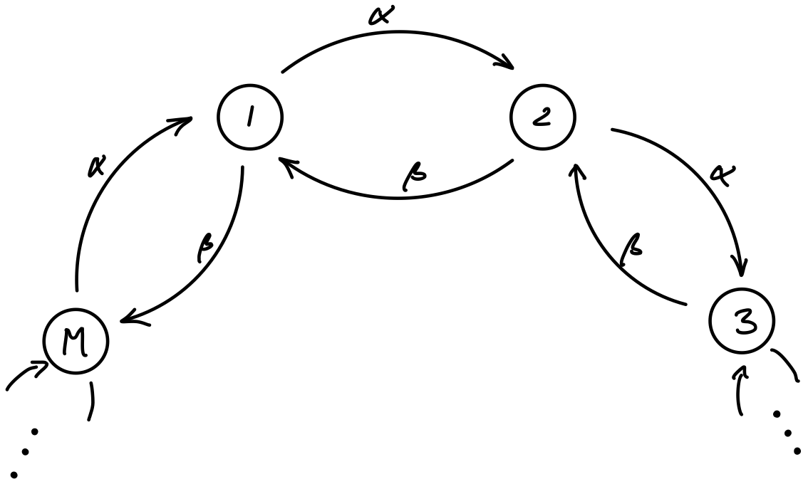
Figure S-VI.1: Cartoon of an $M$-state Markov process. Periodic states $i=1,2,\ldots,M$ are reached by transitions with rate $\alpha$ from $i-1$ and with rate $\beta$ from $i+1$.

The density and its variance at stationarity are

$$\overline{\phi}_{i}\coloneqq\lim_{t\to\infty}\mathchoice{\left\langle\phi_{i}(t)\right\rangle}{\langle\phi_{i}(t)\rangle}{\langle\phi_{i}(t)\rangle}{\langle\phi_{i}(t)\rangle}=\frac{N}{M}\ ,\quad\text{ and }\quad\lim_{t\to\infty}\mathchoice{\left\langle\phi_{i}^{2}(t)\right\rangle}{\langle\phi_{i}^{2}(t)\rangle}{\langle\phi_{i}^{2}(t)\rangle}{\langle\phi_{i}^{2}(t)\rangle}-\mathchoice{\left\langle\phi_{i}(t)\right\rangle}{\langle\phi_{i}(t)\rangle}{\langle\phi_{i}(t)\rangle}{\langle\phi_{i}(t)\rangle}^{2}=\frac{N(M-1)}{M^{2}}\,,$$ (S-VI.1)

by considering the stationary occupation of any site as a $N$-times repeated Bernoulli process with success probability $1/M$.

The entropy production of a single particle can be determined by elementary considerations Cocconi et al. (2020) to be $(\alpha-\beta)\ln(\alpha/\beta)$ so that for $N$ particles,

$$\dot{S}_{\text{int}}=N(\alpha-\beta)\ln\left(\frac{\alpha}{\beta}\right)\qquad\text{ for }\qquad M>2$$ (S-VI.2)

at stationarity, distinguishable or not. In the framework discussed in the present work, this is immediately confirmed by Eqs. (26) and Suppl. .4.

.2 Continuum particle number description

Following the approach in Nardini et al. (2017); Wittkowski et al. (2014); Tiribocchi et al. (2015), we consider the particle density field $\phi_{i}(t)$ of state $i$ as a function of time $t$ as a continuum, $\phi_{i}\in\mathds{R}$. Like Eq. (1) in Nardini et al. (2017), the density field $\phi_{i}(t)$ can be considered as being governed by a conservative Langevin equation with additive noise such as

$$\dot{\boldsymbol{\phi}}(t)=(\alpha S+\beta S^{\mathsf{T}})\boldsymbol{\phi}(t)+\sqrt{f\alpha\frac{N}{M}}S\bm{\xi}_{\alpha}(t)+\sqrt{f\beta\frac{N}{M}}S^{\mathsf{T}}\bm{\xi}_{\beta}(t)$$ (S-VI.3)

where the column vector $\boldsymbol{\phi}(t)$ has components $\phi_{i}(t)$. The matrices

$$S=\left(\begin{array}[]{rrrcrr}-1&0&0&\cdots&0&1\\ 1&-1&0&\cdots&0&0\\ 0&1&-1&\cdots&0&0\\ \vdots&\vdots&\vdots&&\vdots&\vdots\\ 0&0&0&\cdots&1&-1\end{array}\right)$$ (S-VI.4)

and its transpose $S^{\mathsf{T}}$, denoted by $\mathsf{T}$, result in a conservative movement of particles from site $i$ to $i+1$ and from $i$ to $i-1$ respectively. These matrices possess a number of very useful algebraic properties, discussed in Suppl. .3. To ease notation, we further introduce

$$\sigma\coloneqq\alpha S+\beta S^{\mathsf{T}}\ ,$$ (S-VI.5)

for the deterministic part of the Langevin Eq. (S-VI.3). Without the noise the Langevin equation is the exact master equation of a single particle. Eq. (S-VI.3) may thus be seen as an attempt to, somewhat ad hoc, express the master equation on the particle count, by adding to the single particle dynamics a noisy ”bath”.

We have introduced a fudge-factor $f$ in (S-VI.3) as a way to trace the noise amplitude through the calculation. It also provides a mechanism to adjust the noise amplitude a posteriori. The amplitude $\propto\sqrt{N/M}$ is otherwise chosen to reflect that the variance of the noise is proportional to the mean, as for a Poisson distribution. We will verify below that this choice results in the density field $\boldsymbol{\phi}$ governed by Eq. (S-VI.3) reproducing the single site variance Eq. (S-VI.1) for $f=1$. The two independent noise vectors $\bm{\xi}_{\alpha}(t)$ and $\bm{\xi}_{\beta}(t)$ have vanishing mean and correlation matrices

$$\mathchoice{\left\langle\bm{\xi}_{\alpha}(t)\bm{\xi}^{\mathsf{T}}_{\alpha}(t^{\prime})\right\rangle}{\langle\bm{\xi}_{\alpha}(t)\bm{\xi}^{\mathsf{T}}_{\alpha}(t^{\prime})\rangle}{\langle\bm{\xi}_{\alpha}(t)\bm{\xi}^{\mathsf{T}}_{\alpha}(t^{\prime})\rangle}{\langle\bm{\xi}_{\alpha}(t)\bm{\xi}^{\mathsf{T}}_{\alpha}(t^{\prime})\rangle}=\delta(t-t^{\prime})\mathbf{1} \mathchoice{\left\langle\bm{\xi}_{\beta}(t)\bm{\xi}^{\mathsf{T}}_{\beta}(t^{\prime})\right\rangle}{\langle\bm{\xi}_{\beta}(t)\bm{\xi}^{\mathsf{T}}_{\beta}(t^{\prime})\rangle}{\langle\bm{\xi}_{\beta}(t)\bm{\xi}^{\mathsf{T}}_{\beta}(t^{\prime})\rangle}{\langle\bm{\xi}_{\beta}(t)\bm{\xi}^{\mathsf{T}}_{\beta}(t^{\prime})\rangle}=\delta(t-t^{\prime})\mathbf{1}$$ and (S-VI.6)

with $\bm{\xi}_{\alpha}$ and $\bm{\xi}_{\beta}$ column vectors and $\mathbf{1}$ an $M\times M$ identity matrix. The noise vectors can, of course, be summed into a single noise term,

$$\bm{\zeta}(t;f)=\sqrt{f\alpha\frac{N}{M}}S\bm{\xi}_{\alpha}(t)+\sqrt{f\beta\frac{N}{M}}S^{\mathsf{T}}\bm{\xi}_{\beta}(t)$$ (S-VI.7)

with vanishing mean, $\mathchoice{\left\langle\bm{\zeta}(t;f)\right\rangle}{\langle\bm{\zeta}(t;f)\rangle}{\langle\bm{\zeta}(t;f)\rangle}{\langle\bm{\zeta}(t;f)\rangle}=\mathbf{0}$, and correlator

$$\mathchoice{\left\langle\bm{\zeta}(t;f)\bm{\zeta}^{\mathsf{T}}(t^{\prime};f)\right\rangle}{\langle\bm{\zeta}(t;f)\bm{\zeta}^{\mathsf{T}}(t^{\prime};f)\rangle}{\langle\bm{\zeta}(t;f)\bm{\zeta}^{\mathsf{T}}(t^{\prime};f)\rangle}{\langle\bm{\zeta}(t;f)\bm{\zeta}^{\mathsf{T}}(t^{\prime};f)\rangle}=f\frac{N}{M}(\alpha+\beta)SS^{\mathsf{T}}\delta(t-t^{\prime})\ .$$ (S-VI.8)

As shown in Suppl. .3, one eigenvalue of $S$, say $\lambda_{0}$, vanishes, which means that the corresponding $0$-mode of $\zeta$ has no variance. To write a path-density $\mathcal{P}[\bm{\zeta}(t;f)]$ for the noise in the current form, we would need to regularise this correlation matrix, as well as the deterministic part of Eq. (S-VI.3). This is straight-forwardly doable, however, somewhat messy. To avoid this distraction, we change to a basis which allows the removal of the $0$-mode from the path-densities altogether.

With the noise defined above and the deterministic part of the original Langevin Eq. (S-VI.3) effectively captured by $\sigma$, Eq. (S-VI.5), it may finally be written as

$$\dot{\boldsymbol{\phi}}(t)=\sigma\,\boldsymbol{\phi}(t)+\bm{\zeta}(t;f)\ .$$ (S-VI.9)

Eq. (S-VI.3) thus contains two approximations: Firstly, $\boldsymbol{\phi}\in\mathds{R}^{M}$ is a continuous degree of freedom that evolves without any constraints other than the conservation imposed by $S$ and $S^{\mathsf{T}}$, even though it is introduced as a local, instantaneous particle count, which requires $\phi_{i}(t)\in\mathds{N}_{0}$. Secondly, the additive noise has a (squared) amplitude proportional to the steady state $N/M$, rather than the instantaneous occupation number $\phi_{i}(t)$. There is no easy remedy for either of these two approximations, which ultimately will produce the wrong entropy production.

.3 Properties of the lattice derivative matrix $S$

The matrix $S$ as defined in Eq. (S-VI.4) plays the rôle of a spatial derivative and, unsurprisingly, has corresponding Fourier-mode eigenvectors, which we define as

$$\mathbf{e}_{\mu}=\left(\begin{array}[]{l}\mathchoice{e^{\mathring{\imath}k_{\mu}\cdot 1}}{\operatorname{exp}(\mathring{\imath}k_{\mu}\cdot 1)}{\operatorname{exp}(\mathring{\imath}k_{\mu}\cdot 1)}{\operatorname{exp}(\mathring{\imath}k_{\mu}\cdot 1)}\\ \mathchoice{e^{\mathring{\imath}k_{\mu}\cdot 2}}{\operatorname{exp}(\mathring{\imath}k_{\mu}\cdot 2)}{\operatorname{exp}(\mathring{\imath}k_{\mu}\cdot 2)}{\operatorname{exp}(\mathring{\imath}k_{\mu}\cdot 2)}\\ \mathchoice{e^{\mathring{\imath}k_{\mu}\cdot 3}}{\operatorname{exp}(\mathring{\imath}k_{\mu}\cdot 3)}{\operatorname{exp}(\mathring{\imath}k_{\mu}\cdot 3)}{\operatorname{exp}(\mathring{\imath}k_{\mu}\cdot 3)}\\ \qquad\vdots\\ \mathchoice{e^{\mathring{\imath}k_{\mu}\cdot M}}{\operatorname{exp}(\mathring{\imath}k_{\mu}\cdot M)}{\operatorname{exp}(\mathring{\imath}k_{\mu}\cdot M)}{\operatorname{exp}(\mathring{\imath}k_{\mu}\cdot M)}\end{array}\right)$$ (S-VI.10)

where the $\cdot$ is there to emphasise the multiplication in the exponent. The coefficients $k_{\mu}=2\pi\mu/M$ parameterise the $M$ distinct modes $\mu=0,1,2,\ldots,M-1$ and, in fact $\mathbf{e}_{\mu}=\mathbf{e}_{M+\mu}$. By definition, the $j$th component of $\mathbf{e}_{\mu}$ is $(\mathbf{e}_{\mu})_{j}=\mathchoice{e^{\mathring{\imath}k_{\mu}j}}{\operatorname{exp}(\mathring{\imath}k_{\mu}j)}{\operatorname{exp}(\mathring{\imath}k_{\mu}j)}{\operatorname{exp}(\mathring{\imath}k_{\mu}j)}$. Writing $S_{ij}=-\delta_{i,j}^{M}+\delta_{i-1,j}^{M}$ with

$$\delta_{i,j}^{M}=\left\{\begin{array}[]{ll}1&\text{ for }i=j\mod M\\ 0&\text{ otherwise }\end{array}\right.$$ (S-VI.11)

the eigenvalues are easily determined, $S\mathbf{e}_{\mu}=\lambda_{\mu}\mathbf{e}_{\mu}$ with

$$\lambda_{\mu}=\mathchoice{e^{-\mathring{\imath}k_{\mu}}}{\operatorname{exp}(-\mathring{\imath}k_{\mu})}{\operatorname{exp}(-\mathring{\imath}k_{\mu})}{\operatorname{exp}(-\mathring{\imath}k_{\mu})}-1$$ (S-VI.12)

and, correspondingly, $S^{\mathsf{T}}\mathbf{e}_{\mu}=\lambda^{*}_{\mu}\mathbf{e}_{\mu}$, so that the eigenvectors are orthogonal,

$$\mathbf{e}_{\mu}\cdot\mathbf{e}_{\nu}=\mathbf{e}^{\dagger}_{-\mu}\mathbf{e}_{\nu}=M\delta_{\mu+\nu,0}^{M}\ .$$ (S-VI.13)

The eigenvalue of the $0$-mode vanishes, $\lambda_{M}=\lambda_{0}=0$, and we will henceforth consider only $\mu=1,2,\ldots,M-1$.

From Eq. (S-VI.4) it follows by elementary calculation that

$$SS^{\mathsf{T}}=-\left(S+S^{\mathsf{T}}\right)=S^{\mathsf{T}}S\ ,$$ (S-VI.14)

i.e. $S$ and $S^{\mathsf{T}}$ commute. The $\mathbf{e}_{\mu}$ are also eigenvectors of $\sigma$ introduced in Eq. (S-VI.5), as $\sigma\mathbf{e}_{\mu}=p_{\mu}\mathbf{e}_{\mu}$ with

$$p_{\mu}=\alpha\lambda_{\mu}+\beta\lambda_{\mu}^{*}=-(\alpha+\beta)(1-\cos(k_{\mu}))+\mathring{\imath}(\beta-\alpha)\sin(k_{\mu})\ ,$$ (S-VI.15)

which has negative realpart for all $k_{\mu}$ as $k_{\mu}\neq 0$ for $\mu\neq 0$. The eigenvectors $\mathbf{e}_{\mu}$ can be used to re-express $\bm{\zeta}(t;f)$ and $\boldsymbol{\phi}(t)$ in terms of a more suitable basis, omitting the undesired $0$-mode, say, $\bm{\zeta}(t;f)=\frac{1}{M}\sum_{\mu=1}^{M-1}\mathbf{e}_{\mu}z_{\mu}(t;f)$, or simply

$$\bm{\zeta}(t;f)=\left(\begin{array}[]{c}\zeta_{1}(t;f)\\ \zeta_{2}(t;f)\\ \zeta_{3}(t;f)\\ \vdots\\ \zeta_{M}(t;f)\end{array}\right)=\frac{1}{M}\mathcal{E}\left(\begin{array}[]{c}z_{1}(t;f)\\ z_{2}(t;f)\\ z_{3}(t;f)\\ \vdots\\ z_{M-1}(t;f)\end{array}\right)\quad\text{ with }\quad\mathcal{E}=\left(\begin{array}[]{ccccc}\mathbf{e}_{1}&\mathbf{e}_{2}&\mathbf{e}_{3}&\ldots&\mathbf{e}_{M-1}\end{array}\right)$$ (S-VI.16)

so that the $M\times(M-1)$ matrix $\mathcal{E}$ is composed from the column vectors $\mathbf{e}_{1}$, …, $\mathbf{e}_{M-1}$, and is ”essentially unitary”, because

$$\mathcal{E}^{\dagger}=\mathcal{E}^{*\mathsf{T}}=\left(\begin{array}[]{c}\mathbf{e}^{\dagger}_{1}\\ \mathbf{e}^{\dagger}_{2}\\ \mathbf{e}^{\dagger}_{3}\\ \vdots\\ \mathbf{e}^{\dagger}_{M-1}\end{array}\right)\text{ obeys }\mathcal{E}^{\dagger}\mathcal{E}=M\mathbf{1}\ ,$$ (S-VI.17)

with $\mathbf{1}$ an $(M-1)\times(M-1)$ identity matrix, as $\mathbf{e}_{\mu}^{*}=\mathbf{e}_{-\mu}$ by construction. Of course, not being square $\mathcal{E}$ cannot be unitary and indeed $\mathcal{E}\mathcal{E}^{\dagger}$ looks rather grim, Eq. (S-VI.33). It follows that

$$\mathbf{z}(t;f)=\mathcal{E}^{\dagger}\bm{\zeta}(t;f)\ .$$ (S-VI.18)

By definition, the elements $(\mathcal{E})_{i\mu}=(\mathbf{e}_{\mu})_{i}=\mathchoice{e^{\mathring{\imath}k_{\mu}i}}{\operatorname{exp}(\mathring{\imath}k_{\mu}i)}{\operatorname{exp}(\mathring{\imath}k_{\mu}i)}{\operatorname{exp}(\mathring{\imath}k_{\mu}i)}$ depend only on the product $i\mu$ and therefore $\mathcal{E}$ is symmetric, $(\mathcal{E})_{i\mu}=(\mathcal{E})_{\mu i}$, for $1\leq i,\mu\leq M-1$. One can further show that

$$S\mathcal{E}=\mathcal{E}\Lambda\quad\text{ with }\quad\Lambda=\left(\begin{array}[]{ccccc}\lambda_{1}&&&&\mbox{\huge$0$ }\\ &\lambda_{2}\\ &&\lambda_{3}\\ &&&\ddots\\ \mbox{\huge$0$}&&&&\lambda_{M-1}\end{array}\right)\quad\text{ so that }\quad\mathcal{E}^{\dagger}S^{\mathsf{T}}=\Lambda^{*}\mathcal{E}^{\dagger}$$ (S-VI.19)

and similarly

$$S^{\mathsf{T}}\mathcal{E}=\mathcal{E}\Lambda^{*}\quad\text{ so that }\quad\mathcal{E}^{\dagger}S=\Lambda\mathcal{E}^{\dagger}\quad\text{ and }\quad\mathcal{E}^{\dagger}\sigma=\big{(}\alpha\Lambda+\beta\Lambda^{*}\big{)}\mathcal{E}^{\dagger}\ .$$ (S-VI.20)

The noise correlator of $\mathbf{z}$ is determined by Eqs. (S-VI.8) and (S-VI.18) by direct computation

$$\mathchoice{\left\langle\mathbf{z}(t;f)\mathbf{z}^{\dagger}(t^{\prime};f)\right\rangle}{\langle\mathbf{z}(t;f)\mathbf{z}^{\dagger}(t^{\prime};f)\rangle}{\langle\mathbf{z}(t;f)\mathbf{z}^{\dagger}(t^{\prime};f)\rangle}{\langle\mathbf{z}(t;f)\mathbf{z}^{\dagger}(t^{\prime};f)\rangle}=fN(\alpha+\beta)\delta(t-t^{\prime})\Lambda\Lambda^{*}$$ (S-VI.21)

using $\mathcal{E}^{\dagger}SS^{\mathsf{T}}\mathcal{E}=M\Lambda\Lambda^{*}$. As opposed to the correlator of $\zeta$, Eq. (S-VI.8), the matrix on the right can be inverted and thus be used as the basis of an Onsager-Machlup functional.

While the noise $\bm{\zeta}$ is fully determined by the noise $\mathbf{z}$, as neither has a $0$-mode, the density field $\boldsymbol{\phi}$ can have any $0$-mode, only that it does not evolve in time and therefore is not to be considered a degree of freedom. We therefore introduce the modes $a_{\mu}(t)$ of $\boldsymbol{\phi}$ with an extra parameter $\overline{\boldsymbol{\phi}}=\overline{\phi}\mathbf{e}_{0}$ that is constant in time and has identical components, so that

$$\partial_{t}\overline{\boldsymbol{\phi}}=\mathbf{0}=\sigma\overline{\boldsymbol{\phi}}\ ,$$ (S-VI.22)

and $\overline{\phi}=N/M$, Eq. (S-VI.1). Any $M$-component density field may then be written in terms of the background $\overline{\boldsymbol{\phi}}$ and an $(M-1)$-component vector $\mathbf{a}(t)$ of modes,

$$\boldsymbol{\phi}(t)=\overline{\boldsymbol{\phi}}+\frac{1}{M}\mathcal{E}\mathbf{a}(t)\ ,\quad\text{ so that }\quad\mathbf{a}(t)=\mathcal{E}^{\dagger}\boldsymbol{\phi}(t)\ .$$ (S-VI.23)

With this in place, we can write the Langevin Eq. (S-VI.9) in diagonal form, by acting from the left with $\mathcal{E}^{\dagger}$,

$$\dot{\mathbf{a}}(t)=\big{(}\alpha\Lambda+\beta\Lambda^{*}\big{)}\mathbf{a}(t)+\mathbf{z}(t;f)\ .$$ (S-VI.24)

Via Eq. (S-VI.23), Eq. (S-VI.24) provides an alternative equation of motion of the present Langevin dynamics that is more easily analysed.

.4 The Onsager-Machlup functional

The path density of the noise $\mathbf{z}$ follows from its correlator Eq. (S-VI.21) as

$$\mathcal{P}[\mathbf{z}(t;f)]\propto\operatorname{exp}\left(-\frac{1}{2fN(\alpha+\beta)}\int\mathchoice{\!\mathrm{d}t\,}{\!\mathrm{d}t\,}{\!\mathrm{d}t\,}{\!\mathrm{d}t\,}\mathbf{z}^{\dagger}(t;f)(\Lambda\Lambda^{*})^{-1}\mathbf{z}(t;f)\right)$$ (S-VI.25)

and since a path $\mathbf{z}(t)$ is uniquely determined from that of $\mathbf{a}$ and vice versa via Eq. (S-VI.24), $\mathbf{z}=\dot{\mathbf{a}}-(\alpha\Lambda+\beta\Lambda^{*})\mathbf{a}$, the Onsager-Machlup functional follows immediately, $\mathcal{P}[\mathbf{a}(t)]\propto\mathchoice{e^{\mathcal{G}[\mathbf{a}(t)]}}{\operatorname{exp}(\mathcal{G}[\mathbf{a}(t)])}{\operatorname{exp}(\mathcal{G}[\mathbf{a}(t)])}{\operatorname{exp}(\mathcal{G}[\mathbf{a}(t)])}$ with

$$\mathcal{G}[\mathbf{a}(t)]=-\frac{1}{2fN(\alpha+\beta)}\int\mathchoice{\!\mathrm{d}t\,}{\!\mathrm{d}t\,}{\!\mathrm{d}t\,}{\!\mathrm{d}t\,}\big{(}\dot{\mathbf{a}}-(\alpha\Lambda+\beta\Lambda^{*})\mathbf{a}\big{)}^{\dagger}(\Lambda\Lambda^{*})^{-1}\big{(}\dot{\mathbf{a}}-(\alpha\Lambda+\beta\Lambda^{*})\mathbf{a}\big{)}\ ,$$ (S-VI.26)

as the Jacobian is constant. By Fourier transforming the modes,

$$\mathbf{a}(\omega)=\int\mathchoice{\!\mathrm{d}t\,}{\!\mathrm{d}t\,}{\!\mathrm{d}t\,}{\!\mathrm{d}t\,}\mathchoice{e^{\mathring{\imath}\omega t}}{\operatorname{exp}(\mathring{\imath}\omega t)}{\operatorname{exp}(\mathring{\imath}\omega t)}{\operatorname{exp}(\mathring{\imath}\omega t)}\mathbf{a}(t)\quad\text{ and }\quad\mathbf{a}(t)=\int\mathchoice{\!\text{\dj}\omega\,}{\!\text{\dj}\omega\,}{\!\text{\dj}\omega\,}{\!\text{\dj}\omega\,}\mathchoice{e^{-\mathring{\imath}\omega t}}{\operatorname{exp}(-\mathring{\imath}\omega t)}{\operatorname{exp}(-\mathring{\imath}\omega t)}{\operatorname{exp}(-\mathring{\imath}\omega t)}\mathbf{a}(\omega)$$ (S-VI.27)

with $\mathchoice{\!\text{\dj}\omega\,}{\!\text{\dj}\omega\,}{\!\text{\dj}\omega\,}{\!\text{\dj}\omega\,}=\mathchoice{\!\mathrm{d}\omega\,}{\!\mathrm{d}\omega\,}{\!\mathrm{d}\omega\,}{\!\mathrm{d}\omega\,}/(2\pi)$, the Onsager-Machlup functional becomes

$$\mathcal{G}[\mathbf{a}(\omega)]=-\frac{1}{2fN(\alpha+\beta)}\int\mathchoice{\!\text{\dj}\omega\,}{\!\text{\dj}\omega\,}{\!\text{\dj}\omega\,}{\!\text{\dj}\omega\,}\mathbf{a}^{\dagger}(\omega)\big{(}\mathring{\imath}\omega\mathbf{1}+\alpha\Lambda+\beta\Lambda^{*}\big{)}^{\dagger}(\Lambda\Lambda^{*})^{-1}\big{(}\mathring{\imath}\omega\mathbf{1}+\alpha\Lambda+\beta\Lambda^{*}\big{)}\mathbf{a}(\omega)\ .$$ (S-VI.28)

Because all matrices in Eq. (S-VI.28) are diagonal the following calculations are greatly simplified. For now, we will proceed with an infinite time domain, even when the calculation of the entropy production in Section .6 will require a finite time interval to be taken to infinity systematically.

.5 Correlator of the density’s Fourier modes $\mathbf{a}(t)$

Above, it was argued that the distribution $\mathcal{P}[\mathbf{z}]$ in Eq. (S-VI.25) produces correlator Eq. (S-VI.21). Correspondingly, the distribution $\mathcal{P}[\mathbf{a}]$ with functional in Eq. (S-VI.26) produces the correlation matrix

$$\mathchoice{\left\langle\mathbf{a}(\omega)\mathbf{a}^{\dagger}(\omega^{\prime})\right\rangle}{\langle\mathbf{a}(\omega)\mathbf{a}^{\dagger}(\omega^{\prime})\rangle}{\langle\mathbf{a}(\omega)\mathbf{a}^{\dagger}(\omega^{\prime})\rangle}{\langle\mathbf{a}(\omega)\mathbf{a}^{\dagger}(\omega^{\prime})\rangle}=fN(\alpha+\beta)\left[\left(\mathring{\imath}\omega\mathbf{1}+\alpha\Lambda+\beta\Lambda^{*}\right)^{\dagger}(\Lambda\Lambda^{*})^{-1}\left(\mathring{\imath}\omega\mathbf{1}+\alpha\Lambda+\beta\Lambda^{*}\right)\right]^{-1}\delta\mkern-6.0mu\mathchar 22\relax(\omega-\omega^{\prime})\ .$$ (S-VI.29)

To invert the matrix in square brackets we use that $\Lambda$ is diagonal, so

$$\left[\left(\mathring{\imath}\omega\mathbf{1}+\alpha\Lambda+\beta\Lambda^{*}\right)^{\dagger}(\Lambda\Lambda^{*})^{-1}\left(\mathring{\imath}\omega\mathbf{1}+\alpha\Lambda+\beta\Lambda^{*}\right)\right]_{\mu\nu}=\delta_{\mu,\nu}(-\mathring{\imath}\omega+\alpha\lambda_{\mu}^{*}+\beta\lambda_{\mu})(\lambda_{\mu}^{*})^{-1}\lambda_{\mu}^{-1}(\mathring{\imath}\omega+\alpha\lambda_{\mu}+\beta\lambda^{*}_{\mu})\ .$$ (S-VI.30)

Using Eq. (S-VI.15) to write $\lambda_{\mu}$ in terms of the poles $p_{\mu}$, and $a_{\mu}^{*}(\omega)=a_{M-\mu}(-\omega)$ via Eqs. (S-VI.23) and (S-VI.27), the correlators become

$$\mathchoice{\left\langle a_{\mu}(\omega)a_{\nu}(\omega^{\prime})\right\rangle}{\langle a_{\mu}(\omega)a_{\nu}(\omega^{\prime})\rangle}{\langle a_{\mu}(\omega)a_{\nu}(\omega^{\prime})\rangle}{\langle a_{\mu}(\omega)a_{\nu}(\omega^{\prime})\rangle} =\frac{fN(\alpha+\beta)\lambda^{*}_{\mu}\lambda_{\mu}\delta^{M}_{\mu+\nu,0}\delta\mkern-6.0mu\mathchar 22\relax(\omega+\omega^{\prime})}{(-\mathring{\imath}\omega-p_{\mu})(\mathring{\imath}\omega-p_{\mu}^{*})}$$ (S-VI.31)

bound to be real, as every factor is multiplied by its complex conjugate. Both brackets in the denominator are of the form $-\mathring{\imath}\omega$ plus a number that has a strictly positive real part, as $\Re(p_{\mu})<0$, Eq. (S-VI.15).

The inverse Fourier transform of Eq. (S-VI.31) is

$$\mathchoice{\left\langle a_{\mu}(t)a_{\nu}(t^{\prime})\right\rangle}{\langle a_{\mu}(t)a_{\nu}(t^{\prime})\rangle}{\langle a_{\mu}(t)a_{\nu}(t^{\prime})\rangle}{\langle a_{\mu}(t)a_{\nu}(t^{\prime})\rangle} =\int\mathchoice{\!\text{\dj}\omega\,}{\!\text{\dj}\omega\,}{\!\text{\dj}\omega\,}{\!\text{\dj}\omega\,}\mathchoice{\!\text{\dj}\omega^{\prime}\,}{\!\text{\dj}\omega^{\prime}\,}{\!\text{\dj}\omega^{\prime}\,}{\!\text{\dj}\omega^{\prime}\,}\mathchoice{e^{-\mathring{\imath}(\omega t+\omega^{\prime}t^{\prime})}}{\operatorname{exp}(-\mathring{\imath}(\omega t+\omega^{\prime}t^{\prime}))}{\operatorname{exp}(-\mathring{\imath}(\omega t+\omega^{\prime}t^{\prime}))}{\operatorname{exp}(-\mathring{\imath}(\omega t+\omega^{\prime}t^{\prime}))}\mathchoice{\left\langle a_{\mu}(\omega)a_{\nu}(\omega^{\prime})\right\rangle}{\langle a_{\mu}(\omega)a_{\nu}(\omega^{\prime})\rangle}{\langle a_{\mu}(\omega)a_{\nu}(\omega^{\prime})\rangle}{\langle a_{\mu}(\omega)a_{\nu}(\omega^{\prime})\rangle}$$

$$=fN\delta^{M}_{\mu+\nu,0}\operatorname{exp}\left(\mathchoice{\frac{1}{2}}{(1/2)}{\frac{1}{2}}{(1/2)}(\alpha+\beta)(\lambda_{\mu}+\lambda_{\mu}^{*})|t-t^{\prime}|\right)\operatorname{exp}\left(\mathchoice{\frac{1}{2}}{(1/2)}{\frac{1}{2}}{(1/2)}(\alpha-\beta)(\lambda_{\mu}-\lambda_{\mu}^{*})(t-t^{\prime})\right)\ ,$$ (S-VI.32)

using $\lambda_{\mu}\lambda_{\mu}^{*}=-(\lambda_{\mu}+\lambda_{\mu}^{*})$ with $\Re(\lambda_{i}+\lambda_{i}^{*})=-2(1-\cos(k_{\mu}))<0$.

To validate this result, we may calculate the equal-time correlation matrix

$$\mathchoice{\left\langle(\boldsymbol{\phi}(t)-\overline{\boldsymbol{\phi}})(\boldsymbol{\phi}(t)-\overline{\boldsymbol{\phi}})^{\mathsf{T}}\right\rangle}{\langle(\boldsymbol{\phi}(t)-\overline{\boldsymbol{\phi}})(\boldsymbol{\phi}(t)-\overline{\boldsymbol{\phi}})^{\mathsf{T}}\rangle}{\langle(\boldsymbol{\phi}(t)-\overline{\boldsymbol{\phi}})(\boldsymbol{\phi}(t)-\overline{\boldsymbol{\phi}})^{\mathsf{T}}\rangle}{\langle(\boldsymbol{\phi}(t)-\overline{\boldsymbol{\phi}})(\boldsymbol{\phi}(t)-\overline{\boldsymbol{\phi}})^{\mathsf{T}}\rangle}=M^{-2}\mathcal{E}\mathchoice{\left\langle\mathbf{a}(t)\mathbf{a}^{\dagger}(t)\right\rangle}{\langle\mathbf{a}(t)\mathbf{a}^{\dagger}(t)\rangle}{\langle\mathbf{a}(t)\mathbf{a}^{\dagger}(t)\rangle}{\langle\mathbf{a}(t)\mathbf{a}^{\dagger}(t)\rangle}\mathcal{E}^{\dagger}=\frac{fN}{M^{2}}\left(\begin{array}[]{cccc}M-1&&&\mbox{\Large$-1$ }\\ &M-1\\ &&\ddots\\ \mbox{\Large$\!\!-1$ }&&&M-1\end{array}\right)$$ (S-VI.33)

via Eq. (S-VI.23) and the matrix on the far right being $\mathcal{E}\mathcal{E}^{\dagger}$, with the diagonal confirming the variance Eq. (S-VI.1) with $f=1$. Closer inspection, for example using a Doi-Peliti field theory, shows that the correlator in Eq. (S-VI.32), is exact if $f=1$. In other words, the setup Eq. (S-VI.3) captures two-point correlations exactly.

The entropy production below draws on the symmetric equal-time derivative, which we write here simply as

$$\mathchoice{\left\langle a_{\mu}(t)\dot{a}_{\nu}(t)\right\rangle}{\langle a_{\mu}(t)\dot{a}_{\nu}(t)\rangle}{\langle a_{\mu}(t)\dot{a}_{\nu}(t)\rangle}{\langle a_{\mu}(t)\dot{a}_{\nu}(t)\rangle} =\mathchoice{\frac{1}{2}}{(1/2)}{\frac{1}{2}}{(1/2)}\lim_{t^{\prime}\downarrow t}\frac{\mathrm{d}}{\mathrm{d}t^{\prime}}\mathchoice{\left\langle a_{\mu}(t)a_{\nu}(t^{\prime})\right\rangle}{\langle a_{\mu}(t)a_{\nu}(t^{\prime})\rangle}{\langle a_{\mu}(t)a_{\nu}(t^{\prime})\rangle}{\langle a_{\mu}(t)a_{\nu}(t^{\prime})\rangle}+\mathchoice{\frac{1}{2}}{(1/2)}{\frac{1}{2}}{(1/2)}\lim_{t^{\prime}\uparrow t}\frac{\mathrm{d}}{\mathrm{d}t^{\prime}}\mathchoice{\left\langle a_{\mu}(t)a_{\nu}(t^{\prime})\right\rangle}{\langle a_{\mu}(t)a_{\nu}(t^{\prime})\rangle}{\langle a_{\mu}(t)a_{\nu}(t^{\prime})\rangle}{\langle a_{\mu}(t)a_{\nu}(t^{\prime})\rangle}$$

$$=-\mathchoice{\frac{1}{2}}{(1/2)}{\frac{1}{2}}{(1/2)}fN\delta^{M}_{\mu+\nu,0}(\alpha-\beta)(\lambda_{\mu}-\lambda_{\mu}^{*})\ .$$ (S-VI.34)

.6 Entropy production

Using Seifert’s scheme Seifert (2005), the entropy production of the $M$-state Markov process with path density $\mathcal{P}([\boldsymbol{\phi}];T)$, Eq. (S-VI.26), for a path of duration $T$ is

$$\dot{S}_{\text{int}}=\lim_{T\to\infty}\frac{1}{T}\mathchoice{\left\langle\ln\left(\frac{\mathcal{P}([\boldsymbol{\phi}];T)}{\mathcal{P}([\boldsymbol{\phi}^{R}];T)}\right)\right\rangle}{\langle\ln\left(\frac{\mathcal{P}([\boldsymbol{\phi}];T)}{\mathcal{P}([\boldsymbol{\phi}^{R}];T)}\right)\rangle}{\langle\ln\left(\frac{\mathcal{P}([\boldsymbol{\phi}];T)}{\mathcal{P}([\boldsymbol{\phi}^{R}];T)}\right)\rangle}{\langle\ln\left(\frac{\mathcal{P}([\boldsymbol{\phi}];T)}{\mathcal{P}([\boldsymbol{\phi}^{R}];T)}\right)\rangle}=\lim_{T\to\infty}\frac{1}{T}\mathchoice{\left\langle\mathcal{G}([\mathbf{a}];T)-\mathcal{G}([\mathbf{a}^{R}];T)\right\rangle}{\langle\mathcal{G}([\mathbf{a}];T)-\mathcal{G}([\mathbf{a}^{R}];T)\rangle}{\langle\mathcal{G}([\mathbf{a}];T)-\mathcal{G}([\mathbf{a}^{R}];T)\rangle}{\langle\mathcal{G}([\mathbf{a}];T)-\mathcal{G}([\mathbf{a}^{R}];T)\rangle}\ ,$$ (S-VI.35)

where the constant Jacobian to transform $\boldsymbol{\phi}$ to $\mathbf{a}$ cancels in the fraction inside the logarithm and $\mathcal{G}([\mathbf{a}];T)$ is the Onsager-Machlup functional in Eq. (S-VI.26) with integration limits $0$ and $T$. In Eq. (S-VI.35), $\mathbf{a}^{R}(t)$ denotes the reverse path, $\mathbf{a}^{R}(t)=\mathbf{a}(T-t)$ so that the Onsager-Machlup functional $\mathcal{G}([\mathbf{a}^{R}];T)$ can be evaluated by replacing $\dot{\mathbf{a}^{R}}(t)$ by $-\dot{\mathbf{a}}(T-t)$. The ensemble average in Eq. (S-VI.35) needs to be taken over all allowed, accessible field configurations, but with $\boldsymbol{\phi}$ being continuous and $\overline{\boldsymbol{\phi}}$ fixed this poses no restriction. In constructing the Onsager-Machlup functional, a decision had been made implicitly or explicitly about the Itô vs. Stratonovich nature of the derivative $\dot{\mathbf{a}}$. Avoiding ambiguity, we use in the following the symmetrised version of the derivative, Eq. (S-VI.34), so that

$$\dot{S}_{\text{int}} =\lim_{T\to\infty}\frac{1}{T}\int_{0}^{T}\mathchoice{\!\mathrm{d}t\,}{\!\mathrm{d}t\,}{\!\mathrm{d}t\,}{\!\mathrm{d}t\,}\frac{1}{fN(\alpha+\beta)}\left(\mathchoice{\left\langle\dot{\mathbf{a}}(t)^{\dagger}(\Lambda\Lambda^{*})^{-1}(\alpha\Lambda+\beta\Lambda^{*})\mathbf{a}(t)\right\rangle}{\langle\dot{\mathbf{a}}(t)^{\dagger}(\Lambda\Lambda^{*})^{-1}(\alpha\Lambda+\beta\Lambda^{*})\mathbf{a}(t)\rangle}{\langle\dot{\mathbf{a}}(t)^{\dagger}(\Lambda\Lambda^{*})^{-1}(\alpha\Lambda+\beta\Lambda^{*})\mathbf{a}(t)\rangle}{\langle\dot{\mathbf{a}}(t)^{\dagger}(\Lambda\Lambda^{*})^{-1}(\alpha\Lambda+\beta\Lambda^{*})\mathbf{a}(t)\rangle}+\mathchoice{\left\langle\big{(}(\alpha\Lambda+\beta\Lambda^{*})\mathbf{a}(t)\big{)}^{\dagger}(\Lambda\Lambda^{*})^{-1}\dot{\mathbf{a}}(t)\right\rangle}{\langle\big{(}(\alpha\Lambda+\beta\Lambda^{*})\mathbf{a}(t)\big{)}^{\dagger}(\Lambda\Lambda^{*})^{-1}\dot{\mathbf{a}}(t)\rangle}{\langle\big{(}(\alpha\Lambda+\beta\Lambda^{*})\mathbf{a}(t)\big{)}^{\dagger}(\Lambda\Lambda^{*})^{-1}\dot{\mathbf{a}}(t)\rangle}{\langle\big{(}(\alpha\Lambda+\beta\Lambda^{*})\mathbf{a}(t)\big{)}^{\dagger}(\Lambda\Lambda^{*})^{-1}\dot{\mathbf{a}}(t)\rangle}\right)$$

$$=\lim_{T\to\infty}\frac{1}{T}\int_{0}^{T}\mathchoice{\!\mathrm{d}t\,}{\!\mathrm{d}t\,}{\!\mathrm{d}t\,}{\!\mathrm{d}t\,}\frac{(\alpha-\beta)^{2}}{2(\alpha+\beta)}\sum_{\mu=1}^{M-1}\left(2-\frac{\lambda_{\mu}}{\lambda_{\mu}^{*}}-\frac{\lambda_{\mu}^{*}}{\lambda_{\mu}}\right)\ .$$ (S-VI.36)

The fudge-factor $f$ has cancelled because it is the amplitude of the correlator and thus appears with its inverse in the action functional. It is obvious that this type of cancellation will occur in any bilinear action. Gone with the fudge factor is also the particle number $N$.

Otherwise, Eq. (S-VI.36) shows all the characteristics of the entropy production rate of drift-diffusion: It is quadratic in the hopping bias, $\alpha-\beta$, inversely proportional in the total hopping rate $\alpha+\beta$, which plays the rôle of a diffusion constant, and the integrand is independent of $t$, as the system is in the stationary state, so that the integral simply cancels the normalisation $1/T$. With some algebraic manipulation, $\lambda_{\mu}/\lambda^{*}_{\mu}+\lambda^{*}_{\mu}/\lambda_{\mu}=-2\cos k_{\mu}$ and $\sum_{\mu=1}^{M-1}\cos k_{\mu}=-1$ for $M\geq 2$ as $\cos k_{0}=1$, Eq. (S-VI.36) becomes

$$\dot{S}_{\text{int}}=\frac{(\alpha-\beta)^{2}}{\alpha+\beta}(M-2)\quad\text{ for }\quad M\geq 2\ .$$ (S-VI.37)

This is the final result for the entropy production on the basis of the path probability from the Langevin equation (S-VI.3) of the continuum particle number description. Taking the continuum limit $M\to\infty$ while maintaining finite drift and diffusion results in Eq. (S-VI.37) diverging.

Comparing Eq. (S-VI.37) to the exact expression Eq. (S-VI.2), immediately reveals some problems: While the logarithm might be recovered by making $\alpha-\beta$ small, the linearity in the particle number $N$ of the exact expression is replaced by a linearity in the number of states $M$ in Eq. (S-VI.37). It generally bears all the hallmarks of $M$ rather than $N$ being the number of degrees of freedom entering into this expression of the entropy production. One cannot argue that this $M$ is a proxy for the particle number $N$, as it is not multiplied by the expected particle number per site $\overline{\phi}$. As a result $\dot{S}_{\text{int}}$ of Eq. (S-VI.37) diverges as $M\to\infty$, irrespective of whether $\overline{\phi}$ is held constant or not in the limit. In short, Eq. (S-VI.37) produces the wrong result, consistent with this expression capturing the states as the degrees of freedom, rather than the particles.

It may not come as a surprise that an approximation scheme that changes the phase space from countable and discrete to uncountable and continuous shows a very different entropy production. In this light, it appears to be anything but a coarse-graining, to turn the $N$ individual degrees of freedom of positions $i\in\{1,2,\ldots,M\}$, that evolve stochastically in time, to the vastly larger phase space of a density $\phi_{i}:\{1,2,\ldots,M\}\to\mathds{R}$, similarly evolving stochastically in time.

In principle, the path probabilities and thus the entropy production in the present framework can be derived exactly on the basis of Dean’s multiplicative noise Dean (1996). However, this results in the Onsager-Machlup functional carrying an inverse of the field, which generally poses a challenge, certainly a difficult one in the presence of interaction. Even when that is overcome, the expectation in Eq. (S-VI.35) would need to be taken over the set of allowed field configurations, which now would be sums of $\delta$-functions.

This concludes the present derivation. Apparently, in this simple setup, the Langevin Eq. (S-VI.3) and the subsequent Onsager-Machlup functional Eq. (S-VI.26) capture the fluctuations correctly, but cannot be used as the starting point to construct the observable that determines the entropy production from the path probabilities, because they consider $\boldsymbol{\phi}$ as continuous degrees of freedom subject to additive noise, whereas in the original process the components of $\boldsymbol{\phi}$ are non-negative integers, $\phi_{i}\in\mathds{N}_{0}$. The relationship between Langevin equation and entropy production as exploited in Nardini et al. (2017) is in principle exact. But by assuming that the Langevin equation that approximates the dynamics can also be used to approximate the entropy production, it seems the wrong degree of freedom is subsequently considered as the one generating entropy.