The weak Galerkin finite element method for Stokes interface problems with curved interface

Abstract

In this paper, we develop a weak Galerkin (WG) finite element scheme for the Stokes interface problems with curved interfaces. The conventional numerical schemes use the straight segments to approximate the curved interfaces, and the accuracy is limited by geometric errors. Hence we directly construct the weak Galerkin finite element spaces on the curved cells to avoids geometric errors. Moreover we use non-affine transformation to convert curved cells to the reference element. Numerical integral formula in the reference element is applied to reach accuracy of weak Galerkin finite element computation. Theoretical analysis and numerical experiments show that the errors reach the optimal convergence orders under the energy norm and the $L^{2}$ norm.

1 Introduction

In this paper, we consider the Stokes interface problems. For simplicity, we describe the problems using the following model. In the model, we consider a open bounded domain $\Omega\subset\mathbb{R}^{d}\,(d=2)$ that is divided into two subdomains $\Omega_{1}$ and $\Omega_{2}$. In each subdomain $\Omega_{i},i=1,2$, the fluid flow is governed by the Stokes equations, i.e.

$$-\nabla\cdot(A_{i}\nabla{\bf u}_{i})+\nabla p_{i} = {\bf f}_{i},\,\,\qquad\text{in}\ \Omega_{i},$$ (1)

$$\nabla\cdot{\bf u}_{i} = 0,\,\,\,\qquad\text{in}\ \Omega_{i},$$ (2)

$${\bf u}_{i} = {\bf g}_{i},\qquad\text{on}\ \partial\Omega_{i}\backslash\Gamma,$$ (3)

where the viscosity coefficient $A_{i}$ is a symmetric $d\times d$ matrix-valued function in $\Omega_{i}$. Suppose that there are two positive numbers $k_{1},k_{2}\geqslant 0$ such that

$$k_{1}\alpha^{\prime}\alpha\leqslant\alpha^{\prime}A_{i}\alpha\leqslant k_{2}\alpha^{\prime}\alpha,~{}~{}~{}\forall\alpha\in\mathbb{R}^{d}.$$

For simplicity of analysis, let $A_{i}$ be the piecewise constant matrix in this paper. And $\Gamma=\partial\Omega_{1}\cap\partial\Omega_{2}$ denotes the interface of two subdomains and satisfies piecewise of $C^{2}$. The interface conditions on $\Gamma$ are described by the following equations:

$${\bf u}_{1}-{\bf u}_{2} = \mbox{\boldmath{$\phi$}},\qquad\text{on}\ \Gamma,$$ (4)

$$(A_{1}\nabla{\bf u}_{1}-p_{1}I)\mathbf{n}_{1}+(A_{2}\nabla{\bf u}_{2}-p_{2}I)\mathbf{n}_{2} = \mbox{\boldmath{$\psi$}},\qquad\text{on}\ \Gamma,$$ (5)

where $\mathbf{n}_{1}$ and $\mathbf{n}_{2}$ denote the unit outward normal vectors of $\partial\Omega_{1}$ and $\partial\Omega_{2}$ (see Figure 1) . We shall drop the subscript $i$ when velocity ${\bf u}$ and pressure $p$ are defined in the whole domain $\Omega$. The Stokes interface problems are classical fluid mechanics problems that describe the flow of viscous fluid through an interface. This type of problems has been widely applied in different fields such as groundwater resource management, petroleum engineering, biomedicine, and more [5, 8, 13, 17, 19, 23].

In practical problems, the interface is usually a complex curved surface. In two-dimensional problems, for such interfaces, we usually use straight segments to approximate curved edges. However, using high degree polynomials to approximate the solution produces geometric error. The geometric error reduces the convergence order of the error between the numerical solution and the exact solution [21, 22, 29]. Therefore, for the domain with curved edges, many numerical methods have been proposed to solving the problems on the curved domain. For example, isogeometric method [11] uses the NURBS (non-uniform rational B-splines) to approximate the whole computational domain and to construct approximation functions space. NURBS-enhanced finite element method (NEFEM) [20, 21] has the similar idea. It employs NURBS to approximate the curved domain, and uses the finite element method to solve the equations. The standard finite element method is used in the interior elements (for elements not intersecting the curved boundary), and the NURBS is used for approximation of the solution in the boundary elements (for elements intersecting the curved boundary). What’s more, there are many method to deal with curved edges, such as [1, 9, 12, 14], etc.

In this paper, we use the weak Galerkin (WG) finite element method to solve the interface problems with curved edges. The WG method was first proposed in [25] for solving second order elliptic equations. Compared with other methods, the WG method uses separate polynomial functions on each cell and adds stabilizers to the cell boundaries to ensure weak continuity of the approximative functions. Since polynomial spaces are easy to construct, the WG method can be applied to polygonal or polyhedral grids. At the same time, the WG method uses weak differential operators instead of traditional differential operators. The WG method is used to solve various problems, such as: Stokes equations [27, 30], Brinkman equations [15, 28], linear elasticity equations [24], parabolic equations[31], elliptic interface problems [16], Stokes-Darcy problems [4, 18], etc.

In this paper, we treat straight edge cells and curved cells. For the curved cells, instead of replacing curved edges with straight segments, but directly constructing the weak Galerkin finite element spaces on the curved cells. This treatment avoids geometric errors and makes the scheme easier to implement. For the calculation on the curved cells, we use non-affine transformation[32, 33] to convert curved cells to the reference element. Numerical integral formula in the reference element is applied to reach accuracy of weak Galerkin finite element computation.

The outline of this paper is as follows: in Section 2, some notations used in this paper are presented. We also give the definitions of the weak finite element spaces and weak operator, and the numerical scheme of weak Galerkin finite element method. Moreover we give the proof of the existence and uniqueness. The Section 3 is devoted to the proof of the stability of the solution of the weak Galerkin finite element scheme and some important inequalities. In Section 4 and 5, the error estimations under the energy norm and the $L^{2}$ norm are proved separately. Finally, we give some numerical examples to verify our proposed theories in Section 6.

Fig. 1: The model of Stokes-Stokes coupling flow

2 The Numerical Scheme

In this section, we first give the introduction of notations used in the paper. Next, we define the weak Galerkin finite element spaces and the corresponding weak differential operators. Finally, the weak Galerkin finite element scheme of Stokes interface problems, the proof of existence and uniqueness are given.

2.1 The notations

Assume that $\mathcal{T}_{h}$ is the polygon partition of the domain $\Omega$ containing both straight and curved cells. For $T\in\mathcal{T}_{h}$, when all edges of $T$ are straight, it is called a straight cell. The set of such straight cells is denoted by $\mathcal{T}_{h}^{S}$. When $T$ has a curved edge which intersects with the interface, it is called a curved cell. The set of the curved cells is denoted by $\mathcal{T}_{h}^{I}$. For $T\in\mathcal{T}_{h}$, let $|T|$ and $h_{T}$ be the area and the diameter of the cell $T$, respectively. Denote that $h=\max_{T\in\mathcal{T}_{h}}h_{T}$ is the mesh size. Let $\mathcal{E}_{h}$ be the set of all edges on the partition $\mathcal{T}_{h}$ and $\mathcal{E}_{h}^{0}$ be the set of all interior edges including interface edges. Denote $\mathcal{E}_{h}^{S}$ the set of all straight edges and $\mathcal{E}_{h}^{I}$ the set of all curved edges. The cell $T\in\mathcal{T}_{h}$ should satisfy following regularity conditions [27]:

(A1) Suppose that there are three positive constants $C_{1}$, $C_{2}$ and $C_{3}$ such that for every cell $T\in\mathcal{T}_{h}$ we have

$$C_{1}h_{T}^{d}\leqslant|T|,~{}~{}~{}~{}~{}C_{2}h_{e}^{d-1}\leqslant|e|,~{}~{}~{}~{}~{}|e|\leqslant C_{3}h_{T},$$ (6)

for all edges of $T$.

(A2) Suppose that there are a positive constant $\kappa$ such that for every cell $T\in\mathcal{T}_{h}$ we have

$$\kappa h_{T}\leqslant h_{e},$$ (7)

for all edges $e$ of $T$.

(A3) For every cell $T$, suppose that there exist a ball in the interior of $T$.

(A4) Assume that each $T\in\mathcal{T}_{h}$ has a circumscribed simplex $S(T)$ satisfying shape-regular conditions. And its diameter $h_{S(T)}$ is proportional to the diameter of $T$; i.e., $h_{(S(T))}\leqslant Ch_{T}$ with a constant $C$ independent of $T$. Furthermore, suppose that each circumscribed simplex $S(T)$ intersects with only a fixed and small number of such simplices for all other cells $T\in\mathcal{T}_{h}$.

2.2 Weak finite element space

We define the weak function space on the partition $\mathcal{T}_{h}$. For $T\in\mathcal{T}_{h}$, we define the weak function ${\mathbf{v}}=\{{\mathbf{v}}_{0},{\mathbf{v}}_{b}\}$ on the cell $T$, where ${\mathbf{v}}_{0}$ represents the value in the interior of $T$ and ${\mathbf{v}}_{b}$ represents the value on the boundary $\partial T$. Note that ${\mathbf{v}}_{b}$ has one unique value on the edge $e\in\mathcal{E}_{h}^{S}$ and there is two values ${\mathbf{v}}_{1b}$ and ${\mathbf{v}}_{2b}$ on the edge $e\in\mathcal{E}_{h}^{I}$. And there is no relationship between the value of ${\mathbf{v}}_{0}$ and ${\mathbf{v}}_{b}$. Next, we give some definitions of some projection operators. Let $Q_{0}$ be the $L^{2}$ projection operator from $[L^{2}(T)]^{d}$ onto $[P_{k}(T)]^{d}$, $T\in\mathcal{T}_{h}$. For each edge $e\in\mathcal{E}_{h}$, $Q_{b}$ is defined as the $L^{2}$ projection operator from $[L^{2}(e)]^{d}$ onto $[P_{k-1}(e)]^{d}$ when $e\in\mathcal{E}_{h}^{S}$, and from $[L^{2}(e)]^{d}$ onto $[P_{k}(e)]^{d}$ when $e\in\mathcal{E}_{h}^{I}$. Finally, we give the weak Galerkin finite element spaces with respect to the velocity ${\bf u}$ and the pressure $p$. For a given integer $k\geqslant 1$,

$$V_{h}= \{{\mathbf{v}}=\{{\mathbf{v}}_{0},{\mathbf{v}}_{b}\}:{\mathbf{v}}_{0}|_{T}\in[P_{k}(T)]^{d},\,T\in\mathcal{T}_{h},$$

$${\mathbf{v}}_{b}|_{e}\in[P_{k-1}(e)]^{d},e\in\mathcal{E}_{h}^{S},{\mathbf{v}}_{b}|_{e}\in[P_{k}(e)]^{d},{\mathbf{v}}_{1b}-{\mathbf{v}}_{2b}=Q_{b}\mbox{\boldmath{$\phi$}},e\in\mathcal{E}_{h}^{I}\},$$

$$V_{h}^{0}= \{{\mathbf{v}}=\{{\mathbf{v}}_{0},{\mathbf{v}}_{b}\}\in V_{h},{\mathbf{v}}_{b}=\mathbf{0}~{}on~{}\partial\Omega,{\mathbf{v}}_{1b}-{\mathbf{v}}_{2b}=\mathbf{0},e\in\mathcal{E}_{h}^{I}\},$$

$$W_{h}= \{q:q\in L_{0}^{2}(\Omega),q|_{T}\in P_{k-1}(T),\,T\in\mathcal{T}_{h}\}.$$

Firstly, we introduce some weak differential operators used in this paper.

Definition 1.

For each ${\mathbf{v}}\in V_{h}$, its discrete weak gradient is denoted by $\nabla_{w}{\mathbf{v}}\in[P_{k-1}(T)]^{d\times d}$ and satisfies the following equation:

$$(\nabla_{w}{\mathbf{v}},q)_{T}=-({\mathbf{v}}_{0},\nabla\cdot q)_{T}+\langle{\mathbf{v}}_{b},q\cdot{\bf n}\rangle_{\partial T},~{}\forall~{}q\in[P_{k-1}(T)]^{d\times d},$$ (8)

where ${\bf n}$ is the unit outward normal vector on $\partial T$.

Similarly, we give the definition of discrete weak divergence operator.

Definition 2.

For each ${\mathbf{v}}\in V_{h}$, its discrete weak divergence is denoted by $\nabla_{w}\cdot{\mathbf{v}}\in P_{k-1}(T)$ and satisfies the following equation:

$$(\nabla_{w}\cdot{\mathbf{v}},\tau)_{T}=-({\mathbf{v}}_{0},\nabla\tau)_{T}+\langle{\mathbf{v}}_{b},\tau{\bf n}\rangle_{\partial T},~{}\forall~{}\tau\in P_{k-1}(T),$$ (9)

2.3 The numerical scheme

Next, we introduce some bilinear forms as follows: for all ${\mathbf{v}}$, ${\bf w}\in V_{h}$,

$$s({\mathbf{v}},{\bf w}) = \sum_{T\in\mathcal{T}_{h}}h_{T}^{-1}\left(\langle Q_{b}{\mathbf{v}}_{0}-{\mathbf{v}}_{b},Q_{b}{\bf w}_{0}-{\bf w}_{b}\rangle_{\partial T\setminus(\partial T\cap\Gamma)}+\langle{\mathbf{v}}_{0}-{\mathbf{v}}_{b},{\bf w}_{0}-{\bf w}_{b}\rangle_{\partial T\cap\Gamma}\right)$$

$$a({\mathbf{v}},{\bf w}) = \sum_{T\in\mathcal{T}_{h}}(A\nabla_{w}{\mathbf{v}},\nabla_{w}{\bf w})_{T},$$

$$a_{s}({\mathbf{v}},{\bf w}) = a({\mathbf{v}},{\bf w})+s({\mathbf{v}},{\bf w}),$$

$$b({\mathbf{v}},p) = -\sum_{T\in\mathcal{T}_{h}}(\nabla_{w}\cdot{\mathbf{v}},p)_{T}.$$

Weak Galerkin Algorithm 1.

For the Stokes interface problems (1)-(5), the weak Galerkin finite element method is seeking $\mathbf{u}_{h}\in V_{h}$, and $p_{h}\in W_{h}$ such that ${\bf u}_{b}=Q_{b}{\bf g}~{}\text{on}\ \partial\Omega$ and

$$a_{s}({\bf u}_{h},{\mathbf{v}}_{h})+b({\mathbf{v}}_{h},p_{h}) = ({\bf f},{\mathbf{v}}_{0})+\langle\mbox{\boldmath{$\psi$}},{\mathbf{v}}_{b}\rangle_{\Gamma},~{}~{}\forall~{}{\mathbf{v}}_{h}\in V_{h}^{0},$$ (10)

$$b({\bf u}_{h},q_{h}) = 0,~{}~{}~{}~{}~{}~{}~{}~{}~{}~{}~{}~{}~{}~{}~{}~{}~{}~{}~{}~{}~{}~{}\forall~{}q_{h}\in W_{h}.$$ (11)

We now define a semi-norm in the weak Galerkin finite element space $V_{h}$ as follows:

$${|||}{\mathbf{v}}{|||}^{2}=a_{s}({\mathbf{v}},{\mathbf{v}}).$$ (12)

Then we have the following properties.

Lemma 3.

${|||}\cdot{|||}$ provides a norm in $V_{h}^{0}$.

Proof.

It’s easy to see that the triangle inequality and linear property for ${|||}\cdot{|||}$. Next, assume that ${|||}{\mathbf{v}}{|||}=0$ for some ${\mathbf{v}}\in V_{h}^{0}$, then it follows that

$$0=a_{s}({\mathbf{v}},{\mathbf{v}})=\sum_{T\in\mathcal{T}_{h}}(A\nabla_{w}{\mathbf{v}},\nabla_{w}{\mathbf{v}})_{T}+\sum_{T\in\mathcal{T}_{h}}h_{T}^{-1}\left(\langle Q_{b}{\mathbf{v}}_{0}-{\mathbf{v}}_{b},Q_{b}{\mathbf{v}}_{0}-{\mathbf{v}}_{b}\rangle_{\partial T\backslash\Gamma}+\langle{\mathbf{v}}_{0}-{\mathbf{v}}_{b},{\mathbf{v}}_{0}-{\mathbf{v}}_{b}\rangle_{\partial T\cap\Gamma}\right).$$

The above equation implies the following conclusions:

1. $\nabla_{w}{\mathbf{v}}=0$ on all $T\in\mathcal{T}_{h}$;
   

2. $Q_{b}{\mathbf{v}}_{0}={\mathbf{v}}_{b}$ for $e\in\mathcal{E}_{h}^{S}$;
   

3. ${\mathbf{v}}_{0}={\mathbf{v}}_{b}$ for $e\in\mathcal{E}_{h}^{I}$.

Therefore, for any $q\in[P_{k-1}(T)]^{d\times d}$, we have the following identities.

(1)For $T\in\mathcal{T}_{h}^{S}$,

$$0= (\nabla_{w}{\mathbf{v}},q)_{T}$$

$$= -({\mathbf{v}}_{0},\nabla\cdot q)_{T}+\langle{\mathbf{v}}_{b},q{\bf n}\rangle_{\partial T}$$

$$= (\nabla{\mathbf{v}}_{0},q)_{T}-\langle{\mathbf{v}}_{0},q{\bf n}\rangle_{\partial T}+\langle{\mathbf{v}}_{b},q{\bf n}\rangle_{\partial T}$$

$$= (\nabla{\mathbf{v}}_{0},q)_{T}-\langle Q_{b}{\mathbf{v}}_{0}-{\mathbf{v}}_{b},q{\bf n}\rangle_{\partial T}$$

$$= (\nabla{\mathbf{v}}_{0},q)_{T}.$$

(2)For $T\in\mathcal{T}_{h}^{I}$,

$$0= (\nabla_{w}{\mathbf{v}},q)_{T}$$

$$= -({\mathbf{v}}_{0},\nabla\cdot q)_{T}+\langle{\mathbf{v}}_{b},q{\bf n}\rangle_{\partial T}$$

$$= (\nabla{\mathbf{v}}_{0},q)_{T}-\langle{\mathbf{v}}_{0},q{\bf n}\rangle_{\partial T}+\langle{\mathbf{v}}_{b},q{\bf n}\rangle_{\partial T}$$

$$= (\nabla{\mathbf{v}}_{0},q)_{T}-\langle Q_{b}{\mathbf{v}}_{0}-{\mathbf{v}}_{b},q{\bf n}\rangle_{\partial T\backslash\Gamma}-\langle{\mathbf{v}}_{0}-{\mathbf{v}}_{b},q{\bf n}\rangle_{\partial T\cap\Gamma}$$

$$= (\nabla{\mathbf{v}}_{0},q)_{T}$$

In the above equations letting $q=\nabla{\mathbf{v}}_{0}$ derives $\nabla{\mathbf{v}}_{0}=0$ on each cell $T\in\mathcal{T}_{h}$. It follows that ${\mathbf{v}}_{0}$ is constant on each cell $T\in\mathcal{T}_{h}$. Due to ${\mathbf{v}}_{0}=Q_{b}{\mathbf{v}}_{0}={\mathbf{v}}_{b}$ when $e\in\mathcal{E}_{h}$, we have ${\mathbf{v}}_{0}={\mathbf{v}}_{b}=C$. This together with the fact that ${\mathbf{v}}_{b}=0$ on $\partial\Omega$ implies that ${\mathbf{v}}_{0}=0$ and ${\mathbf{v}}_{b}=0$. ∎

Lemma 4.

For any ${\mathbf{v}},{\bf w}\in V_{h}^{0}$,

$$|a({\mathbf{v}},{\bf w})| \leqslant {|||}{\mathbf{v}}{|||}\cdot{|||}{\bf w}{|||},$$ (13)

$$a({\mathbf{v}},{\mathbf{v}}) = {|||}{\mathbf{v}}{|||}^{2}.$$ (14)

Lemma 5.

The weak Galerkin finite element schemes (10)-(11) have one and only one solution.

Proof.

Since the number of equations is the same as the number of unknowns, existence and uniqueness are equivalent. Let $\{{\bf u}_{h},p_{h}\}$ and $\{{\bf u}_{h}^{\prime},p_{h}^{\prime}\}$ be the solutions of the schemes (10)-(11) respectively. So the following equations hold true:

$$a_{s}({\bf u}_{h},{\mathbf{v}}_{h})+b({\mathbf{v}}_{h},p_{h}) = ({\bf f},{\mathbf{v}}_{0})+\langle\mbox{\boldmath{$\psi$}},{\mathbf{v}}_{b}\rangle_{\Gamma},$$ (15)

$$b({\bf u}_{h},q_{h}) = 0,$$ (16)

$$a_{s}({\bf u}_{h}^{\prime},{\mathbf{v}}_{h})+b({\mathbf{v}}_{h},p_{h}^{\prime}) = ({\bf f},{\mathbf{v}}_{0})+\langle\mbox{\boldmath{$\psi$}},{\mathbf{v}}_{b}\rangle_{\Gamma},$$ (17)

$$b({\bf u}_{h}^{\prime},q_{h}) = 0.$$ (18)

Subtracting Eq.(17) from Eq.(15) and subtracting Eq.(18) from Eq.(16) derive that

$$a_{s}({\bf u}_{h}-{\bf u}_{h}^{\prime},{\mathbf{v}}_{h})+b({\mathbf{v}}_{h},p_{h}-p_{h}^{\prime})=0,$$ (19)

$$b({\bf u}_{h}-{\bf u}_{h}^{\prime},q_{h})=0.$$ (20)

Letting ${\mathbf{v}}_{h}={\bf u}_{h}-{\bf u}_{h}^{\prime}\in V_{h}^{0}$ in Eq. (19) and $q_{h}=p_{h}-p_{h}^{\prime}\in W_{h}$ in Eq.(20) leads to

$$a_{s}({\bf u}_{h}-{\bf u}_{h}^{\prime},{\bf u}_{h}-{\bf u}_{h}^{\prime})+b({\bf u}_{h}-{\bf u}_{h}^{\prime},p_{h}-p_{h}^{\prime})=0,$$ (21)

$$b({\bf u}_{h}-{\bf u}_{h}^{\prime},p_{h}-p_{h}^{\prime})=0.$$ (22)

Since ${|||}\cdot{|||}$ is a norm in $V_{h}^{0}$, we obtain ${\bf u}_{h}={\bf u}_{h}^{\prime}$ and $b({\mathbf{v}}_{h},p_{h}-p_{h}^{\prime})=0$. Then we take ${\mathbf{v}}_{h}=\{\nabla(p_{h}-p_{h}^{\prime}),0\}$ to obtain the result $0=\sum_{T\in\mathcal{T}_{h}}\|\nabla(p_{h}-p_{h}^{\prime})\|_{T}^{2}$. It follows that $\nabla(p_{h}-p_{h}^{\prime})=0$, $\forall~{}T\in\mathcal{T}_{h}$ and $p_{h}-p_{h}^{\prime}$ is constant $on~{}T\in\mathcal{T}_{h}$.

Next, taking ${\mathbf{v}}_{0}=0$ on $T\in\mathcal{T}_{h}$, ${\mathbf{v}}_{b}={[\![}p_{h}-p_{h}^{\prime}{]\!]}{\bf n}_{e}$, $e\in\mathcal{E}_{h}^{S}$ and ${\mathbf{v}}_{b}=0$ on $e\in\mathcal{E}_{h}^{I}$ in Eq.(19) leads to the fact that $\sum_{e\in\mathcal{E}_{h}^{S}}\|{[\![}p_{h}-p_{h}^{\prime}{]\!]}{\bf n}_{e}\|_{e}^{2}=0$. Moreover, when $e\in\mathcal{E}_{h}^{I}$, denote the other two edges of the same cell by $e_{1}$ and $e_{2}$ and their unit outward normal vectors by ${\bf n}_{e_{1}}$ and ${\bf n}_{e_{2}}$. We take ${\mathbf{v}}_{0}=0$ on $T\in\mathcal{T}_{h}$, ${\mathbf{v}}_{b}=0$ on $e\in\mathcal{E}_{h}^{S}$ and ${\mathbf{v}}_{b}={[\![}p_{h}-p_{h}^{\prime}{]\!]}({\bf n}_{e_{1}}+{\bf n}_{e_{2}})$ on $e\in\mathcal{E}_{h}^{I}$ to derive that $0={[\![}p_{h}-p_{h}^{\prime}{]\!]}_{e}^{2}\langle{\bf n}_{e_{1}}+{\bf n}_{e_{2}},{\bf n}_{e}\rangle_{e}$. Since $\langle({\bf n}_{e_{1}}+{\bf n}_{e_{2}}),{\bf n}_{e}\rangle_{e}<0$, we get ${[\![}p_{h}-p_{h}^{\prime}{]\!]}_{e}=0$. Noting that $p_{h}\in L_{0}^{2}(\Omega)$, we have $p_{h}-p_{h}^{\prime}=0$. Therefore we have $p_{h}-p_{h}^{\prime}=C~{}on~{}\Omega$. The proof of uniqueness is completed. ∎

3 Stability

For $T\in\mathcal{T}_{h}$, let $Q_{h}=\{Q_{0},~{}Q_{b}\}$ be the $L^{2}$ projection operator onto $V_{h}$. $\mathcal{Q}_{h}$ and $\mathbb{Q}_{h}$ are defined as the $L^{2}$ projection operators onto $P_{k-1}(T)$ and $[P_{k-1}(T)]^{d\times d}$, respectively.

Lemma 6.

On each cell $T\in\mathcal{T}_{h}$, for the discrete weak gradient operator, we have the following properties.

(1)For $T\in\mathcal{T}_{h}^{S}$, we have

$$(\nabla_{w}(Q_{h}{\bf u}),\tau)_{T}=(\mathbb{Q}_{h}(\nabla{\bf u}),\tau)_{T},~{}\forall~{}\tau\in[P_{k-1}(T)]^{d\times d},$$ (23)

(2)For $T\in\mathcal{T}_{h}^{I}$, we have

$$(\nabla_{w}(Q_{h}{\bf u}),\tau)_{T}=(\mathbb{Q}_{h}(\nabla{\bf u}),\tau)_{T}+\langle Q_{b}{\bf u}-{\bf u},\tau{\bf n}\rangle_{\partial T\cap\Gamma},~{}~{}\forall~{}\tau\in[P_{k-1}(T)]^{d\times d}.$$ (24)

Proof.

According to Eq.(1), definitions of $Q_{0}$, $Q_{b}$ and $\mathbb{Q}_{h}$, the integration by parts and $\tau\in[P_{k-1}(T)]^{d\times d}$, we have for $T$ $\in\mathcal{T}_{h}^{S}$,

$$(\nabla_{w}(Q_{h}{\bf u}),\tau)_{T}= -(Q_{0}{\bf u},\nabla\cdot\tau)_{T}+\langle Q_{b}{\bf u},\tau\cdot{\bf n}\rangle_{\partial T}$$

$$= -({\bf u},\nabla\cdot\tau)_{T}+\langle{\bf u},\tau\cdot{\bf n}\rangle_{\partial T}$$

$$= (\nabla{\bf u},\tau)_{T}$$

$$= (\mathbb{Q}_{h}(\nabla{\bf u}),\tau)_{T}.$$

Similarly, we have for $T$ $\in\mathcal{T}_{h}^{I}$,

$$(\nabla_{w}(Q_{h}{\bf u}),\tau)_{T}= -(Q_{0}{\bf u},\nabla\cdot\tau)_{T}+\langle Q_{b}{\bf u},\tau\cdot{\bf n}\rangle_{\partial T}$$

$$= -({\bf u},\nabla\cdot\tau)_{T}+\langle{\bf u},\tau\cdot{\bf n}\rangle_{\partial T}+\langle Q_{b}{\bf u}-{\bf u},\tau\cdot{\bf n}\rangle_{\partial T\cap\Gamma}$$

$$= (\nabla{\bf u},\tau)_{T}+\langle Q_{b}{\bf u}-{\bf u},\tau\cdot{\bf n}\rangle_{\partial T\cap\Gamma}$$

$$= (\mathbb{Q}_{h}(\nabla{\bf u}),\tau)_{T}+\langle Q_{b}{\bf u}-{\bf u},\tau\cdot{\bf n}\rangle_{\partial T\cap\Gamma}.$$

The proof of the Lemma 6 is completed. ∎

Lemma 7.

On each cell $T\in\mathcal{T}_{h}$, for the weak divergence operator, we have the following properties:

(1)For $T\in\mathcal{T}_{h}^{S}$, we obtain

$$(\nabla_{w}\cdot(Q_{h}{\bf u}),\varphi)_{T}=(\mathcal{Q}_{h}(\nabla\cdot{\bf u}),\varphi)_{T},~{}\forall~{}\varphi\in P_{k-1}(T),$$ (25)

(2)For $T\in\mathcal{T}_{h}^{I}$, we obtain

$$(\nabla_{w}\cdot(Q_{h}{\bf u}),\varphi)_{T}=(\mathcal{Q}_{h}(\nabla\cdot{\bf u}),\varphi)_{T}+\langle Q_{b}{\bf u}-{\bf u},\varphi{\bf n}\rangle_{\partial T\cap\Gamma},~{}~{}\forall~{}\varphi\in P_{k-1}(T).$$ (26)

Proof.

For $T\in\mathcal{T}_{h}^{S}$, according to the Eq.(2), definitions of $Q_{0}$, $Q_{b}$ and $\mathcal{Q}_{h}$, the integration by parts and $\varphi\in P_{k-1}(T)$, we have

$$(\nabla_{w}\cdot(Q_{h}{\bf u}),\varphi)_{T}= -(Q_{0}{\bf u},\nabla\varphi)_{T}+\langle Q_{b}{\bf u},\varphi{\bf n}\rangle_{\partial T}$$

$$= -({\bf u},\nabla\varphi)_{T}+\langle{\bf u},\varphi{\bf n}\rangle_{\partial T}$$

$$= (\nabla\cdot{\bf u},\varphi)_{T}$$

$$= (\mathcal{Q}_{h}(\nabla\cdot{\bf u}),\varphi)_{T}.$$

Next, for $T\in\mathcal{T}_{h}^{I}$, using Eq.(2),

$$(\nabla_{w}\cdot(Q_{h}{\bf u}),\varphi)_{T}= -(Q_{0}{\bf u},\nabla\varphi)_{T}+\langle Q_{b}{\bf u},\varphi{\bf n}\rangle_{\partial T}$$

$$= -({\bf u},\nabla\varphi)_{T}+\langle{\bf u},\varphi{\bf n}\rangle_{\partial T}+\langle Q_{b}{\bf u}-{\bf u},\varphi{\bf n}\rangle_{\partial T\cap\Gamma}$$

$$= (\nabla\cdot{\bf u},\varphi)_{T}+\langle Q_{b}{\bf u}-{\bf u},\varphi{\bf n}\rangle_{\partial T\cap\Gamma}$$

$$= (\mathcal{Q}_{h}(\nabla\cdot{\bf u}),\varphi)_{T}+\langle Q_{b}{\bf u}-{\bf u},\varphi{\bf n}\rangle_{\partial T\cap\Gamma}.$$

The proof of the above lemma is completed. ∎

Now, we give some important inequalities for the proof. The trace inequality and the inverse inequality are essential technique tools for the analysis. For the straight triangular cells, these inequalities have been proved in [26]. Next we shall extend two inequalities to the curved triangular cells.

Lemma 8.

(Inverse inequality) For all $T\in\mathcal{T}_{h}^{I}$, $\varphi$ is the piecewise polynomial on $T$, then we have

$$\|\nabla\varphi\|_{T}\leqslant Ch_{T}^{-1}\|\varphi\|_{T}.$$ (27)

Proof.

For any $T\in\mathcal{T}_{h}^{I}$, assuming that $S(T)$ is the circumscribed simplex satisfying the shape regularity conditions. According to the standard inverse inequality on $S(T)$, we have

$$\|\nabla\varphi\|_{T}\leqslant\|\nabla\varphi\|_{S(T)}\leqslant Ch_{S(T)}^{-1}\|\varphi\|_{S(T)}.$$

Next let $S$ be a ball inside of $T$ with a diameter proportional to $h_{T}$. Then by the domain inverse inequality we get

$$\|\varphi\|_{S(T)}\leqslant\|\varphi\|_{S}\leqslant\|\varphi\|_{T}.$$

Substituting into the above inequality leads to

$$\|\nabla\varphi\|_{T}\leqslant Ch_{T}^{-1}\|\varphi\|_{T}.$$

The proof of the inverse inequality on the curved cells is completed. ∎

Lemma 9.

(Trace inequality) For any $T\in\mathcal{T}_{h}^{I}$, $\varphi\in H^{1}(T)$, we have

$$\|\varphi\|_{e}^{2}\leqslant C\left(h_{T}^{-1}\|\varphi\|_{T}^{2}+h_{T}\|\nabla\varphi\|_{T}^{2}\right),~{}~{}e\subset\partial T.$$ (28)

Proof.

For simplify, let’s consider triangular cells. Similarly, the trace inequality holds for polygons. When $T\in\mathcal{T}_{h}^{I}$, we assume that the transformation between $T$ and the reference element $\hat{T}$ is as follows

$$\left\{\begin{array}[]{rl}x=\tilde{x}(\xi,\eta),&(\xi,\eta)\in\hat{T}\\ y=\tilde{y}(\xi,\eta),&(\xi,\eta)\in\hat{T}\end{array}\right..$$

and denote that $\tilde{\varphi}(\xi,\eta)=\varphi(\tilde{x}(\xi,\eta),\tilde{y}(\xi,\eta))$ and $\tilde{J}$ is the Jacobian of the above mapping. Assuming that the edge $e$ has the parametric representation $x=x(t)$, $y=y(t)$, $0\leqslant t\leqslant 1$. According to regularity conditions and Theorem 1 in [32], every term in Eq.(28) has the following estimate.

$$\|\varphi\|_{e}^{2}=\int_{e}\varphi^{2}(x,y)ds=\int_{0}^{1}\varphi^{2}(x(t),y(t))|e|dt=\int_{0}^{1}\tilde{\varphi}^{2}(\xi(t),\eta(t))|e|dt\leqslant Ch_{T}\int_{0}^{1}\tilde{\varphi}^{2}|\hat{e}|dt,$$

and

$$\begin{split}\|\varphi\|_{T}^{2}=&\int_{T}\varphi(x,y)^{2}dT\\ =&\int_{\hat{T}}\tilde{\varphi}^{2}(\xi,\eta)|\tilde{J}|d\hat{T}\\ \geqslant&Ch_{T}^{2}\int_{\hat{T}}\tilde{\varphi}^{2}(\xi,\eta)d\hat{T}\\ \geqslant&Ch_{T}^{2}{h^{-1}_{\hat{T}}}\int_{\hat{T}}\tilde{\varphi}^{2}(\xi,\eta)d\hat{T},\end{split}$$

and

$$\begin{split}\|\nabla\varphi\|_{T}^{2}=&\int_{T}\left(\frac{\partial\varphi}{\partial x}(x,y)\right)^{2}+\left(\frac{\partial\varphi}{\partial y}(x,y)\right)^{2}dT\\ =&\int_{\hat{T}}\left(\frac{\partial\varphi}{\partial x}(\tilde{x}(\xi,\eta),\tilde{y}(\xi,\eta))\right)^{2}+\left(\frac{\partial\varphi}{\partial y}(\tilde{x}(\xi,\eta),\tilde{y}(\xi,\eta))\right)^{2}|\tilde{J}|d\hat{T}\\ \geqslant&\int_{\hat{T}}\left(\frac{\partial\varphi}{\partial x}(\tilde{x}(\xi,\eta),\tilde{y}(\xi,\eta))\right)^{2}+\left(\frac{\partial\varphi}{\partial y}(\tilde{x}(\xi,\eta),\tilde{y}(\xi,\eta))\right)^{2}h_{T}^{2}d\hat{T}\\ \geqslant&C\int_{\hat{T}}\left(\frac{\partial\varphi}{\partial x}(\tilde{x}(\xi,\eta),\tilde{y}(\xi,\eta))+\frac{\partial\varphi}{\partial y}(\tilde{x}(\xi,\eta),\tilde{y}(\xi,\eta))\right)\Big{[}(\frac{\partial\tilde{x}}{\partial\xi}+\frac{\partial\tilde{y}}{\partial\xi})^{2}+(\frac{\partial\tilde{x}}{\partial\eta}+\frac{\partial\tilde{y}}{\partial\eta})^{2}\Big{]}d\hat{T}\\ \geqslant&C\int_{\hat{T}}\left(\frac{\partial\varphi}{\partial x}\frac{\partial\tilde{x}}{\partial\xi}+\frac{\partial\varphi}{\partial y}\frac{\partial\tilde{y}}{\partial\xi}\right)^{2}+\left(\frac{\partial\varphi}{\partial x}\frac{\partial\tilde{x}}{\partial\eta}+\frac{\partial\varphi}{\partial y}\frac{\partial\tilde{y}}{\partial\eta}\right)^{2}d\hat{T}\\ =&\int_{\hat{T}}\left(\frac{\partial\tilde{\varphi}}{\partial\xi}\right)^{2}+\left(\frac{\partial\tilde{\varphi}}{\partial\eta}\right)^{2}d\hat{T}\\ \geqslant&Ch_{\hat{T}}\|\nabla\tilde{\varphi}\|_{\hat{T}}.\end{split}$$

Therefore, according to the trace inequality on the reference elements, we have

$$\begin{split}\|\varphi\|_{e}^{2}\leqslant&Ch_{T}\|\tilde{\varphi}\|_{\hat{e}}^{2}\\ \leqslant&Ch_{T}h_{\hat{T}}^{-1}\|\tilde{\varphi}\|_{\hat{T}}^{2}+Ch_{T}h_{\hat{T}}\|\nabla\tilde{\varphi}\|_{\hat{T}}^{2}\\ \leqslant&Ch_{T}^{-1}\|\varphi\|_{T}^{2}+Ch_{T}\|\nabla\varphi\|_{T}^{2}.\end{split}$$

The proof of the trace inequality is completed. ∎

Lemma 10.

[27] Let $\mathcal{T}_{h}$ be finite element partition of $\Omega$ satisfying the shape regularity conditions and ${\bf w}\in[H^{r+1}(\Omega)]^{d}$ and $\rho\in H^{r}(\Omega)$ with $1\leqslant r\leqslant k$. Then, for $0\leqslant s\leqslant 1$ we have

$$\sum_{T\in\mathcal{T}_{h}}h_{T}^{2s}\|{\bf w}-Q_{0}{\bf w}\|_{T,s}^{2} \leqslant Ch^{2(r+1)}\|{\bf w}\|_{r+1}^{2},$$ (30)

$$\sum_{T\in\mathcal{T}_{h}}h_{T}^{2s}\|\nabla{\bf w}-\mathbb{Q}_{h}(\nabla{\bf w})\|_{T,s}^{2} \leqslant Ch^{2r}\|{\bf w}\|_{r+1}^{2},$$ (31)

$$\sum_{T\in\mathcal{T}_{h}}h_{T}^{2s}\|\rho-\mathcal{Q}_{h}\rho\|_{T,s}^{2} \leqslant Ch^{2r}\|\rho\|_{r}^{2}.$$ (32)

Here C denotes a generic constant independent of the mesh size h and the functions in the estimates.

Proof.

For $T\in\mathcal{T}_{h}$, we assume that $S(T)$ is the circumscribed simplex satisfying the shape regularity conditions. And let $u$ smoothly extend onto $S(T)$. Denote by $\tilde{Q}_{0}$ the $L^{2}$ projection operator onto $[P_{k}(S(T))]^{2}$. Then we have

$$\sum_{T\in\mathcal{T}_{h}}\|u-Q_{0}u\|_{T}^{2}\leqslant C\sum_{T\in\mathcal{T}_{h}}\|u-\tilde{Q}_{0}u\|_{T}^{2}\leqslant C\sum_{T\in\mathcal{T}_{h}}\|u-\tilde{Q}_{0}u\|_{S(T)}^{2}\leqslant Ch_{S(T)}^{2(r+1)}\|u\|_{r+1,S(T)}^{2}\leqslant Ch_{T}^{2(r+1)}\|u\|_{r+1,S(T)}^{2}.$$

From the regularity conditions, the number of overlaps of circumscribed simplex sets is fixed, then we derive

$$\sum_{T\in\mathcal{T}_{h}}\|u-Q_{0}u\|_{T}^{2}\leqslant Ch^{2(r+1)}\|u\|_{r+1}^{2}.$$

Similarly, we can get

$$\sum_{T\in\mathcal{T}_{h}}h_{T}^{2s}\|\nabla(u-Q_{0}u)\|_{T,s}^{2}\leqslant Ch^{2(r+1)}\|u\|_{r+1}^{2}.$$

Therefore, the proof of Eq.(30) is completed. The proof of the Eqs.(31)-(32) is quite similar to the Eq.(30) and so is omitted. ∎

Next we give the stability analysis of the Stokes interface problems.

Lemma 11.

(Inf-sup condition) There exist two positive constants $C_{1}$ and $C_{2}$ such that

$$\sup_{{\mathbf{v}}\in V_{h}^{0}}\frac{b({\mathbf{v}},\rho)}{{|||}{\mathbf{v}}{|||}}\geqslant C_{1}\|\rho\|-C_{2}h|\rho|_{1},$$ (33)

for all $\rho\in W_{h}$, where $C_{1}$ and $C_{2}$ are independent of the mesh size $h$.

Proof.

According to [2, 3, 6, 7, 10, 27], for any given $\rho\in W_{h}\subset L_{0}^{2}(\Omega)$, there are a function ${\mathbf{v}}\in[H_{0}^{1}(\Omega)]^{d}$ such that

$$\nabla\cdot{\mathbf{v}}=-\rho,$$

and $\|{\mathbf{v}}\|_{1}\leqslant C\|\rho\|$, where $C\geqslant 0$ is a constant depending only on the domain $\Omega$. Let $\tilde{{\mathbf{v}}}=Q_{h}{\mathbf{v}}\in V_{h}^{0}$, then we need to verify the following inequality holds true:

$${|||}\tilde{{\mathbf{v}}}{|||}\leqslant C_{0}\|{\mathbf{v}}\|_{1}.$$ (34)

Firstly, it follows from the definition of ${|||}\cdot{|||}$ and Eq.(23) that for $T\in\mathcal{T}_{h}^{S}$,

$$A\|\nabla_{w}\tilde{{\mathbf{v}}}\|_{T}^{2}=A\|\nabla_{w}(Q_{h}{\mathbf{v}})\|_{T}^{2}=A\|\mathbb{Q}_{h}(\nabla{\mathbf{v}})\|_{T}^{2}\leqslant A\|\nabla{\mathbf{v}}\|_{T}^{2}\leqslant C\|{\mathbf{v}}\|_{1,T}^{2}.$$ (35)

Next, by using the definition of $Q_{h}$, the trace inequality and the estimate (30), we derive that for $T\in\mathcal{T}_{h}^{S}$,

$$\begin{split}s(\tilde{{\mathbf{v}}},\tilde{{\mathbf{v}}})|_{T}=&h_{T}^{-1}\|Q_{b}(Q_{0}{\mathbf{v}})-Q_{b}{\mathbf{v}}\|_{\partial T}^{2}\\ \leqslant&h_{T}^{-1}\|Q_{0}{\mathbf{v}}-{\mathbf{v}}\|_{\partial T}^{2}\\ \leqslant&C\left(h_{T}^{-2}\|Q_{0}{\mathbf{v}}-{\mathbf{v}}\|_{T}^{2}+\|\nabla(Q_{0}{\mathbf{v}}-{\mathbf{v}})\|_{T}^{2}\right)\\ \leqslant&C\|{\mathbf{v}}\|_{1,T}^{2}.\end{split}$$ (36)

When $T\in\mathcal{T}_{h}^{I}$, from Eq.(24), we have the following estimate

$$\begin{split}\|\nabla_{w}\tilde{{\mathbf{v}}}\|_{T}^{2}=&(\mathbb{Q}_{h}(\nabla{\mathbf{v}}),\nabla_{w}\tilde{{\mathbf{v}}})_{T}+\langle Q_{b}{\mathbf{v}}-{\mathbf{v}},(\nabla_{w}\tilde{{\mathbf{v}}}){\bf n}\rangle_{\partial T\cap\Gamma}\\ \leqslant&\|\mathbb{Q}_{h}(\nabla{\mathbf{v}})\|_{T}\|\nabla_{w}\tilde{{\mathbf{v}}}\|_{T}+\|Q_{b}{\mathbf{v}}-{\mathbf{v}}\|_{\partial T\cap\Gamma}\|\nabla_{w}\tilde{{\mathbf{v}}}\|_{\partial T\cap\Gamma}\\ \leqslant&\|\nabla{\mathbf{v}}\|_{T}\|\nabla_{w}\tilde{{\mathbf{v}}}\|_{T}+C\left(h_{T}^{-\frac{1}{2}}\|Q_{0}{\mathbf{v}}-{\mathbf{v}}\|_{T}+h_{T}^{\frac{1}{2}}\|\nabla(Q_{0}{\mathbf{v}}-{\mathbf{v}})\|_{T}\right)\left(Ch_{T}^{-\frac{1}{2}}\|\nabla_{w}\tilde{{\mathbf{v}}}\|_{T}\right)\\ \leqslant&C\|{\mathbf{v}}\|_{1,T}\|\nabla_{w}\tilde{{\mathbf{v}}}\|_{T},\end{split}$$ (37)

therefore we obtain

$$\|\nabla_{w}\tilde{{\mathbf{v}}}\|_{T}\leqslant C\|{\mathbf{v}}\|_{1,T}.$$ (38)

For stabilization on $T\in\mathcal{T}_{h}^{I}$,

$$\begin{split}s(\tilde{{\mathbf{v}}},\tilde{{\mathbf{v}}})|_{T}=&h_{T}^{-1}\|Q_{b}(Q_{0}{\mathbf{v}})-Q_{b}{\mathbf{v}}\|_{\partial T\backslash\Gamma}+h_{T}^{-1}\|Q_{0}{\mathbf{v}}-Q_{b}{\mathbf{v}}\|_{\partial T\cap\Gamma}\\ \leqslant&h_{T}^{-1}\|Q_{0}{\mathbf{v}}-{\mathbf{v}}\|_{\partial T\backslash\Gamma}+h_{T}^{-1}\|Q_{0}{\mathbf{v}}-{\mathbf{v}}\|_{\partial T\cap\Gamma}+h_{T}^{-1}\|{\mathbf{v}}-Q_{b}{\mathbf{v}}\|_{\partial T\cap\Gamma}\\ \leqslant&C\|{\mathbf{v}}\|_{1,T}^{2}.\end{split}$$ (39)

Consequently, Eq.(34) follows by using Eqs.(35)-(39).

The next step in the proof is to estimate $b({\mathbf{v}},\rho)$. Based on Lemma 7 and the definition of $\mathcal{Q}_{h}$, it’s easy to see that for all $\rho\in W_{h}$

$$\begin{split}&-\sum_{T\in\mathcal{T}_{h}}(\nabla_{w}\cdot(Q_{h}{\mathbf{v}}),\rho)_{T}\\ =&-\sum_{T\in\mathcal{T}_{h}}(\mathcal{Q}_{h}(\nabla\cdot{\mathbf{v}}),\rho)_{T}-\sum_{e\in\Gamma}\langle Q_{b}{\mathbf{v}}-{\mathbf{v}},\rho{\bf n}\rangle_{e}\\ =&-\sum_{T\in\mathcal{T}_{h}}(\nabla\cdot{\mathbf{v}},\rho)_{T}-\sum_{e\in\Gamma}\langle Q_{b}{\mathbf{v}}-{\mathbf{v}},\rho{\bf n}\rangle_{e}\\ =&\|\rho\|^{2}-\sum_{e\in\Gamma}\langle Q_{b}{\mathbf{v}}-{\mathbf{v}},\rho{\bf n}-Q_{b}(\rho{\bf n})\rangle_{e}\\ \geqslant&\|\rho\|^{2}-Ch\|{\mathbf{v}}\|_{1}|\rho|_{1},\end{split}$$ (40)

where we have the fact that $\sum_{e\in\Gamma}\langle Q_{b}{\mathbf{v}}-{\mathbf{v}},Q_{b}(\rho{\bf n})\rangle_{e}=0$ Combining Eq.(34) with Eq.(40), we have

$$\frac{b({\mathbf{v}},p)}{{|||}{\mathbf{v}}{|||}}\geqslant\frac{\|\rho\|^{2}-Ch\|{\mathbf{v}}\|_{1}|\rho|_{1}}{C_{0}\|{\mathbf{v}}\|_{1}}\geqslant C_{1}\|\rho\|-C_{2}h|\rho|_{1}.$$

This indicates that Eq.(33) holds true. ∎

4 Error Equation

In the section, we give the error equations of ${\bf u}$ and $p$. We use $\{{\bf u}_{h},p_{h}\}$ to denote the solution of the WG scheme. Let $\{{\bf u},p\}$ be the exact solution of Eqs.(1)-(5). The errors of ${\bf u}~{}\text{and}\ p$ are given by

$$e_{h}=Q_{h}{\bf u}-{\bf u}_{h},~{}\varepsilon_{h}=\mathcal{Q}_{h}p-p_{h}.$$ (41)

Lemma 12.

For $({\bf u}_{i},p_{i})\in[H^{1}(\Omega_{i})]^{2}\times L^{2}(\Omega_{i})$ with $i=1,2$ and $p\in L_{0}^{2}(\Omega)$ satisfying the equations (1)-(5), we derive the following equation

$$a(Q_{h}{\bf u},{\mathbf{v}})+b({\mathbf{v}},\mathcal{Q}_{h}p)= ({\bf f},{\mathbf{v}}_{0})+\sum_{e\in\Gamma}\langle\mbox{\boldmath{$\psi$}},{\mathbf{v}}_{b}\rangle_{e}+\ell_{1}({\bf u},{\mathbf{v}})-\ell_{2}(p,{\mathbf{v}})+\ell_{3}({\bf u},{\mathbf{v}}),$$ (42)

where

$$\ell_{1}({\bf u},{\mathbf{v}}) = \sum_{T\in\mathcal{T}_{h}}\langle{\mathbf{v}}_{0}-{\mathbf{v}}_{b},A\nabla{\bf u}\cdot{\bf n}-A\mathbb{Q}_{h}(\nabla{\bf u})\cdot{\bf n}\rangle_{\partial T},$$ (43)

$$\ell_{2}(p,{\mathbf{v}}) = \sum_{T\in\mathcal{T}_{h}}\langle{\mathbf{v}}_{0}-{\mathbf{v}}_{b},p{\bf n}-(\mathcal{Q}_{h}p){\bf n}\rangle_{e},$$ (44)

$$\ell_{3}({\bf u},{\mathbf{v}}) = \sum_{i=1}^{2}\sum_{e\in\Gamma}\langle Q_{b}{\bf u}_{i}-{\bf u}_{i},A_{i}\nabla_{w}{\mathbf{v}}_{i}\cdot{\bf n}_{i}\rangle_{e}.$$ (45)

Proof.

According to the Lemma 6, the definition of the weak gradient and the integration by parts, it follows that

$$\begin{split}&(\nabla_{w}(Q_{h}{\bf u}),A\nabla_{w}{\mathbf{v}})\\ =&\sum_{i=1}^{2}\sum_{T\in\mathcal{T}_{h}^{i}}(\nabla_{w}(Q_{h}{\bf u}_{i}),A_{i}\nabla_{w}{\mathbf{v}}_{i})_{T}\\ =&\sum_{i=1}^{2}\sum_{T\in\mathcal{T}_{h}^{i}}(\mathbb{Q}_{h}(\nabla{\bf u}_{i}),A_{i}\nabla_{w}{\mathbf{v}}_{i})_{T}+\sum_{i=1}^{2}\sum_{T\in\mathcal{T}_{h}^{i}}\langle Q_{b}{\bf u}_{i}-{\bf u}_{i},A_{i}\nabla_{w}{\mathbf{v}}_{i}\cdot{\bf n}_{i}\rangle_{\partial T\cap\Gamma}\\ =&\sum_{i=1}^{2}\sum_{T\in\mathcal{T}_{h}^{i}}-({\mathbf{v}}_{i,0},\nabla\cdot(A_{i}\mathbb{Q}_{h}(\nabla{\bf u}_{i})))_{T}+\langle{\mathbf{v}}_{i,b},A_{i}\mathbb{Q}_{h}(\nabla{\bf u}_{i})\cdot{\bf n}_{i}\rangle_{\partial T}+\sum_{i=1}^{2}\sum_{T\in\mathcal{T}_{h}}\langle Q_{b}{\bf u}_{i}-{\bf u}_{i},A_{i}\nabla_{w}{\mathbf{v}}_{i}\cdot{\bf n}_{i}\rangle_{\partial T\cap\Gamma}\\ =&\sum_{i=1}^{2}\sum_{T\in\mathcal{T}_{h}^{i}}(\nabla{\mathbf{v}}_{i,0},A_{i}\nabla{\bf u}_{i})_{T}-\langle{\mathbf{v}}_{i,0}-{\mathbf{v}}_{i,b},A_{i}\mathbb{Q}_{h}(\nabla{\bf u}_{i})\cdot{\bf n}\rangle_{\partial T}+\sum_{i=1}^{2}\sum_{T\in\mathcal{T}_{h}}\langle Q_{b}{\bf u}_{i}-{\bf u}_{i},A_{i}\nabla_{w}{\mathbf{v}}_{i}\cdot{\bf n}_{i}\rangle_{\partial T\cap\Gamma}.\\ \end{split}$$ (46)

Similarly, by using the definition of the weak divergence and the integration by parts, we have

$$\begin{split}&-(\nabla_{w}\cdot{\mathbf{v}},\mathcal{Q}_{h}p)\\ =&-\sum_{T\in\mathcal{T}_{h}}(\nabla_{w}\cdot{\mathbf{v}}_{i},\mathcal{Q}_{h}p_{i})_{T}\\ =&\sum_{T\in\mathcal{T}_{h}}({\mathbf{v}}_{i,0},\nabla(\mathcal{Q}_{h}p_{i}))_{T}-\langle{\mathbf{v}}_{i,b},(\mathcal{Q}_{h}p_{i}){\bf n}_{i}\rangle_{\partial T}\\ =&\sum_{T\in\mathcal{T}_{h}}-(\nabla\cdot{\mathbf{v}}_{i,0},\mathcal{Q}_{h}p_{i})_{T}+\langle{\mathbf{v}}_{i,0}-{\mathbf{v}}_{i,b},(\mathcal{Q}_{h}p_{i}){\bf n}_{i}\rangle_{\partial T}\\ =&\sum_{T\in\mathcal{T}_{h}}-(\nabla\cdot{\mathbf{v}}_{i,0},p_{i})_{T}+\langle{\mathbf{v}}_{i,0}-{\mathbf{v}}_{i,b},(\mathcal{Q}_{h}p_{i}){\bf n}_{i}\rangle_{\partial T}.\end{split}$$ (47)

Then we test Eq.(1) by using ${\mathbf{v}}_{0}$ in ${\mathbf{v}}=\{{\mathbf{v}}_{0},{\mathbf{v}}_{b}\}\in V_{h}^{0}$ to obtain

$$-(\nabla\cdot(A\nabla{\bf u}),{\mathbf{v}}_{0})+(\nabla p,{\mathbf{v}}_{0})=({\bf f},{\mathbf{v}}_{0}).$$ (48)

According to the integration by parts, it follows that

$$\begin{split}&-(\nabla\cdot(A\nabla{\bf u}),{\mathbf{v}}_{0})\\ =&\sum_{i=1}^{2}\sum_{T\in\mathcal{T}_{h}^{i}}(-\nabla\cdot(A_{i}\nabla{\bf u}_{i}),{\mathbf{v}}_{i,0})_{T}\\ =&\sum_{i=1}^{2}\sum_{T\in\mathcal{T}_{h}^{i}}(A_{i}\nabla{\bf u}_{i},\nabla{\mathbf{v}}_{i,0})-\sum_{T\in\mathcal{T}_{h}}\langle A_{i}\nabla{\bf u}_{i}\cdot{\bf n},{\mathbf{v}}_{i,0}\rangle_{\partial T}\\ =&\sum_{i=1}^{2}\sum_{T\in\mathcal{T}_{h}^{i}}\left((A_{i}\nabla{\bf u}_{i},\nabla{\mathbf{v}}_{i,0})_{T}-\langle{\mathbf{v}}_{i,0}-{\mathbf{v}}_{i,b},A_{i}\nabla{\bf u}_{i}\cdot{\bf n}_{i}\rangle_{\partial T}\right)\\ &-\sum_{e\in\Gamma}\langle{\mathbf{v}}_{i,b},A_{1}\nabla{\bf u}_{1}\cdot{\bf n}_{1}+A_{2}\nabla{\bf u}_{2}\cdot{\bf n}_{2}\rangle_{e},\\ \end{split}$$ (49)

where we have used the fact that $\sum_{e\in\mathcal{E}_{h}^{S}}\langle{\mathbf{v}}_{b},\nabla{\bf u}\cdot{\bf n}\rangle_{e}=0$. Then by the fact that $\sum_{e\in\mathcal{E}_{h}^{S}}\langle{\mathbf{v}}_{b},p{\bf n}\rangle_{e}=0$, it follows that

$$\begin{split}(\nabla p,{\mathbf{v}}_{0})=&\sum_{i=1}^{2}\sum_{T\in\mathcal{T}_{h}^{i}}(\nabla p_{i},{\mathbf{v}}_{i,0})_{T}\\ =&\sum_{i=1}^{2}\sum_{T\in\mathcal{T}_{h}^{i}}-(\nabla\cdot{\mathbf{v}}_{i,0},p_{i})_{T}+\sum_{T\in\mathcal{T}_{h}}\langle{\mathbf{v}}_{i,0},p_{i}{\bf n}\rangle_{\partial T}\\ =&\sum_{i=1}^{2}\sum_{T\in\mathcal{T}_{h}^{i}}\left(-(\nabla\cdot{\mathbf{v}}_{i,0},p_{i})_{T}+\langle{\mathbf{v}}_{i,0}-{\mathbf{v}}_{i,b},p_{i}{\bf n}\rangle_{\partial T}\right)\\ &+\sum_{e\in\Gamma}\langle{\mathbf{v}}_{i,b},p_{1}{\bf n}_{1}+p_{2}{\bf n}_{2}\rangle_{e}.\end{split}$$ (50)

By substituting Eq.(49) and Eq.(50) into Eq.(48) and the interface condition (5), we have

$$\sum_{T\in\mathcal{T}_{h}}\left((A\nabla{\bf u},\nabla{\mathbf{v}}_{0})_{T}-\langle{\mathbf{v}}_{0}-{\mathbf{v}}_{b},A\nabla{\bf u}\cdot{\bf n}\rangle_{\partial T}-(\nabla\cdot{\mathbf{v}}_{0},p)_{T}+\langle{\mathbf{v}}_{0}-{\mathbf{v}}_{b},p{\bf n}\rangle_{\partial T}\right)=({\bf f},{\mathbf{v}}_{0})+\sum_{e\in\Gamma}\langle{\mathbf{v}}_{b},\mbox{\boldmath{$\psi$}}\rangle_{e}.$$ (51)

Adding Eq.(47) to Eq.(46), in light of Eq.(51), the proof of Eq.(42) is completed. ∎

Lemma 13.

For the $({\bf u}_{i},p_{i})\in[H^{1}(\Omega_{i})]^{d}\times L^{2}(\Omega_{i})$ with $i=1,2$ and $p\in L_{0}^{2}(\Omega)$ satisfying the equations (1)-(5), then the errors ${\bf e}_{h}$ and $\varepsilon_{h}$ of the weak Galerkin finite element solution satisfy the following equations: for ${\mathbf{v}}\in V_{h}^{0}$ and $q\in W_{h}$,

$$a_{s}({\bf e}_{h},{\mathbf{v}})+b({\mathbf{v}},\varepsilon_{h}) = \ell_{1}({\bf u},{\mathbf{v}})-\ell_{2}(p,{\mathbf{v}})+\ell_{3}({\bf u},{\mathbf{v}})+s(Q_{h}{\bf u},{\mathbf{v}}),$$ (52)

$$b({\bf e}_{h},q) = -\ell_{4}({\bf u},q),$$ (53)

where

$$\ell_{4}({\bf u},q)=\sum_{i=1}^{2}\sum_{e\in\Gamma}\langle Q_{b}{\bf u}_{i}-{\bf u}_{i},q_{i}{\bf n}_{i}\rangle_{e}$$

Proof.

Since the exact solution $({\bf u},p)$ satisfies the Eqs.(1)-(5), according to Lemma 12, we have

$$a(Q_{h}{\bf u},{\mathbf{v}})+b({\mathbf{v}},\mathcal{Q}_{h}p)= ({\bf f},{\mathbf{v}}_{0})+\sum_{e\in\Gamma}\langle{\mathbf{v}}_{b},\mbox{\boldmath{$\psi$}}\rangle_{e}+\ell_{1}({\bf u},{\mathbf{v}})-\ell_{2}(p,{\mathbf{v}})+\ell_{3}({\bf u},{\mathbf{v}}).$$

Adding $s(Q_{h}{\bf u},{\mathbf{v}})$ to both sides of the above equation and subtracting from Eq.(10) yields Eq.(52). The next step in the proof is to verify Eq.(53) by incorporating with Lemma 7. Therefore, we have the following equation

$$\begin{split}-(\nabla_{w}\cdot(Q_{h}{\bf u}),q)=&\sum_{i=1}^{2}\sum_{T\in\mathcal{T}_{h}^{i}}-(\nabla_{w}\cdot(Q_{h}{\bf u}_{i}),q_{i})_{T}\\ =&\sum_{i=1}^{2}\sum_{T\in\mathcal{T}_{h}}(\mathcal{Q}_{h}(\nabla\cdot{\bf u}_{i}),q_{i})_{T}-\sum_{i=1}^{2}\sum_{e\in\Gamma}\langle Q_{b}{\bf u}_{i}-{\bf u}_{i},q_{i}{\bf n}_{i}\rangle_{e}\\ =&\sum_{i=1}^{2}\sum_{e\in\Gamma}-\langle Q_{b}{\bf u}_{i}-{\bf u}_{i},q_{i}{\bf n}_{i}\rangle_{e}.\end{split}$$ (54)

Then, subtracting Eq.(54) from Eq.(11), we derive that

$$b({\bf e}_{h},q)=-\ell_{4}({\bf u},q).$$ (55)

Hence the error equations are proved. ∎

5 Error Estimates in Energy Norm

In the section, we prove optimal order estimates for velocity error ${\bf e}_{h}$ in energy norm and pressure error $\varepsilon_{h}$ in $L^{2}$ norm.

Lemma 14.

[27] For any ${\mathbf{v}}=\{{\mathbf{v}}_{0},{\mathbf{v}}_{b}\}\in V_{h}$ and $T\in\mathcal{T}_{h}^{S}$, we obtain

$$\|\nabla{\mathbf{v}}_{0}\|^{2}_{T}\leqslant C{|||}{\mathbf{v}}{|||}^{2}.$$ (56)

Lemma 15.

Suppose that the exact solution ${\bf u}_{i}\in[H^{k+1}(\Omega_{i})]^{d}$, $p_{i}\in H^{k}(\Omega_{i})$ with $i=1,2$, we have

$$|\ell_{1}({\bf u},{\mathbf{v}})| \leqslant Ch^{k}(\|{\bf u}_{1}\|_{k+1,\Omega_{1}}+\|{\bf u}_{2}\|_{k+1,\Omega_{2}}){|||}{\mathbf{v}}{|||},$$ (57)

$$|\ell_{2}(p,{\mathbf{v}})| \leqslant Ch^{k}(\|p_{1}\|_{k,\Omega_{1}}+\|p_{2}\|_{k,\Omega_{2}}){|||}{\mathbf{v}}{|||},$$ (58)

$$|\ell_{3}({\bf u},{\mathbf{v}})| \leqslant Ch^{k}(\|{\bf u}_{1}\|_{k+1,\Omega_{1}}+\|{\bf u}_{2}\|_{k+1,\Omega_{2}}){|||}{\mathbf{v}}{|||},$$ (59)

$$|\ell_{4}({\bf u},q)| \leqslant Ch^{k}(\|{\bf u}_{1}\|_{k+1,\Omega_{1}}+\|{\bf u}_{2}\|_{k+1,\Omega_{2}})\|q\|,$$ (60)

$$|s(Q_{h}{\bf u},{\mathbf{v}})| \leqslant Ch^{k}(\|{\bf u}_{1}\|_{k+1,\Omega_{1}}+\|{\bf u}_{2}\|_{k+1,\Omega_{2}}){|||}{\mathbf{v}}{|||},$$ (61)

where ${\mathbf{v}}=\{{\mathbf{v}}_{0},{\mathbf{v}}_{b}\}\in V_{h}^{0}$ and $q\in W_{h}$.

Proof.

As to (57), according to Cauchy-Schwarz inequality, we have

$$\begin{split}|\ell_{1}({\bf u},{\mathbf{v}})|=&\left|\sum_{T\in\mathcal{T}_{h}}\langle{\mathbf{v}}_{0}-{\mathbf{v}}_{b},A(\nabla{\bf u})\cdot{\bf n}-A\mathbb{Q}_{h}(\nabla{\bf u})\cdot{\bf n}\rangle_{\partial T}\right|\\ \leqslant&A\sum_{T\in\mathcal{T}_{h}}\|{\mathbf{v}}_{0}-{\mathbf{v}}_{b}\|_{\partial T}\|\nabla{\bf u}-\mathbb{Q}_{h}(\nabla{\bf u})\|_{\partial T}\\ \leqslant&A\left(\sum_{T\in\mathcal{T}_{h}}\|{\mathbf{v}}_{0}-{\mathbf{v}}_{b}\|^{2}_{\partial T}\right)^{\frac{1}{2}}\left(\sum_{T\in\mathcal{T}_{h}}\|\nabla{\bf u}-\mathbb{Q}_{h}(\nabla{\bf u})\|^{2}_{\partial T}\right)^{\frac{1}{2}},\end{split}$$ (62)

It follows from the trace inequality and the estimate (31) that

$$\begin{split}&\sum_{T\in\mathcal{T}_{h}}\|\nabla{\bf u}-\mathbb{Q}_{h}(\nabla{\bf u})\|^{2}_{\partial T}\\ \leqslant&\sum_{T\in\mathcal{T}_{h}}C\left(h_{T}^{-1}\|\nabla{\bf u}-\mathbb{Q}_{h}(\nabla{\bf u})\|^{2}_{T}+h_{T}\|\nabla(\nabla{\bf u}-\mathbb{Q}_{h}(\nabla{\bf u}))\|^{2}_{T}\right)\\ \leqslant&Ch^{2k-1}(\|{\bf u}_{1}\|^{2}_{k+1,\Omega_{1}}+\|{\bf u}_{2}\|^{2}_{k+1,\Omega_{2}}).\end{split}$$ (63)

Using the triangle inequality, the trace inequality, Cauchy-Schwarz inequality and estimate (30), as well as the estimate (56), we obtain

$$\begin{split}&\sum_{T\in\mathcal{T}_{h}}\|{\mathbf{v}}_{0}-{\mathbf{v}}_{b}\|^{2}_{\partial T}\\ \leqslant&\sum_{T\in\mathcal{T}_{h}^{S}}2\left(\|{\mathbf{v}}_{0}-Q_{b}{\mathbf{v}}_{0}\|^{2}_{\partial T}+\|Q_{b}{\mathbf{v}}_{0}-{\mathbf{v}}_{b}\|^{2}_{\partial T}\right)+\sum_{T\in\mathcal{T}_{h}^{I}}\|{\mathbf{v}}_{0}-{\mathbf{v}}_{b}\|^{2}_{\partial T}\\ \leqslant&C_{1}\left(\sum_{T\in\mathcal{T}_{h}^{S}}h_{T}\|\nabla{\mathbf{v}}_{0}\|_{T}^{2}\right)+C_{2}h\left(\sum_{T\in\mathcal{T}_{h}^{S}}h_{T}^{-1}\|Q_{b}{\mathbf{v}}_{0}-{\mathbf{v}}_{b}\|^{2}_{\partial T}\right)+h{|||}{\mathbf{v}}{|||}^{2}\\ \leqslant&Ch{|||}{\mathbf{v}}{|||}^{2}.\end{split}$$ (64)

Using Eqs.(63)-(64), we complete the proof of Eq.(57).

For Eq.(58), the same techniques for proving Eq.(57) can be applied to obtain the following estimate:

$$\begin{split}|\ell_{2}(p,{\mathbf{v}})|=&\left|\sum_{T\in\mathcal{T}_{h}}\langle{\mathbf{v}}_{0}-{\mathbf{v}}_{b},p{\bf n}-(\mathcal{Q}_{h}p){\bf n}\rangle_{\partial T}\right|\\ \leqslant&\sum_{T\in\mathcal{T}_{h}}\|{\mathbf{v}}_{0}-{\mathbf{v}}_{b}\|_{\partial T}\|p-\mathcal{Q}_{h}p\|_{\partial T}\\ \leqslant&\left(\sum_{T\in\mathcal{T}_{h}}h_{T}^{-1}\|{\mathbf{v}}_{0}-{\mathbf{v}}_{b}\|_{\partial T}^{2}\right)^{\frac{1}{2}}\left(\sum_{T\in\mathcal{T}_{h}}h_{T}\|p-\mathcal{Q}_{h}p\|_{\partial T}^{2}\right)^{\frac{1}{2}}\\ \leqslant&Ch^{k}(\|p_{1}\|_{k,\Omega_{1}}+\|p_{2}\|_{k,\Omega_{2}}){|||}{\mathbf{v}}{|||}.\end{split}$$ (65)

Meanwhile, the proof of the Eq.(61) is same as the Eq.(57), so we obtain

$$\begin{split}|s(Q_{h}{\bf u},{\mathbf{v}})|=&\left|\sum_{T\in\mathcal{T}_{h}}h_{T}^{-1}\langle Q_{b}(Q_{0}{\bf u})-Q_{b}{\bf u},Q_{b}{\mathbf{v}}_{0}-{\mathbf{v}}_{b}\rangle_{\partial T\setminus(\partial T\cap\Gamma)}+h_{T}^{-1}\langle Q_{0}{\bf u}-Q_{b}{\bf u},{\mathbf{v}}_{0}-{\mathbf{v}}_{b}\rangle_{\partial T\cap\Gamma}\right|\\ \leqslant&\sum_{T\in\mathcal{T}_{h}}h_{T}^{-1}\left(\|Q_{0}{\bf u}-{\bf u}\|_{\partial T\setminus(\partial T\cap\Gamma)}\|Q_{b}{\mathbf{v}}_{0}-{\mathbf{v}}_{b}\|_{\partial T\setminus\Gamma}+h_{T}^{-1}\|Q_{0}{\bf u}-Q_{b}{\bf u}\|_{\partial T\cap\Gamma}\|{\mathbf{v}}_{0}-{\mathbf{v}}_{b}\|_{\partial T\cap\Gamma}\right)\\ \leqslant&\left(\sum_{T\in\mathcal{T}_{h}}h_{T}^{-1}\|Q_{0}{\bf u}-{\bf u}\|_{\partial T}^{2}\right)^{\frac{1}{2}}\left(\sum_{T\in\mathcal{T}_{h}}h_{T}^{-1}\|Q_{b}{\mathbf{v}}_{0}-{\mathbf{v}}_{b}\|_{\partial T}^{2}\right)^{\frac{1}{2}}\\ &+\left(\sum_{T\in\mathcal{T}_{h}}h_{T}^{-1}\|Q_{0}{\bf u}-{\bf u}\|_{\partial T}^{2}+h_{T}^{-1}\|Q_{b}{\bf u}-{\bf u}\|_{\partial T}^{2}\right)^{\frac{1}{2}}\left(\sum_{T\in\mathcal{T}_{h}}h_{T}^{-1}\|{\mathbf{v}}_{0}-{\mathbf{v}}_{b}\|_{\partial T}^{2}\right)^{\frac{1}{2}}\\ \leqslant&Ch^{k}(\|{\bf u}_{1}\|_{k+1,\Omega_{1}}+\|{\bf u}_{2}\|_{k+1,\Omega_{2}}){|||}{\mathbf{v}}{|||}.\end{split}$$ (66)

For $\ell_{3}({\bf u},{\mathbf{v}})$, we have the following estimates by the definition of ${|||}\cdot{|||}$,

$$\begin{split}|\ell_{3}({\bf u},{\mathbf{v}})|=&\left|\sum_{i=1}^{2}\sum_{e\in\Gamma}\langle Q_{b}{\bf u}_{i}-{\bf u}_{i},A_{i}\nabla_{w}{\mathbf{v}}_{i}\cdot{\bf n}_{i}\rangle_{e}\right|\\ \leqslant&C\sum_{i=1}^{2}\sum_{e\in\Gamma}\|Q_{b}{\bf u}_{i}-{\bf u}_{i}\|_{e}\|\nabla_{w}{\mathbf{v}}_{i}\|_{e}\\ \leqslant&\sum_{i=1}^{2}\left(\sum_{e\in\Gamma}\|Q_{b}{\bf u}_{i}-{\bf u}_{i}\|_{e}^{2}\right)^{\frac{1}{2}}\left(\sum_{e\in\Gamma}\|\nabla_{w}{\mathbf{v}}_{i}\|_{e}^{2}\right)^{\frac{1}{2}}\\ \leqslant&Ch^{k}(\|{\bf u}_{1}\|_{k+1,\Omega_{1}}+\|{\bf u}_{2}\|_{k+1,\Omega_{2}}){|||}{\mathbf{v}}{|||}.\end{split}$$ (67)

Similarly,

$$\begin{split}|\ell_{4}({\bf u},q)|=&\left|\sum_{i=1}^{2}\sum_{e\in\Gamma}\langle Q_{b}{\bf u}_{i}-{\bf u}_{i},q_{i}{\bf n}_{i}\rangle_{e}\right|\\ \leqslant&C\sum_{i=1}^{2}\sum_{e\in\Gamma}\|Q_{b}{\bf u}_{i}-{\bf u}_{i}\|_{e}\|q\|_{e}\\ \leqslant&\sum_{i=1}^{2}\left(\sum_{e\in\Gamma}\|Q_{b}{\bf u}_{i}-{\bf u}_{i}\|_{e}^{2}\right)^{\frac{1}{2}}\left(\sum_{e\in\Gamma}\|q\|_{e}^{2}\right)^{\frac{1}{2}}\\ \leqslant&Ch^{k}(\|{\bf u}_{1}\|_{k+1}+\|{\bf u}_{2}\|_{k+1})\|q\|.\end{split}$$ (68)

The proof of the above Lemma is completed. ∎

Based on error equations (52)-(53) and inequalities (57)-(61), we give the proof of the optimal order estimate for velocity ${\bf u}$ in energy norm.

Theorem 16.

Assuming the exact solution $({\bf u}_{i},p_{i})\in[H^{k+1}(\Omega_{i})]^{d}\times H^{k}(\Omega_{i})$ with $i=1,2$ is the exact solution of the Eqs.(1)-(5) and $({\bf u}_{h},p_{h})\in V_{h}\times W_{h}$ is the weak Galerkin finite element numerical solution, then we have the following estimate holds true

$$\begin{split}&{|||}Q_{h}{\bf u}-{\bf u}_{h}{|||}+\|\mathcal{Q}_{h}p-p_{h}\|\\ \leqslant&Ch^{k}(\|{\bf u}_{1}\|_{k+1,\Omega_{1}}+\|{\bf u}_{2}\|_{k+1,\Omega_{2}}+\|p_{1}\|_{k,\Omega_{1}}+\|p_{2}\|_{k,\Omega_{2}})\end{split}$$ (69)

Proof.

Let ${\mathbf{v}}={\bf e}_{h}$ in the Eq.(52) and $q=\varepsilon_{h}$ in the Eq.(53) and add the two equations, then we have

$$a_{s}({\bf e}_{h},{\bf e}_{h})=\ell_{1}({\bf u},{\bf e}_{h})-\ell_{2}(p,{\bf e}_{h})+\ell_{3}({\bf u},{\bf e}_{h})+s(Q_{h}{\bf u},{\bf e}_{h})+\ell_{4}({\bf u},\varepsilon_{h}).$$ (70)

For simplify, let $\delta$ represent $\|{\bf u}_{1}\|_{k+1,\Omega_{1}}+\|{\bf u}_{2}\|_{k+1,\Omega_{2}}+\|p_{1}\|_{k,\Omega_{1}}+\|p_{2}\|_{k,\Omega_{2}}$. According to Eqs.(57)-(61), we derive the following estimate

$$\begin{split}{|||}{\bf e}_{h}{|||}^{2}\leqslant&Ch^{k}\delta{|||}{\bf e}_{h}{|||}+Ch^{k}(\|{\bf u}_{1}\|_{k+1,\Omega_{1}}+\|{\bf u}_{2}\|_{k+1,\Omega_{2}})\|\varepsilon_{h}\|.\end{split}$$ (71)

According to Eq.(52) and the boundness of the $a_{s}(\cdot,\cdot)$, we have

$$\begin{split}&b({\mathbf{v}},\varepsilon_{h})=\ell_{1}({\bf u},{\mathbf{v}})-\ell_{2}(p,{\mathbf{v}})-\ell_{3}({\bf u},{\mathbf{v}})+s(Q_{h}{\bf u},{\mathbf{v}})-a_{s}({\bf e}_{h},{\mathbf{v}})\\ \leqslant&C{|||}{\bf e}_{h}{|||}{|||}{\mathbf{v}}{|||}+Ch^{k}\delta{|||}{\mathbf{v}}{|||}\end{split}$$ (72)

In particular, we take ${\mathbf{v}}=\{\nabla\varepsilon_{h},0\}\in V_{h}^{0}$ to obtain

$$\begin{split}&b({\mathbf{v}},\varepsilon_{h})=\sum_{T\in\mathcal{T}_{h}}-(\nabla_{w}\cdot{\mathbf{v}},\varepsilon_{h})_{T}=&\sum_{T\in\mathcal{T}_{h}}\left(({\mathbf{v}}_{0},\nabla\varepsilon_{h})_{T}-\langle{\mathbf{v}}_{b},\varepsilon_{h}{\bf n}\rangle_{\partial T}\right)\\ =&\|\nabla\varepsilon_{h}\|^{2}=|\varepsilon_{h}|_{1}^{2}.\end{split}$$ (73)

And for ${|||}{\mathbf{v}}{|||}$, we also have the following estimates

$$\begin{split}\|\nabla_{w}{\mathbf{v}}\|_{T}^{2}=&-({\mathbf{v}}_{0},\nabla\cdot(\nabla_{w}{\mathbf{v}}))_{T}+\langle{\mathbf{v}}_{b},\nabla_{w}{\mathbf{v}}\cdot{\bf n}\rangle_{\partial T}\\ =&(\nabla{\mathbf{v}}_{0},\nabla_{w}{\mathbf{v}})_{T}-\langle{\mathbf{v}}_{0},\nabla_{w}{\mathbf{v}}\cdot{\bf n}\rangle_{\partial T}\\ =&-({\mathbf{v}}_{0},\nabla\cdot(\nabla{\mathbf{v}}_{0}))_{T}-\langle{\mathbf{v}}_{0},\nabla_{w}{\mathbf{v}}\cdot{\bf n}\rangle_{\partial T}\\ =&(\nabla{\mathbf{v}}_{0},\nabla{\mathbf{v}}_{0})_{T}-\langle{\mathbf{v}}_{0},(\nabla_{w}{\mathbf{v}}+\nabla{\mathbf{v}}_{0})\cdot{\bf n}\rangle_{\partial T}\\ \leqslant&\|\nabla{\mathbf{v}}_{0}\|_{T}^{2}+\|{\mathbf{v}}_{0}\|_{\partial T}\|\nabla_{w}{\mathbf{v}}+\nabla{\mathbf{v}}_{0}\|_{\partial T}\\ \leqslant&Ch^{-2}\|{\mathbf{v}}_{0}\|_{T}^{2}+Ch^{-1}\|{\mathbf{v}}_{0}\|_{T}\|\nabla_{w}{\mathbf{v}}\|_{T}\\ \leqslant&Ch^{-2}\|{\mathbf{v}}_{0}\|_{T}^{2}+\frac{1}{2}\|\nabla_{w}{\mathbf{v}}\|_{T}^{2}.\end{split}$$ (74)

Therefore, we have

$$\sum_{T\in\mathcal{T}_{h}}\|\nabla_{w}{\mathbf{v}}\|_{T}^{2}\leqslant Ch^{-2}\sum_{T\in\mathcal{T}_{h}}\|{\mathbf{v}}_{0}\|_{T}^{2}\leqslant Ch^{-2}|\varepsilon_{h}|^{2}_{1}.$$ (75)

For the stabilizer term, we obtain

$$\begin{split}&\sum_{T\in\mathcal{T}_{h}}h_{T}^{-1}\|Q_{b}{\mathbf{v}}_{0}-{\mathbf{v}}_{b}\|^{2}_{\partial T\setminus\Gamma}+h_{T}^{-1}\|{\mathbf{v}}_{0}-{\mathbf{v}}_{b}\|^{2}_{\partial T\cap\Gamma}\\ \leqslant&\sum_{T\in\mathcal{T}_{h}}Ch_{T}^{-1}\|{\mathbf{v}}_{0}\|_{\partial T}\leqslant\sum_{T\in\mathcal{T}_{h}}Ch_{T}^{-2}\|{\mathbf{v}}_{0}\|_{T}\leqslant Ch^{-2}|\varepsilon_{h}|_{1}^{2}.\end{split}$$ (76)

Combining (75) with (76), we get

$${|||}{\mathbf{v}}{|||}\leqslant Ch^{-1}|\varepsilon_{h}|_{1}.$$ (77)

By substituting Eqs.(73) and (77) into Eq.(72), we have

$$|\varepsilon_{h}|_{1}\leqslant Ch^{-1}{|||}{\bf e}_{h}{|||}+Ch^{k-1}\delta.$$ (78)

Next, according to the inf-sup condition (34), we get

$$C_{1}\|\varepsilon_{h}\|\leqslant C{|||}{\bf e}_{h}{|||}+Ch^{k}\delta.$$ (79)

Substituting the above equations into the Eq.(71) gives rise to

$$\begin{split}{|||}{\bf e}_{h}{|||}^{2}&\leqslant Ch^{k}\delta{|||}{\bf e}_{h}{|||}+Ch^{k}\left(\|{\bf u}_{1}\|_{k+1,\Omega_{1}}+\|{\bf u}_{2}\|_{k+1,\Omega_{2}}\right)\left(C{|||}{\bf e}_{h}{|||}+Ch^{k}\delta\right)\\ &\leqslant Ch^{k}\delta{|||}{\bf e}_{h}{|||}+Ch^{2k}\delta^{2}\\ &\leqslant Ch^{2k}\delta^{2}+\frac{1}{2}{|||}{\bf e}_{h}{|||}^{2},\end{split}$$ (80)

therefore we have

$${|||}{\bf e}_{h}{|||}\leqslant Ch^{k}\delta,$$ (81)

$$\|\varepsilon_{h}\|\leqslant Ch^{k}\delta.$$ (82)

Adding (82) to (81) leads to the estimate (69). ∎

6 Error Estimate in $L^{2}$ Norm

In this section, we use the duality argument to arrive at an $L^{2}$-error estimate for ${\bf e}_{0}=Q_{0}{\bf u}-{\bf u}_{0}$. Now we consider the following problem: seeking $({\bf w},\theta)$ to satisfy

$$-\nabla\cdot(A\nabla\mbox{\boldmath{$\omega$}})+\nabla\theta = {\bf e}_{0}~{}~{}~{}~{}in~{}\Omega,$$ (83)

$$\nabla\cdot\mbox{\boldmath{$\omega$}} = 0~{}~{}~{}~{}~{}in~{}\Omega,$$ (84)

$$\omega = 0~{}~{}~{}~{}~{}on~{}\partial\Omega,$$ (85)

Assuming the solution $(\mbox{\boldmath{$\omega$}},\theta)$ of dual problem (83)-(85) has $[H^{2}(\Omega)]^{2}\times[H^{1}(\Omega)]$-regularity estimate, i.e.

$$\|\mbox{\boldmath{$\omega$}}\|_{2}+\|\theta\|_{1}\leqslant C\|{\bf e}_{0}\|.$$ (86)

Theorem 17.

Under the assumptions in Theorem 16, we have the following error estimate holds true

$$\|Q_{0}{\bf u}-{\bf u}_{0}\|\leqslant Ch^{k+1}(\|{\bf u}_{1}\|_{k+1,\Omega_{1}}+\|{\bf u}_{2}\|_{k+1,\Omega_{2}}+\|p_{1}\|_{k,\Omega_{1}}+\|p_{2}\|_{k,\Omega_{2}}).$$ (87)

Proof.

Due to $({\bf w},\theta)$ satisfies the Eq.(83) with ${\bf f}={\bf e}_{0}=Q_{0}{\bf u}-{\bf u}_{0}$, then letting ${\mathbf{v}}={\bf e}_{h}$ in Eq.(42) and $q=\mathcal{Q}_{h}\theta$ in Eq.(53) leads to

$$a_{s}(Q_{h}\mbox{\boldmath{$\omega$}},{\bf e}_{h})+b({\bf e}_{h},\mathcal{Q}_{h}\theta) = ({\bf e}_{0},{\bf e}_{0})+\ell_{1}(\mbox{\boldmath{$\omega$}},{\bf e}_{h})-\ell_{2}(\theta,{\bf e}_{h})+\ell_{3}(\mbox{\boldmath{$\omega$}},{\bf e}_{h})+s(Q_{h}\mbox{\boldmath{$\omega$}},{\bf e}_{h}),$$ (88)

$$b({\bf e}_{h},\mathcal{Q}_{h}\theta) = -\ell_{4}({\bf u},\mathcal{Q}_{h}\theta).$$ (89)

According to the definition of the weak divergence and Lemma 7, we have

$$\begin{split}b(Q_{h}\mbox{\boldmath{$\omega$}},\varepsilon_{h})=&-\sum_{i=1}^{2}\sum_{T\in\mathcal{T}_{h}}(\nabla_{w}\cdot Q_{h}\mbox{\boldmath{$\omega$}}_{i},\varepsilon_{h})_{T}\\ =&-\sum_{i=1}^{2}\sum_{T\in\mathcal{T}_{h}}(\mathcal{Q}_{h}(\nabla\cdot\mbox{\boldmath{$\omega$}}_{i}),\varepsilon_{h})_{T}-\sum_{i=1}^{2}\sum_{e\in\Gamma}\langle Q_{b}\mbox{\boldmath{$\omega$}}_{i}-\mbox{\boldmath{$\omega$}}_{i},\varepsilon_{h}{\bf n}_{i}\rangle_{e}\\ =&-\ell_{4}(\mbox{\boldmath{$\omega$}},\varepsilon_{h}).\end{split}$$ (90)

Therefore, we have

$$\begin{split}a_{s}(Q_{h}\mbox{\boldmath{$\omega$}},{\bf e}_{h})+b(Q_{h}\mbox{\boldmath{$\omega$}},\varepsilon_{h})=&\|{\bf e}_{0}\|^{2}+\ell_{1}(\mbox{\boldmath{$\omega$}},{\bf e}_{h})-\ell_{2}(\theta,{\bf e}_{h})+\ell_{3}(\mbox{\boldmath{$\omega$}},{\bf e}_{h})\\ &+s(Q_{h}\mbox{\boldmath{$\omega$}},{\bf e}_{h})-\ell_{4}(\mbox{\boldmath{$\omega$}},\varepsilon_{h})+\ell_{4}({\bf u},\mathcal{Q}_{h}\theta).\end{split}$$ (91)

From the above equations and Eq.(52), we obtain

$$\begin{split}\|{\bf e}_{0}\|^{2}=&\ell_{1}({\bf u},Q_{h}\mbox{\boldmath{$\omega$}})-\ell_{2}(p,Q_{h}\mbox{\boldmath{$\omega$}})+\ell_{3}({\bf u},Q_{h}\mbox{\boldmath{$\omega$}})+s(Q_{h}{\bf u},Q_{h}\mbox{\boldmath{$\omega$}})-\ell_{4}({\bf u},Q_{h}^{p}\theta)\\ &-\ell_{1}(\mbox{\boldmath{$\omega$}},{\bf e}_{h})+\ell_{2}(\theta,{\bf e}_{h})-\ell_{3}(\mbox{\boldmath{$\omega$}},{\bf e}_{h})-s(Q_{h}\mbox{\boldmath{$\omega$}},{\bf e}_{h})-\ell_{4}(\mbox{\boldmath{$\omega$}},\varepsilon_{h}).\end{split}$$

According to Lemma 15, we have

$$|-\ell_{1}(\mbox{\boldmath{$\omega$}},{\bf e}_{h})+\ell_{2}(\theta,{\bf e}_{h})-\ell_{3}(\mbox{\boldmath{$\omega$}},{\bf e}_{h})-s(Q_{h}\mbox{\boldmath{$\omega$}},{\bf e}_{h}-\ell_{4}(\mbox{\boldmath{$\omega$}},\varepsilon_{h})|$$

$$\leqslant Ch(\|\mbox{\boldmath{$\omega$}}\|_{2}+\|\theta\|_{1})({|||}{\bf e}_{h}{|||}+\|\varepsilon_{h}\|)$$

$$\leqslant Ch{|||}{\bf e}_{h}{|||}\|{\bf e}_{0}\|.$$

Each of the remaining terms is handled as follows.

(1) For $\ell_{1}({\bf u},Q_{h}\mbox{\boldmath{$\omega$}})$, we use the Cauchy-Schwarz inequality, trace inequality and estimate(30) to derive

$$\sum_{T\in\mathcal{T}_{h}}\langle Q_{0}\mbox{\boldmath{$\omega$}}-\mbox{\boldmath{$\omega$}},A\nabla{\bf u}\cdot{\bf n}-A\mathbb{Q}_{h}(\nabla{\bf u})\cdot{\bf n}\rangle_{\partial T}$$

$$\leqslant C\left(\sum_{T\in\mathcal{T}_{h}}\|Q_{0}\mbox{\boldmath{$\omega$}}-\mbox{\boldmath{$\omega$}}\|^{2}_{\partial T}\right)^{\frac{1}{2}}\left(\sum_{T\in\mathcal{T}_{h}}\|\nabla{\bf u}-\mathbb{Q}_{h}(\nabla{\bf u})\|^{2}_{\partial T}\right)^{\frac{1}{2}}$$

$$\leqslant \left(C\sum_{T\in\mathcal{T}_{h}}(h_{T}^{-1}\|Q_{0}\mbox{\boldmath{$\omega$}}-\mbox{\boldmath{$\omega$}}\|_{T}^{2}+h_{T}\|\nabla(Q_{0}\mbox{\boldmath{$\omega$}}-\mbox{\boldmath{$\omega$}})\|_{T}^{2})\right)^{\frac{1}{2}}$$

$$\left(C\sum_{T\in\mathcal{T}_{h}}(h_{T}^{-1}\|\nabla{\bf u}-\mathbb{Q}_{h}(\nabla{\bf u})\|_{T}^{2}+h_{T}\|\nabla(\nabla{\bf u}-\mathbb{Q}_{h}(\nabla{\bf u}))\|_{T}^{2})\right)^{\frac{1}{2}}$$

$$\leqslant \left(\sum_{T\in\mathcal{T}_{h}}Ch_{T}^{3}\|\mbox{\boldmath{$\omega$}}\|_{2}^{2}\right)^{\frac{1}{2}}\left(\sum_{T\in\mathcal{T}_{h}}Ch_{T}^{2k-1}\|{\bf u}\|_{k+1}^{2}\right)^{\frac{1}{2}}$$

$$\leqslant Ch^{k+1}\|\mbox{\boldmath{$\omega$}}\|_{2}(\|{\bf u}_{1}\|_{k+1,\Omega_{1}}+\|{\bf u}_{2}\|_{k+1,\Omega_{2}}).$$

Next, we use same techniques and the fact that $\sum_{e\in\mathcal{E}_{h}^{S}}\langle\mbox{\boldmath{$\omega$}}-Q_{b}\mbox{\boldmath{$\omega$}},A(\nabla{\bf u})\cdot{\bf n}-A\mathbb{Q}_{h}(\nabla{\bf u})\cdot{\bf n}\rangle_{e}=0$ to derive

$$\Big{|}\sum_{T\in\mathcal{T}_{h}}\langle\mbox{\boldmath{$\omega$}}-Q_{b}\mbox{\boldmath{$\omega$}},A\nabla{\bf u}\cdot{\bf n}-A\mathbb{Q}_{h}(\nabla{\bf u})\cdot{\bf n}\rangle_{\partial T}\Big{|}$$

$$= \Big{|}\sum_{e\in\mathcal{E}_{h}^{I}}\langle\mbox{\boldmath{$\omega$}}-Q_{b}\mbox{\boldmath{$\omega$}},A(\nabla{\bf u})\cdot{\bf n}-A\mathbb{Q}_{h}(\nabla{\bf u})\cdot{\bf n}\rangle_{e}\Big{|}$$

$$\leqslant \sum_{e\in\mathcal{E}_{h}^{I}}\|\mbox{\boldmath{$\omega$}}-Q_{b}\mbox{\boldmath{$\omega$}}\|_{e}\|A\nabla{\bf u}-A\mathbb{Q}_{h}(\nabla{\bf u})\|_{e}$$

$$\leqslant C\left(\sum_{e\in\mathcal{E}_{h}^{I}}\|\mbox{\boldmath{$\omega$}}-Q_{b}\mbox{\boldmath{$\omega$}}\|_{e}^{2}\right)^{\frac{1}{2}}\left(\sum_{e\in\mathcal{E}_{h}^{I}}\|\nabla{\bf u}-\mathbb{Q}_{h}(\nabla{\bf u})\|_{e}^{2}\right)^{\frac{1}{2}}$$

$$\leqslant \left(\sum_{e\in\mathcal{E}_{h}^{I}}\|\mbox{\boldmath{$\omega$}}-Q_{b}\mbox{\boldmath{$\omega$}}\|_{e}^{2}\right)^{\frac{1}{2}}\left(h^{2k-1}\|{\bf u}\|_{k+1}^{2}\right)^{\frac{1}{2}},$$

where

$$\|\mbox{\boldmath{$\omega$}}-Q_{b}\mbox{\boldmath{$\omega$}}\|_{e}^{2}\leqslant\|\mbox{\boldmath{$\omega$}}-Q_{0}\mbox{\boldmath{$\omega$}}\|_{e}^{2}\leqslant\|\mbox{\boldmath{$\omega$}}-Q_{0}\mbox{\boldmath{$\omega$}}\|_{\partial T}^{2}\leqslant Ch_{T}^{3}\|\mbox{\boldmath{$\omega$}}\|_{2}^{2}.$$

Using the above inequality, we have

$$\sum_{T\in\mathcal{T}_{h}}\langle\mbox{\boldmath{$\omega$}}-Q_{b}\mbox{\boldmath{$\omega$}},A\nabla{\bf u}\cdot{\bf n}-A\mathbb{Q}_{h}(\nabla{\bf u})\cdot{\bf n}\rangle_{\partial T}\leqslant Ch^{k+1}\|\mbox{\boldmath{$\omega$}}\|_{2}(\|{\bf u}_{1}\|_{k+1,\Omega_{1}}+\|{\bf u}_{2}\|_{k+1,\Omega_{2}}).$$

Therefore,

$$\begin{split}|\ell_{1}({\bf u},Q_{h}\mbox{\boldmath{$\omega$}})|=&\Big{|}\sum_{T\in\mathcal{T}_{h}}\langle Q_{0}\mbox{\boldmath{$\omega$}}-Q_{b}\mbox{\boldmath{$\omega$}},A\nabla{\bf u}\cdot{\bf n}-A\mathbb{Q}_{h}(\nabla{\bf u})\cdot{\bf n}\rangle_{\partial T}\Big{|}\\ \leqslant&\Big{|}\sum_{T\in\mathcal{T}_{h}}\langle Q_{0}\mbox{\boldmath{$\omega$}}-\mbox{\boldmath{$\omega$}},A\nabla{\bf u}\cdot{\bf n}-A\mathbb{Q}_{h}(\nabla{\bf u})\cdot{\bf n}\rangle_{\partial T}\Big{|}\\ &+\Big{|}\sum_{T\in\mathcal{T}_{h}}\langle\mbox{\boldmath{$\omega$}}-Q_{b}\mbox{\boldmath{$\omega$}},A\nabla{\bf u}\cdot{\bf n}-A\mathbb{Q}_{h}(\nabla{\bf u})\cdot{\bf n}\rangle_{\partial T}\Big{|}\\ \leqslant&Ch^{k+1}\|\mbox{\boldmath{$\omega$}}\|_{2}(\|{\bf u}_{1}\|_{k+1,\Omega_{1}}+\|{\bf u}_{2}\|_{k+1,\Omega_{2}}).\end{split}$$ (92)

(2)For $\ell_{2}(p,Q_{h}\mbox{\boldmath{$\omega$}})$, we use the same method as the proof of $\ell_{1}({\bf u},Q_{h}\mbox{\boldmath{$\omega$}})$ to obtain

$$\sum_{T\in\mathcal{T}_{h}}\langle Q_{0}\mbox{\boldmath{$\omega$}}-\mbox{\boldmath{$\omega$}},(p-\mathcal{Q}_{h}p){\bf n}\rangle_{\partial T}$$

$$\leqslant \sum_{T\in\mathcal{T}_{h}}\|Q_{0}\mbox{\boldmath{$\omega$}}-\mbox{\boldmath{$\omega$}}\|_{\partial T}\|p-\mathcal{Q}_{h}p\|_{\partial T}$$

$$\leqslant \left(\sum_{T\in\mathcal{T}_{h}}\|Q_{0}\mbox{\boldmath{$\omega$}}-\mbox{\boldmath{$\omega$}}\|_{\partial T}^{2}\right)^{\frac{1}{2}}\left(\sum_{T\in\mathcal{T}_{h}}\|p-\mathcal{Q}_{h}p\|_{\partial T}^{2}\right)^{\frac{1}{2}}$$

$$\leqslant \left(C\sum_{T\in\mathcal{T}_{h}}(h_{T}^{-1}\|Q_{0}\mbox{\boldmath{$\omega$}}-\mbox{\boldmath{$\omega$}}\|_{T}^{2}+h_{T}\|\nabla(Q_{0}\mbox{\boldmath{$\omega$}}-\mbox{\boldmath{$\omega$}})\|_{T}^{2})\right)^{\frac{1}{2}}$$

$$\left(C\sum_{T\in\mathcal{T}_{h}}(h_{T}^{-1}\|p-\mathcal{Q}_{h}p\|_{T}^{2}+h_{T}\|\nabla(p-\mathcal{Q}_{h}p)\|_{T}^{2})\right)^{\frac{1}{2}}$$

$$\leqslant \left(\sum_{T\in\mathcal{T}_{h}}Ch_{T}^{3}\|\mbox{\boldmath{$\omega$}}\|_{2}^{2}\right)^{\frac{1}{2}}\left(\sum_{T\in\mathcal{T}_{h}}Ch^{2k-1}\|p\|_{k}^{2}\right)^{\frac{1}{2}}$$

$$\leqslant Ch^{k+1}\|\mbox{\boldmath{$\omega$}}\|_{2}\|p\|_{k}.$$

Similarly, we arrive at

$$\sum_{T\in\mathcal{T}_{h}}\langle\mbox{\boldmath{$\omega$}}-Q_{b}\mbox{\boldmath{$\omega$}},(p-\mathcal{Q}_{h}p){\bf n}\rangle_{\partial T}\leqslant Ch^{k+1}\|\mbox{\boldmath{$\omega$}}\|_{2}(\|p_{1}\|_{k,\Omega_{1}}+\|p_{2}\|_{k,\Omega_{2}}).$$

Therefore, for $\ell_{2}(p,Q_{h}{\bf w})$ we have the following estimate

$$|\ell_{2}(p,Q_{h}\mbox{\boldmath{$\omega$}})|\leqslant Ch^{k+1}\|\mbox{\boldmath{$\omega$}}\|_{2}\|p\|_{k}.$$ (93)

(3)For $s(Q_{h}{\bf u},Q_{h}\mbox{\boldmath{$\omega$}})$, we have

$$\begin{split}&|s(Q_{h}{\bf u},Q_{h}\mbox{\boldmath{$\omega$}})|\\ \leqslant&\left|\sum_{T\in\mathcal{T}_{h}}h_{T}^{-1}\langle Q_{b}(Q_{0}{\bf u})-Q_{b}{\bf u},Q_{b}(Q_{0}\mbox{\boldmath{$\omega$}})-Q_{b}\mbox{\boldmath{$\omega$}}\rangle_{\partial T\setminus\Gamma}\right|\\ &+\left|\sum_{T\in\mathcal{T}_{h}}h_{T}^{-1}\langle Q_{0}{\bf u}-Q_{b}{\bf u},Q_{0}\mbox{\boldmath{$\omega$}}-Q_{b}\mbox{\boldmath{$\omega$}}\rangle_{\partial T\cap\Gamma}\right|\\ \leqslant&\sum_{T\in\mathcal{T}_{h}}h_{T}^{-1}\|Q_{0}{\bf u}-{\bf u}\|_{\partial T}\|Q_{0}\mbox{\boldmath{$\omega$}}-\mbox{\boldmath{$\omega$}}\|_{\partial T}\\ &+\sum_{T\in\mathcal{T}_{h}}h_{T}^{-1}\left(\|Q_{0}{\bf u}-{\bf u}\|_{\partial T\cap\Gamma}+\|Q_{b}{\bf u}-{\bf u}\|_{\partial T\cap\Gamma}\right)\left(\|Q_{0}\mbox{\boldmath{$\omega$}}-\mbox{\boldmath{$\omega$}}\|_{\partial T\cap\Gamma}+\|Q_{b}\mbox{\boldmath{$\omega$}}-\mbox{\boldmath{$\omega$}}\|_{\partial T\cap\Gamma}\right)\\ \leqslant&Ch^{k+1}(\|{\bf u}_{1}\|_{k+1,\Omega_{1}}+\|{\bf u}_{2}\|_{k+1,\Omega_{2}})\|\mbox{\boldmath{$\omega$}}\|_{2}.\end{split}$$ (94)

(4)For $\ell_{3}({\bf u},Q_{h}\mbox{\boldmath{$\omega$}})$, we use the fact $\sum_{i=1}^{2}\sum_{e\in\Gamma}\langle Q_{b}{\bf u}_{i}-{\bf u}_{i},Q_{b}(\nabla\mbox{\boldmath{$\omega$}}_{i}\cdot{\bf n}_{i})\rangle_{e}=0$ to obtain

$$\begin{split}&|\ell_{3}({\bf u},Q_{h}\mbox{\boldmath{$\omega$}})|\\ =&\Big{|}\sum_{i=1}^{2}\sum_{e\in\Gamma}\langle Q_{b}{\bf u}_{i}-{\bf u}_{i},A_{i}\nabla_{w}(Q_{h}\mbox{\boldmath{$\omega$}}_{i})\cdot{\bf n}\rangle_{e}\Big{|}\\ \leqslant&C\sum_{i=1}^{2}\sum_{e\in\Gamma}\|Q_{b}{\bf u}_{i}-{\bf u}_{i}\|_{e}\|\nabla_{w}(Q_{h}\mbox{\boldmath{$\omega$}}_{i})\cdot{\bf n}_{i}-\mathbb{Q}_{h}(\nabla\mbox{\boldmath{$\omega$}}_{i})\cdot{\bf n}_{i}\|_{e}\\ &+C\sum_{i=1}^{2}\sum_{e\in\Gamma}\|Q_{b}{\bf u}_{i}-{\bf u}_{i}\|_{e}\|\mathbb{Q}_{h}(\nabla\mbox{\boldmath{$\omega$}}_{i})\cdot{\bf n}_{i}-\nabla\mbox{\boldmath{$\omega$}}_{i}\cdot{\bf n}_{i}\|_{e}\\ &+C\sum_{i=1}^{2}\sum_{e\in\Gamma}\|Q_{b}{\bf u}_{i}-{\bf u}_{i}\|_{e}\|Q_{b}(\nabla\mbox{\boldmath{$\omega$}}_{i}\cdot{\bf n}_{i})-(\nabla\mbox{\boldmath{$\omega$}}_{i}\cdot{\bf n}_{i})\|_{e}\\ \leqslant&\left(\sum_{i=1}^{2}\sum_{e\in\Gamma}\|Q_{b}{\bf u}_{i}-{\bf u}_{i}\|_{e}^{2}\right)^{\frac{1}{2}}\left(\sum_{i=1}^{2}\sum_{e\in\Gamma}\|\nabla_{w}(Q_{h}\mbox{\boldmath{$\omega$}}_{i})-\mathbb{Q}_{h}(\nabla\mbox{\boldmath{$\omega$}}_{i})\|_{e}^{2}\right)^{\frac{1}{2}}\\ &+\left(\sum_{i=1}^{2}\sum_{e\in\Gamma}\|Q_{b}{\bf u}_{i}-{\bf u}_{i}\|_{e}^{2}\right)^{\frac{1}{2}}\left(\sum_{i=1}^{2}\sum_{e\in\Gamma}\|\mathbb{Q}_{h}(\nabla\mbox{\boldmath{$\omega$}}_{i})-\nabla\mbox{\boldmath{$\omega$}}_{i}\|_{e}^{2}\right)^{\frac{1}{2}}\\ &+\left(\sum_{i=1}^{2}\sum_{e\in\Gamma}\|Q_{b}{\bf u}_{i}-{\bf u}_{i}\|_{e}^{2}\right)^{\frac{1}{2}}\left(\sum_{i=1}^{2}\sum_{e\in\Gamma}\|Q_{b}(\nabla\mbox{\boldmath{$\omega$}}_{i}\cdot{\bf n}_{i})-(\nabla\mbox{\boldmath{$\omega$}}_{i}\cdot{\bf n}_{i})\|_{e}^{2}\right)^{\frac{1}{2}},\end{split}$$

where by the trace inequality and estimate (30), we have

$$\sum_{i=1}^{2}\sum_{e\in\Gamma}\|Q_{b}{\bf u}_{i}-{\bf u}_{i}\|_{e}^{2}$$

$$\leqslant \sum_{i=1}^{2}\sum_{e\in\Gamma}\|Q_{0}{\bf u}_{i}-{\bf u}_{i}\|_{e}^{2}$$

$$\leqslant \sum_{i=1}^{2}\sum_{T\in\mathcal{T}_{h}^{I}}Ch_{T}^{-1}\|Q_{0}{\bf u}_{i}-{\bf u}_{i}\|_{T}^{2}+h_{T}\|\nabla(Q_{0}{\bf u}_{i}-{\bf u}_{i})\|_{T}^{2}$$

$$\leqslant Ch^{2k+1}(\|{\bf u}_{1}\|^{2}_{k+1,\Omega_{1}}+\|{\bf u}_{2}\|^{2}_{k+1,\Omega_{2}}).$$

Similarly, we get the following inequalities

$$\sum_{i=1}^{2}\sum_{e\in\Gamma}\|\mathbb{Q}_{h}(\nabla\mbox{\boldmath{$\omega$}}_{i})-\nabla\mbox{\boldmath{$\omega$}}_{i}\|_{e}^{2}\leqslant Ch\|\mbox{\boldmath{$\omega$}}\|^{2}_{2},$$

$$\sum_{i=1}^{2}\sum_{e\in\Gamma}\|Q_{b}(\nabla\mbox{\boldmath{$\omega$}}_{i}\cdot{\bf n})-(\nabla\mbox{\boldmath{$\omega$}}_{i}\cdot{\bf n})\|_{e}^{2}\leqslant Ch\|\mbox{\boldmath{$\omega$}}\|^{2}_{2}.$$

Next according to Eq.(24), we take $\tau=\nabla_{w}(Q_{h}\mbox{\boldmath{$\omega$}})-\mathbb{Q}_{h}(\nabla\mbox{\boldmath{$\omega$}})$ to lead to

$$\begin{split}&\|\nabla_{w}(Q_{h}\mbox{\boldmath{$\omega$}})-\mathbb{Q}_{h}(\nabla\mbox{\boldmath{$\omega$}})\|^{2}_{T}\\ \leqslant&\|Q_{b}\mbox{\boldmath{$\omega$}}_{i}-\mbox{\boldmath{$\omega$}}_{i}\|_{\partial T}\|\nabla_{w}(Q_{h}\mbox{\boldmath{$\omega$}})-\mathbb{Q}_{h}(\nabla\mbox{\boldmath{$\omega$}})\|^{2}_{\partial T}\\ \leqslant&Ch^{-\frac{1}{2}}\|Q_{b}\mbox{\boldmath{$\omega$}}_{i}-\mbox{\boldmath{$\omega$}}_{i}\|_{\partial T}\|\nabla_{w}(Q_{h}\mbox{\boldmath{$\omega$}})-\mathbb{Q}_{h}(\nabla\mbox{\boldmath{$\omega$}})\|^{2}_{T},\end{split}$$

therefore we have

$$\|\nabla_{w}(Q_{h}\mbox{\boldmath{$\omega$}})-\mathbb{Q}_{h}(\nabla\mbox{\boldmath{$\omega$}})\|_{T}\leqslant Ch^{-\frac{1}{2}}\|Q_{b}\mbox{\boldmath{$\omega$}}_{i}-\mbox{\boldmath{$\omega$}}_{i}\|_{\partial T}\leqslant Ch^{\frac{1}{2}}\|\mbox{\boldmath{$\omega$}}\|_{2}.$$ (95)

Combining the above four estimates, we can get

$$|\ell_{3}({\bf u},Q_{h}\mbox{\boldmath{$\omega$}})|\leqslant Ch^{k+1}\|\mbox{\boldmath{$\omega$}}\|_{2}(\|{\bf u}_{1}\|_{k+1,\Omega_{1}}+\|{\bf u}_{2}\|_{k+1,\Omega_{2}}).$$ (96)

(5)For $\ell_{4}({\bf u},\mathcal{Q}_{h}\theta)$, according to the fact that $\sum_{i=1}^{2}\sum_{e\in\Gamma}\langle Q_{b}{\bf u}_{i}-{\bf u}_{i},\mathcal{Q}_{h}(\theta{\bf n})\rangle_{e}=0$, we have

$$\begin{split}|\ell_{4}({\bf u},\mathcal{Q}_{h}\theta)|=&\Big{|}\sum_{i=1}^{2}\sum_{e\in\Gamma}\langle Q_{b}{\bf u}_{i}-{\bf u}_{i},(\mathcal{Q}_{h}\theta){\bf n}\rangle_{e}\Big{|}\\ \leqslant&\Big{|}\sum_{i=1}^{2}\sum_{e\in\Gamma}\langle Q_{b}{\bf u}_{i}-{\bf u}_{i},(\mathcal{Q}_{h}\theta){\bf n}-\theta{\bf n}\rangle_{e}\Big{|}\\ &+\Big{|}\sum_{i=1}^{2}\sum_{e\in\Gamma}\langle Q_{b}{\bf u}_{i}-{\bf u}_{i},\mathcal{Q}_{h}(\theta{\bf n})-\theta{\bf n}\rangle_{e}\Big{|}\\ \leqslant&Ch^{k+1}(\|{\bf u}_{1}\|_{k+1,\Omega_{1}}+\|{\bf u}_{2}\|_{k+1,\Omega_{2}})\|\theta\|_{1}.\end{split}$$ (97)

Combining the five estimates (92)-(97), we can obtain

$$\|{\bf e}_{0}\|^{2}\leqslant Ch^{k+1}(\|{\bf u}_{1}\|_{k+1,\Omega_{1}}+\|{\bf u}_{2}\|_{k+1,\Omega_{2}}+\|p_{1}\|_{k,\Omega_{1}}+\|p_{2}\|_{k,\Omega_{2}})(\|{\bf w}\|_{2}+\|\theta\|_{1})+Ch{|||}{\bf e}_{h}{|||}\|{\bf e}_{0}\|$$

$$\leqslant Ch^{k+1}(\|{\bf u}_{1}\|_{k+1,\Omega_{1}}+\|{\bf u}_{2}\|_{k+1,\Omega_{2}}+\|p_{1}\|_{k,\Omega_{1}}+\|p_{2}\|_{k,\Omega_{2}})\|{\bf e}_{0}\|+Ch{|||}{\bf e}_{h}{|||}\|{\bf e}_{0}\|.$$

Finally, according to Theorem 16, it follows that

$$\|{\bf e}_{0}\|\leqslant Ch^{k+1}(\|{\bf u}_{1}\|_{k+1,\Omega_{1}}+\|{\bf u}_{2}\|_{k+1,\Omega_{2}}+\|p_{1}\|_{k,\Omega_{1}}+\|p_{2}\|_{k,\Omega_{2}})+Ch{|||}{\bf e}_{h}{|||}$$

$$\leqslant Ch^{k+1}(\|{\bf u}_{1}\|_{k+1,\Omega_{1}}+\|{\bf u}_{2}\|_{k+1,\Omega_{2}}+\|p_{1}\|_{k,\Omega_{1}}+\|p_{2}\|_{k,\Omega_{2}}).$$

The proof of theorem is completed. ∎

7 Numerical Results

In this section, we will give some numerical examples to validate the previous theories. In the numerical tests, we give the results of examples with discontinuous coefficients $A$, velocity ${\bf u}$ and pressure $p$ at different interface shapes.

7.1 Test Problem 1

In the test problem 1, we consider the following problems with discontinuous velocity and discontinuous pressure on the domain $\Omega=[-1,1]\times[-1,1]$ and the interface is described as

$$x^{2}+y^{2}=\frac{1}{4}.$$

The exact solutions are

$${\bf u}_{1} = \left(\begin{array}[]{ccc}2\sin y\cos y\cos x\\ (\sin^{2}y-2)\sin x\end{array}\right),$$

$${\bf u}_{2} = \left(\begin{array}[]{ccc}-\cos(\pi x)\sin(\pi y)\\ \sin(\pi x)\cos(\pi y)\end{array}\right).$$

$$p=\left\{\begin{array}[]{rcl}1&\mbox{in}&\Omega_{1}\\ \frac{\pi}{16-\pi}&\mbox{in}&\Omega_{2}\end{array}\right.,A=\left\{\begin{array}[]{rcl}1&\mbox{in}&\Omega_{1}\\ 1&\mbox{in}&\Omega_{2}\end{array}\right..$$ (104)

Table 1: Test Problem 1: curved triangular mesh

n	${|||}Q_{h}{\bf u}-{\bf u}_{h}{|||}$	order	$\|Q_{0}{\bf u}-{\bf u}_{0}\|$	order	$\|\pi_{h}p-p_{h}\|$	order
			$k=1$
1	3.8644e+00	–	6.5149e$-$01	–	8.4632e$-$01	–
2	1.9708e+00	0.971	1.6181e$-$01	2.009	4.0660e$-$01	1.058
3	1.0103e+00	0.993	4.1731e$-$02	2.013	1.9683e$-$01	1.078
4	5.2749e$-$01	0.983	1.1175e$-$02	1.993	9.8409e$-$02	1.048
			$k=2$
1	9.7623e$-$01	–	1.1923e$-$01	–	1.2933e$-$01	–
2	2.5729e$-$01	1.924	1.6159e$-$02	2.883	2.9328e$-$02	2.141
3	6.5463e$-$02	2.033	2.0609e$-$03	3.059	6.8111e$-$03	2.169
4	1.6605e$-$02	2.075	2.6022e$-$04	3.129	1.6226e$-$03	2.169
			$k=3$
1	1.9408e$-$01	–	2.2106e$-$02	–	1.7853e$-$02	–
2	2.4512e$-$02	2.985	1.3789e$-$03	4.003	2.1802e$-$03	3.034
3	3.0700e$-$03	3.086	8.6180e$-$05	4.119	2.6345e$-$04	3.139
4	3.8438e$-$04	3.143	5.3895e$-$06	4.193	3.2342e$-$05	3.172

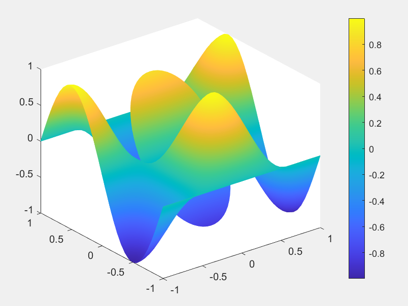
(a)

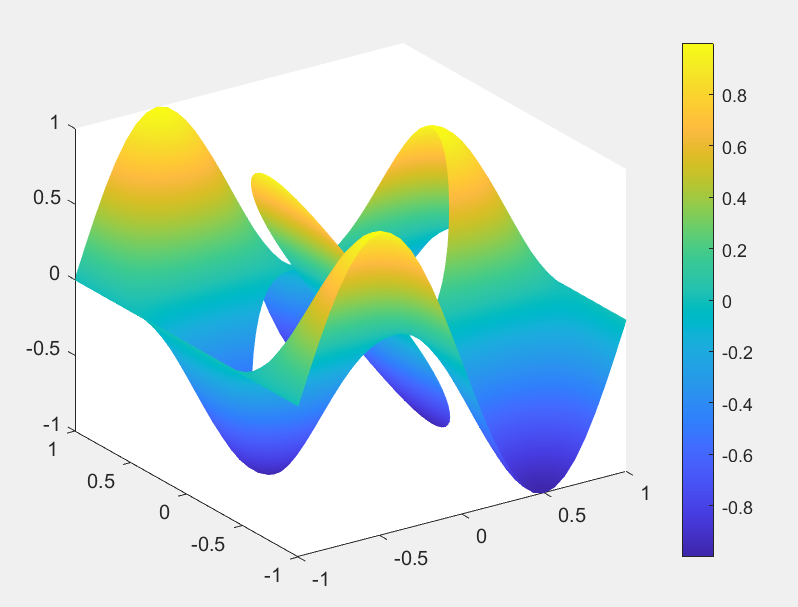
(b)

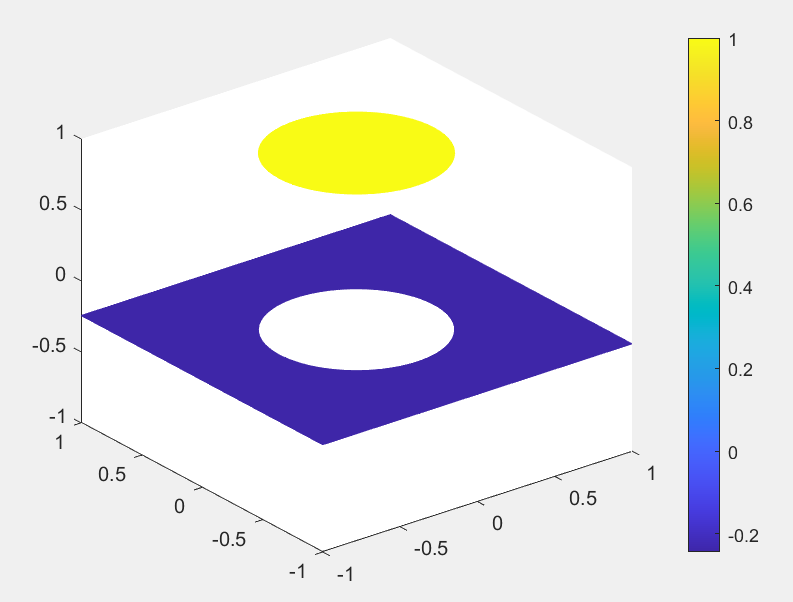
(c)

Fig. 2: Test problem 1: (a) x-component of ${\bf u}_{h}$, (b) y-component of ${\bf u}_{h}$, (c) pressure $p_{h}$

Table 2: Test Problem 1: straight triangular mesh

n	${|||}Q_{h}{\bf u}-{\bf u}_{h}{|||}$	order	$\|Q_{0}{\bf u}-{\bf u}_{0}\|$	order	$\|\pi_{h}p-p_{h}\|$	order
			$k=1$
1	3.8965e+00	–	6.9519e$-$01	–	8.9801e$-$01	–
2	1.9151e+00	1.025	1.6636e$-$01	2.063	4.1484e$-$01	1.114
3	9.5547e$-$01	1.033	4.1203e$-$02	2.073	1.9548e$-$01	1.118
4	4.7758e$-$01	1.049	1.0277e$-$02	2.100	9.5744e$-$02	1.079
			$k=2$
1	1.0515e+00	–	1.4146e$-$01	–	2.1288e$-$01	–
2	2.7967e$-$01	1.911	2.2582e$-$02	2.647	6.4754e$-$02	1.717
3	7.4373e$-$02	1.968	4.2713e$-$03	2.474	2.0841e$-$02	1.684
4	2.0444e$-$02	1.953	9.5717e$-$04	2.262	7.0023e$-$03	1.649
			$k=3$
1	3.7183e$-$01	–	6.1249e$-$02	–	1.6822e$-$01	–
2	9.7064e$-$02	1.938	1.4642e$-$02	2.065	5.7458e$-$02	1.549
3	2.9548e$-$02	1.767	3.6609e$-$03	2.059	1.9566e$-$02	1.600
4	9.6547e$-$03	1.692	9.1541e$-$04	2.096	6.7761e$-$03	1.604

In this test problem, we take discontinuous velocity ${\bf u}$ and discontinuous pressure $p$ in $\Omega$. The viscosity coefficient $A$ is continuous in $\Omega$. The numerical solutions are plotted in Fig 2. We perform the weak Galerkin approximation on the curved triangular mesh in Table 1 and the approximation performance on the straight triangular mesh in Table 2. The convergency rates on the curved triangular mesh for linear and high order weak Galerkin finite elements arrive at the optimal convergence order, but the convergence rates on the straight triangular mesh are less than or equal to second order. This results show the advantages for using curved element.

7.2 Test Problem 2

In the test problem 2, we consider the following problem with discontinuous velocity and the following interface:

$$r=\frac{1}{7}+\frac{sin(5\theta)}{7}.$$

The exact solutions are

$${\bf u}_{1} = \left(\begin{array}[]{ccc}2\pi\sin(\pi x)\sin(\pi x)\cos(\pi y)\sin(\pi y)\\ -2\pi\sin(\pi x)\sin(\pi y)\cos(\pi x)\sin(\pi y)\end{array}\right),$$

$${\bf u}_{2} = \left(\begin{array}[]{ccc}x^{2}y^{2}+e^{-y}\\ -\frac{2}{3}xy^{3}+2-\pi\sin(\pi x)\end{array}\right).$$

$$p=\left\{\begin{array}[]{rcl}0&\mbox{in}&\Omega_{1}\\ 0&\mbox{in}&\Omega_{2}\end{array}\right.,A=\left\{\begin{array}[]{rcl}1&\mbox{in}&\Omega_{1}\\ 1&\mbox{in}&\Omega_{2}\end{array}\right..$$ (111)

Table 3: Test Problem 2: curved triangular mesh

n	${|||}Q_{h}{\bf u}-{\bf u}_{h}{|||}$	order	$\|Q_{0}{\bf u}-{\bf u}_{0}\|$	order	$\|\pi_{h}p-p_{h}\|$	order
			$k=1$
1	7.5998e+00	–	6.1090e$-$01	–	1.0485e+00	–
2	4.3216e+00	0.808	1.7597e$-$01	1.781	6.4828e$-$01	0.688
3	2.4397e+00	0.913	4.7169e$-$02	2.104	3.7369e$-$01	0.881
4	1.4359e+00	0.771	1.3842e$-$02	1.784	1.7892e$-$01	1.072
			$k=2$
1	1.7074e+00	–	1.0609e$-$01	–	1.9216e$-$01
2	4.9432e$-$01	1.774	1.5831e$-$02	2.722	4.4089e$-$02	2.107
3	1.3598e$-$01	2.063	2.1676e$-$03	3.178	1.2716e$-$02	1.987
4	3.8032e$-$02	1.854	2.9822e$-$04	2.886	3.3685e$-$03	1.933

Table 4: Test Problem 2: curved quadrilateral mesh

n	${|||}Q_{h}{\bf u}-{\bf u}_{h}{|||}$	order	$\|Q_{0}{\bf u}-{\bf u}_{0}\|$	order	$\|\pi_{h}p-p_{h}\|$	order
			$k=1$
1	9.49922875	0	0.94464858	0	2.31404706	0
2	5.29716221	1.095023	0.24508676	2.529633	0.9827431	1.605685
3	2.92565833	0.937768	0.06320311	2.140848	0.374679	1.523232
4	1.64254865	0.869815	0.01863667	1.840104	0.22641591	0.758955
			$k=2$
1	2.83197438	0	0.19342218	0	0.33608256	0
2	0.75110962	2.488342	0.02719008	3.678621	0.0986695	2.297857
3	0.20086084	2.083476	0.00348692	3.244359	0.02366012	2.255731
4	0.05239902	2.024687	0.00044515	3.101487	0.00489772	2.373199

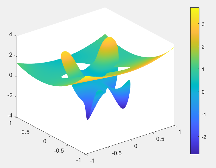
(a)

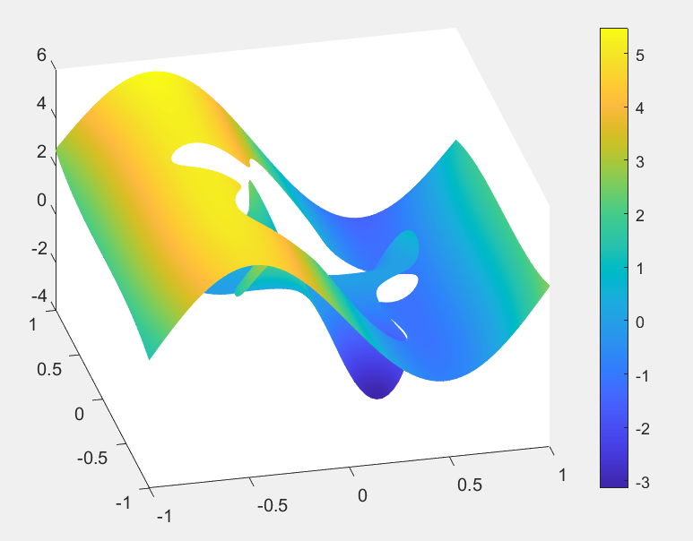
(b)

(c)

Fig. 3: Test problem 2: (a) x-component of ${\bf u}_{h}$, (b) y-component of ${\bf u}_{h}$, (c) pressure $p_{h}$

In this test problem, we consider a velocity function $\mathbf{u}$ that exhibits discontinuities within the domain $\Omega$. Meanwhile, the pressure $p$ and viscosity coefficient $A$ remain continuous throughout $\Omega$. The numerical solutions are depicted in Figure 3 and corresponding outcomes on triangular meshes and quadrilateral meshes are documented in Table 3 and Table 4 . The obtained results demonstrate that both linear and high-order weak Galerkin finite element methods achieve the expected convergence rates on the curved triangular mesh, reaching the optimal convergence order.

7.3 Test Problem 3

In the test problem 3, we consider the following problem and the following interface:

$$r=\frac{1}{2}+\frac{sin(2\theta)}{4}.$$

The exact solutions are

$${\bf u}_{1} = \left(\begin{array}[]{ccc}2\pi\sin(\pi x)\sin(\pi x)\cos(\pi y)\sin(\pi y)\\ -2\pi\sin(\pi x)\sin(\pi y)\cos(\pi x)\sin(\pi y)\end{array}\right),$$

$${\bf u}_{2} = \left(\begin{array}[]{ccc}x^{2}y^{2}+e^{-y}\\ -\frac{2}{3}xy^{3}+2-\pi\sin(\pi x)\end{array}\right),$$

$$p=\left\{\begin{array}[]{rcl}0&\mbox{in}&\Omega_{1}\\ 0&\mbox{in}&\Omega_{2}\end{array}\right.,A=\left\{\begin{array}[]{rcl}1&\mbox{in}&\Omega_{1}\\ 10&\mbox{in}&\Omega_{2}\end{array}\right..$$ (118)

Table 5: Test Problem 3: curved triangular mesh

n	${|||}Q_{h}{\bf u}-{\bf u}_{h}{|||}$	order	$\|Q_{0}{\bf u}-{\bf u}_{0}\|$	order	$\|\pi_{h}p-p_{h}\|$	order
			$k=1$
1	36.3891e$-$00	–	3.3882e$-$00	–	6.0909e$-$00	–
2	19.4433e$-$00	0.861	9.3543e$-$01	1.767	3.1101e$-$00	0.923
3	10.0110e$-$00	1.047	2.4362e$-$00	2.123	1.2411e$-$00	1.449
4	5.1226e$-$00	1.064	6.2217e$-$02	2.168	5.4089e$-$01	1.319
			$k=2$
1	4.6309e$-$00	–	3.3576e$-$01	–	5.3342e$-$01
2	1.2513e$-$00	1.797	4.5818e$-$02	2.735	1.1136e$-$02	2.151
3	3.1816e$-$01	2.160	5.8369e$-$03	3.251	2.4023e$-$02	2.419
4	8.1714e$-$02	2.159	7.4753e$-$04	3.264	5.8022e$-$03	2.256
			$k=3$
1	4.5929e-01	–	2.7574e$-$02	–	4.1069e$-$02	–
2	6.6604e-02	2.651	1.9988e$-$03	3.603	5.8208e$-$03	2.683
3	8.9622e-03	3.165	1.3464e$-$04	4.256	6.1539e$-$04	3.545
4	1.2440e-03	3.136	9.2808e$-$06	4.247	8.6033e$-$05	3.124

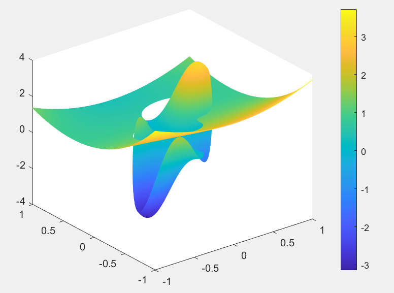
(a)

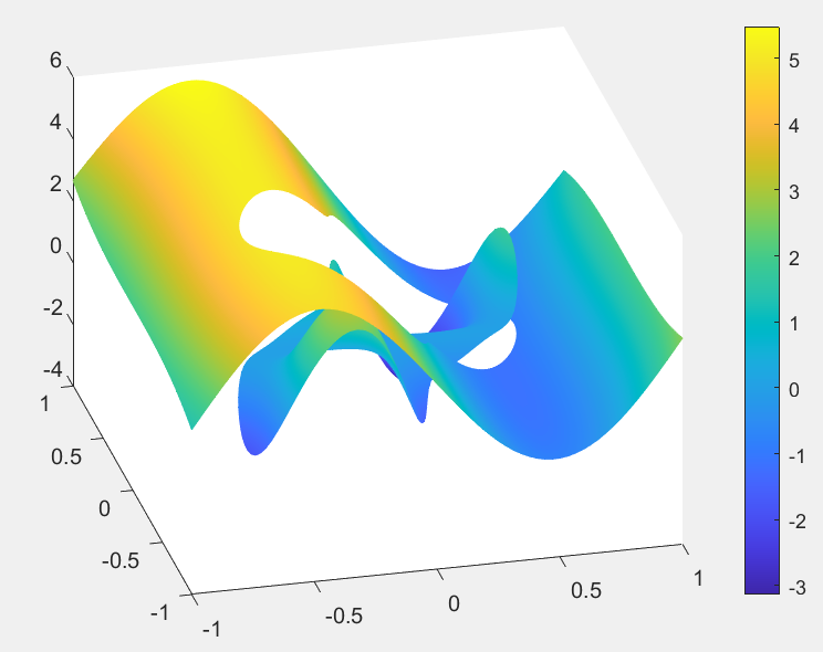
(b)

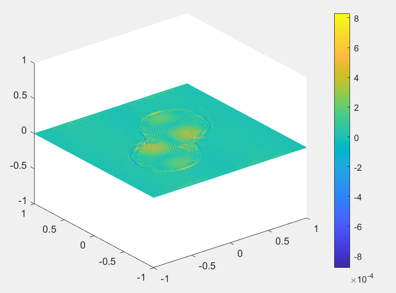
(c)

Fig. 4: Test problem 3: (a) x-component of ${\bf u}_{h}$, (b) y-component of ${\bf u}_{h}$, (c) pressure $p_{h}$

Table 6: Test Problem 3: curved quadrilateral mesh

n	${|||}Q_{h}{\bf u}-{\bf u}_{h}{|||}$	order	$\|Q_{0}{\bf u}-{\bf u}_{0}\|$	order	$\|\pi_{h}p-p_{h}\|$	order
			$k=1$
1	5.7446E+01	0.0000	8.7567E+00	0.0000	1.2942E+01	0.0000
2	2.9245E+01	1.0129	1.9566E+00	2.2484	1.1137E+01	0.2252
3	1.5191E+01	0.9911	4.2467E-01	2.3114	6.9653E+00	0.7102
4	7.8662E+00	1.1163	9.8041E-02	2.4866	3.0210E+00	1.4170
			$k=2$
1	7.6542E+00	0.0000	7.6482E-01	0.0000	2.3754E+00	0.0000
2	2.0451E+00	1.9801	1.0380E-01	2.9964	7.4628E-01	1.7371
3	5.2785E-01	2.0493	1.3457E-02	3.0911	1.9669E-01	2.0177
4	1.3549E-01	2.3068	1.7219E-03	3.4876	4.4093E-02	2.5364
			$k=3$
1	1.4042E+00	0.0000	1.2467E-01	0.0000	2.1995E-01	0.0000
2	1.6560E-01	3.2071	7.3189E-03	4.2537	2.3673E-02	3.3443
3	2.1098E-02	3.1175	4.7044E-04	4.1527	2.9584E-03	3.1467
4	2.7359E-03	3.4649	3.0588E-05	4.6359	3.7633E-04	3.4975

In this test problem, we consider the utilization of a discontinuous velocity function ${\bf u}$ and a viscosity coefficient $A$. The pressure function $p$ is assumed to be continuous throughout the domain $\Omega$. The obtained numerical solutions are illustrated in Figure 4. The results of the weak Galerkin finite element method on triangular meshes and quadrilateral meshes are presented in Table 5 and 6 respectively. The results demonstrate that both linear and high-order weak Galerkin finite element methods attain the desired optimal convergence rates.

8 Conclusion

In this paper, we use the weak Galerkin finite element method to deal with Stokes interface problems with complex interface. We present a weak Galerkin finite element numerical scheme with two values at the interface. It is proved that the optimal convergence order can be reached under the energy norm and the $L^{2}$ norm. At the same time, the results of numerical examples also show that the error convergence order under the energy norm and $L^{2}$ norm is optimal, which is consistent with the theory.

References

- [1] I. Babuska, B. A. Szabo, and I. N. Katz, The p-version of the finite element method, Siam. J. Numer. Anal., 18 (1981), pp. 515–545.
- [2] S. C. Brenner and L. R. Scott, The mathematical theory of finite element methods, Texts in Applied Mathematics, Springer-Verlag, New York, 2002.
- [3] F. Brezzi and M. Fortin, Mixed and hybrid finite element methods, Springer Series in Computational Mathematics, Springer-Verlag, New York, 1991.
- [4] W. Chen, F. Wang, and Y. Wang, Weak Galerkin method for the coupled Darcy-Stokes flow, IMA J. Numer. Anal., 36 (2016), pp. 897–921.
- [5] E. V. Chizhonkov, Numerical solution to a stokes interface problem, Comput. Math. and Math. Phys., 49 (2009), pp. 105–116.
- [6] M. Crouzeix and P.-A. Raviart, Conforming and nonconforming finite element methods for solving the stationary Stokes equations. I, Rev. Française Automat. Informat. Recherche Opérationnelle Sér. Rouge, 7 (1973), pp. 33–75.
- [7] V. Giraud and P. Raviart, Finite Element Methods for the Navier-Stokes Equations, Theory and Algorithms, Springer Series in Computational Mathematics, Springer Berlin, 1986.
- [8] P. P. Grinevich and M. A. Olshanskii, An iterative method for the Stokes-type problem with variable viscosity, SIAM J. Sci. Comput., 31 (2009), pp. 3959–3978.
- [9] Q. Guan, Weak galerkin finite element method for second order problems on curvilinear polytopal meshes with lipschitz continuous edges or faces, 2019.
- [10] M. D. Gunzburger, Finite element methods for viscous incompressible flows, Computer Science and Scientific Computing, Academic Press, Inc., Boston, MA, 1989.
- [11] P. Kagan, A. Fischer, and P. Z. Bar-Yoseph, New b-spline finite element approach for geometrical design and mechanical analysis, Int. J. Numer. Meth. Eng., 41 (1998), pp. 435–458.
- [12] Y. Liu, W. Chen, and Y. Wang, A weak Galerkin mixed finite element method for second order elliptic equations on 2D curved domains, Commun. Comput. Phys., 32 (2022), pp. 1094–1128.
- [13] L. Mu, Numerical analysis for interface problems, ProQuest LLC, Ann Arbor, MI, 2012. Thesis (Ph.D.)–University of Arkansas at Little Rock.
- [14] , Weak Galerkin finite element with curved edges, J. Comput. Appl. Math., 381 (2021), p. 113038.
- [15] L. Mu, J. Wang, and X. Ye, A stable numerical algorithm for the Brinkman equations by weak Galerkin finite element methods, J. Comput. Phys., 273 (2014), pp. 327–342.
- [16] L. Mu, J. Wang, X. Ye, and S. Zhao, A new weak Galerkin finite element method for elliptic interface problems, J. Comput. Phys., 325 (2016), pp. 157–173.
- [17] M. A. Olshanskii and A. Reusken, Analysis of a Stokes interface problem, Numer. Math., 103 (2006), pp. 129–149.
- [18] H. Peng, Q. Zhai, R. Zhang, and S. Zhang, A weak Galerkin-mixed finite element method for the Stokes-Darcy problem, Sci. China Math., 64 (2021), pp. 2357–2380.
- [19] D. W. Schmid and Y. Y. Podladchikov, Analytical solutions for deformable elliptical inclusions in general shear, Geophys. J. Int., 155 (2003), pp. 269–288.
- [20] R. Sevilla, S. Fernández-Méndez, and A. Huerta, NURBS-enhanced finite element method for Euler equations, Internat. J. Numer. Methods Fluids, 57 (2008), pp. 1051–1069.
- [21] R. Sevilla, S. Fernández-Méndez, and A. Huerta, NURBS-enhanced finite element method (NEFEM), Internat. J. Numer. Methods Engrg., 76 (2008), pp. 56–83.
- [22] B. Szabó and I. Babuška, Finite element analysis, A Wiley-Interscience Publication, John Wiley & Sons, Inc., New York, 1991.
- [23] V. P. Trubitsyn, A. A. Baranov, A. Eyseev, and A. Trubitsyn, Exact analytical solutions of the stokes equation for testing the equations of mantle convection with a variable viscosity, IZV-PHYS SOLID EART+., 42 (2006), pp. 537–545.
- [24] C. Wang, J. Wang, R. Wang, and R. Zhang, A locking-free weak Galerkin finite element method for elasticity problems in the primal formulation, J. Comput. Appl. Math., 307 (2016), pp. 346–366.
- [25] J. Wang and X. Ye, A weak Galerkin finite element method for second-order elliptic problems, J. Comput. Appl. Math., 241 (2013), pp. 103–115.
- [26] , A weak Galerkin mixed finite element method for second order elliptic problems, Math. Comp., 83 (2014), pp. 2101–2126.
- [27] , A weak Galerkin finite element method for the stokes equations, Adv. Comput. Math., 42 (2016), pp. 155–174.
- [28] X. Wang, Q. Zhai, and R. Zhang, The weak Galerkin method for solving the incompressible Brinkman flow, J. Comput. Appl. Math., 307 (2016), pp. 13–24.
- [29] D. Xue and L. Demkowicz, Control of geometry induced error in finite element (FE) simulations. I. Evaluation of FE error for curvilinear geometries, Int. J. Numer. Anal. Model., 2 (2005), pp. 283–300.
- [30] Q. Zhai, R. Zhang, and X. Wang, A hybridized weak Galerkin finite element scheme for the Stokes equations, Sci. China Math., 58 (2015), pp. 2455–2472.
- [31] H. Zhang, Y. Zou, Y. Xu, Q. Zhai, and H. Yue, Weak Galerkin finite element method for second order parabolic equations, Int. J. Numer. Anal. Model., 13 (2016), pp. 525–544.
- [32] M. Zlámal, Curved elements in the finite element method. I, SIAM J. Numer. Anal., 10 (1973), pp. 229–240.
- [33] , Curved elements in the finite element method. II, SIAM J. Numer. Anal., 11 (1974), pp. 347–362.