Decision-making with Imaginary Opponent Models

Abstract

Opponent modeling has benefited a controlled agent’s decision-making by constructing models of other agents. Existing methods commonly assume access to opponents’ observations and actions, which is infeasible when opponents’ behaviors are unobservable or hard to obtain. We propose a novel multi-agent distributional actor-critic algorithm to achieve imaginary opponent modeling with purely local information (i.e., the controlled agent’s observations, actions, and rewards). Specifically, the actor maintains a speculated belief of the opponents, which we call the imaginary opponent models, to predict opponents’ actions using local observations and makes decisions accordingly. Further, the distributional critic models the return distribution of the policy. It reflects the quality of the actor and thus can guide the training of the imaginary opponent model that the actor relies on. Extensive experiments confirm that our method successfully models opponents’ behaviors without their data and delivers superior performance against baseline methods with a faster convergence speed.

Introduction

Recently, there has been a growing effort in applying multi-agent reinforcement learning (MARL) to address the complex learning tasks in multi-agent systems, including cooperation, competition, and a mix of both (Hernandez-Leal, Kartal, and Taylor 2019; Zhang, Yang, and Başar 2021). To help the controlled agent build knowledge of other agents, most existing works normally consider the opponents as a part of environment and naively feed the observations and actions of other agents to the controlled agent during training (Lowe et al. 2017; Foerster et al. 2018b; Rashid et al. 2018; Wei et al. 2018). However, other people argue that the controlled agent should be endowed with abilities to reason about other agents’ unknown goals and behaviors, thus coming up with opponent modeling (Albrecht and Stone 2018). Although there is already a considerable amount of research devoted to this opponent modeling problem, existing works commonly assume free access to opponents’ information (He et al. 2016; Foerster et al. 2018a; Raileanu et al. 2018; Tian et al. 2019; Papoudakis, Christianos, and Albrecht 2021). These canonical methods use the opponents’ observations and actions as the ground truth during the training of opponent models. However, the access to opponents’ real observations and actions may not be available or cheap in many cases. For instance, even in a simulator that the user has complete control, the opponent’s policy can come from third-party resources and thus, its observation format is unknown. When it comes to realistic training environments, even we have the full knowledge of opponents’ configuration, collecting the opponents’ running data induces high costs as the number of agents and the task complexity increase. In these cases, the agent must model its opponents with only locally available information (i.e., its own observations, actions, and rewards) if it wants to benefit from opponent modeling, which seems counter-intuitive. Thus, a natural question that comes to mind is: can we portray the opponents’ behaviors with purely local information?

This study proposes a speculation-based adversary modeling of the opponents, which we call the imaginary opponent models, to predict opponents’ actions using local observations. In our algorithm, the agent maintains one imaginary opponent model for each opponent, which receives the local information to predict the unknown opponent policy. At each time step, these opponent models take the agent’s observation as input and output the action probability distributions that represent the estimated opponents’ behavior. Based on these distributions, the agent samples multiple opponent joint actions, each of which is fed into the actor to output an action probability distribution for the agent. The final action probability distribution of the agent is the sum of the actor’s outputs weighted by the probability of corresponding opponent joint action. By this design, the agent policy is deeply coupled with the opponent models. We expect that a better opponent model can improve the decision quality because it provides the actor with more accurate information about the opponents. Therefore, it is possible to use the quality of agent policy as one kind of feedback to train the opponent models. This is the key insight of our work. To gather as much feedback as possible, we propose to use the distributional critic (Bellemare, Dabney, and Munos 2017; Dabney et al. 2018b) to model the return distribution of the agent policy. Compared to an expected return, the return distribution can provide more information. We wrap the opponent model aided actor and distributional critic as our multi-agent actor-critic framework to achieve opponent modeling with local information. To summarize, we highlight the following contributions: (i) To the best of our knowledge, this is the first work to achieve the opponent modeling with purely local information for MARL. (ii) This is the first work that sheds the light on the potential of distributional critic for guiding the training of opponent models, which can encourage future researches. (iii) We formally derive the policy gradient and opponent model gradient and propose a practical algorithm to train the actor and critic effectively. (iv) We evaluate the proposed method in different multi-agent environments. The evaluation confirms that our method successfully models reliable opponents’ policy without their data and achieves better performance with a faster convergence speed than baselines.

Related work

Opponent modeling. Opponent modeling is a research topic that emerged alongside the game theory (Brown 1951). With the powerful representation capabilities of recent deep learning architectures, opponent modeling has ushered in significant progress (Albrecht and Stone 2018). Type-based reasoning methods (He et al. 2016; Hong et al. 2018; Raileanu et al. 2018; Albrecht and Stone 2017) assume that the opponent has one of several known types and update the belief using their observations obtained during training. Recursive reasoning methods (Rabinowitz et al. 2018; Yang et al. 2019; Zheng et al. 2018; Wen et al. 2019; Zintgraf et al. 2021) model the beliefs about the mental states of other agents via deep neural networks. Other approaches (Tian et al. 2019; Liu et al. 2019) regularize opponent modelling with novel objectives. However, the aforementioned works commonly assume access to the opponents’ observations and actions during both training and execution. Recent researches (Papoudakis, Christianos, and Albrecht 2020, 2021) argue that the access to opponents’ observations and actions during execution is often infeasible (e.g., in large-scale applications). They propose to learn an opponent model that only uses agents’ local information and thus, eliminate the need of opponents’ information during execution. However, their approaches still require the opponents’ true information during training. Thus, how to model an opponent’s policy when its information is unavailable during training is still an open problem. Our work presents the first attempt to solve this challenging problem.

Distributional reinforcement learning. Distributional reinforcement learning (RL) aims to model the return distributions rather than the expected return, and use these distributions to evaluate and optimize a policy (Bellemare, Dabney, and Munos 2017; Dabney et al. 2018a, b). Many studies have shown that distribution RL can achieve better performance than the state-of-art methods from the classical RL (Barth-Maron et al. 2018; Tessler, Tennenholtz, and Mannor 2019; Singh, Lee, and Chen 2020; Yue, Wang, and Zhou 2020). Motivated by the successes in single-agent scenarios, several studies (Lyu and Amato 2020; Hu et al. 2020) have extended the distributional RL method to multi-agent settings. They have used the distributional RL to alleviate the instability issue resulting from the exploration of other learning agents during training. Our work uses distributional RL to evaluate the quality of the agent policy and thus, guide the training of the opponent model that the policy relies on. Together with previous works, we show the great potential of distributional RL and can attract more research efforts to this area.

Preliminary

Partially observable Markov games. A partially observable Markov game (POMG) (Lowe et al. 2017) of $n$ agents is formulated as a tuple $\mathcal{M}=\langle\mathcal{S},\mathbb{O},\mathcal{O},\mathcal{A},\mathcal{T},\mathcal{R},\gamma\rangle$. $\mathcal{S}$ is a set of states describing the possible configuration of all agents and the external environment. Also, each agent $i$ has its own observation space $\mathbb{O}_{i}\in\mathbb{O}$. Due to the partial observability, in every state $s\in\mathcal{S}$, each agent $i$ gets a correlated observation $o_{i}$ based on its observation function $\mathcal{O}_{i}:\mathcal{S}\rightarrow\mathbb{O}_{i}$ where $\mathcal{O}_{i}\in\mathcal{O}$. The agent $i$ selects an action $a_{i}\in A_{i}$ from its own action space $A_{i}\in\mathcal{A}$ at each time step, giving rise to a joint action $[a_{1},\cdots,a_{n}]\in A_{1}\times A_{2}\times\cdots\times A_{n}$. The joint action then produces the next state by following the state transition function $\mathcal{T}:\mathcal{S}\times A_{i}\times\cdots\times A_{n}\rightarrow\mathcal{S}$. $\mathcal{R}=\{r_{i}\}$ is the set of reward functions. After each transition, agent $i$ receives a new observation and obtains a scalar reward as a function of the state and its action $r_{i}:\mathcal{S}\times A_{i}\rightarrow\mathbb{R}$. The initial state $s\in\mathcal{S}$ is determined by some prior distribution $p:\mathcal{S}\rightarrow[0,1]$. Each agent $i$ aims to maximize its own total expected return $R_{i}=\mathbb{E}_{r^{t}\sim r_{i}(s_{t},a_{i}^{t}),(s_{t},a_{i}^{t})\sim\tau}\sum_{t=0}^{T}\gamma^{t}r^{t}$, where $\gamma$ is the discount factor, $r^{t}$ is its sampled reward at time step $t$, $\tau$ is the trajectory distribution induced by the joint policy of all agents, and $T$ is the time horizon. Without loss of generality, we assume that the $n$ agent can be divided into $|M|\leq n$ teams, and each team has $q$ agents with $1\leq q\leq n$. We consider the other teams as opponent agents which are controlled by a set of fixed policies. Note that a single agent can also form a team. We assume agents from the same team fully cooperate and thus share the same reward function.

Actor-Critic method. The actor-critic algorithm (Konda and Tsitsiklis 2000) is a subclass of policy gradient methods (Silver et al. 2014). It has been widely used for tackling complex tasks. The algorithm consists of two components. The $critic$ $Q_{\phi}^{\pi}$ estimates the true action-value function $Q^{\pi}(s,a)$ that represents the expected return of taking action $a$ in state $s$ and then following policy $\pi$. It adjusts the parameters $\phi$ with an appropriate policy evaluation algorithm such as temporal-difference learning (Sutton and Barto 2018). With the critic, the $actor$ adjusts the parameter $\theta$ of the agent’s policy $\pi_{\theta}$ by applying the policy gradient theorem (Sutton et al. 2000):

$$\nabla_{\theta}J(\theta)=\mathbb{E}_{\pi_{\theta}}[\nabla_{\theta}\log\pi_{\theta}(a|s)Q_{\phi}^{\pi}(s,a)].$$ (1)

In the multi-agent scenarios, the actor-critic algorithm is applied to learn optimal policy for each agent. To stabilize the training, the common approach is to follow the centralized training and decentralized execution (CTDE) setting (Hernandez-Leal, Kartal, and Taylor 2019), where it commonly assumes that the agent $i$’s action-value function $Q_{i}^{\pi_{i}}(o_{1},\dots,o_{n},a_{1},\dots,a_{n})$ takes as input the joint observations and joint actions.

Distributional reinforcement learning. Unlike traditional RL whose target is to maximize the expected total return, distributional RL (Bellemare, Dabney, and Munos 2017) explicitly considers the randomness of the return distribution. The expected discounted return $Q^{\pi}$ can be written as:

$$Q^{\pi}(s,a)=\mathbb{E}[Z^{\pi}(s,a)]=\mathbb{E}[\sum_{t=0}^{\infty}\gamma^{t}r(s_{t},a_{t})],$$ (2)

where $s_{t}\sim P(\cdot|s_{t-1},a_{t-1}),a_{t}\sim\pi(\cdot|s_{t}),s_{0}=s,a_{0}=a$. $Z^{\pi}(s,a)$ is the return distribution, covering all sources of intrinsic randomness including reward function, state transition, stochastic policy sampling, and systematic stochasticity. In the distributional RL, we directly model the random return $Z^{\pi}(s,a)$ instead of its expectation. The distributional Bellman equation can be defined as,

$$Z(s,a)\overset{D}{=}r(s,a)+\gamma P^{\pi}Z(s,a),$$ (3)

where $\overset{D}{=}$ means the two sides of the equation are distributed according to the same law, $P^{\pi}Z(s,a)\overset{D}{=}Z(S^{\prime},A^{\prime})$ and $S^{\prime}\sim P(\cdot|s,a)$, $A^{\prime}\sim\pi(\cdot|S^{\prime})$.

Methodology

The overall framework

Our training follows the CTDE setting, i.e., we have the access to the observations and actions of the team we control. Note that, however, we do not know the observations and actions of the opponent team during the training. Figure 1 depicts the overall framework of the proposed distributional opponent model aided actor-critic (DOMAC) algorithm.

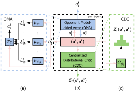
Figure 1: The DOMAC framework.

In DOMAC, each controlled agent $i$ has two components, the opponent model aided actor (OMA) (Figure 1(a)), and a centralized distributional critic (CDC) (Figure 1(c)). Suppose the agent $i$ has total $p$ opponents in the game. It models them by $p$ imaginary opponent models, each corresponding to one of the opponents. For example, in Figure 1(a), $\mu_{\psi_{ik}}$ is the imaginary opponent model for the opponent $k$ ($1\leq k\leq p$). The local information refers to the observation, action and reward of agent $i$. Once the agent $i$ receives a local observation, $o^{t}_{i}$ at time step $t$, each of its opponent models receive as input $o^{t}_{i}$, in addition to their ID. After processing, $\mu_{\psi_{ik}}$ outputs a distribution over the corresponding opponent $k$’s action space. From this distribution, the agent $i$ can sample the opponent $k$’s predicted action $\hat{a}^{t}_{ik}$. Then the agent policy $\pi_{\theta_{i}}$ takes the joint predicted action $\hat{a}^{t}_{i}=[\hat{a}^{t}_{i1},\dots,\hat{a}^{t}_{ip}]$ together with the observation $o^{t}_{i}$ as input, and outputs a distribution over agent $i$’s own action space $A_{i}$. Note that each sampled $\hat{a}^{t}_{i}$ results in one action probability distribution of the agent $i$. We conduct the sampling process for multiple times and aggregate the resulting action probability distributions into one final distribution from which the action $a^{t}_{i}$ is sampled.

After all agents in the controlled team sample their actions, each controlled agent $i$’s CDC network $G_{\phi_{i}}$ takes as input the joint observation $\mathbf{o}^{t}$ and joint action $\mathbf{a}^{t}$ of its team, and computes a return distribution $Z_{i}(\mathbf{o}^{t},\mathbf{a}^{t})$. Note that each agent in the controlled team has an independent set of OMA and CDC, and the only shared are their observations and actions. This is critical for extracting the individual knowledge of each agent which may be heterogeneous for their different observations, current statuses, etc. In general, the rationales of DOMAC can be explained as the same closed optimization loop like that of the original actor-critic framework. OMA receives the local information with the beliefs of modeled opponents (i.e., predicted opponents’ actions). It improves the decision-making by adjusting opponent models and actively selecting the actions with higher evaluations according to CDC, while CDC, in turn, evaluates the improved policy. In the following, we first show that optimizing the OMA can be formulated as a policy gradient theorem. Then we formulate the optimization of CDC by using a quantile regression loss. Finally, we transform the theoretical findings into a concrete algorithm presented in Algorithm 1.

Opponent model aided actor

In this section, we discuss the theoretical aspect of the OMA in details. For clarity, we omit time step $t$ in all formulas below. Let $\mu_{\psi_{ik}}$ and $\pi_{\theta_{i}}$ be parameterized with the trainable parameters $\psi_{ik}$ and $\theta_{i}$, respectively, and $\psi_{i}=\{\psi_{ik}\}$ be the set of parameters of all imaginary opponent models maintained by the agent $i$. Given an observation $o_{i}$, the OMA of agent $i$ calculates its action probability distribution as:

$$\rho_{\theta_{i},\psi_{i}}(a_{i}|o_{i}) =\sum_{\hat{a}_{i}}[\pi_{\theta_{i}}(a_{i}|\hat{a}_{i},o_{i})P(\hat{a}_{i}|o_{i})]$$

$$=\sum_{\hat{a}_{i}}[\pi_{\theta_{i}}(a_{i}|\hat{a}_{i},o_{i})\prod_{k=1}^{p}\mu_{\psi_{ik}}(\hat{a}_{ik}|o_{i})],$$ (4)

where $\hat{a}_{i}=[\hat{a}_{i1},\dots,\hat{a}_{ip}]\in\hat{A}_{i}$. Here we assume that each imaginary opponent model is independent with each other. Then, the objective of agent $i$ is to maximize its total expected return, which is determined by the parameters $\theta_{i}$ and $\psi_{i}$:

$$J(\theta_{i},\psi_{i})=\mathbb{E}_{\mathbf{o}\sim\tau,a_{i}\sim\rho_{\theta_{i},\psi_{i}}}[\mathbb{E}(Z_{i}(\mathbf{o},\mathbf{a}))],$$ (5)

where $(\mathbf{o},\mathbf{a})$ represents the joint observation and joint action of the agent $i$’s team, and $\tau$ represents the trajectory distribution induced by all agents’ policies. Additionally, we add the entropy of the policy into the objective function (5) to ensure an adequate exploration, which is proved to be effective for improving the agent performance (Mnih et al. 2016). Thus, the OMA’s final objective can be defined as:

$$J(\theta_{i},\psi_{i})=\mathbb{E}_{\mathbf{o},a_{i}}[\mathbb{E}(Z_{i}(\mathbf{o},\mathbf{a}))-\alpha_{i}\log\rho_{\theta_{i},\psi_{i}}(a_{i}|o_{i})],$$ (6)

where $\alpha_{i}$ is a hyperparameter controlling the degree of exploration. Next, we mathematically derive the closed form of the policy gradient and opponent model gradient respectively, which is summarized in the following proposition.

Proposition 0.1.

In a POMG, under the opponent modeling framework defined, the gradient of parameters $\theta_{i}$ for the policy of agent $i$ is given as:

$$\begin{split}\nabla_{\theta_{i}}J(\theta_{i},\psi_{i})&=\mathbb{E}_{\rho_{\theta_{i},\psi_{i}}}\Bigl{[}\nabla_{\theta_{i}}\log(\rho_{\theta_{i},\psi_{i}})\cdot\\ &[\mathbb{E}(Z_{i})-\alpha_{i}\log(\rho_{\theta_{i},\psi_{i}})-\alpha_{i}]\Bigr{]},\end{split}$$ (7)

and the gradient of the parameters $\psi_{ik}$ for the opponent model $\mu_{\psi_{ik}}$ is given as:

$$\begin{split}\nabla_{\psi_{ik}}J(\theta_{i},\psi_{i})&=\mathbb{E}_{\rho_{\theta_{i},\psi_{i}}}\Bigl{[}\nabla_{\psi_{ik}}\log(\rho_{\theta_{i},\psi_{i}})\cdot\\ &[\mathbb{E}(Z_{i})-\alpha_{i}\log(\rho_{\theta_{i},\psi_{i}})-\alpha_{i}]\Bigr{]},\end{split}$$ (8)

where $\rho_{\theta_{i},\psi_{i}}$ is defined in Equation (4).

Please refer to Appendix for the details of the proof. In general, the policy gradient (7) and opponent model gradient (8) both follow the format of policy gradient theorem (Sutton et al. 1999). This proposition states that OMA can adjust the parameters $\theta_{i}$ and $\psi_{i}$ towards maximizing the objective by following the gradient. Intuitively speaking, the OMA directly search the optimal policy and reliable opponent models by looking at the agent’s objective, which does not require the access to opponents’ true information. Although it may looks weak to use the objective as the only signal, we will show that the gradient of the objective is already sufficient for training reliable opponent models and thereby good actors.

Centralized distributional critic

To enhance training and provide a more delicate evaluation of the OMA, we adopt a distributional perspective to evaluate agents’ performance by modeling their return distributions (Bellemare, Dabney, and Munos 2017). We propose to learn a centralized distributional critic (CDC) for each controlled agent $i$. Following (Dabney et al. 2018b), we train the CDC with the quantile regression technique. Specifically, we implement the CDC for the agent $i$ as a deep neural network $G_{\phi_{i}}$ with $\phi_{i}$ being the trainable parameters. Given the joint observations and joint actions $(\mathbf{o},\mathbf{a})$ of agent $i$’s team, $G_{\phi_{i}}$ outputs a $K$-dimensional vector $\{G_{\phi_{i}}^{j}(\mathbf{o},\mathbf{a})\}_{j=1,\cdots,K}$. The elements of this output are the samples that approximate the agent $i$’s return distribution $Z_{i}(\mathbf{o},\mathbf{a})$. That is, we can represent the distribution approximation as $\frac{1}{K}\sum_{j=1}^{K}{\delta_{G_{\phi_{i}}^{j}(\mathbf{o},\mathbf{a})}}$ where $\delta_{z}$ denotes a Dirac at $z\in\mathbb{R}$. An ideal approximation can map these $K$ samples to $K$ fixed quantiles $\{\omega_{j}=\frac{j}{K}\}_{j=1,\cdots,K}$ so that $P(Z_{i}(\mathbf{o},\mathbf{a})\leq G_{\phi_{i}}^{j}(\mathbf{o},\mathbf{a}))=\omega_{j}$. To approach that, we compute the target distribution approximation $\hat{G}_{\phi_{i}}(\mathbf{o},\mathbf{a})$ based on the distributional Bellman operator,

$$\hat{G}_{\phi_{i}}(\mathbf{o},\mathbf{a})=\{r(s,\mathbf{a})+\gamma G_{\phi_{i}}^{j}(\mathbf{o}^{\prime},\mathbf{a}^{*})\}_{j=1,\cdots,K},$$ (9)

where $\mathbf{o}^{\prime}\sim\tau,\mathbf{a}^{*}=\arg\max_{\mathbf{a}^{\prime}}\mathbb{E}[G_{\phi_{i}}(\mathbf{o}^{\prime},\mathbf{a}^{\prime})].$ The objective of the CDC training then becomes minimizing the distance between $\hat{G}_{\phi_{i}}$ and $G_{\phi_{i}}$. To this end, we use the Quantile Huber loss (Dabney et al. 2018b),

$$\mathcal{L}_{QR}=\frac{1}{K^{2}}\sum_{j^{\prime}=1}^{K}\sum_{j=1}^{K}[\rho_{\omega_{j}}(\hat{G}_{\phi_{i}}^{j^{\prime}}(\mathbf{o},\mathbf{a})-G_{\phi}^{j}(\mathbf{o},\mathbf{a}))],$$ (10)

where $\rho_{\omega_{j}}(\mu)=|\omega_{j}-\mathbbm{1}_{\mu\leq 0}|\mathcal{L}_{\kappa}(\mu)$. $\mathbbm{1}_{\mu\leq 0}$ is an indicator function which means $\mathbbm{1}_{\mu\leq 0}=1$ when $\mu\leq 0$ else 0. $\kappa$ is a pre-fixed threshold, and the Huber loss is given by,

$$\mathcal{L}_{\kappa}(\mu)=\frac{1}{2}\mu^{2}\mathbbm{1}_{[|\mu|\leq\kappa]}+\kappa(|\mu|-\frac{1}{2}\kappa)\mathbbm{1}_{[|\mu|>\kappa]}.$$ (11)

Practical algorithm

We now present a tangible algorithm for training OMA and CDC. First, we introduce a sampling trick that is essential for the algorithm. According to Equation (4), computing the marginal distribution $\rho_{\theta_{i},\psi_{i}}$ can be exponentially costly concerning the dimensionality of the opponents’ action space. Formally, each agent $i$’s opponent $k$ has $|A_{ik}|$ actions. Then calculating the exact $\rho_{\theta_{i},\psi_{i}}$ requires traversing $|A_{i1}|\times\cdots\times|A_{ip}|$ combinations of opponents’ predicted actions, which quickly becomes intractable as $p$ increases. Therefore, in our algorithm, we apply a sampling trick that samples a set of actions $\hat{a}_{ik}=(\hat{a}_{ik1},\cdots,\hat{a}_{ikl})$ from the output of the imaginary opponent model $\mu_{\psi_{ik}}$ for each opponent $k$, where $l$ controls the size of sampled actions. Thus, $\rho_{\theta_{i},\psi_{i}}(a_{i}|o_{i})$ can be approximated as,

$$\bar{\rho}_{\theta_{i},\psi_{i}}(a_{i}|o_{i})=\sum_{l}\pi_{\theta_{i}}(a_{i}|o_{i},\{\hat{a}_{ikl}\})\prod_{k=1}^{p}\mu_{\psi_{ik}}(\hat{a}_{ikl}|o_{i}).$$ (12)

The action $a_{i}$ can be sampled from $\bar{\rho}_{\theta_{i},\psi_{i}}(a_{i}|o_{i})$ for each agent. We use empirical samples $\{G_{\phi_{i}}^{j}(\mathbf{o},\mathbf{a})\}_{j=1,\cdots,K}$ to approximate $Z_{i}(\mathbf{o},\mathbf{a})$. The objective function of OMA is,

$$J(\theta_{i},\psi_{i})=\mathbb{E}_{\mathbf{o},a_{i}}[\frac{1}{K}\sum_{j=1}^{K}G_{\phi_{i}}^{j}(\mathbf{o},\mathbf{a})-\alpha_{i}\cdot\log{\bar{\rho}}_{\theta_{i},\psi_{i}}(a_{i}|o_{i})].$$ (13)

We incorporate the proposed OMA and CDC into the on-policy framework. Generally speaking, the training procedure of DOMAC is similar to that of other on-policy multi-agent actor-critic algorithms (Foerster et al. 2018b), where the training data is generated on the fly. At each training iteration, the algorithm first generates training data with the current OMA and CDC. Then, we compute the objectives of OMA and CDC from the generated data, respectively. At last, the optimizer updates the parameters $\phi_{i}$, $\theta_{i}$, and $\psi_{i}$ accordingly. After that, the updated OMA and CDC are used in the next training iteration. In practice, we can parallelize the training, which is a common technique to reduce the training time (Iqbal and Sha 2019). In such case, the training data is collected from all parallel environments, and actions are sampled and executed in respective environment concurrently. We summarize the training procedure in Algorithm 1.

Algorithm 1 Training Procedure of DOMAC

1:A POMG environment env, a back-propagation optimizer Opt, number of episodes $E$, number of forward steps $T_{f}$, and $\pi_{\theta_{i}}$, $\mu_{\psi_{i}}$, $G_{\phi_{i}}$ with initialized parameters $\theta_{i}$, $\psi_{i}$, and $\phi_{i}$ for each agent $i$.

2:for $e$ =1, …, $E$ do

3:     $t\leftarrow 1$; Reset env to obtain initial observations $\mathbf{o}^{1}$.

4:     while env is not done do // Generate data

5:         for $t^{*}=t,\dots,t+T_{f}-1$  do

6:              Sample actions $\mathbf{a}^{t^{*}}$, where $a_{i}^{t^{*}}\in\mathbf{a}^{t^{*}}$

7:              follows $a_{i}^{t^{*}}\sim\rho_{\theta_{i},\psi_{i}}(a_{i}^{t^{*}}|o_{i}^{t^{*}})$.

8:              Execute $\mathbf{a}^{t^{*}}$ to obtain joint rewards $\mathbf{r}^{t^{*}}$

9:              and new observations $\mathbf{o}^{t^{*}+1}$.

10:              Store transition data $(\mathbf{o}^{t^{*}},\mathbf{a}^{t^{*}},\mathbf{r}^{t^{*}},\mathbf{o}^{t^{*}+1})$.

11:         end for

12:         for $1\leq i\leq n$ do // Update OMA, CDC

13:              Calculate $Z_{i}$, $\bar{\rho}_{\theta_{i},\psi_{i}}$ with collected data.

14:              Updates $G_{\phi_{i}}$ by minimizing Equation (10)

15:              Updates $\pi_{\theta_{i}}$ by minimizing Equation (13)

16:              Updates $\mu_{\psi_{i}}$ by minimizing Equation (13)

17:         end for

18:         $t\leftarrow t+T_{f}$.

19:     end while

20:end for

Experiments

To thoroughly assess our DOMAC algorithm, we test it in two partially observable multi-agent environments, namely the predator-prey environment (Koul 2019; Böhmer, Kurin, and Whiteson 2020) and the pommerman environment (Resnick et al. 2018). We design multiple Markov games for each environment that cover various scenarios.

The environment setup

Setup for the predator-prey environment.
In the predator-prey environment (Figure 2), the player controls multiple predators attempting to catch randomly slow-moving preys in a grid world of size $x\times x$, where the “catching” means the prey is in the cardinal direction of at least one predator. At each state, each predator obtains a mix of the coordinates of the preys relative to itself, its agent index, and itself coordinates as an observation. The predators can select one of the actions from their action space. Predators will be rewarded with 5 if two or more of them catch the preys simultaneously, while they will get a negative reward $-0.5$ if only one predator catches the preys. The predators receive a movement cost of $-0.01$ at every step. The environment terminates when all preys are dead or after $100$ steps. We evaluate DOMAC in two grid worlds, including a $5\times 5$ grid world with two predators and one prey, denoted as PP-2v1, and a $7\times 7$ grid world with four predators and two preys, denoted as PP-4v2, respectively.

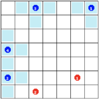
Figure 2: State visualization of benchmark environments. (a) The state of a PP-4v2 game is represented as a grid world, where blue vertices and red vertices denote predators and preys respectively. (b) The image based state for the pommerman environment.

Setup for the pommerman environment.

This environment involves four agents, and any agent can move in one of four directions, place a bomb, or do nothing. As shown in Figure 2, a state is represented as a colorful image consisted of square grids that are either empty, wooden, or rigid. An empty grid allows any agents to enter it. A wooden grid can not be entered but can be destroyed by a bomb. A rigid grid is unbreakable and impassable. When a bomb is placed in a grid, it will explode after 10 time steps. The explosion will destroy any adjacent wooden grids and kill any agents who locate around the bomb and are within 4-grids away from the bomb. If all agents of one team die, the team loses the game. The game will be terminated after $1000$ steps no matter whether there is a winner team or not. Agents get $+1$ reward if their team wins and $-1$ reward otherwise. The details of the environments are provided in Appendix. The experiments are carried out in two different games. The first one is the four agents fight against each other, denoted as Pomm-FFA. Another is a team match one where two teams, each of which has two agents, denoted as Pomm-Team.

Baselines and algorithm configuration.

Baselines.
To the best of our knowledge, this is the first work that considers the opponent modeling problem with purely local information. Because the existing works on opponent modeling all require the access to opponents’ information, they cannot work in our setting. Therefore, we compare the proposed DOMAC algorithm with one of the most popular multi-agent RL algorithms: multi-agent actor-critic (MAAC) (Lowe et al. 2017) which is the discrete version of multi-agent deep deterministic policy gradient (MADDPG). Because MAAC does not incorporate opponent modeling, it is compatible with our setting where opponents’ true information is not available. Also, we further integrate MAAC with our OMA and CDC respectively to generate another two baselines. Let OMAC denote the baseline that combines MAAC with OMA and DMAC denote the baseline that combines MAAC with CDC. The comparison with OMAC and DMAC can demonstrate the impact of OMA and CDC, and thereby justify our design. Furthermore, we consider the actual opponent policy as the ground truth to evaluate the performance of the learned imaginary opponent model. We use the actual opponent policy to sample opponent actions during training, whose performance is regarded as the upper bound (UB).

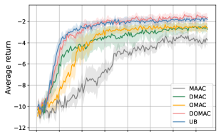
(a) Average return for PP-2v1.

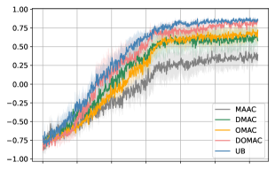
(b) Average return for Pomm-FFA.

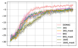
(c) Study for OMA action space in PP-4v2.

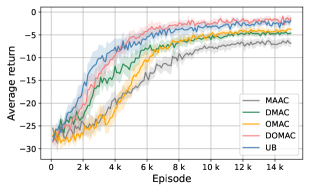
(d) Average return for PP-4v2.

(e) Average return for Pomm-Team.

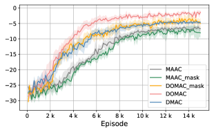
(f) Study for masked observation in PP-4v2.

Figure 3: Results of performance evaluation and ablation studies.

Algorithm configuration.

For PP-2v1 and PP-4v2, the $\rho_{\theta_{i},\psi_{i}}$ and $G_{\phi_{i}}$ of each controlled agent $i$ are both multi-layer perceptrons (MLP) with $3$ hidden layers of dimensionality $64$. We train the networks for $E=15,000$ episodes using a single environment. The parameters of the networks are updated by Adam optimizer (Kingma and Ba 2015) with learning rate for $\rho_{\theta_{i},\psi_{i}}$ and $G_{\phi_{i}}$ as $2.5e-4$ and $1e-4$. Note that rather than updating the networks for every $T_{f}$ steps as described in Algorithm 1, here we update the networks with data collected from entire $10$ episodes because the predator-prey environment consumes less memory for storing data. We set the number of quantiles as $K=5$, the discounting factor as $\gamma=0.95$, and the entropy coefficient as $\alpha_{i}=0.01$. The sample size of PP-4v2 is $l=10$. The others follow the default setting of Pytorch (Paszke et al. 2017).

The configuration for Pomm-FFA and Pomm-Team is generally the same as that of the predator-prey games. However, here $\rho_{\theta_{i},\psi_{i}}$ and $G_{\phi_{i}}$ are both convolutional neural networks (CNN) with $4$ hidden layers, each of which has $64$ filters of size $3\times 3$, as the observations are image-based. Between any two consecutive CNN layers, there is a two-layer MLP of dimension $128$. The learning rate for $\rho_{\theta_{i},\psi_{i}}$ and $G_{\phi_{i}}$ are both $2.5e-5$. We parallel $16$ environments during training and the number of forward step is $T_{f}=5$, that is, we update the networks after collecting $5$ steps of data from $16$ environments at each iteration. The total number of training episodes is $E=624,000$. We set the sample size $l$ in Pomm-FFA and Pomm-Team as 80 and 25 separately. All experiments are carried out in a machine with Intel Core i9-10940X CPU and a single Nvidia GeForce 2080Ti GPU. We will make all our data and codes public after the work is accepted.

Experiment results

Analysis of the average return.

We first compare the overall performance of DOMAC with baselines in the four games. The results are summarized in Figure 3(a), 3(d), 3(b), and 3(e). We measure the performance in terms of the approximate expected return, and each model is trained with 8 random seeds. Specifically, for PP-2v1 and PP-4v2, we evaluate all the methods with $100$ test episodes after every $100$ iterations of training, and report the mean (solid lines) and the standard deviation (shaded areas) of the average returns over eight seeds. Similarly, for Pomm-FFA and Pomm-Team, all methods are evaluated with $200$ test episodes after every $1,000$ training iterations. From the curves, we observe that the returns of DOMAC are close to the UB, and consistently outperform other three baselines with a faster convergence speed in all benchmark games while possessing a lower variance, which basically confirm that our method is an effective variant for solving the POMG without opponents’ information. In particular, including the opponent models (OMAC) can boost the performance of the actor-critic algorithm with pure centralized critic (MAAC). In addition, turning the vanilla critic (state-action value function) into distributional critic also helps to learn better policies (DMAC performs better than MAAC). These two results show that both the opponent models and the CDC have benefits for improving the performance alone.

Ablation studies for OMA and CDC.

(a) Study for trained OM.

(b) Average entropy of OM.

(c) Average KLD of OM.

Figure 4: Impacts of the distributional critic on opponent models (OM) and policies for game PP-4v2.

Throughout these ablation studies, we use game PP-4v2 as a demonstration. To investigate whether arbitrary trainable OMA can introduce improvement, we conduct an ablation study for the OMA to see how it affects the training of DOMAC, and the results over 8 random seeds are shown in Figure 3(c). We change the output dimension $d$ of opponent models to 3, 8, and 16 respectively while retaining other configurations. Note that the opponent action space size is 5. We denote these setting as “3AS”, “8AS”, and “16AS” respectively in Figure 3(c). It can see that the original DOMAC learns faster and better than the other ones. We also notice that the performance of $d=3$ and $d=8$ are consistently better than that of $d=16$ for the entire training period. It implies that the opponent model can infer more reliable information if its output dimension is close to the opponent action space size. Because the above results indicate that OMA performance is affected by the output dimension, we suspect whether it is the local observations that occasionally provide opponent information for learning. If this is the case, the opponent model whose output dimension is the same as opponent action space size can indeed better handle the received observation. To investigate this possibility, we conduct another experiment in DOMAC and MAAC where we mask out the opponent information when the agent observes the opponents and retains other configurations. The results are denoted as “DOMAC_mask” and “MAAC_mask” in Figure 3(f). It shows that when masking out the opponent information, the performance of “DOMAC_mask” is weak to “DOMAC”, which means that DOMAC indeed learns something from the observations that contain the opponent information (i.e., the observed coordinate values in our experiments). However it still outperform MAAC and “MAAC_mask”, which shows that OMA helps to make better decisions in our method.

To further verify that the imaginary opponent models truly help to learn a better policy, we perform a pair of experiments. The first one uses trained and fixed opponent models and trains the actor from scratch while the second one uses randomly initialized and fixed opponent models instead. The average returns are plotted in Figure 4(a). It is obvious that the DOMAC with trained opponent models learns faster than the one without, which indicates that the agent can infer the behaviors of its opponents and take advantage of this prior knowledge to make better decisions, especially at the beginning stage of the learning procedure. It shows that our opponent models can effectively reason about the opponents’ intentions and behaviors even with local information.

Exposing connections between OMA and CDC.
We are curious about how the centralized distributional critic (CDC) changes the way the opponent models (OM) and the policy learn. We answer this question from two perspectives. On one hand, we show that, with the help of the CDC, the opponent models are more confident in predicting opponents’ actions, and the predictions are also more accurate. On the other hand, the CDC can assist the policy in identifying actions that yield more rewards, which results in better policies. Here we also use game PP-4v2 as a demonstration. The results for the rest games are in Appendix (Figure A1).

To prove that the opponent models are more accurate in predicting opponent actions with CDC, we adopt two metrics: 1). We compute the average entropy of the probability distribution over predicted opponents’ actions, which measures the confidence of the prediction. The less average entropy is, the more certain are the agents about the predicted opponents’ actions. 2). We compute the Kullback–Leibler divergence (KLD) (Kullback and Leibler 1951) between the predicted and the ground truth opponents probability distribution. The KLD is the direct measure of the distance between the opponent models and the true opponent policies. The less the KLD is, the more similar is the modeled policy to the true one. When $\text{KLD}=0$, the opponent models exactly match the ground truth opponent policies. From Figures 4(b) and 4(c), we conclude that the CDC can increase the training speed (faster descent) and improve the reliability and confidence (lower KLD and entropy) of the opponent models. Note that for the pommerman environment, we can not access the opponents’ policies but their actions instead due to the environment restrictions. Therefore, in Pomm-FFA and Pomm-Team games, we replace KLD with cross entropy loss (Zhang and Sabuncu 2018) which has a similar effect. The second argument, i.e., the CDC helps policy to identify actions with more rewards, is supported by the results in Figure 3(f), where the performance of DMAC is better than “MAAC” and “MAAC_mask”. Note that the expected returns are still lower than DOMAC, which implies that the integration of OMA and CDC is essential for our method.

Conclusion and future work

This paper proposes a distributional opponent model aided actor-critic (DOMAC) algorithm by incorporating the distributional RL and imaginary opponent models into the actor-critic framework. In DOMAC, the imaginary opponent models receive as input the controlled agents’ local observations which realizes the opponent modeling when opponents’ information are unavailable. With the guide of the distributional critic, we manage to train the actor and opponent models effectively. Extensive experiments demonstrate that DOMAC not only obtains a higher average return but also achieves a faster convergence speed. The ablation studies and the baselines OMAC and DMAC prove that the OMA and CDC are both essential parts of our algorithm in the sense that the CDC leads to a higher-quality OMA and in turn, the better OMA helps to improve the overall performance. Based on our above analysis, the proposed integration of OMA and CDC has the potential to improve the performance of various RL algorithms. However, our work only limits its application to the on-policy multi-agent actor-critic algorithm. To address this limitation, we plan to incorporate the distributional critic and opponent modeling into other RL frameworks, e.g., value-based RL or off-policy RL.

Appendix A Distributional opponent model aided policy gradient theorem

In this part, we present the details about the distributional opponent model aided policy gradient theorem. To clarify the idea of this work, we first compare the traditional MARL algorithms with the existing works on opponent modeling. Specifically, the traditional MARL algorithms (e.g., MAAC (Lowe et al. 2017)) use the information (observations and actions) of the controlled agents to train the team policy. These algorithms normally consider the opponents as a part of the environment. In comparison, the existing works on opponent modeling use opponent models to predict the goal/actions of the opponents so that the controlled team can make better decisions given those predictions. However, these opponent modeling works need to use the true information of the opponents to train the opponent models. In this work, we don’t use the opponents’ observations and actions to train the opponent model directly because we consider the setting where the opponent’s information is inaccessible. That means our work tries to maintain the advantages brought by the opponent models while using the same information as the traditional MARL algorithms. However, this brings a challenge that we don’t have the true opponent actions to act as the training signal of our opponent model. To find an alternative training signal, we propose to use the distributional critic. Because the distributional critic can provide the training signal for the controlled agent’s actions while our controlled agent’s actions are conditioned on the outputs of opponent models, the distributional critic enable the training of opponent models without true opponent actions. In the below, we present proofs of our theorem introduced in the main text.

Proposition A.1.

In a POMG, under the opponent modeling framework defined, the gradient $\theta_{i}$ for OMA controlled agent $i$ is given as:

$$\begin{split}\nabla_{\theta_{i}}J(\theta_{i},\psi_{i})&=\mathbb{E}_{\rho_{\theta_{i},\psi_{i}}}\Bigl{[}\nabla_{\theta_{i}}\log(\rho_{\theta_{i},\psi_{i}})\cdot\\ &[\mathbb{E}(Z_{i})-\alpha_{i}\log(\rho_{\theta_{i},\psi_{i}})-\alpha_{i}]\Bigr{]}.\end{split}$$ (14)

For each opponent agent $k$, the gradient of parameters $\psi_{ik}$ is given as:

$$\begin{split}\nabla_{\psi_{ik}}J(\theta_{i},\psi_{i})&=\mathbb{E}_{\rho_{\theta_{i},\psi_{i}}}\Bigl{[}\nabla_{\psi_{ik}}\log(\rho_{\theta_{i},\psi_{i}})\cdot\\ &[\mathbb{E}(Z_{i})-\alpha_{i}\log(\rho_{\theta_{i},\psi_{i}})-\alpha_{i}]\Bigr{]},\end{split}$$ (15)

where $\rho_{\theta_{i},\psi_{i}}$ is defined in Equation (4) (in the main paper).

Proof. For notational convenience, $Z_{i}(\mathbf{o},\mathbf{a})$ can be considered as $Z_{i}$, and $\rho_{\theta_{i},\psi_{i}}(a_{i}|o_{i})$ can be simplified as $\rho_{\theta_{i},\psi_{i}}$. Then the objective in Equation (6) (in the main paper) can be written as:

$$J(\theta_{i},\psi_{i})=\sum_{a_{i}}\rho_{\theta_{i},\psi_{i}}[\mathbb{E}(Z_{i}))-\alpha_{i}\log\rho_{\theta_{i},\psi_{i}}].$$ (16)

The policy gradient of parameter $\theta_{i}$ can be calculated as:

$$\begin{split}\nabla_{\theta_{i}}J(\theta_{i},\psi_{i})&=\sum_{a_{i}}\nabla_{\theta_{i}}\rho_{\theta_{i},\psi_{i}}\mathbb{E}(Z_{i})\\ &-\alpha_{i}\sum_{a_{i}}\nabla_{\theta_{i}}[\rho_{\theta_{i},\psi_{i}}\log\rho_{\theta_{i},\psi_{i}}]\\ &=\sum_{a_{i}}\nabla_{\theta_{i}}\rho_{\theta_{i},\psi_{i}}\mathbb{E}(Z_{i})\\ &-\alpha_{i}\sum_{a_{i}}\nabla_{\theta_{i}}\rho_{\theta_{i},\psi_{i}}[\log\rho_{\theta_{i},\psi_{i}}+1]\\ &=\sum_{a_{i}}\nabla_{\theta_{i}}\rho_{\theta_{i},\psi_{i}}[\mathbb{E}(Z_{i})-\alpha_{i}\log\rho_{\theta_{i},\psi_{i}}-\alpha_{i}]\\ &=\sum_{a_{i}}\rho_{\theta_{i},\psi_{i}}\nabla_{\theta_{i}}\log\rho_{\theta_{i},\psi_{i}}[\mathbb{E}(Z_{i})\\ &-\alpha_{i}\log\rho_{\theta_{i},\psi_{i}}-\alpha_{i}]\\ &=\mathbb{E}_{\rho_{\theta_{i},\psi_{i}}}\Bigl{[}\nabla_{\theta_{i}}\log\rho_{\theta_{i},\psi_{i}}[\mathbb{E}(Z_{i})\\ &-\alpha_{i}\log\rho_{\theta_{i},\psi_{i}}-\alpha_{i}]\Bigr{]}.\end{split}$$ (17)

Since $\psi_{i}=\{\psi_{ik}\}$, then $\nabla_{\psi_{i}}J(\theta_{i},\psi_{i})=\{\nabla_{\psi_{ik}}J(\theta_{i},\psi_{i})\}$. For each opponent agent $k$, the gradient of parameter $\psi_{ik}$ can be calculated as:

$$\begin{split}\nabla_{\psi_{ik}}J(\theta_{i},\psi_{i})&=\sum_{a_{i}}\nabla_{\psi_{ik}}\rho_{\theta_{i},\psi_{i}}\mathbb{E}(Z_{i})\\ &-\alpha_{i}\sum_{a_{i}}\nabla_{\psi_{ik}}[\rho_{\theta_{i},\psi_{i}}\log\rho_{\theta_{i},\psi_{i}}].\end{split}$$ (18)

Based on the Equation (4) (in the main paper), we can conclude that the parameters of $\theta_{i}$ and ${\psi_{ik}}$ are independent. Then we can further obtain that

$$\begin{split}\nabla_{\psi_{ik}}J(\theta_{i},\psi_{i})&=\mathbb{E}_{\rho_{\theta_{i},\psi_{i}}}\Bigl{[}\nabla_{\psi_{ik}}\log\rho_{\theta_{i},\psi_{i}}[\mathbb{E}(Z_{i})\\ &-\alpha_{i}\log\rho_{\theta_{i},\psi_{i}}-\alpha_{i}]\Bigr{]}.\end{split}$$ (19)

Appendix B Concerns about POMDP setting

In this work, we apply the distributional RL to the POMDP setting. Note that most of the existing works focus on the MDP setting, i.e., they use the global states as the input of the centralized critic while we use the joint observations instead. One may have the concern about whether it is feasible to learn with the joint observations. To address this concern, we would like to first clarify what a state $s$ is. By definition, a state $s$ is one configuration of all agents and the external environment. However, in practice, a state being used by the algorithms often cannot represent the configuration of external environment completely because there are many latent variables that can affect the state transition. For example, in Atari games, a state is an image that represents the current game status while the internal random seed of the simulator can affect the future states and it cannot be obtained by the learning algorithms. Therefore, when a learning algorithm takes a state as input, the state actually means the full information that is available to the algorithm. For the latent variables that the algorithm has no access to, we use the state transition function to depict the randomness brought by them.

In this sense, when learning the critic in POMDP setting, it is equivalent to MDP setting as long as the critic takes all available information (i.e., joint observation of all controlled agents) as input. Specifically, the return expectation of MDP setting is over the trajectories resulting from the state transition function $P(s^{\prime}|s,a)$ and agent policies, i.e., $\mathbb{E}_{{s}\sim P(s^{\prime}|s,a),a\sim\pi}[\mathbb{E}(Z({s},{a}))]$. Similarly, we can let the return expectation of POMDP setting to be over the trajectories resulting from the observation transition function $P(o^{\prime}|o,a)$ and agent policies, i.e., $\mathbb{E}_{{o}\sim P(o^{\prime}|o,a),a\sim\pi}[\mathbb{E}(Z({o},{a}))]$ (Equation (5) in our paper). Based on the state transition function $P(s^{\prime}|s,a)$ and observation function $\mathcal{O}(o|s)$, we can define the observation transition function as

$$P(o^{\prime}|o,a)=\sum_{s}P(s|o)\sum_{s^{\prime}}P(s^{\prime}|s,a)\mathcal{O}(o^{\prime}|s^{\prime}),$$ (20)

where $P(s|o)=\frac{P(s,o)}{P(o)}=\frac{P(s)\mathcal{O}(o|s)}{\sum_{s}\mathcal{O}(o|s)P(s)}$ according to the Bayesian theorem. Like in MDP, the observation transition function depicts the randomness brought by all unobservable information. Therefore, the return expectation of MDP and POMDP actually have the same mathematical form and they only use different transition functions to depict the randomness from unavailable information. In both settings, we can sample the trajectories for return estimation without explicitly learning the state transition function or observation transition function. Note that the return estimation in POMDP generally has more uncertainty than the return estimation has in MDP because POMDP has more unavailable information to introduce randomness in the observation transition function. This, however, necessitates the use of distributional critic to better cope with the return estimation uncertainty.

Appendix C Environmental settings

Predator-prey: The states, observations, actions, state transition function, and reward function of each agent is formulated below by following the POMG convention.

• The states and observations. A grid world of size $x\times x$, e.g. Figure 2(a) (in the main paper) is a state of size $7\times 7$ containing four predators and two preys. The observation of agent $i$ is the coordinates of its location, its ID, and the coordinates of the prey $k$ relative to $i$ in $l\times l$ view, if observed.

• Actions space. Any agent, either predators or preys, has five actions, i.e. $[\texttt{up},\texttt{down},\texttt{left},\texttt{right},\texttt{no-op}]$ where the first four actions means the agent moves towards the corresponding direction by one step, and no-op indicates doing-nothing. All agents move within the map and can not exceed the boundary.

• State transition $\mathcal{T}$. The new state after the transition is the map with updated positions of all agents due to agents moving in the grid world. The termination condition for this task is when all preys are dead or for 100 steps.

• Rewards $\mathcal{R}$. All agents move within the map and can not exceed the boundary. Since the predators cooperate with each other, they share the team reward. The predators share a reward of 5 if two or more of them catch the prey simultaneously, while they are given a negative reward of -0.5 if only one predator catches the prey.

Pommerman:

• The states and observations. At each time step, agents get local observations within their field of view $5\times 5$, which contains information (board, position,ammo) about the map. The agent obtain the information of the Blast Strength, whether the agent can kick or not, the ID of their teammate and enemies, as well as the agent’s current blast strength and bomb life.

• Actions space. Any agent chooses from one of six actions, i.e. $[\texttt{up},\texttt{left},\texttt{right},\texttt{down},\texttt{stop},\texttt{bomb}]$. Each of the first four actions means moving towards the corresponding directions while stop means that this action is a pass, and bomb means laying a bomb.

• Rewards $\mathcal{R}$. In Pomm-Team, the game ends when both players on the same team have been destroyed. It ends when at most one agent remains alive in Pomm-FFA. The winning team is the one who has remaining members. Ties can happen when the game does not end before the max steps or if the last agents are destroyed on the same turn. Agents in the same team share a reward of 1 if the team wins the game, they are given a reward of -1 if their team loses the game or the game is a tie (no teams win). They only get 0 reward when the game is not finished.

Appendix D Evaluation results

Intuitively speaking, training the imaginary opponent model with local information seems more complicated and may need more data. To investigate whether the OMA and CDC can increase the computation complexity in our method, we provide the computational cost between different algorithms. We gather the number of floating-point operations (FLOPS) of a single inference and the number of parameters for each method. Table A1 shows the computation complexity of different algorithms. It shows that DOMAC has the comparable model volume and computational complexity as MAAC.

Table A1: Computational complexity in Pomm-Team

Algorithm	Params(M)	FLOPs(G)
MAAC	8.079	0.100
OMAC	8.085	0.101
MDAC	8.094	0.1005
DOMAC	8.100	0.1015

The number of quantiles may influence the algorithm performance, for example, using too few quantiles can lead to poor performance. To further reveal the influence of the quantiles number $K$ on learning the centralized distributional critic, we conduct another ablation study for different values of $K$. The results are shown in Figure A2(d), A2(e) and A2(f) where we can see that the performance of $K=5$ quantiles is consistently better than that of $K=3$ quantiles for the entire training period. This is aligned with the intuition that more quantiles can support more fine-grained distribution modeling. Thus, it better captures the return randomness and improves performance. However, the running time would increase as the number of quantiles becomes larger. To balance computational overhead and the performance, we set $K=5$ throughout the experiments. Finally, we also present the additional experiment results of ablation studies in Figure A1 and Figure A2. The results show that DOMAC outperforms baseline methods as well in other scenarios, which is supported by the results that DOMAC has the lowest entropy in Figure A1(a), A1(b),A1(c) and the highest average episode rewards in Figure A2(a), A2(b) and A2(c).

(a) Agent entropy for PP-2v1.

(b) Agent entropy for Pomm-FFA.

(c) Agent entropy in Pomm-Team.

(d) OM accuracy for PP-2v1.

(e) OM accuracy for Pomm-FFA.

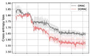
(f) OM accuracy for Pomm-Team.

(g) Entropy of OM for PP-2v1.

(h) Entropy of OM for Pomm-FFA.

(i) Entropy of OM for Pomm-Team.

Figure A1: Impacts of the distributional critic on opponent models (OM) and policies for the rest games.

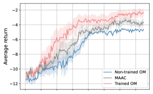
(a) Study of OM in PP-2v1.

(b) Study of OM in Pomm-FFA.

(c) Study of OM in Pomm-Team.

(d) Study for K in PP-2v1.

(e) Study for K in Pomm-FFA.

(f) Study for K in Pomm-Team.

Figure A2: Ablation studies for opponent models (OM) and quantile number $K$ in PP-2v1, Pomm-FFA, Pomm-Team.

References

- Albrecht and Stone (2017) Albrecht, S. V.; and Stone, P. 2017. Reasoning about Hypothetical Agent Behaviours and their Parameters. In Proceedings of the 16th Conference on Autonomous Agents and MultiAgent Systems, 547–555.
- Albrecht and Stone (2018) Albrecht, S. V.; and Stone, P. 2018. Autonomous agents modelling other agents: A comprehensive survey and open problems. Artificial Intelligence, 258: 66–95.
- Barth-Maron et al. (2018) Barth-Maron, G.; Hoffman, M. W.; Budden, D.; Dabney, W.; Horgan, D.; Dhruva, T.; Muldal, A.; Heess, N.; and Lillicrap, T. 2018. Distributed Distributional Deterministic Policy Gradients. In International Conference on Learning Representations.
- Bellemare, Dabney, and Munos (2017) Bellemare, M. G.; Dabney, W.; and Munos, R. 2017. A distributional perspective on reinforcement learning. In International Conference on Machine Learning, 449–458. PMLR.
- Böhmer, Kurin, and Whiteson (2020) Böhmer, W.; Kurin, V.; and Whiteson, S. 2020. Deep coordination graphs. In International Conference on Machine Learning, 980–991. PMLR.
- Brown (1951) Brown, G. W. 1951. Iterative solution of games by fictitious play. Activity analysis of production and allocation, 13(1): 374–376.
- Dabney et al. (2018a) Dabney, W.; Ostrovski, G.; Silver, D.; and Munos, R. 2018a. Implicit quantile networks for distributional reinforcement learning. In International conference on machine learning, 1096–1105. PMLR.
- Dabney et al. (2018b) Dabney, W.; Rowland, M.; Bellemare, M. G.; and Munos, R. 2018b. Distributional reinforcement learning with quantile regression. In Thirty-Second AAAI Conference on Artificial Intelligence.
- Foerster et al. (2018a) Foerster, J.; Chen, R. Y.; Al-Shedivat, M.; Whiteson, S.; Abbeel, P.; and Mordatch, I. 2018a. Learning with Opponent-Learning Awareness. In Proceedings of the 17th International Conference on Autonomous Agents and MultiAgent Systems, 122–130.
- Foerster et al. (2018b) Foerster, J.; Farquhar, G.; Afouras, T.; Nardelli, N.; and Whiteson, S. 2018b. Counterfactual multi-agent policy gradients. In Proceedings of the AAAI Conference on Artificial Intelligence, volume 32.
- He et al. (2016) He, H.; Boyd-Graber, J.; Kwok, K.; and Daumé III, H. 2016. Opponent modeling in deep reinforcement learning. In International conference on machine learning, 1804–1813. PMLR.
- Hernandez-Leal, Kartal, and Taylor (2019) Hernandez-Leal, P.; Kartal, B.; and Taylor, M. E. 2019. A survey and critique of multiagent deep reinforcement learning. Autonomous Agents and Multi-Agent Systems, 33(6): 750–797.
- Hong et al. (2018) Hong, Z.-W.; Su, S.-Y.; Shann, T.-Y.; Chang, Y.-H.; and Lee, C.-Y. 2018. A Deep Policy Inference Q-Network for Multi-Agent Systems. In Proceedings of the 17th International Conference on Autonomous Agents and MultiAgent Systems, 1388–1396.
- Hu et al. (2020) Hu, J.; Harding, S. A.; Wu, H.; Hu, S.; and Liao, S.-w. 2020. Qr-mix: Distributional value function factorisation for cooperative multi-agent reinforcement learning. arXiv preprint arXiv:2009.04197.
- Iqbal and Sha (2019) Iqbal, S.; and Sha, F. 2019. Actor-attention-critic for multi-agent reinforcement learning. In International Conference on Machine Learning, 2961–2970. PMLR.
- Kingma and Ba (2015) Kingma, D. P.; and Ba, J. 2015. Adam: A Method for Stochastic Optimization. In ICLR (Poster).
- Konda and Tsitsiklis (2000) Konda, V. R.; and Tsitsiklis, J. N. 2000. Actor-critic algorithms. In Advances in neural information processing systems, 1008–1014.
- Koul (2019) Koul, A. 2019. ma-gym: Collection of multi-agent environments based on OpenAI gym. https://github.com/koulanurag/ma-gym.
- Kullback and Leibler (1951) Kullback, S.; and Leibler, R. A. 1951. On information and sufficiency. The annals of mathematical statistics, 22(1): 79–86.
- Liu et al. (2019) Liu, M.; Zhou, M.; Zhang, W.; Zhuang, Y.; Wang, J.; Liu, W.; and Yu, Y. 2019. Multi-Agent Interactions Modeling with Correlated Policies. In International Conference on Learning Representations.
- Lowe et al. (2017) Lowe, R.; Wu, Y. I.; Tamar, A.; Harb, J.; Pieter Abbeel, O.; and Mordatch, I. 2017. Multi-agent actor-critic for mixed cooperative-competitive environments. Advances in neural information processing systems, 30.
- Lyu and Amato (2020) Lyu, X.; and Amato, C. 2020. Likelihood Quantile Networks for Coordinating Multi-Agent Reinforcement Learning. In International Conference on Autonomous Agents and Multiagent Systems (AAMAS).
- Mnih et al. (2016) Mnih, V.; Badia, A. P.; Mirza, M.; Graves, A.; Lillicrap, T.; Harley, T.; Silver, D.; and Kavukcuoglu, K. 2016. Asynchronous methods for deep reinforcement learning. In International conference on machine learning, 1928–1937. PMLR.
- Papoudakis, Christianos, and Albrecht (2021) Papoudakis, G.; Christianos, F.; and Albrecht, S. 2021. Agent Modelling under Partial Observability for Deep Reinforcement Learning. Advances in Neural Information Processing Systems, 34.
- Papoudakis, Christianos, and Albrecht (2020) Papoudakis, G.; Christianos, F.; and Albrecht, S. V. 2020. Local Information Opponent Modelling Using Variational Autoencoders. arXiv preprint arXiv:2006.09447.
- Paszke et al. (2017) Paszke, A.; Gross, S.; Chintala, S.; Chanan, G.; Yang, E.; DeVito, Z.; Lin, Z.; Desmaison, A.; Antiga, L.; and Lerer, A. 2017. Automatic differentiation in pytorch.
- Rabinowitz et al. (2018) Rabinowitz, N.; Perbet, F.; Song, F.; Zhang, C.; Eslami, S. A.; and Botvinick, M. 2018. Machine theory of mind. In International conference on machine learning, 4218–4227. PMLR.
- Raileanu et al. (2018) Raileanu, R.; Denton, E.; Szlam, A.; and Fergus, R. 2018. Modeling others using oneself in multi-agent reinforcement learning. In International conference on machine learning, 4257–4266. PMLR.
- Rashid et al. (2018) Rashid, T.; Samvelyan, M.; Schroeder, C.; Farquhar, G.; Foerster, J.; and Whiteson, S. 2018. Qmix: Monotonic value function factorisation for deep multi-agent reinforcement learning. In International Conference on Machine Learning, 4295–4304. PMLR.
- Resnick et al. (2018) Resnick, C.; Eldridge, W.; Ha, D.; Britz, D.; Foerster, J.; Togelius, J.; Cho, K.; and Bruna, J. 2018. Pommerman: A Multi-Agent Playground. CoRR, abs/1809.07124.
- Silver et al. (2014) Silver, D.; Lever, G.; Heess, N.; Degris, T.; Wierstra, D.; and Riedmiller, M. 2014. Deterministic policy gradient algorithms. In International conference on machine learning, 387–395. PMLR.
- Singh, Lee, and Chen (2020) Singh, R.; Lee, K.; and Chen, Y. 2020. Sample-based distributional policy gradient. arXiv preprint arXiv:2001.02652.
- Sutton and Barto (2018) Sutton, R. S.; and Barto, A. G. 2018. Reinforcement learning: An introduction. MIT press.
- Sutton et al. (1999) Sutton, R. S.; McAllester, D.; Singh, S.; and Mansour, Y. 1999. Policy gradient methods for reinforcement learning with function approximation. Advances in neural information processing systems, 12.
- Sutton et al. (2000) Sutton, R. S.; McAllester, D. A.; Singh, S. P.; and Mansour, Y. 2000. Policy gradient methods for reinforcement learning with function approximation. In Advances in neural information processing systems, 1057–1063.
- Tessler, Tennenholtz, and Mannor (2019) Tessler, C.; Tennenholtz, G.; and Mannor, S. 2019. Distributional policy optimization: An alternative approach for continuous control. Advances in Neural Information Processing Systems, 32: 1352–1362.
- Tian et al. (2019) Tian, Z.; Wen, Y.; Gong, Z.; Punakkath, F.; Zou, S.; and Wang, J. 2019. A regularized opponent model with maximum entropy objective. In Proceedings of the 28th International Joint Conference on Artificial Intelligence, 602–608.
- Wei et al. (2018) Wei, E.; Wicke, D.; Freelan, D.; and Luke, S. 2018. Multiagent Soft Q-Learning. In 2018 AAAI Spring Symposium Series.
- Wen et al. (2019) Wen, Y.; Yang, Y.; Luo, R.; Wang, J.; and Pan, W. 2019. Probabilistic recursive reasoning for multi-agent reinforcement learning. arXiv preprint arXiv:1901.09207.
- Yang et al. (2019) Yang, T.; Hao, J.; Meng, Z.; Zhang, C.; Zheng, Y.; and Zheng, Z. 2019. Towards Efficient Detection and Optimal Response against Sophisticated Opponents. In IJCAI.
- Yue, Wang, and Zhou (2020) Yue, Y.; Wang, Z.; and Zhou, M. 2020. Implicit distributional reinforcement learning. Advances in Neural Information Processing Systems, 33: 7135–7147.
- Zhang, Yang, and Başar (2021) Zhang, K.; Yang, Z.; and Başar, T. 2021. Multi-agent reinforcement learning: A selective overview of theories and algorithms. Handbook of Reinforcement Learning and Control, 321–384.
- Zhang and Sabuncu (2018) Zhang, Z.; and Sabuncu, M. 2018. Generalized cross entropy loss for training deep neural networks with noisy labels. Advances in neural information processing systems, 31.
- Zheng et al. (2018) Zheng, Y.; Meng, Z.; Hao, J.; Zhang, Z.; Yang, T.; and Fan, C. 2018. A deep bayesian policy reuse approach against non-stationary agents. In Proceedings of the 32nd International Conference on Neural Information Processing Systems, 962–972.
- Zintgraf et al. (2021) Zintgraf, L.; Devlin, S.; Ciosek, K.; Whiteson, S.; and Hofmann, K. 2021. Deep Interactive Bayesian Reinforcement Learning via Meta-Learning. In Proceedings of the 20th International Conference on Autonomous Agents and MultiAgent Systems, 1712–1714.