Universal Entanglement and Correlation Measure in Two-Dimensional Conformal Field Theories

Abstract

We calculate the amount of entanglement shared by two intervals in the ground state of a (1+1)-dimensional conformal field theory (CFT), quantified by an entanglement measure $\mathcal{E}$ based on the computable cross norm (CCNR) criterion. Unlike negativity or mutual information, we show that $\mathcal{E}$ has a universal expression even for two disjoint intervals, which depends only on the geometry, the central charge $c$, and the thermal partition function of the CFT. We prove this universal expression in the replica approach, where the Riemann surface for calculating $\mathcal{E}$ at each order $n$ is always a torus topologically. By analytic continuation, result of $n=\frac{1}{2}$ gives the value of $\mathcal{E}$. Furthermore, the results of other values of $n$ also yield meaningful conclusions: The $n=1$ result gives a general formula for the two-interval purity, which enables us to calculate the Rényi-$2$ $N$-partite information for $N\leq 4$ intervals; while the $n=\infty$ result bounds the correlation function of the two intervals. We verify our findings numerically in the spin-1/2 XXZ chain, whose ground state is described by the Luttinger liquid.

Introduction.— It is crucial to understand the structure of entanglement in quantum many-body systems Amico et al. (2008). For critical ground states (and the corresponding low energy sector) described by conformal field theory (CFT), people have derived rigorous results on numerous aspects of entanglement Calabrese and Cardy (2004, 2009); Fradkin and Moore (2006); Calabrese et al. (2010); Alcaraz et al. (2011); Calabrese et al. (2012); Berganza et al. (2012); Cardy and Herzog (2014); Bueno et al. (2015); Goldstein and Sela (2018), especially in one spatial dimension with an infinite number of local conformal transformations. Most notably, a single interval of length $\ell$ has a universal entanglement entropy (EE) $S=\frac{c}{3}\ln\ell$ proportional to the central charge $c$ of the CFT Calabrese and Cardy (2004, 2009).

However, for two disjoint intervals $A$ and $B$, it becomes challenging to calculate either EE of them as a whole or the classical correlation and quantum entanglement shared between $A$ and $B$. These quantities would no longer be universal while depending on the full operator content of the CFT Caraglio and Gliozzi (2008); Furukawa et al. (2009); Calabrese et al. (2009, 2011, 2012), as we briefly overview below. Since $A$ and $B$ share a mixed state, there is no unique measure that quantifies the entanglement and correlation in between Horodecki et al. (2009). Two measures have been mainly studied, namely, mutual information Furukawa et al. (2009) and positive partial transpose (PPT) negativity Calabrese et al. (2012). These quantities are calculated in the replica approach, where the Rényi version of order $n$ is expressed as a path integral on a Riemann surface composed of $n$ replicas of the system. Unlike the single-interval case, the genus of the Riemann surface grows with $n$ Calabrese et al. (2009, 2012). Since CFT calculations on high-genus surfaces become non-universal, the result for general $n$ is very complicated even for free theories Calabrese et al. (2009), which makes it difficult to analytically continue to the one-replica limit. Despite the progress that has been made Alba et al. (2010); Fagotti and Calabrese (2010); Alba et al. (2011); Rajabpour and Gliozzi (2012); Coser et al. (2014); Nobili et al. (2015); Coser et al. (2016a, b); Ruggiero et al. (2018); Grava et al. (2021); Rockwood (2022); Ares et al. (2022), there was no closed-form formula for either entanglement or correlation of two disjoint intervals in general (1+1)-d CFT ground states.

In this Letter, we solve this problem by studying the computable cross norm (CCNR) negativity as a different measure for entanglement and correlation. The advantage of this quantity is that the Riemann surface for any number of replicas always has genus $1$, which enables us to draw a connection with CFT on the torus, a much better-understood scenario than high-genus surfaces Francesco et al. (2012). By exploiting this quantity at each order $n$ and assuming the thermal free energy of the CFT is known, we derive universal formulas for not only the CCNR negativity, but also other quantifiers of entanglement and correlation in the ground state. These quantifiers include the $2$-interval purity (which generalizes the analytical result in Furukawa et al. (2009) to all CFTs), $N$-partite information for up to $N=4$ intervals, and a bound on the correlation function for two intervals. We verify our main results numerically in a spin-$1/2$ XXZ model.

For any state $\rho$ shared by two parties $A$ and $B$, define a realignment matrix $R$ with matrix elements

$$\bra{a}\bra{a^{\prime}}R\ket{b}\ket{b^{\prime}}=\bra{a}\bra{b}\rho\ket{a^{\prime}}\ket{b^{\prime}},$$ (1)

where $\left\{\ket{a}\right\}$ and $\left\{\ket{b}\right\}$ are basis for $A$ and $B$, respectively. By definition, $R$ is not necessarily a square matrix. It can be proved that $\norm{R}_{1}=\tr(\sqrt{RR^{\dagger}})\leq 1$ if $\rho$ is separable, so a state is guaranteed to be entangled if $\norm{R}_{1}>1$, so called the CCNR criterion Chen and Wu (2003). As a commonly-used mixed-state criterion, it has a similar detection capability as the PPT criterion Collins and Nechita (2016). Following the definition of PPT negativity that originates from the PPT criterion Peres (1996), the CCNR negativity is defined by

$$\mathcal{E}=\ln\norm{R}_{1},$$ (2)

as an entanglement measure. Note the similarity with the operator entanglement Rath et al. (2023); Zhou and Luitz (2017).

Now we are ready to set up the problem and present our main result for $\mathcal{E}$. For an infinite 1d system at its ground state described by a 2d CFT, we study the CCNR negativity $\mathcal{E}$ between two intervals $A=[u_{a},v_{a}]$ and $B=[u_{b},v_{b}]$, with $u_{a}<v_{a}\leq u_{b}<v_{b}$ and lengths $\ell_{\alpha}=v_{\alpha}-u_{\alpha}$ ($\alpha=a,b$). We show that $\mathcal{E}$ is related to the torus partition function $Z(\tau/2)$ of the CFT with a universal function:

$$\mathrm{e}^{\mathcal{E}}=\frac{Z\left(\tau/2\right)}{\left(\ell_{a}\ell_{b}|u_{a}-u_{b}||v_{a}-v_{b}||u_{a}-v_{b}||u_{b}-v_{a}|\right)^{c/24}},$$ (3)

where the pure imaginary modular parameter $\tau/2$ of the torus is related to the four-point ratio

$$x=\frac{(u_{a}-v_{a})(u_{b}-v_{b})}{(u_{a}-u_{b})(v_{a}-v_{b})}\in(0,1),$$ (4)

by

$$x=\left(\frac{\theta_{2}(\tau)}{\theta_{3}(\tau)}\right)^{4},$$ (5)

with $\theta_{\nu}$ being Jacobi theta functions. $Z(\tau/2)$ is the partition function of the theory on a unit circle at finite temperature $2/|\tau|$, which depends on the CFT model (see Eq. (S2) in Supplemental Material (SM) for the explicit expression). Other than this dependence, the entanglement measure $\mathcal{E}$ is completely determined by the central charge and geometry. This universality also holds for the correlation measures $Z_{n}$s that we will introduce. We note that Eq. 3 is also universal in the strong sense: different microscopic models described by the same CFT will have the same $\mathcal{E}$ in Eq. 3 (up to an additive constant).

A replica approach— Following previous works Hayden et al. (2016); Liu et al. (2022); Calabrese and Cardy (2009), $\mathcal{E}$ can be computed via a “replica trick” method (See SM for a rigorous proof):

$$\mathcal{E}=\lim_{n\rightarrow 1/2}\ln Z_{n},\quad\mathrm{where}\quad Z_{n}\equiv\tr\left[(R^{\dagger}R)^{n}\right],$$ (6)

and $\displaystyle\lim_{n\to 1/2}$ means analytic continuation from integer values of $n$ to $\frac{1}{2}$. $Z_{n}$ can be expressed as contracting $2n$ copies of $\rho$ as tensors (see Fig. 1(a) and (b)). Using imaginary time path integral, any matrix element of $\rho$ for the subsystem $A\cup B$ in the ground state equals the partition function on a 2d plane $\mathbb{C}$ with open cuts at the two intervals, as shown in Fig. 1(c). The boundary conditions at the cuts correspond to the four states $|a\rangle,|a^{\prime}\rangle,|b\rangle,|b^{\prime}\rangle$ specified by the given matrix element. Connecting the matrix elements according to Fig. 1(b), $Z_{n}$ is then the partition function on a Riemann surface $\mathcal{R}_{n}$ depicted in Fig. 1(d). The most important observation of this paper is that, as the complex plane $\mathbb{C}$ is topologically equivalent to a sphere when compactified, $\mathcal{R}_{n}$ is topologically equivalent to a torus for any value of $n$. We take the case $n=2$ as an example to shown this equivalence in Fig. 1(e). This is the key property that make the CCNR negativity easier to calculate than the PPT negativity in CFT.

When compressed to a single plane, $Z_{n}$ can be further viewed as the correlation function of some twist fields $\mathcal{T}^{\prime}_{2n}(z)$ in $2n$ copies of the original theory Cardy et al. (2008)

$$Z_{n}=\left\langle\mathcal{T}^{\prime}_{2n}(u_{a})\mathcal{T}^{\prime}_{2n}(v_{a})\widetilde{\mathcal{T}}^{\prime}_{2n}(u_{b})\widetilde{\mathcal{T}}^{\prime}_{2n}(v_{b})\right\rangle,$$ (7)

where the fields locate at the four end points of $A$ and $B$. In a nutshell, each sheet of $\mathcal{R}_{n}$ corresponds to a flavor (labeled by $1,2,\cdots,2n$) in the compressed plane, and $\mathcal{T}^{\prime}_{2n}$ and $\widetilde{\mathcal{T}}^{\prime}_{2n}$ permute the flavors by $(1\leftrightarrow 2,3\leftrightarrow 4,\cdots,2n-1\leftrightarrow 2n)$ and $(2\leftrightarrow 3,\cdots,2n\leftrightarrow 1)$ respectively. Note that these twist fields differ from $\mathcal{T}_{2n}$ for calculating EE and PPT negativity in the literature Calabrese and Cardy (2009); Calabrese et al. (2012), where the permutation is cyclic: $(1\rightarrow 2,2\rightarrow 3,\cdots,2n\rightarrow 1)$. This replica approach also works for general systems beyond 2d CFT.

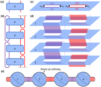
Figure 1: (a) Density matrix $\rho$ as a tensor. (b) Tensor representation of $Z_{n}$ with $n=2$, where the grey dashed lines represent the periodic boundary condition. (c) Path integral formulation for a matrix element of $\rho$, which is also a matrix element of realignment matrix $R$. (d) The Riemann surface $\mathcal{R}_{2}$ on which path integration yields $Z_{2}$. Note that sheets $1$ and $4$ are connected at the right interval $B$. (e) Smooth deformation of the surface in (d), which shows topological equivalence to a torus. The blue spheres stand for the blue sheets in (d) and the colored cylinders stand for the connections between the same area of the two neighboring sheets. The yellow dots are the points at infinity of the sheets.

Two adjacent intervals.— In 2d CFT, the Riemann surface $\mathcal{R}_{n}$ can be conformally transformed to more tractable geometries, with well-known transformation properties of primary fields such as $\mathcal{T}^{\prime}_{2n}$. As a warm-up, consider the case $v_{a}=u_{b}$ so that $A$ and $B$ are adjacent. Then $Z_{n}$ corresponds to a three-point function $Z_{n}=\left\langle\mathcal{T}^{\prime}_{2n}(u_{a})\mathcal{T}^{\otimes 2}_{n}(u_{b})\widetilde{\mathcal{T}}^{\prime}_{2n}(v_{b})\right\rangle$, where $\mathcal{T}^{\otimes 2}_{n}$, the composition of $\mathcal{T}^{\prime}_{2n}$ and $\widetilde{\mathcal{T}}^{\prime}_{2n}$, permutes the flavors by $(1\rightarrow 3,3\rightarrow 5,\cdots,2n-1\rightarrow 1)$ and $(2\rightarrow 2n,4\rightarrow 2,\cdots,2n\rightarrow 2n-2)$. This justifies the notation $\mathcal{T}^{\otimes 2}_{n}$, which means the odd and even groups of flavors factorize, and there is a cyclic permutation in each group. In CFT, three-point functions take a universal form that only depends on the geometry, the central charge $c$, and the conformal dimensions of the three operators that we compute as follows. To obtain the conformal dimension $h_{\mathcal{T}^{\prime}_{2n}}=\bar{h}_{\mathcal{T}^{\prime}_{2n}}$ for $\mathcal{T}^{\prime}_{2n}$ (the dimension for $\widetilde{\mathcal{T}}^{\prime}_{2n}$ would be the same), consider the two-point function $\left\langle\mathcal{T}^{\prime}_{2n}(u)\mathcal{T}^{\prime}_{2n}(v)\right\rangle\sim|u-v|^{-4h_{\mathcal{T}^{\prime}_{2n}}}$. The corresponding Riemann surface is $n$ independent copies of the $n=1$ case, where two sheets are connected by a cut linking $u$ to $v$, so that $\mathcal{T}^{\prime}_{2}=\mathcal{T}_{2}$. Therefore we have

$$h_{\mathcal{T}^{\prime}_{2n}}=nh_{\mathcal{T}_{2}}=n\frac{c}{24}\left(2-\frac{1}{2}\right)=\frac{n}{16}c,$$ (8)

where we use the well-known value of $h_{\mathcal{T}_{n}}$ Calabrese and Cardy (2009). Similarly, we have $h_{\mathcal{T}^{\otimes 2}_{n}}=2h_{\mathcal{T}_{n}}=\frac{c}{12}\left(n-1/n\right)$.

As a result, we find

$$Z_{n} \propto(\ell_{a}\ell_{b})^{-2h_{\mathcal{T}^{\otimes 2}_{n}}}(\ell_{a}+\ell_{b})^{2h_{\mathcal{T}^{\otimes 2}_{n}}-4h_{\mathcal{T}^{\prime}_{2n}}}$$

$$=(\ell_{a}\ell_{b})^{-\frac{c}{6}\left(n-\frac{1}{n}\right)}(\ell_{a}+\ell_{b})^{-\frac{c}{12}\left(n+\frac{2}{n}\right)}.$$ (9)

In the limit $n\rightarrow 1/2$, we get for two adjacent intervals

$$\mathcal{E}=\frac{c}{8}\left[2\ln(\ell_{a}\ell_{b})-3\ln(\ell_{a}+\ell_{b})\right]+\mathrm{const}.$$ (10)

Using standard CFT techniques, this result can be easily generalized to finite size or finite temperature Calabrese and Cardy (2009). For example, if the system is of length $L$ with periodic boundary condition, $\mathcal{E}$ at zero temperature is still given by Eq. 10, but with each length $\ell$ replaced by $\frac{L}{\pi}\sin\frac{\pi\ell}{L}$.

Two disjoint intervals.— If $A$ and $B$ are disjoint, we should use the four-point function Eq. 7, which can be rewritten as

$$Z_{n}=\left(\frac{|u_{a}-u_{b}||v_{a}-v_{b}|}{\ell_{a}\ell_{b}|u_{a}-v_{b}||u_{b}-v_{a}|}\right)^{\frac{nc}{4}}\mathcal{F}_{2n}(x)$$ (11)

using global conformal transformations and the conformal dimension in Eq. 8. Here the four-point ratio $x$ is given by Eq. 4, and the function

$$\mathcal{F}_{2n}(x)=|x(1-x)|^{\frac{nc}{4}}\left\langle\mathcal{T}^{\prime}_{2n}(0)\mathcal{T}^{\prime}_{2n}(x)\widetilde{\mathcal{T}}^{\prime}_{2n}(1)\widetilde{\mathcal{T}}^{\prime}_{2n}(\infty)\right\rangle,$$ (12)

is proportional to $Z_{n}$ defined at $(u_{a},v_{a},u_{b},v_{b})=(0,x,1,\infty)$. From now on, we focus on this particular geometry, with the operator at $\infty$ normalized by $\widetilde{\mathcal{T}}^{\prime}_{2n}(\infty)=\lim_{w\to\infty}|w|^{\frac{nc}{4}}\widetilde{\mathcal{T}}^{\prime}_{2n}(w)$. The subscript $2n$ makes $\mathcal{F}_{2}(x)$ agree with previous notations Calabrese et al. (2009, 2011, 2012), where the two-sheet Riemann surface for calculating EE or PPT negativity is exactly the same as CCNR negativity here. $\mathcal{F}_{2n}(x)$ is not universal and depends on the full operator content of the theory since the topology of the Riemann surface $\mathcal{R}_{n}$ is no longer a plane (strictly speaking, a sphere). However, the topology is just a little more complicated than a plane: it is a torus for all $n$ (see Fig. 1(d)). This special property about $\mathcal{E}$, which does not hold for EE and PPT negativity, enables us to derive universal relations between entanglement and finite temperature physics described by a torus.

We show the universal relation by first considering the simplest case $n=1$, where we introduce our main technique depicted in Fig. 2. Namely, there is a one-to-one mapping between the Riemann surface $\mathcal{R}_{1}$ and a torus $T_{\tau}$, first introduced in Dixon et al. (1987). We parametrize $\mathcal{R}_{1}$ by $w\in\mathbb{C}$ with one value of $w$ corresponding to two points in $\mathcal{R}_{1}$ (except for the four end points of $A$ and $B$). On the other hand, the torus $T_{\tau}$ is defined by the coordinate $t\in\mathbb{C}$ with periodic identifications $t\cong t+p+q\tau$, where $p$ and $q$ are integers. Here $\tau$ is the modular parameter determined by Eq. 5. Using this parametrization, the map is written as

$$w(t)=\frac{\wp(t)-e_{3}}{e_{1}-e_{3}},$$ (13)

where $\wp(t)$ is the Weierstrass elliptic function on a lattice generated by $1$ and $\tau$ , and $e_{1},e_{2},e_{3}$ equal to $\wp(1/2),\wp(\tau/2),\wp((1+\tau)/2)$ respectively with constraint

$$e_{1}+e_{2}+e_{3}=0.$$ (14)

$w(t)$ maps $T_{\tau}$ one-to-two to the complex plane, except for the four points $t=(1+\tau)/2,1/2,0,\tau/2$ that map to the four end points $w=0,1,\infty,x$ respectively, due to Eq. 5.

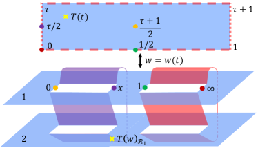
Figure 2: Schematic depiction of the one-to-one mapping in Eq. 13 between the torus $T_{\tau}$ above, represented by a rectangle with opposite sides identified, and $\mathcal{R}_{1}$ below. Points with the same color are mapped to each other.

To obtain $\mathcal{F}_{2}(x)$, we insert a stress tensor $T(w)$ in Eq. 12 and calculate the five-point function first . This is equivalent to a single-point function of the stress tensor $T(w)_{\mathcal{R}_{1}}$ on $\mathcal{R}_{1}$ with an extra prefactor $2$, since it has two sheets. According to the map in Eq. 13, this is then related to the single-point function of $T(t)$ on $T_{\tau}$ from the transformation rule

$$T(w)_{\mathcal{R}_{1}}=\left(\frac{\mathrm{d}w}{\mathrm{d}t}\right)^{-2}\left(T(t)-\frac{c}{12}\left\{w,t\right\}\right),$$ (15)

where $\left\{w,t\right\}=w^{\prime\prime\prime}/w^{\prime}-\frac{3}{2}(w^{\prime\prime}/w^{\prime})^{2}=\wp^{\prime\prime\prime}/\wp^{\prime}-\frac{3}{2}(\wp^{\prime\prime}/\wp^{\prime})^{2}$ is the Schwarzian derivative. To simplify, observe that $\wp^{\prime\prime}=\wp^{\prime}\frac{\mathrm{d}\wp^{\prime}}{\mathrm{d}\wp}=6\left(\wp^{2}+\epsilon\right)$, where $3\epsilon\equiv e_{1}e_{2}+e_{2}e_{3}+e_{3}e_{1}$, and we have used the identity

$$\wp^{\prime 2}=4\left(\wp-e_{1}\right)\left(\wp-e_{2}\right)\left(\wp-e_{3}\right),$$ (16)

together with Eq. 14. Then $\wp^{\prime\prime\prime}=12\wp\wp^{\prime}$ follows, and we get

$$\frac{1}{12}\left\{w,t\right\}=\wp(t)-\frac{9\left(\wp^{2}+\epsilon\right)^{2}}{8\left(\wp-e_{1}\right)\left(\wp-e_{2}\right)\left(\wp-e_{3}\right)},$$ (17)

for the second term in Eq. 15. For the first term, we derive its expectation in SM:

$$\left\langle T(t)\right\rangle_{T_{\tau}}=2\pi\mathrm{i}\partial_{\tau}\ln Z(\tau).$$ (18)

Taking the expectation value of Eq. 15, we obtain

$$\left\langle T(w)\mathcal{T}^{\prime}_{2}(0)\mathcal{T}^{\prime}_{2}(x)\widetilde{\mathcal{T}}^{\prime}_{2}(1)\widetilde{\mathcal{T}}^{\prime}_{2}(\infty)\right\rangle$$

$$=2\left\langle T(w)_{\mathcal{R}_{1}}\right\rangle_{\mathcal{R}_{1}}=\left(\frac{e_{1}-e_{3}}{\wp^{\prime}(t)}\right)^{2}\left(2\left\langle T(t)\right\rangle_{T_{\tau}}-\frac{c}{6}\left\{w,t\right\}\right)$$

$$=\frac{1}{w-x}\left(\frac{\left\langle T(t)\right\rangle_{T_{\tau}}}{2(e_{1}-e_{3})x(x-1)}-\frac{c}{24}\frac{2x-1}{x(x-1)}\right)+\cdots.$$ (19)

In the third line we have used Eqs. 16 and 17 and extracted the pole of order $1$ at $w=x$. According to the conformal Ward identity, the residue of the five-point function Universal Entanglement and Correlation Measure in Two-Dimensional Conformal Field Theories should equal to $\partial_{x}\left\langle\mathcal{T}^{\prime}_{2}(0)\mathcal{T}^{\prime}_{2}(x)\widetilde{\mathcal{T}}^{\prime}_{2}(1)\widetilde{\mathcal{T}}^{\prime}_{2}(\infty)\right\rangle$. Using the identity

$$2(e_{1}-e_{3})x(x-1)=-2\pi^{2}x\theta_{4}(\tau)^{4}=2\pi\mathrm{i}\frac{\mathrm{d}x}{\mathrm{d}\tau},$$ (20)

and Eq. 12, we then integrate over $x$ to get

$$\mathcal{F}_{2}(x)=Z(\tau)\left|x(1-x)\right|^{\frac{c}{6}}.$$ (21)

This establishes a universal relation between the Rényi-2 EE (or equivalently, purity) $S_{2}=-\ln Z_{1}$ of two disjoint intervals and the torus partition function. As an example, Ref. Furukawa et al. (2009) reports $\mathcal{F}_{2}(x)$ for the free compactified boson (CB) model with a critical exponent $\eta$. This is easily reproduced using Eq. 21 and the partition function Francesco et al. (2012)

$$Z_{\mathrm{CB}}(\tau)=\sqrt{\frac{\eta}{-\mathrm{i}\tau}}\frac{\theta_{3}(\eta\tau)\theta_{3}(-\eta/\tau)}{\left[\theta_{2}(\tau)\theta_{3}(\tau)\theta_{4}(\tau)\right]^{2/3}}.$$ (22)

Thanks to the torus topology, we generalize the calculation for all $n\geq 1$ in SM, where the odd (even) sheets in $\mathcal{R}_{n}$ are compressed to the up (down) sheet in Fig. 2, so that we can still use Eq. 13. We obtain our main result

$$Z_{n}=\frac{Z\left(n\tau\right)}{\left(\ell_{a}\ell_{b}|u_{a}-u_{b}||v_{a}-v_{b}||u_{a}-v_{b}||u_{b}-v_{a}|\right)^{nc/12}},$$ (23)

and Eq. 3, with simplified formulas for the two limits $x\rightarrow 0,1$ reported in SM. As Eq. 23 provides an infinite number of exact constraints on the state $\rho$, it is an interesting question what useful information beyond the CCNR negativity and purity that one can extract from the $Z_{n}$s. In SM we give a first attempt, according to the natural connection between the matrix $R$ and the correlation function $\tr\left[(\mathcal{O}_{A}\otimes\mathcal{O}_{B})\rho\right]=\bra{\mathcal{O}_{A}^{*}}R\ket{\mathcal{O}_{B}}$, where $\ket{\mathcal{O}_{A}}$ and $\ket{\mathcal{O}_{B}}$ are the vectorizations of operators $\mathcal{O}_{A}$ and $\mathcal{O}_{B}$, respectively. Thus, according to the Cauchy-Schwarz inequality, we find that $Z_{n\rightarrow\infty}$ bounds the correlation function of low-rank Hermitian operators $\mathcal{O}_{A},\mathcal{O}_{B}$ as

$$\tr\left[(\mathcal{O}_{A}\otimes\mathcal{O}_{B})\rho\right]\lesssim\lim_{n\rightarrow\infty}\ (Z_{n})^{\frac{1}{2n}}\propto(\ell_{a}\ell_{b})^{-c/8}.$$ (24)

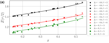
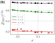
Figure 3: Predicted values using Eqs. 10 and 22 (lines) versus real values (markers) for two intervals with length $\ell_{a}=\ell_{b}=\ell$ in the ground state of the $24$-qubit XXZ chain. (a) The real values come from multiplying the numerical CCNR negativity $\mathrm{e}^{\mathcal{E}}$ of two disjoint intervals with the denominator in Eq. 3. The geometry is determined by the four-point ratio $x$ and $\ell$ indicated by the marker symbol. The three colors stand for different values of $\Delta$. (b) The real values come from Eq. 23 using the numerical $R$ matrix for different $n$ and a fixed $\Delta=-0.8$. The geometries are the same as (a). (c) CCNR negativity of two adjacent intervals, compared with the prediction Eq. 10.

Numerics.— We use the spin-$1/2$ XXZ chain with periodic boundaries

$$H=\sum_{j=1}^{L}X_{j}X_{j+1}+Y_{j}Y_{j+1}+\Delta Z_{j}Z_{j+1}$$ (25)

to test our findings, where the ground state is described by the CFT of a free compactified boson (equivalently, the Luttinger liquid) with $c=1$ and critical exponent $\eta=1-\frac{1}{\pi}\arccos\Delta$ Furukawa et al. (2009). We numerically calculate the ground state for $L=24$ sites by exact diagonalization and extract the $R$ matrix and CCNR negativity for different geometries and values of $\Delta$. As shown in Fig. 3(a) and (c), the data agrees well with our predictions Eqs. 10 and 3 using Eq. 22 for the partition function. In Fig. 3(b), the general formula Eq. 23 is also verified for $\Delta=-0.8$.

Discussion.— In conclusion, we discover that the entanglement of two disjoint intervals in ($1+1$)-d CFTs, as quantified by CCNR negativity, is universally related to the thermal partition function. Furthermore, similar relations hold for the Rényi counterparts $Z_{n}$ that provide extra information about the state $\rho$, such as the purity and a bound on correlation function. Our work thus adds to a series of rigorous findings on many-body problems Zou et al. (2021); Bertini et al. (2022); Friedman et al. (2022); Anshu et al. (2022), where it is crucial to choose the suitable entanglement measures that echo with the particular many-body structure.

We expect our results can be generalized in many directions, such as going beyond 1d ground states to excited states Alcaraz et al. (2011); Berganza et al. (2012) and finite temperature Cardy and Herzog (2014) at higher dimensions Fradkin and Moore (2006); Bueno et al. (2015). The quantity $Z_{n}$ naturally appears in the replica trick for the reflected entropy Dutta and Faulkner (2021); Akers et al. (2022, 2023), which is nicely dual to the entanglement wedge cross section Umemoto and Takayanagi (2018) in AdS/CFT. Thus it is worth exploring the meaning of Eq. 23 in holographic settings, see Milekhin et al. (2022) for a recent discussion. Since our main results can be alternatively viewed as solving four-point functions of twist fields, it is interesting to ask whether a similar structure holds for disorder operators Kadanoff and Ceva (1971); Fradkin (2017); Wang et al. (2022, 2021), the generalization of twist field operators in the symmetry perspective.

As one more generalization, one can ask about entanglement and correlation for $N>2$ intervals. Our result for the two-interval purity already yields the Rényi-2 $N$-partite information Agón et al. (2022), for $N=3$ intervals where at least two are adjacent, and $N=4$ adjacent intervals. For example, the Rényi-2 tripartite information for intervals $A,B,C$ is

$$I_{2}(A:B:C) =S_{2}(A)+S_{2}(B)+S_{2}(C)-S_{2}(AB)$$

$$\quad-S_{2}(AC)-S_{2}(BC)+S_{2}(ABC),$$ (26)

which only contains purities for one or two intervals, if $A$ is adjacent to $B$. On the other hand, for any $N$, one can construct families of Riemann surfaces that are topologically a torus, such as connecting each pair of neighboring sheets by only one interval. However, it is an open question whether our technique Eq. 13 can be generalized to such Riemann surfaces. It is also unclear whether these Riemann surfaces lead to meaningful measures of entanglement and correlation.

Acknowledgements.— We thank Andrew Lucas and Xiaoliang Qi for valuable comments. We thank Thomas Faulkner and Pratik Rath for informing us the connection to the reflected entropy. This work was supported by the National Natural Science Foundation of China Grants No. 12174216.

Supplementary Material

1 justification of the replica approach

To see Eq. 6, we write $\mathrm{e}^{\mathcal{E}}=f(1/2)$, where the function $f(\zeta)\equiv\sum_{j}\lambda_{j}^{\zeta}$ with $\lambda_{j}>0$ is the $j$th largest eigenvalue of $R^{\dagger}R$. We also have $\lambda_{j}\leq 1$ because their sum $f(1)=\tr{R^{\dagger}R}=\tr{\rho^{2}}\leq 1$. As a result, as long as $f(1/2)$ is finite, $f(\zeta)$ will be uniformly convergent, and thus analytic, in the region $\mathrm{Re}\zeta\geq 1/2$. Therefore, $f(1/2)$ can be analytically continued from the values $f(n)=Z_{n}$ when $\zeta=n$ is a positive integer.

2 expectation of the stress tensor on a torus

Consider a torus $T_{\tau}$ with modular parameter $\tau$, as shown in the upper part of Fig. 2. We calculate the expectation $\left\langle T(t)\right\rangle_{T_{\tau}}$ of the stress tensor. First, we use $t=\frac{\mathrm{i}}{2\pi}\ln z$ to map the $z$-plane to the $t$-cylinder, and get

$$\left\langle T(t)\right\rangle_{T_{\tau}}=Z(\tau)^{-1}\mathrm{tr}\left[T(t)q^{L_{0}-c/24}\bar{q}^{\bar{L}_{0}-c/24}\right],$$ (S1)

where $q=\mathrm{e}^{2\pi\mathrm{i}\tau}$, its complex conjugate $\bar{q}=\mathrm{e}^{-2\pi\mathrm{i}\bar{\tau}}$, $L_{m},\bar{L}_{m}$ are the Virasoro generators, and the partition function on $T_{\tau}$ is

$$Z(\tau)=\mathrm{tr}\left[q^{L_{0}-c/24}\bar{q}^{\bar{L}_{0}-c/24}\right].$$ (S2)

Then, the transformation $T(t)=-(2\pi)^{2}\left(\sum_{m}z^{-m}L_{m}-\frac{c}{24}\right)$ from Eq. 15 contributes to Eq. S1 only by the $L_{0}$ and $c$ terms, which yields the result Eq. 18.

3 derivation for $Z_{n>1}$

Observe that $Z_{n}$ is equivalent to the partition function on $\mathcal{R}_{1}$ with $n$ flavors on each of the two sheets: The $n$ flavors of the first (second) sheet correspond to the fields on the odd (even) sheets of $\mathcal{R}_{n}$. Denoting the field on the $j$th sheet of $\mathcal{R}_{n}$ by $\phi_{j}$, the field on the first sheet of $\mathcal{R}_{1}$ is then $\Phi_{\mathrm{o}}=(\Phi_{\mathrm{o},1},\cdots,\Phi_{\mathrm{o},n})\equiv(\phi_{1},\phi_{3},\cdots,\phi_{2n-1})$, while that on the second is $\Phi_{\mathrm{e}}=(\Phi_{\mathrm{e},1},\cdots,\Phi_{\mathrm{e},n})\equiv(\phi_{2},\phi_{4},\cdots,\phi_{2n})$. One also need to specify the continuity conditions at the two intervals that connect the two sheets of $\mathcal{R}_{1}$: The condition at $A$ is normal: $\Phi_{\mathrm{o}}=\Phi_{\mathrm{e}}$, while that at $B$ involves a cyclic permutation: $\Phi_{\mathrm{o},j}=\Phi_{\mathrm{e},j-1},(j=1,\cdots,n)$ where subscript $0\equiv n$ (see Fig. S1). As a consequence, Eq. 13 maps this theory on $\mathcal{R}_{1}$ to an $n$-component field $\Phi=(\Phi_{1},\cdots,\Phi_{n})$ living on the torus with modular parameter $\tau$, and a twisted boundary condition at the circle $\mathrm{Im}t=0$: $\Phi_{j}(t+\mathrm{i}0)=\Phi_{j-1}(t-\mathrm{i}0)$. We denote this torus by $T^{n}_{\tau,\mathrm{tw}}$ to emphasize it contains $n$ copies of the original CFT, and the boundary condition is twisted. Following the previous derivation in Universal Entanglement and Correlation Measure in Two-Dimensional Conformal Field Theories, we get

$$\left\langle T(w)\mathcal{T}^{\prime}_{2n}(0)\mathcal{T}^{\prime}_{2n}(x)\widetilde{\mathcal{T}}^{\prime}_{2n}(1)\widetilde{\mathcal{T}}^{\prime}_{2n}(\infty)\right\rangle$$

$$=\frac{1}{w-x}\left(\frac{\left\langle T(t)\right\rangle_{T^{n}_{\tau,\mathrm{tw}}}}{2(e_{1}-e_{3})x(x-1)}-\frac{nc}{24}\frac{2x-1}{x(x-1)}\right)+\cdots,$$ (S3)

where $nc$ is the central charge for $n$ copies of the original CFT. By writing down the path integral explicitly, the theory on $T^{n}_{\tau,\mathrm{tw}}$ can be unfolded as a single copy of the original CFT, on the $n$-times elongated torus $T_{n\tau}$ with no twist, as depicted in Fig. S1. Using Eq. 18, the stress tensor is then

$$\left\langle T(t)\right\rangle_{T^{n}_{\tau,\mathrm{tw}}}=n\left\langle T(t)\right\rangle_{T_{n\tau}}=2\pi\mathrm{i}\partial_{\tau}\ln Z(n\tau),$$ (S4)

Following the derivation around Eq. 20, we get

$$\mathcal{F}_{2n}(x)=Z(n\tau)\left|x(x-1)\right|^{\frac{nc}{6}}.$$ (S5)

Combining Eqs. 4, 6, 11 and S5, we arrive at Eq. 23.

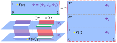
Figure S1: For $n>1$, e.g. $n=3$, Eq. 13 maps the five-point function to the torus $T^{n}_{\tau,\mathrm{tw}}$ with $n$ copies of the quantum field, and twisted boundary condition indicated by the green solid line. This is further mapped to $T_{n\tau}$ with periodic boundary conditions, with a factor $n$ in front.

4 close and far intervals limits

In the limit where $A$ and $B$ are far or close to each other with respect to their lengths, Eq. 23 (and therefore Eq. 3) reduces to a universal function independent of the function $Z(\tau)$. In the far limit, we have $x\approx 16\mathrm{e}^{\pi\mathrm{i}\tau}\to 0$ from Eq. 5. Using $L_{0},\bar{L}_{0}\geq 0$, Eq. S2 implies

$$Z(\tau^{\prime})\propto\mathrm{exp}(-\pi\mathrm{i}c\tau^{\prime}/6)\propto x^{-nc/6},$$ (S6)

where $\tau^{\prime}=n\tau\rightarrow\mathrm{i}\infty$, and Eq. 23 becomes

$$Z_{n}\propto\left(\ell_{a}\ell_{b}\right)^{-nc/4},$$ (S7)

Thus $\mathcal{E}$ approaches a constant at large separation $s=u_{b}-v_{a}$.

In the close limit $s\to 0$, we verify that Eq. 23 reduces to Universal Entanglement and Correlation Measure in Two-Dimensional Conformal Field Theories for adjacent intervals. Here $1-x\approx(\ell_{a}+\ell_{b})s/(\ell_{a}\ell_{b})\to 0$, and $\tau\to 0$ with $1-x\propto\mathrm{exp}(-\pi\mathrm{i}/\tau)$ from Eq. 5. Then from modular invariance $Z(-1/\tau^{\prime})=Z(\tau^{\prime})$ and asymptotics in Eq. S6, we have $Z(n\tau)\propto(1-x)^{-c/(6n)}$. Universal Entanglement and Correlation Measure in Two-Dimensional Conformal Field Theories is then reproduced from Eq. 23, with an extra factor $s^{-c(n+2/n)/12}$ where $s$ should be set to (some multiples of) the underlying lattice spacing.

5 $Z_{\infty}$ bounds correlation function

As shown in Fig. S2, we write

$$\quad\tr\left[(\mathcal{O}_{A}\otimes\mathcal{O}_{B})\rho\right]=\left\langle\mathcal{O}_{A}^{*}|R|\mathcal{O}_{B}\right\rangle$$

$$\leq\sqrt{\left\langle\mathcal{O}_{A}^{*}|\mathcal{O}_{A}^{*}\right\rangle\left\langle\mathcal{O}_{B}|\mathcal{O}_{B}\right\rangle}\ \norm{R}_{\infty}$$

$$=\sqrt{\tr{\mathcal{O}_{A}^{2}}\tr{\mathcal{O}_{B}^{2}}}\lim_{n\rightarrow\infty}\ (Z_{n})^{\frac{1}{2n}}$$

$$\propto\sqrt{\tr{\mathcal{O}_{A}^{2}}\tr{\mathcal{O}_{B}^{2}}}\ (\ell_{a}\ell_{b})^{-c/8}.$$ (S8)

Here in the first line, we have used (1) and defined $|\mathcal{O}_{B}\rangle=\sum_{bb^{\prime}}\left(\mathcal{O}_{B}\right)_{bb^{\prime}}|b\rangle|b^{\prime}\rangle$ and similarly for $\langle\mathcal{O}_{A}^{*}|$. The second line follows from Cauchy-Schwarz inequality, where $\norm{\cdot}_{\infty}$ is the operator norm. The third line follows by definition of the states and Eq. 6, and the last line uses Eq. S7 which holds whenever $n\tau\rightarrow\mathrm{i}\infty$. In order for the bound Section 5 to be meaningful, we require $\mathcal{O}_{A}$ (and $\mathcal{O}_{B}$) to be low-rank in the sense that $\tr{\mathcal{O}_{A}^{2}}/\norm{\mathcal{O}_{A}}^{2}_{\infty}$ grows as a sufficiently slow power law with $\ell_{a}$, so that Section 5 beats the trivial bound $\tr\left[(\mathcal{O}_{A}\otimes\mathcal{O}_{B})\rho\right]\leq\norm{\mathcal{O}_{A}}_{\infty}\norm{\mathcal{O}_{B}}_{\infty}$. For such operators, Section 5 predicts that the correlation does not depend on the separation $s$, and decays as a power law with the lengths of the two intervals, with a universal decay exponent $c/8$.

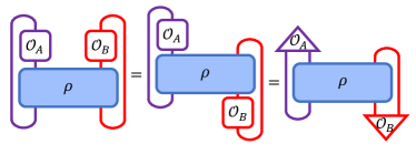
Figure S2: Relation between the $R$ matrix used in CCNR and correlation function, where operators $\mathcal{O}_{A},\mathcal{O}_{B}$ can be viewed as two vectors indicated by the triangles.

References

- Amico et al. (2008) Luigi Amico, Rosario Fazio, Andreas Osterloh, and Vlatko Vedral, “Entanglement in many-body systems,” Rev. Mod. Phys. 80, 517–576 (2008).
- Calabrese and Cardy (2004) Pasquale Calabrese and John Cardy, “Entanglement entropy and quantum field theory,” Journal of Statistical Mechanics: Theory and Experiment 2004, P06002 (2004).
- Calabrese and Cardy (2009) Pasquale Calabrese and John Cardy, “Entanglement entropy and conformal field theory,” Journal of Physics A: Mathematical and Theoretical 42, 504005 (2009).
- Fradkin and Moore (2006) Eduardo Fradkin and Joel E. Moore, “Entanglement entropy of 2d conformal quantum critical points: Hearing the shape of a quantum drum,” Phys. Rev. Lett. 97, 050404 (2006).
- Calabrese et al. (2010) Pasquale Calabrese, Massimo Campostrini, Fabian Essler, and Bernard Nienhuis, “Parity effects in the scaling of block entanglement in gapless spin chains,” Phys. Rev. Lett. 104, 095701 (2010).
- Alcaraz et al. (2011) Francisco Castilho Alcaraz, Miguel Ibáñez Berganza, and Germán Sierra, “Entanglement of low-energy excitations in conformal field theory,” Phys. Rev. Lett. 106, 201601 (2011).
- Calabrese et al. (2012) Pasquale Calabrese, John Cardy, and Erik Tonni, “Entanglement negativity in quantum field theory,” Phys. Rev. Lett. 109, 130502 (2012).
- Berganza et al. (2012) Miguel Ibáñez Berganza, Francisco Castilho Alcaraz, and Germán Sierra, “Entanglement of excited states in critical spin chains,” Journal of Statistical Mechanics: Theory and Experiment 2012, P01016 (2012).
- Cardy and Herzog (2014) John Cardy and Christopher P. Herzog, “Universal thermal corrections to single interval entanglement entropy for two dimensional conformal field theories,” Phys. Rev. Lett. 112, 171603 (2014).
- Bueno et al. (2015) Pablo Bueno, Robert C. Myers, and William Witczak-Krempa, “Universality of corner entanglement in conformal field theories,” Phys. Rev. Lett. 115, 021602 (2015).
- Goldstein and Sela (2018) Moshe Goldstein and Eran Sela, “Symmetry-resolved entanglement in many-body systems,” Phys. Rev. Lett. 120, 200602 (2018).
- Caraglio and Gliozzi (2008) Michele Caraglio and Ferdinando Gliozzi, “Entanglement entropy and twist fields,” Journal of High Energy Physics 2008, 076 (2008).
- Furukawa et al. (2009) Shunsuke Furukawa, Vincent Pasquier, and Jun’ichi Shiraishi, “Mutual information and boson radius in a critical system in one dimension,” Phys. Rev. Lett. 102, 170602 (2009).
- Calabrese et al. (2009) Pasquale Calabrese, John Cardy, and Erik Tonni, “Entanglement entropy of two disjoint intervals in conformal field theory,” Journal of Statistical Mechanics: Theory and Experiment 2009, P11001 (2009).
- Calabrese et al. (2011) Pasquale Calabrese, John Cardy, and Erik Tonni, “Entanglement entropy of two disjoint intervals in conformal field theory: II,” Journal of Statistical Mechanics: Theory and Experiment 2011, P01021 (2011).
- Horodecki et al. (2009) Ryszard Horodecki, Paweł Horodecki, Michał Horodecki, and Karol Horodecki, “Quantum entanglement,” Rev. Mod. Phys. 81, 865–942 (2009).
- Alba et al. (2010) Vincenzo Alba, Luca Tagliacozzo, and Pasquale Calabrese, “Entanglement entropy of two disjoint blocks in critical ising models,” Phys. Rev. B 81, 060411 (2010).
- Fagotti and Calabrese (2010) Maurizio Fagotti and Pasquale Calabrese, “Entanglement entropy of two disjoint blocks in xy chains,” Journal of Statistical Mechanics: Theory and Experiment 2010, P04016 (2010).
- Alba et al. (2011) Vincenzo Alba, Luca Tagliacozzo, and Pasquale Calabrese, “Entanglement entropy of two disjoint intervals in c = 1 theories,” Journal of Statistical Mechanics: Theory and Experiment 2011, P06012 (2011).
- Rajabpour and Gliozzi (2012) M A Rajabpour and F Gliozzi, “Entanglement entropy of two disjoint intervals from fusion algebra of twist fields,” Journal of Statistical Mechanics: Theory and Experiment 2012, P02016 (2012).
- Coser et al. (2014) Andrea Coser, Luca Tagliacozzo, and Erik Tonni, “On rényi entropies of disjoint intervals in conformal field theory,” Journal of Statistical Mechanics: Theory and Experiment 2014, P01008 (2014).
- Nobili et al. (2015) Cristiano De Nobili, Andrea Coser, and Erik Tonni, “Entanglement entropy and negativity of disjoint intervals in cft: some numerical extrapolations,” Journal of Statistical Mechanics: Theory and Experiment 2015, P06021 (2015).
- Coser et al. (2016a) Andrea Coser, Erik Tonni, and Pasquale Calabrese, “Towards the entanglement negativity of two disjoint intervals for a one dimensional free fermion,” Journal of Statistical Mechanics: Theory and Experiment 2016, 033116 (2016a).
- Coser et al. (2016b) Andrea Coser, Erik Tonni, and Pasquale Calabrese, “Spin structures and entanglement of two disjoint intervals in conformal field theories,” Journal of Statistical Mechanics: Theory and Experiment 2016, 053109 (2016b).
- Ruggiero et al. (2018) Paola Ruggiero, Erik Tonni, and Pasquale Calabrese, “Entanglement entropy of two disjoint intervals and the recursion formula for conformal blocks,” Journal of Statistical Mechanics: Theory and Experiment 2018, 113101 (2018).
- Grava et al. (2021) Tamara Grava, Andrew P. Kels, and Erik Tonni, “Entanglement of two disjoint intervals in conformal field theory and the 2d coulomb gas on a lattice,” Phys. Rev. Lett. 127, 141605 (2021).
- Rockwood (2022) Gavin Rockwood, “Replicated entanglement negativity for disjoint intervals in the ising conformal field theory,” Journal of Statistical Mechanics: Theory and Experiment 2022, 083105 (2022).
- Ares et al. (2022) Filiberto Ares, Pasquale Calabrese, Giuseppe Di Giulio, and Sara Murciano, “Multi-charged moments of two intervals in conformal field theory,” JHEP 09, 051 (2022), arXiv:2206.01534 [hep-th] .
- Francesco et al. (2012) P. Francesco, P. Mathieu, and D. Senechal, Conformal Field Theory, Graduate Texts in Contemporary Physics (Springer New York, 2012).
- Chen and Wu (2003) Kai Chen and Ling-An Wu, “A matrix realignment method for recognizing entanglement,” Quantum Info. Comput. 3, 193–202 (2003).
- Collins and Nechita (2016) Benoit Collins and Ion Nechita, “Random matrix techniques in quantum information theory,” Journal of Mathematical Physics 57, 015215 (2016).
- Peres (1996) Asher Peres, “Separability criterion for density matrices,” Phys. Rev. Lett. 77, 1413–1415 (1996).
- Rath et al. (2023) Aniket Rath, Vittorio Vitale, Sara Murciano, Matteo Votto, Jérôme Dubail, Richard Kueng, Cyril Branciard, Pasquale Calabrese, and Benoît Vermersch, “Entanglement barrier and its symmetry resolution: Theory and experimental observation,” PRX Quantum 4, 010318 (2023).
- Zhou and Luitz (2017) Tianci Zhou and David J. Luitz, “Operator entanglement entropy of the time evolution operator in chaotic systems,” Phys. Rev. B 95, 094206 (2017).
- Note (1) See Supplemental Material for some derivation details and additional discussions.
- Hayden et al. (2016) Patrick Hayden, Sepehr Nezami, Xiao-Liang Qi, Nathaniel Thomas, Michael Walter, and Zhao Yang, “Holographic duality from random tensor networks,” Journal of High Energy Physics 2016, 9 (2016).
- Liu et al. (2022) Zhenhuan Liu, Yifan Tang, Hao Dai, Pengyu Liu, Shu Chen, and Xiongfeng Ma, “Detecting entanglement in quantum many-body systems via permutation moments,” Phys. Rev. Lett. 129, 260501 (2022).
- Cardy et al. (2008) John L Cardy, Olalla A Castro-Alvaredo, and Benjamin Doyon, “Form factors of branch-point twist fields in quantum integrable models and entanglement entropy,” Journal of Statistical Physics 130, 129–168 (2008).
- Note (2) We refer to Francesco et al. (2012) for CFT basics used in this Letter.
- Dixon et al. (1987) Lance Dixon, Daniel Friedan, Emil Martinec, and Stephen Shenker, “The conformal field theory of orbifolds,” Nuclear Physics B 282, 13–73 (1987).
- Note (3) We refer to DLMF ; Dixon et al. (1987) for details on the special functions used in this Letter.
- Note (4) This strategy follows from the CFT calculation for EE of a single interval Calabrese and Cardy (2004, 2009).
- Zou et al. (2021) Yijian Zou, Karthik Siva, Tomohiro Soejima, Roger S. K. Mong, and Michael P. Zaletel, “Universal tripartite entanglement in one-dimensional many-body systems,” Phys. Rev. Lett. 126, 120501 (2021).
- Bertini et al. (2022) Bruno Bertini, Katja Klobas, and Tsung-Cheng Lu, “Entanglement negativity and mutual information after a quantum quench: Exact link from space-time duality,” Phys. Rev. Lett. 129, 140503 (2022).
- Friedman et al. (2022) Aaron J. Friedman, Chao Yin, Yifan Hong, and Andrew Lucas, “Locality and error correction in quantum dynamics with measurement,” (2022), arXiv:2206.09929 [quant-ph] .
- Anshu et al. (2022) Anurag Anshu, Aram W Harrow, and Mehdi Soleimanifar, “Entanglement spread area law in gapped ground states,” Nature Physics , 1–5 (2022).
- Dutta and Faulkner (2021) Souvik Dutta and Thomas Faulkner, “A canonical purification for the entanglement wedge cross-section,” JHEP 03, 178 (2021), arXiv:1905.00577 [hep-th] .
- Akers et al. (2022) Chris Akers, Thomas Faulkner, Simon Lin, and Pratik Rath, “Reflected entropy in random tensor networks,” JHEP 05, 162 (2022), arXiv:2112.09122 [hep-th] .
- Akers et al. (2023) Chris Akers, Thomas Faulkner, Simon Lin, and Pratik Rath, “Reflected entropy in random tensor networks. Part II. A topological index from canonical purification,” JHEP 01, 067 (2023), arXiv:2210.15006 [hep-th] .
- Umemoto and Takayanagi (2018) Koji Umemoto and Tadashi Takayanagi, “Entanglement of purification through holographic duality,” Nature Physics 14, 573–577 (2018).
- Milekhin et al. (2022) Alexey Milekhin, Pratik Rath, and Wayne Weng, “Computable Cross Norm in Tensor Networks and Holography,” (2022), arXiv:2212.11978 [hep-th] .
- Kadanoff and Ceva (1971) Leo P. Kadanoff and Horacio Ceva, “Determination of an operator algebra for the two-dimensional ising model,” Phys. Rev. B 3, 3918–3939 (1971).
- Fradkin (2017) Eduardo Fradkin, “Disorder Operators and their Descendants,” J. Statist. Phys. 167, 427 (2017), arXiv:1610.05780 [cond-mat.stat-mech] .
- Wang et al. (2022) Yan-Cheng Wang, Nvsen Ma, Meng Cheng, and Zi Yang Meng, “Scaling of the disorder operator at deconfined quantum criticality,” SciPost Phys. 13, 123 (2022).
- Wang et al. (2021) Yan-Cheng Wang, Meng Cheng, and Zi Yang Meng, “Scaling of the disorder operator at u(1) quantum criticality,” Phys. Rev. B 104, L081109 (2021).
- Agón et al. (2022) César A. Agón, Pablo Bueno, Oscar Lasso Andino, and Alejandro Vilar López, “Aspects of N-partite information in conformal field theories,” (2022), arXiv:2209.14311 [hep-th] .
- (57) DLMF, “NIST Digital Library of Mathematical Functions,” http://dlmf.nist.gov/, Release 1.1.7 of 2022-10-15, f. W. J. Olver, A. B. Olde Daalhuis, D. W. Lozier, B. I. Schneider, R. F. Boisvert, C. W. Clark, B. R. Miller, B. V. Saunders, H. S. Cohl, and M. A. McClain, eds.