Analyzing And Improving Neural Speaker Embeddings for ASR

Abstract

Neural speaker embeddings encode the speaker’s speech characteristics through a DNN model and are prevalent for speaker verification tasks. However, only a few inconclusive studies have investigated the usage of neural speaker embeddings for an ASR system. In this work, we present our efforts w.r.t integrating neural speaker embeddings into a Conformer-based hybrid HMM ASR system. For ASR, our improved embedding extraction pipeline in combination with the Weighted-Simple-Add integration method results in x-vector and c-vector reaching on par performance with i-vectors. We further analyze, compare and combine different speaker embeddings. We improve our already strong baseline by switching to one cycle learning schedule while reducing the training time. By further adding neural speaker embeddings, we gain additional improvements. This results in our best Conformer-based hybrid ASR system with speaker embeddings achieving 9.0% WER on Hub5’00 and Hub5’01 while only training on SWB 300h.

1 Introduction & related work

For quite some time, speaker adaptation methods have been used to build robust automatic speech recognition (ASR) systems [1], aiming at reducing the divergence of distribution caused by various speakers in the train and test datasets, compensating for differing vocal tracts, gender, accents, dialects, and further general speaker characteristics. Methodically, speaker adaptation is subdivided into different types of approaches, namely model space and feature space approaches.

Model space approaches accommodate speaker-specific representations within the acoustic model (AM) [2, 3, 4, 5, 6, 7, 8] or add additional auxiliary losses in a multitask or adversarial training fashion, while feature space approaches focus on the input to the AM. For feature space approaches, two common methods exist. Firstly, transforming the input feature vectors to be speaker normalized or speaker-dependent, for example with Vocal Tract Length Normalization [9] and Maximum Likelihood Linear Regression [10, 11]. Secondly, by augmenting the model with speaker embeddings [12, 13]. The specific integration method for a chosen speaker embedding depends on the AM architecture. Concatenating the i-vector to the network input gives performance gains for a bi-directional long-short term memory (BLSTM) recurrent neural network (RNN) AM in a hybrid modeling approach [14]. The identical integration method leads to performance degradation when utilizing a Conformer AM [15]. In our previous work [16], we proposed an integration method suited to the Conformer AM: Weighted-Simple-Add, in which we add the weighted speaker embeddings to the input of the multi-head self-attention (MHSA) module. However, this approach only works well for i-vectors but not for neural speaker embeddings, in our case x-vectors. This trend can also be observed throughout the research literature, as i-vectors are widely used for ASR [14, 16, 1, 17], but x-vectors and other neural embeddings are not. To the best of our knowledge, there has only been very limited research on neural speaker embeddings for ASR. Research on neural speaker embeddings has been focused on speaker verification and recognition. For these two tasks, neural speaker embeddings perform highly competitive. In [18, 19], (neural) speaker embeddings have been applied to different ASR systems, but no clear statement on which neural or non-neural speaker embedding to favour can be made. Besides, [18, 19] have the drawback that the models utilized are not state-of-the-art anymore, namely deep neural network (DNN) or BLSTM based. In this work, we focus on understanding the short-comings of current neural speaker embeddings for ASR. Additionally, we integrate the neural speaker embeddings into a highly competitive Conformer AM baseline. The inherently more powerful neural model compared to the Gaussian mixture model (GMM) should extract more expressive speaker embeddings. But the speaker embedding extraction is tailored to the speaker verification and recognition task, thus leading to performance degradation when applied to ASR. We investigate methods to extract speaker embeddings more suitable for the ASR task.
The main contributions of this paper are:

1. proposing an improved extraction pipeline for neural speaker embeddings, which are performant in an ASR system. The resulting x-vector and c-vector from our improved extraction pipeline improve our ASR system by $\sim$3% relative word error rate (WER) on Hub5’00.

2. improving our Switchboard baseline by using one cycle learning rate (OCLR), leading to a relative WER improvement of $\sim$3% relative and a 17% reduction in overall training time.

3. verifying the Weighted-Simple-Add method on the LibriSpeech dataset, resulting in a relative WER reduction of 5.6% on test-other.

We introduce the combination of these methods and show that neural speaker embeddings can reach the same performance as GMM-based speaker embeddings, namely i-vectors. Although the individual parts of the pipeline are not new, the application in this manner for ASR is novel. Additionally, we demonstrate a training setup in which we can achieve the same performance as i-vectors. Switching from a GMM-based speaker embedding to a neural-based one without performance degradation, opens up the possibility of integrating the speaker embedding network into the neural AM encoder, leading to joint and multi-task training strategies.

2 Speaker embeddings

Every speaker’s speech has unique characteristics due to gender, age, vocal tract variations, personal speaking style, intonation, pronunciation pattern, etc. Speaker embeddings capture these speaker characteristics from the speech signal in the form of a learnable low-dimensional fixed-size vector. The classical technique is based on a GMM-universal background model (UBM) system which extracts an i-vector [12] as a feature vector.

2.1 Neural speaker embedding

Neural speaker embeddings are extracted from the bottleneck layer of a DNN, which given speech data as input is trained in a supervised manner to discriminate between speakers. Given the strong representation capability of DNNs in learning highly abstract features, neural embeddings have outperformed i-vectors in speaker verification and speaker identification tasks [13, 20, 21]. However, when applying neural speaker embeddings as a speaker adaptation method for ASR, in general, i-vectors still outperform neural speaker embeddings [16, 19]. In this work, we propose an improved extraction pipeline for neural speaker embeddings which is more suitable for speaker adaptation in ASR tasks.

2.1.1 Neural extraction model

Choosing an appropriate neural network (NN) for the neural speaker embeddings is vital. In this work, two neural architectures are chosen: the time delay neural network (TDNN) based x-vector [13] and the Multi-scale Feature Aggregation (MFA)-Conformer based c-vector [21]. The well-known x-vector captures the speaker characteristics locally via the TDNN structures in the bottom layers. The newly proposed MFA-Conformer model captures speaker characteristics locally AND globally via a self-attention mechanism and aggregates hidden representations from multiple layers within the NN. Since the lower layers are more significant for learning speaker discriminative information [22], such multi-level aggregation can make the speaker representation more robust. Both models apply a temporal pooling layer to aggregate frame-level speaker features to obtain an utterance-level speaker embedding. This aggregation across the time dimension is crucial for extracting speaker embeddings for ASR. In this work, we compare four different temporal pooling methods within the NN: average pooling, statistics pooling [23], attention-based pooling [24], and attentive statistics pooling [25].

2.1.2 Post-processing methods

After extracting the embeddings from the NN, post-processing is applied to boost the quality of the speaker representations. We apply three standard post-processing procedures. Firstly, subtract the global mean to center the representations. Secondly, use linear discriminant analysis (LDA) to maximize the variance between the speaker embeddings of different speakers clusters and minimizes intra-speaker variance caused by channel effects [12]. Thirdly, apply length (L2) normalization to normalize the euclidean length of each embedding to unit length [19]. Besides, in order to generate embeddings on a recording- or speaker-level, we simply average the embeddings corresponding to the same recording or speaker.

2.1.3 Improved extraction pipeline

An i-vector is designed to capture the highest mode from the total variability space, and can therefore encode both speaker and channel characteristics. However, the neural speaker embedding is trained to discriminate between speakers and thus focuses on speaker-specific information. As a result, the neural speaker embeddings capture less information, which might be helpful for speaker adaptation, namely channel and other acoustic characteristics, compared to the i-vector. This information loss could be a cause of the performance degradation of neural speaker embeddings [18, 16].

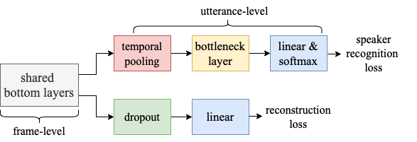
Figure 1: The speaker embedding model with auxiliary reconstruction loss.

To let the neural speaker embeddings encode additional channel and acoustic information, on the layer below the temporal pooling layer, we add an auxiliary reconstruction loss. It consists of a linear layer with dropout on the input, followed by an auxiliary mean squared error (MSE) loss to reconstruct the acoustic inputs, which can be seen in Figure 1. Suppose the layer representation is $h_{t}$ and the acoustic inputs are $x_{t}$. The reconstruction loss can be formulated as

$$\mathcal{L}=\frac{1}{2}\sum_{t=1}^{T}\sum_{c=1}^{C}(h_{t,c}-x_{t,c})^{2}$$

where C is the corresponding feature dimension. This allows us to capture additional channel and acoustic information within the speaker embedding. Overall, we propose a better extraction pipeline: 1. train speaker embedding extractor with additional reconstruction loss 2. extract speaker embeddings from bottleneck layer 3. average over recordings 4. subtract the global mean

3 Experimental setup

The experiments are conducted on Switchboard 300h [26] and LibriSpeech 960h [27] datasets. For Switchboard 300h dataset, we use Hub5’00 as the development set which consists of Switchboard (SWB) and CallHome (CH) parts. CH part is much noisier. We use Hub5’01 as test set. For LibriSpeech, we use the dev-clean and dev-other as the development set. As the test set, we use test-clean and test-other. The RETURNN [28] toolkit is used to train the acoustic models and RASR [29] toolkit is used for decoding. All our configuration files and code to reproduce our results can be found online.

3.1 Baseline

We use the same Conformer architecture and experimental setting as in our previous work [16]. However, we replace the newbob learning rate (LR) schedule with OCLR schedule [30]. OCLR can improve neural network training time without hurting performance, i.e. so-called super-convergence phenomenon. Our OCLR schedule consists of three phases, in the same manner as in [31]. Firstly, the LR linearly increases from $2e-3$ to $2e-2$ for 16 full epochs. Secondly, the LR linearly decreases from $2e-2$ to $2e-3$ for another 16 full epochs. Finally, 10 more epochs are used to further decrease the learning rate to $1e-7$. For LibriSpeech, we apply the same training recipe with two changes. First, we increase the dimension of the feed-forward module to 2048 and the attention dimension to 512 with 8 heads. Second, we extend the LR schedule to fully utilize the larger amount of training data.

We use the lattice-based version of state-level minimum Bayes risk criterion [32]. The lattices are generated using the best Conformer AM and a bigram language model (LM). A small constant learning rate of 4e-5 is used.

We use 4-gram count-based LM and long-short term memory (LSTM) LM in first pass decoding [33] and Transformer LM for lattice rescoring. For Switchboard, the LSTM and Transformer LMs have perplexity 51.3 and 48.1 on Hub5’00 respectively. For LibriSpeech, we use the official 4-gram count-based LM and a LSTM LM in first pass decoding, more details can be found in [34]. If not further specified, we use the count-based LM.

3.2 Speaker embeddings extraction

All speaker embeddings are trained on either Switchboard 300h or LibriSpeech 960h dataset. The total number of speakers is 520 or 2338, accordingly. Our i-vector extraction pipeline follows the recipe described in [14]. Empirically, we observe that 200-dim i-vectors works best for us while experimenting with 100-dim, 200-dim and 300-dim. Our x-vector TDNN system follows the same architecture described in [13]. The structure of the c-vector MFA-Conformer framework is based on [21]. We use 6 conformer blocks for the embedding extractor. The attention dimension of each MHSA module is 384 with 6 attention heads. The dimension of the feed-forward module is set to 1536. The bottleneck feature dimension is set to 512 for both embedding models. For training the neural speaker embeddings, we split the training data into a train and cross-validation set. The speaker identification is reported on a cross-validation set.

4 Results

4.1 Improved baseline

In Table 1, we present our results using different LR schedules and apply our Weighted-Simple-Add method on the Switchboard dataset. We observe that switching from newbob LR to OCLR schedule greatly enhances training effectiveness, allowing a reduction from 50 training epochs to 43, while improving WER from 10.7% to 10.4% on Hub5’00. One possible explanation of this phenomenon is that a larger learning rate helps regularize the training. We also show that integrating i-vectors using Weighted-Simple-Add outperforms basic concatenation of the i-vector to the model input and improves WER from 10.4% to 10.1% on Hub5’00. A comparison experiment using the same hyper-parameters but without i-vector integration proves that the improvement does not stem from simply training longer.

Table 1: WERs [%] of improved baseline using one cycle learning rate schedule on Switchboard 300h dataset

LR schedule	I-vec integration method	WER [%]			full epochs
		Hub5’00
		SWB	CH	Total
newbob	-	7.1	14.3	10.7	50
OCLR	-	6.8	13.9	10.4	43
+ long train	-	6.6	14.1	10.4	68
+ i-vec	append to input	6.7	13.8	10.3	68
	Weighted-Simple-Add	6.7	13.5	10.1

To show the transferability of the Weighted-Simple-Add method, we perform experiments on LibriSpeech 960h dataset, shown in Table 2. The results show around 6% relative improvement in terms of WER on all sub-sets with the 4-gram LM. However, the improvement gets smaller when we recognize with an LSTM LM.

Table 2: WERs [%] speaker adaptive training by integrating i-vectors with Weighted-Simple-Add method on LibriSpeech 960h dataset

Model	LM	dev[%]		test[%]		full epochs
		clean	other	clean	other
baseline	4-gram	2.9	6.7	3.2	7.1	15
	LSTM	2.1	4.7	2.4	5.2
+ long train	4-gram	2.8	6.6	3.0	6.9	25
+ i-vec	4-gram	2.7	6.3	3.0	6.7	25
	LSTM	2.0	4.7	2.3	5.0

4.2 Temporal pooling comparison

In order to extract speaker embeddings optimized for ASR, we study the impacts of temporal pooling in embedding extractor layer. The speaker embeddings are averaged over recordings and global mean is subtracted.

Table 3: Speaker identification accuracy [%] of speaker embeddings extractor on dev set and WERs [%] of SAT using x-vectors that are aggregated with different temporal pooling methods.

Temporal Pooling Method	SpkId Accuracy [%]	WER [%]
		Hub5’00
		SWB	CH	Total
average	93.8	6.8	14.0	10.4
statistics	89.9	6.7	14.0	10.3
attention-based	94.3	6.8	14.0	10.4
attentive statistics	90.5	6.6	13.7	10.2

Table 3 shows that the speaker identification accuracy and ASR performance, measured in WER, do not correlate highly. Both statistics pooling and attentive statistics pooling outperform average pooling and attention-based pooling respectively regarding WER, but show weaker performance for speaker identification accuracy. This indicates that including the standard deviation gives some additional useful information for ASR task.

4.3 Neural speaker embedding post processing

In Table 4, we compare methods for improving the neural speaker embeddings for ASR.

Table 4: WERs [%] of SAT using DNN-based speaker embeddings that are different in aspects of speaker recognizer model and post processing level.

Post Process. Level	Subtract mean	LDA	With reconst loss	X-vec			C-vec
				Hub5’00			Hub5’00
				SWB	CH	Total	SWB	CH	Total
utterance	no	no	no	6.9	14.1	10.5	6.7	14.1	10.4
recording				6.6	13.9	10.2	6.7	13.8	10.2
speaker				6.7	13.9	10.3	6.6	13.8	10.2
recording	yes			6.6	13.7	10.2	6.6	13.8	10.2
		yes		6.6	13.8	10.2	6.7	13.7	10.2
		no	yes	6.7	13.5	10.1	6.6	13.7	10.1

We observe that the Conformer AM only improves with recording-wise or speaker-wise embeddings. This could be due to the increased context embedded into the speaker embeddings. Furthermore, we also notice that x-vector and c-vector have similar performance. Subtracting the global mean gives no improvement to the overall Hub5’00 WER, but only minor improvement in the subsets. Applying LDA has almost no effect on performance. The weighting factor for the reconstruction loss is set to 5. With the reconstruction loss, the speaker identification accuracy of the TDNN embedding model would drop from 90.5% to 85.8%. On the contrary, the WER of SAT improves from 10.2% to 10.1% on Hub5’00.

4.4 Speaker embeddings comparison

The comparison between i-vectors and neural speaker embeddings is reported in Table 5. With our proposed extraction pipeline, the WER when integrating x-vectors is reduced by 3.8% relative, i.e., from 10.5% to 10.1%, reaching the same performance as with i-vector integration. Combining i-vectors with neural embeddings by concatenation did not show any further improvement, hinting that the different speaker embeddings contain the same information. As a control experiment, we replaced the learned speaker embeddings with Gaussian noise to verify the concern that the speaker embeddings only had an effect due to a form of noise regularization. The control experiments have the same performance as the baseline, showing that the AM utilizes the speaker embeddings in the correct way.

Table 5: WERs [%] of SAT using different types of speaker embeddings.

Speaker embedding	With reconst. loss	WER [%]
		Hub5’00			Hub 5’01
		SWB	CH	Total
none	-	6.8	13.9	10.4	10.7
Gaussian noise	-	6.7	14.1	10.4	10.6
i-vec	-	6.7	13.5	10.1	10.3
x-vec	no	6.9	14.1	10.5	10.6
	yes	6.7	13.5	10.1	10.4
c-vec	no	6.7	14.1	10.4	10.6
	yes	6.6	13.7	10.1	10.5
i-vec + x-vec	yes	6.7	13.6	10.1	10.3
i-vec + x-vec + c-vec	yes	6.6	13.6	10.1	10.3

4.5 Overall result

In Table 6, we present a highly competitive and efficient Conformer hybrid ASR system with 58M parameters and trained with 74 epochs. We outperform the well-trained Conformer transducer system [31] and our previous work [16] with fewer epochs and shorter training time. Our best Conformer ASR system does not reach the state-of-the-art results by [17]. However, two important methods applied in [17], speed perturbation and a cross-utterance LM, are not used in this work but could lead to further improvements.

Table 6: Overall WER [%] comparison with literature.

Work	ASR Arch.	AM	LM	seq disc	ivec	num param	full epochs	WER [%]
								Hub
								5’00	5’01
[31]	RNNT	Conf.	Trafo	yes	no	75	86	9.2	9.3
[17]	LAS	Conf.	Trafo	no	yes	68	250	8.4	8.5
[35]	Hybrid	TDNN	RNN	yes	yes	19	-	10.4	-
[16]		Conf.	Trafo	yes	yes	58	90	9.2	9.3
ours			4-gr	no	no		43	10.4	10.7
					yes		68	10.1	10.3
				yes			74	10.0	10.1
			LSTM					9.2	9.3
			Trafo					9.0	9.0

5 Conclusion

In this work, we focus our research on neural speaker embeddings for ASR. We begin our investigations by improving our strong baseline on the Switchboard dataset with the utilization of an OCLR schedule. We apply the Weighted-Simple-Add method on top of our Switchboard baseline and confirm the method on the LibriSpeech dataset. Focusing on the shortcomings of neural speaker embeddings compared to the conventional i-vectors, we propose an improved extraction pipeline. Different design choices for the neural speaker embedding extraction pipeline are presented and compared. With our proposed pipeline, the integration of x-vector or c-vector improves the ASR system performance by $\sim$3% relative, reaching on-par performance with i-vectors. We think a more sophisticated reconstruction loss that captures the relevant information in the speaker embedding more accurately could push the performance of the neural speaker embedding ASR system beyond the ASR system with i-vectors. Moreover, we tried to combine the i-vector with neural speaker embeddings but gained no further improvement. This indicates that the neural speaker embeddings contain at least very similar information as the i-vectors. The competitive performance of the neural speaker embeddings opens up possibilities for joint training and integrating neural speaker embeddings into the AM. Overall, we present a highly competitive and efficient Conformer hybrid ASR system, approaching the state-of-the-art results but with a much smaller model and less training time.

6 Acknowledgements

This work was partially supported by a Google Focused Award. The work reflects only the authors’ views and none of the funding parties is responsible for any use that may be made of the information it contains.

References

- [1] G. Saon, H. Soltau, D. Nahamoo, and M. Picheny, “Speaker adaptation of neural network acoustic models using i-vectors,” in Proc. IEEE ASRU, (Olomouc, Czech Republic), pp. 55–59, Dec. 2013.
- [2] H. Liao, “Speaker adaptation of context dependent deep neural networks,” in Proc. IEEE ICASSP, (Vancouver, Canada), pp. 7947–7951, May 2013.
- [3] D. Yu, K. Yao, H. Su, G. Li, and F. Seide, “Kl-divergence regularized deep neural network adaptation for improved large vocabulary speech recognition,” in Proc. IEEE ICASSP, (Vancouver, Canada), pp. 7893–7897, May 2013.
- [4] F. Seide, G. Li, X. Chen, and D. Yu, “Feature engineering in context-dependent deep neural networks for conversational speech transcription,” in Proc. IEEE ASRU, (Waikoloa, HI, USA), pp. 24–29, IEEE, Apr. 2011.
- [5] P. Swietojanski and S. Renals, “Learning hidden unit contributions for unsupervised speaker adaptation of neural network acoustic models,” in Proc. IEEE Spoken Language Technology Workshop (SLT), pp. 171–176, 2014.
- [6] P. Swietojanski, J. Li, and S. Renals, “Learning hidden unit contributions for unsupervised acoustic model adaptation,” IEEE ACM Trans. Audio Speech Lang. Process., vol. 24, no. 8, pp. 1450–1463, 2016.
- [7] R. Gemello, F. Mana, S. Scanzio, P. Laface, and R. De Mori, “Adaptation of hybrid ann/hmm models using linear hidden transformations and conservative training,” in Proc. IEEE ICASSP, (Toulouse, France), pp. 1189–1192, IEEE, May 2006.
- [8] L. Bo and S. Khe Chai, “Comparison of discriminative input and output transformations for speaker adaptation in the hybrid nn/hmm systems,” in Eleventh Annual Conference of the International Speech Communication Association, (Makuhari, Chiba, Japan), 2010.
- [9] L. Welling, S. Kanthak, and H. Ney, “Improved methods for vocal tract normalization,” in Proc. IEEE ICASSP, vol. 2, (Phoenix, AZ, USA), pp. 761–764 vol.2, Mar. 1999.
- [10] C. Leggetter and P. Woodland, “Maximum Likelihood Linear Regression for Speaker Adaptation of Continuous Density Hidden Markov Models,” Computer Speech & Language, vol. 9, no. 2, pp. 171–185, 1995.
- [11] S. H. Ghalehjegh and R. C. Rose, “Regularized constrained maximum likelihood linear regression for speech recognition,” in Proc. IEEE ICASSP, pp. 6319–6323, May 2014.
- [12] N. Dehak, P. J. Kenny, R. Dehak, P. Dumouchel, and P. Ouellet, “Front-end factor analysis for speaker verification,” IEEE Transactions on Audio, Speech, and Language Processing, vol. 19, no. 4, pp. 788–798, 2011.
- [13] D. Snyder, D. Garcia-Romero, G. Sell, D. Povey, and S. Khudanpur, “X-Vectors: Robust DNN Embeddings for Speaker Recognition,” in Proc. IEEE ICASSP, (Calgary, Canada), pp. 5329–5333, Apr. 2018.
- [14] M. Kitza, P. Golik, R. Schlüter, and H. Ney, “Cumulative Adaptation for BLSTM Acoustic Models,” in INTERSPEECH, (Graz, Austria), pp. 754–758, sep 2019.
- [15] J. Deng, X. Xie, T. Wang, M. Cui, B. Xue, Z. Jin, G. Li, S. Hu, and X. Liu, “Confidence score based speaker adaptation of conformer speech recognition systems,” IEEE/ACM Transactions on Audio, Speech, and Language Processing, pp. 1–15, 2023.
- [16] M. Zeineldeen, J. Xu, C. Lüscher, R. Schlüter, and H. Ney, “Improving the training recipe for a robust conformer-based hybrid model,” in Proc. Interspeech, (Incheon, Korea), pp. 1036–1040, Sept. 2022.
- [17] Z. Tüske, G. Saon, and B. Kingsbury, “On the limit of english conversational speech recognition,” in Interspeech, (Brno, Czech), pp. 2062–2066, Sept. 2021.
- [18] J. Rownicka, P. Bell, and S. Renals, “Embeddings for dnn speaker adaptive training,” in Proc. IEEE ASRU, (Sentosa, Singapore), pp. 479–486, Dec. 2019.
- [19] A. Rouhe, T. Kaseva, and M. Kurimo, “Speaker-aware Training of Attention-based End-to-end Speech Recognition Using Neural Speaker Embeddings,” in Proc. IEEE ICASSP, (Barcelona, Spain), pp. 7064–7068, May 2020.
- [20] J. Jung, H. Heo, J. Kim, H. Shim, and H. Yu, “Rawnet: Advanced end-to-end deep neural network using raw waveforms for text-independent speaker verification,” in Proc. Interspeech, (Graz, Austria), pp. 1268–1272, Sept. 2019.
- [21] Y. Zhang, Z. Lv, H. Wu, S. Zhang, P. Hu, Z. Wu, H. Lee, and H. Meng, “MFA-Conformer: Multi-scale Feature Aggregation Conformer for Automatic Speaker Verification,” in Proc. Interspeech 2022, pp. 306–310, 2022.
- [22] Y. Tang, G. Ding, J. Huang, X. He, and B. Zhou, “Deep speaker embedding learning with multi-level pooling for text-independent speaker verification,” in Proc. IEEE ICASSP, pp. 6116–6120, IEEE, 2019.
- [23] D. Snyder, D. Garcia-Romero, D. Povey, and S. Khudanpur, “Deep neural network embeddings for text-independent speaker verification,” in Proc. Interspeech, (Stockholm, Sweden), pp. 999–1003, Aug. 2017.
- [24] F. R. Rahman Chowdhury, Q. Wang, I. L. Moreno, and L. W., “Attention-based models for text-dependent speaker verification,” in Proc. IEEE ICASSP, (Calgary, Alberta), pp. 5359–5363, Apr. 2018.
- [25] K. Okabe, T. Koshinaka, and K. Shinoda, “Attentive Statistics Pooling for Deep Speaker Embedding,” in Proc. Interspeech, (Hyderabad, India), pp. 2252–2256, Sept. 2018.
- [26] J. Godfrey, E. Holliman, and J. McDaniel, “Switchboard: Telephone Speech Corpus for Research and Development,” in Proc. IEEE ICASSP, vol. 1, (San Francisco,USA), pp. 517–520, Mar. 1992.
- [27] V. Panayotov, G. Chen, D. Povey, and S. Khudanpur, “LibriSpeech: An ASR Corpus Based on Public Domain Audio Books,” in Proc. IEEE ICASSP, (South Brisbane, Australia), pp. 5206–5210, Apr. 2015.
- [28] A. Zeyer, T. Alkhouli, and H. Ney, “RETURNN as a generic flexible neural toolkit with application to translation and speech recognition,” in Proc. of the Joint Conf. of the 47th Annual Meeting of the ACL and the 4th Int. Joint Conf. on Natural Language Processing of the AFNLP, (Melbourne, Australia), July 2018.
- [29] S. Wiesler, A. Richard, P. Golik, R. Schlüter, and H. Ney, “RASR/NN: The RWTH neural network toolkit for speech recognition,” in Proc. IEEE ICASSP, (Toronto, Canada), pp. 3281–3285, June 2014.
- [30] L. N. Smith and T. Nicholay, “Super-convergence: Very fast training of neural networks using large learning rates,” in Artificial intelligence and machine learning for multi-domain operations applications, International Society for Optics and Photonics, 2019.
- [31] W. Zhou, W. Michel, R. Schlüter, and H. Ney, “Efficient training of neural transducer for speech recognition,” in Proc. Interspeech, (Incheon, Korea), pp. 2058–2062, Sept. 2022.
- [32] M. Gibson and T. Hain, “Hypothesis Spaces for Minimum Bayes Risk Training in Large Vocabulary Speech Recognition,” in Proc. Interspeech, (Pittsburgh, USA), pp. 2406–2409, Sept. 2006.
- [33] E. Beck, W. Zhou, R. Schlüter, and H. Ney, “LSTM Language Models for LVCSR in First-Pass Decoding and Lattice-Rescoring,” ArXiv, vol. abs/1907.01030, 2019.
- [34] C. Lüscher, E. Beck, K. Irie, M. Kitza, W. Michel, A. Zeyer, R. Schlüter, and H. Ney, “RWTH ASR Systems for LibriSpeech: Hybrid vs Attention,” in Proc. Interspeech, (Graz, Austria), pp. 231–235, Sept. 2019.
- [35] S. Hu, X. Xie, S. Liu, J. Yu, Z. Ye, M. Geng, X. Liu, and H. Meng, “Bayesian learning of lf-mmi trained time delay neural networks for speech recognition,” IEEE/ACM Transactions on Audio, Speech, and Language Processing, vol. 29, pp. 1514–1529, 2021.