Collision-free Source Seeking and Flocking Control of Multi-agents with Connectivity Preservation

Abstract

We present a distributed source-seeking and flocking control method for networked multi-agent systems with non-holonomic constraints. Based solely on identical on-board sensor systems, which measure the source local field, the group objective is attained by appointing a leader agent to seek the source while the remaining follower agents form a cohesive flocking with their neighbors using a distributed flocking control law in a connectivity-preserved undirected network. To guarantee the safe separation and group motion for all agents and to solve the conflicts with the ”cohesion” flocking rule of Reynolds, the distributed control algorithm is solved individually through quadratic-programming optimization problem with constraints, which guarantees the inter-agent collision avoidance and connectivity preservation. Stability analysis of the closed-loop system is presented and the efficacy of the methods is shown in simulation results.

I Introduction

The coordination control of networked multi-agent systems pertains to the development of distributed control protocols with limited local interactions among neighboring agents such that the coordinated objectives can be realized (e.g., flocking, rendezvous, formation and consensus [1, 2]). As a family of distributed control problems, flocking is a typical form of collective motion behavior that can be found in nature and it has been studied and adopted in various disciplines including computer science [3], physics [4, 5], biology [6, 7] and robotics[1, 8]. Given the widely accepted flocking rules (cohesion, alignment, and separation), flocking is considered to be a motion synchronization or consensus problem where all the agents reach an agreement [9] and achieve a group control objective [10] in a dynamically changing environment [11, 12, 5, 13].

In practice, the agents face a trade-off between achieving flocking and keeping a safe distance from each other. The potential function method is widely implemented with the structures of leader-follower [14, 10] and virtual leader[15], where the safe separation among agents relies on the repulsive force while the attractive force contributes to the flocking cohesion [16, 17]. The dynamic programming method is presented in [18] to allow the computation of control input with the constraints of pose synchronization and collision avoidance. Recently, learning-based methods have been investigated to solve these flocking challenges where a control policy is learned via reinforcement learning [19] and Q-learning [20]. In addition to this trade-off, the networked multi-agent systems have to deal with a dynamic communication graph due to the limited sensing range that each agent has at disposal for obtaining local information in its surrounding. The graph connectivity is therefore required to be maintained to realize cohesion, and to avoid agent splitting and fragmentation [11, 12, 13, 21]. Various algebraic connectivity algorithms have been proposed in the literature where, in general, the global connectivity is maintained by maximizing the second smallest eigenvalue of the graph Laplacian [22, 23, 24].

Even though the distributed flocking control problem is well-studied for point-mass agents described by single-integrator [12, 13, 21, 15, 14] or by double-integrator [17, 18, 16, 19, 20, 25], the distributed control algorithms can not be directly implemented on unicycle agents where both the agent’s orientation and velocity need to be controlled under non-holonomic constraints. This restriction also raises difficulties in the application of control barrier functions (CBF)-based optimization of multi-agent systems, where the angular velocity will not have an effect on the time derivative of CBF and result in a mixed relative degree problem.

In this paper, we propose a constraint-driven distributed control law for source-seeking and flocking cohesion of the multi-unicycle system in an environment where an unknown source with maximum signal strength exists. Our proposed methods use only local measurements for achieving all aforementioned coordination tasks (source-seeking, flocking, collision avoidance and connectivity preservation). Our main contributions are summarized as follows.

1. (Source-signal-guided flocking) The source-signal-based flocking objective is to reach a consensus agreement where each follower maintains a desired relative source signal gradient difference with respect to its neighbors’ average. The flocking control relies on the individual source signal gradient measurement on each agent instead of the relative distance/position between each pair of connected agents as commonly used in literature. This is motivated by the chemotaxis motion of bacteria that has been adopted for the control of molecular/microrobots [26]. We assume that each agent has a local reference frame located in its mass center and shares the same orientation of North and East, such that the locally measured source signal gradient vector can be converted into this frame. Only connected agents exchange the local source measurement with each other, which implies that the leader’s state will not be shared with all followers and vice versa (i.e. it’s not an all-to-all structure).

2. (Flocking control of unicycle with nonholonomic constraint) Two types of flocking cohesion forms and the corresponding control laws are proposed for the multi-unicycle system, and the group flocking behavior can be achieved with any randomly selected initial states in the connected undirected graph.

3. (CBF with uniform relative degree) A CBF-based distributed optimization method is introduced to guarantee the topology connectivity and avoid the inter-agent collisions of the multi-agent system. A new construction of CBF is proposed with extended space for a nonholonomic multi-unicycle system to obtain a uniform relative degree. Compared to the general solutions that only constrain angular velocity for the safe motion, the proposed design provides safety/connectivity constraints on both control inputs and does not have the problem of confined control performance.

The structure of the paper is as follows. The problem formulation and notations are stated in Section II. We review the background of the source-seeking control algorithm and analyze the flocking control design in Section III. The connectivity preservation and inter-agent safety are disscussed in Section IV. The efficacy of the proposed algorithm with extensive simulation results is presented in Section V. Finally, in Section VI, we present the summary and discussion of the work.

II Preliminaries and Problem Formulation

In this section, we provide the relevant background and formulate our inter-agent collision-free source-seeking (leader) and flocking control (followers) problem. We first present the unicycle model and the flocking topology of the multi-agent system, and then introduce the control barrier function and its application for maintaining the the safety of systems.

II-A Multi-unicycle system

In this paper, we consider an unknown source $(x^{*},y^{*})$ located in the 2D plane that transmits a 2D field distribution satisfying the following assumption.

Assumption II.1.

The source field function $J(x,y)$ is a twice-differentiable, radially unbounded strictly concave function whose maximum coincides with the unknown source location $(x^{*},y^{*})$.

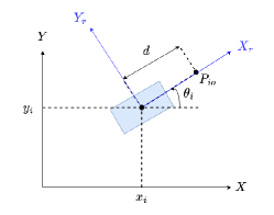
Figure 1: Unicycle model in 2D plane.

Consider a group of $n$ unicycle agents that are initialized randomly in this 2D field distribution, and they are all equipped with sensor systems that can measure the local field gradient. For each agent $i\in\{1,2,...n\}$, its kinematic dynamics is described by

$$\begin{bmatrix}\dot{x}_{i}\\ \dot{y}_{i}\\ \dot{\theta}_{i}\end{bmatrix}=\begin{bmatrix}v_{i}\cos(\theta_{i})\\ v_{i}\sin(\theta_{i})\\ \omega_{i}\end{bmatrix},$$ (1)

where $(x_{i}(t),y_{i}(t))$ denotes the position of agent $i$ in the Cartesian coordinate system and $\theta_{i}(t)$ is the heading angle with respect to the $X$-axis of the global frame of reference as illustrated in Figure 1.

We consider the following agent assignment setup. Within the group of unicycle robots, a random agent should be first assigned as the leader and maintain the role afterward. The leader’s main goal is to traverse across the field, to search and to approach the source as soon as possible, using only its own local sensor systems. The rest of the robots are assigned as the followers whose task is to form a flock with their neighbors’ signal average based on the relative source signal strength.

II-B Flocking Topology

All agents in the group are assumed to form a communication graph, including the leader and followers. The communication topology among the agents is modeled as an undirected graph $\mathcal{G}=(\mathcal{E},\mathcal{V})$ where $\mathcal{V}=\left\{1,2,...,{n}\right\}$ is the vertex set and $\mathcal{E}\subseteq\left\{(i,j):i\in\mathcal{V},j\in\mathcal{N}_{i}\right\}$ is the edge set. The set of neighbors for agent $i$ is denoted as $\mathcal{N}_{i}$, which contains all neighbors that agent $i$ can sense and communicate with. We consider an undirected graph $\mathcal{G}$ in this work, i.e., $(i,j)\in\mathcal{E}\Leftrightarrow(j,i)\in\mathcal{E}$ holds, and its adjacency matrix $A=\left[a_{ij}\right]$ is symmetric with nonzero elements $a_{ij}=1$ for $(j,i)\in\mathcal{E}$, else $a_{ij}=0$. Each agent $i$ is able to share its local sensed source signal gradient with its neighbor agents $j\in\mathcal{N}_{i}$ and aims to maintain a desired gradient error norm $d^{*}_{\nabla\bm{J}}\in\mathbb{R}_{+}$ with the neighbors’ source gradient centroid.

Once the leader agent $L$ is assigned at the initial time instant, it will maintain this role throughout the time. Accordingly, the followers set is denoted by $\mathcal{V}_{f}:=\mathcal{V}\setminus L$. Note the leader’s motion is independent of that of the followers, but it can be considered a neighboring agent if it belongs to the neighbor set $\mathcal{N}_{i}$ of the follower agent $i\in\mathcal{V}_{f}$. The communication only happens between the connected nodes, hereby the leader’s information is solely available to its neighboring followers, and the communication topology is not an all-to-all form.

II-C Control Barrier Function

Given the kinematic model of the unicycle in (1), the dynamics of each agent $i$ can be rewritten in the form of a nonlinear affine control system

$$\dot{\bm{\xi}_{i}}=f_{i}(\bm{\xi}_{i})+g_{i}(\bm{\xi}_{i})\bm{u}_{i}$$ (2)

where the state $\bm{\xi}_{i}\in\mathbb{R}^{q}$ for the unicycle agent will be further discussed in Section IV, and $f_{i}(\bm{\xi}_{i}):\mathbb{R}^{q}\rightarrow\mathbb{R}^{q},g_{i}(\bm{\xi}_{i}):\mathbb{R}^{q}\rightarrow\mathbb{R}^{q\times m}$ are locally Lipschitz continuous in $\bm{\xi}_{i}$, and the control input $\bm{u}_{i}\in\mathcal{U}_{\text{adm}}\subset\mathbb{R}^{m}$ is constrained in the set of admissible inputs. For a given continuously differentiable function $h(\bm{\xi}_{i}):\mathbb{R}^{q}\rightarrow\mathbb{R}$, we define the following three sets, which will be used throughout the paper for studying systems’ safety:

$$\mathcal{S}_{h} =\left\{\bm{\xi}_{i}\in\mathbb{R}^{q}:h(\bm{\xi}_{i})\geq 0\right\}$$ (3)

$$\partial\mathcal{S}_{h} =\left\{\bm{\xi}_{i}\in\mathbb{R}^{q}:h(\bm{\xi}_{i})=0\right\}$$ (4)

$$\text{Int}(\mathcal{S}_{h}) =\left\{\bm{\xi}_{i}\in\mathbb{R}^{q}:h(\bm{\xi}_{i})>0\right\}.$$ (5)

Whenever it is clear from the context, we omit the dependence on $h$ in these notations.

Definition II.1.

(Control barrier function) Given a set $\mathcal{S}$ defined in (3)-(5), $h(\bm{\xi}_{i})$ is a Control Barrier Function (CBF) for system (2) if there exists a class $\mathcal{K}_{\infty}$ function $\alpha$ such that

$$\sup_{\bm{u}_{i}\in\mathbb{R}^{m}}[L_{f_{i}}h(\bm{\xi}_{i})+L_{g_{i}}h(\bm{\xi}_{i})\bm{u}_{i}+\alpha(h(\bm{\xi}_{i}))]\geq 0,\quad\forall\bm{\xi}_{i}\in\mathcal{S}.$$ (6)

where $L_{f_{i}}$, $L_{g_{i}}$ denote the Lie derivatives along $f_{i}$ and $g_{i}$, respectively.

Given the CBF $h$ satisfying (6), for all $\bm{\xi}_{i}\in\mathcal{S}$, we define the set

$$K(\bm{\xi}_{i})=\left\{\bm{u}_{i}:L_{f_{i}}h(\bm{\xi}_{i})+L_{g_{i}}h(\bm{\xi}_{i})\bm{u}_{i}+\alpha(h(\bm{\xi}_{i}))\geq 0\right\}.$$ (7)

Then for any locally Lipschitz function $\bm{k}:{\mathbb{R}}^{q}\to{\mathbb{R}}^{m}$ such that $\bm{k}(\bm{\xi}_{i})\in K(\bm{\xi}_{i})$, the set $\mathcal{S}$ is forward invariant with respect to the closed-loop system (2) with $\bm{u}_{i}=\bm{k}_{i}(\bm{\xi}_{i})$, i.e. for all $\bm{\xi}_{i}(t_{0})\in\mathcal{S}$, the solution $\bm{\xi}_{i}(t)\in\mathcal{S}$ for all $t\geq t_{0}$. We refer interested readers to the related discussion in [27].

II-D Problem Formulation

As discussed in the Introduction, with the 2D field $J$ satisfying Assumption II.1, the control objective of the leader robot is to safely search the source’s location based only on its local field measurement. At the same time, the followers in the group must avoid all potential inter-agent collisions and realize a flocking by maintaining a desired gradient error norm $d^{*}_{\nabla\bm{J}}\in\mathbb{R}_{+}$ with its neighbors’ centroid. In this setup, the leader can be randomly assigned but it should maintain its role throughout. Therefore, the group source-seeking objective can be achieved by guaranteeing topology connectedness at all time. In summary, the setup of the multi-agent system is as follows.

1. All agents can measure locally the source field gradient and communicate its local information only with their neighbors. None of them has access to global information (e.g., source position or global 2D field).

2. Once the leader agent is assigned, its main task is to seek the source using the local field gradient measurement. The leader agent will only communicate its local information to its connected neighbors and not to the rest of the followers. In this setup, the followers do not know the identity of the leader as it is regarded only as a neighbor of a subset of followers.

Based on the above setup, we formulate the distributed control design problem as follows.

Inter-agent collision-free source seeking (leader) and flocking control (followers) problem: Consider a group of $n$ unicycle robots (1) traversing across a $2$D field $J$ satisfying Assumption II.1 and given a safe set $\mathcal{S}\subset\mathbb{R}^{q}$ for the extended system in (2), design a distributed control law $\bm{u}_{i}$ for each follower agent $i\in\mathcal{V}_{f}$, and a control policy for the leader $L$ such that the following motion tasks can be achieved.

1. Source seeking task: The leader robot converges to the source location $(x^{*},y^{*})$, i.e.,

   $$\lim_{t\to\infty}\left\|\left[\begin{matrix}x_{L}(t)-x^{*}\\ y_{L}(t)-y^{*}\end{matrix}\right]\right\|=0,$$ (8)

   where $(x_{L},y_{L})$ is the position of the leader.

2. Flocking cohesion and connectivity preservation task: Based on the flocking center of each follower agent $i\in\mathcal{V}_{f}$ defined by the mean of all its neighboring agents’ field gradient (i.e., $\frac{1}{{N}_{i}}\sum_{j\in\mathcal{N}_{i}}\nabla\bm{J}_{j}$), the flocking cohesion task for each follower is to converge and maintain a desired distance (i.e., $d^{*}_{\nabla\bm{J}}$) with respect to its flocking center.

   In the meantime, the connectivity of communication topology $\mathcal{G}(t)$ is preserved all the time $t\geq t_{0}$, such that no group splitting or group fragmentation is allowed.

3. Safe flocking separation and inter-agent collision avoidance task: The multi-agent system is safe at all time, i.e.,

   $${\bm{\xi}_{i}(t)\in\mathcal{S}\qquad\forall t\geq t_{0},}$$ (9)

   such that there is no collision between agents during the motion and flocking.

III Flocking Control Design

In this section, we present two distributed flocking controllers for the follower unicycle-model agents. The first one is designed based on a scalar flocking error where an offset needs to be assigned along the axis of the agent to tackle the nonholonomic constraint. As an alternative, the second one is presented in order to avoid the use of offset point, which can introduce undesired measurement error. Using an orientation-based flocking error vector, the second method ensures that the unicycle agents can converge to the desired configuration while not violating the velocity constraints.

III-A Source-seeking Control Law of the Leader Agent

As described in the Introduction, once the leader agent $L$ is assigned, the leader agent is driven by the projected gradient-ascent control law, which is presented in our previous work [28] and is given by

$$\bm{u}_{L}=\begin{bmatrix}v_{L}\\ \omega_{L}\end{bmatrix}=\begin{bmatrix}k_{v}\left\langle({\bm{o}}(\theta_{L}))^{\top},\nabla\bm{J}(x_{L},y_{L})\right\rangle\\ -k_{\omega}\left\langle({\bm{o}}(\theta_{L}))^{\top},\nabla\bm{J}^{\perp}(x_{L},y_{L})\right\rangle\end{bmatrix}$$ (10)

where $k_{v},k_{\omega}>0$ are the controller gains, ${\bm{o}}(\theta_{L})=\left[\begin{smallmatrix}\cos(\theta_{L})\\ \sin(\theta_{L})\end{smallmatrix}\right]$ denotes the robot’s unit orientation, $\nabla\bm{J}(x_{L},y_{L})$ is the measured source’s field gradient and $\nabla^{\perp}\bm{J}(x_{L},y_{L})$ is the corresponding orthogonal vector given by

$$\nabla\bm{J}(x_{L},y_{L})=\begin{bmatrix}\frac{\partial J}{\partial x}(x_{L},y_{L})&\frac{\partial J}{\partial y}(x_{L},y_{L})\end{bmatrix}.$$ (11)

III-B Orientation-free Flocking Controller

As commonly adopted for controlling unicycle-type robot that has non-holonomic constraint $\dot{x}\sin(\theta)-\dot{y}\cos(\theta)=0$, there are two well-known feedback linearization methods which convert the unicycle model into single-integrator[29] [30] and double integrator [31], respectively. One of the limitations of the latter approach is that the linear velocity of the robot needs to be nonzero to avoid singularity in the dynamic feedback linearization. It would restrict the motion of the multi-unicycle system. Hence, we first demonstrate the flocking cohesion by converting the unicycle model into a single integrator in this subsection. The unicycle model is feedback linearized by considering an offset point shifted from the robot’s center point $P_{i}$ for each follower robot $i$ along the longitudinal robot $X_{r}$-axis (denoted in the blue line in Figure 1) as

$$P_{io}=(x_{i}+d\cos(\theta_{i}),y_{i}+d\sin(\theta_{i}))$$ (12)

where $d>0$ denotes a small distance from the follower’s center to its offset point, and the offset point is also prescribed in its North-East reference frame $\left\{X,Y\right\}$. In the rest of the paper, the subscript $io$ refers to the offset point for the $i$-th agent.

To define the flocking cohesion task properly, we consider the use of distance measure $\mu$ that is based on the difference between the local source gradient and the average source gradient of the neighbors, where each local field gradient vector is obtained in the local reference frame sharing the same orientation of North and East. In this case, the field gradient distance measure $\mu_{io}\in\mathbb{R}$ and the flocking error $e_{io}\in\mathbb{R}$ are defined by

$$\begin{aligned} \mu_{io}(\nabla\bm{J}_{{io}},\nabla\bm{J}_{\mathcal{N}_{i}})&=\left\|\left(\frac{1}{{N}_{i}}\sum_{j\in\mathcal{N}_{i}}\nabla\bm{J}_{j}\right)-\nabla\bm{J}_{io}\right\|\\ e_{io}&=\mu_{io}(\nabla\bm{J}_{{io}},\nabla\bm{J}_{\mathcal{N}_{i}})-d^{*}_{\nabla\bm{J}}\end{aligned},\quad{i\in\mathcal{V}_{f}}$$ (13)

where ${N}_{i}=\text{dim}(\mathcal{N}_{i})$ and $\nabla\bm{J}_{io}$ denotes the real-time source field gradient measured on the offset point $P_{io}$ of agent $i$. Therefore, the flocking cohesion task aims to maintain a desired gradient difference error value $d^{*}_{\nabla\bm{J}}$ between the agents’ offset point $P_{io}$ and their neighbors’ gradient centroid. Figure 2 shows an illustration of a flocking cohesion using this setup.

\includegraphics[width=216.81pt]{fig/grad_ori_uncon.eps}

Figure 2: Illustration of an orientation-free flocking in a quadratic signal field. The offset point (solid blue dot) of the agent (solid red dot) is controlled to flock with its two neighbors (solid black dot) within its maximum sensing range (light grey circle) in a quadratic field $J$. The gradient centroid of the neighbors $\mu_{io}(\nabla\bm{J}_{{io}},\nabla\bm{J}_{\mathcal{N}_{i}})$ is shown as a hollow circle, and the flocking error for the offset point $P_{io}$ approaching a desired $d^{*}_{\nabla\bm{J}}$ (solid blue line) is shown in magenta line.

As shown above, the distance offset $d$ in (12) should be chosen sufficiently small such that the point $P_{io}$ is close to the center point of agent $i$ and the approximation $\nabla\bm{J}_{io}\approx\nabla\bm{J}_{i}$ holds. However, it is noted that the source’s field gradient difference between the sensor’s position and the offset point cannot be negligible in practice. An alternative flocking scheme, which does not introduce an approximation error, will be proposed later in Section III-C. In addition, as the flocking error does not use the orientation information, there is no consensus on the final orientation of the agents when they have converged to the flocking configuration.

For simplifying the analysis of the closed-loop system, let us describe the source-gradient difference between agent $i$ and its neighbors $\mathcal{N}_{i}$ in polar form as follows. Let the angle of the source-gradient difference $\beta$ be defined by

$$\beta_{i} =\text{tan}^{-1}\frac{\sum_{j\in\mathcal{N}_{i}}\frac{1}{N_{i}}\left(\nabla{J}_{j,y}-\nabla{J}_{io,y}\right)}{\sum_{j\in\mathcal{N}_{i}}\frac{1}{N_{i}}\left(\nabla{J}_{j,x}-\nabla{J}_{io,x}\right)}$$ (14)

such that the source-gradient difference can be expressed as

$$\frac{1}{{N}_{i}}\sum_{j\in\mathcal{N}_{i}}\left(\nabla\bm{J}_{j}-\nabla\bm{J}_{io}\right)=\left\|\frac{1}{{N}_{i}}\sum_{j\in\mathcal{N}_{i}}\left(\nabla\bm{J}_{j}-\nabla\bm{J}_{io}\right)\right\|{\bm{o}}_{e_{io}}^{\top}$$ (15)

with ${\bm{o}}_{e_{io}}=\left[\begin{smallmatrix}\cos(\beta_{i})\\ \sin(\beta_{i})\end{smallmatrix}\right]$.

Our proposed distributed flocking controller $\bm{u}_{i}=\left[\begin{smallmatrix}v_{i}\\ \omega_{i}\end{smallmatrix}\right]$ for each follower agent $i\in\mathcal{V}_{f}$ is given by

$$v_{i} =K_{f}e_{io}\left[\begin{smallmatrix}\cos(\theta_{i})&\sin(\theta_{i})\end{smallmatrix}\right]\Big{(}\nabla^{2}\bm{J}_{io}\Big{)}^{-1}\left[\begin{smallmatrix}\cos(\beta_{i})\\ \sin(\beta_{i})\end{smallmatrix}\right]$$ (16)

$$+\frac{1}{{N}_{i}}\sum_{k\in\mathcal{N}_{i}}v_{k}\left[\begin{smallmatrix}\cos(\theta_{i})&\sin(\theta_{i})\end{smallmatrix}\right]\bm{P}_{ik}\left[\begin{smallmatrix}\cos(\theta_{k})\\ \sin(\theta_{k})\end{smallmatrix}\right]$$

and

$$\omega_{i} =-\frac{K_{f}e_{io}}{d}\left[\begin{smallmatrix}\sin(\theta_{i})&-\cos(\theta_{i})\end{smallmatrix}\right]\Big{(}\nabla^{2}\bm{J}_{io}\Big{)}^{-1}\left[\begin{smallmatrix}\cos(\beta_{i})\\ \sin(\beta_{i})\end{smallmatrix}\right]$$ (17)

$$-\frac{1}{{N}_{i}}\sum_{k\in\mathcal{N}_{i}}\frac{v_{k}}{d}\left[\begin{smallmatrix}\sin(\theta_{i})&-\cos(\theta_{i})\end{smallmatrix}\right]\bm{P}_{ik}\left[\begin{smallmatrix}\cos(\theta_{k})\\ \sin(\theta_{k})\end{smallmatrix}\right]$$

where ${N}_{i}=\text{dim}(\mathcal{N}_{i})$, the control parameters are given by $K_{f}>0$ and $\bm{P}_{ik}=\Big{(}\nabla^{2}\bm{J}_{io}\Big{)}^{-1}\nabla^{2}\bm{J}_{k}$. The distributed flocking controller is defined in each local North-East reference frame of agent $i\in\mathcal{V}_{f}$, as well as the orientation $\left[\begin{smallmatrix}\cos(\theta_{i})\\ \sin(\theta_{i})\end{smallmatrix}\right]$ and source gradient measurement. In this case, we assume each agent $i$ is able to receive the gradient measurement $\nabla\bm{J}_{k}$ and velocity $v_{k}$ from its neighbor agent $k\in\mathcal{N}_{i}$ and obtains their heading $\theta_{k}$ in the local North-East reference frame of agent $i$ (i.e., the inter-agent information communication happens iff $(i,k)\in\mathcal{E}$). Note again the assigned leader agent is only controlled based on its local source gradient measurements, and it does not receive the neighbor’s information flow.

Theorem III.1.

Consider a static connected undirected graph $\mathcal{G}$ of a multi-agent system that consists of $n$ unicycle model (1) equipped with a local sensor system that can measure the field gradient $\nabla\bm{J}$ which satisfies Assumption II.1. Suppose that the leader agent is the neighbor of at least one follower agent $i$ (i.e. $L\in\mathcal{N}_{i}$) in the graph $\mathcal{G}$.

Then the proposed distributed flocking control law $\bm{u}_{i}=\left[\begin{smallmatrix}v_{i}\\ \omega_{i}\end{smallmatrix}\right]$, with controlled longitudinal (16) and angular velocity (17) for all $i\in\mathcal{V}_{f}$, and with source-seeking control (10) for the leader $L$, achieve both the flocking cohesion and source seeking tasks (i.e., (8) holds and $e_{io}(t)\to 0$ as $t\to\infty$ for all $i$).

Proof.    Let us first prove the flocking cohesion property of the closed-loop system. Based on the linearized unicycle model (12) defined at the offset point, the time derivative of the error state (13) can be expressed as

$$\dot{e}_{io} ={\bm{o}}_{e_{io}}^{\top}\left[\left(\frac{1}{{N}_{i}}\sum_{j\in\mathcal{N}_{i}}\nabla^{2}\bm{J}_{j}\left[\begin{smallmatrix}\dot{x}_{j}\\ \dot{y}_{j}\end{smallmatrix}\right]\right)-\nabla^{2}\bm{J}_{io}\left[\begin{smallmatrix}\dot{x}_{io}\\ \dot{y}_{io}\end{smallmatrix}\right]\right]$$ (18)

$$={\bm{o}}_{e_{io}}^{\top}\left[\left(\frac{1}{{N}_{i}}\sum_{j\in\mathcal{N}_{i}}\nabla^{2}\bm{J}_{j}\left[\begin{smallmatrix}\dot{x}_{j}\\ \dot{y}_{j}\end{smallmatrix}\right]\right)-\nabla^{2}\bm{J}_{io}\left[\begin{smallmatrix}\dot{x}_{i}-d\sin(\theta_{i})\dot{\theta}_{i}\\ \dot{y}_{i}+d\cos(\theta_{i})\dot{\theta}_{i}\end{smallmatrix}\right]\right]$$

$$={\bm{o}}_{e_{io}}^{\top}\left[\left(\frac{1}{{N}_{i}}\sum_{j\in\mathcal{N}_{i}}\nabla^{2}\bm{J}_{j}\left[\begin{smallmatrix}\cos(\theta_{j})\\ \sin(\theta_{j})\end{smallmatrix}\right]v_{j}\right)\right.$$

$$\qquad\left.-\nabla^{2}\bm{J}_{io}\left(\left[\begin{smallmatrix}\cos(\theta_{i})\\ \sin(\theta_{i})\end{smallmatrix}\right]v_{i}-\left[\begin{smallmatrix}\sin(\theta_{i})\\ -\cos(\theta_{i})\end{smallmatrix}\right]d\dot{\theta}_{i}\right)\right]$$

where ${\bm{o}}_{e_{io}}$ is as in (15). By defining the orientation of agent $i$ as ${\bm{o}}_{i}=\left[\begin{smallmatrix}\cos(\theta_{i})\\ \sin(\theta_{i})\end{smallmatrix}\right]$ and by denoting ${\bm{o}}^{\perp}_{i}$ as the corresponding orthogonal vector satisfying $\bm{I}={\bm{o}}_{i}{\bm{o}}^{\top}_{i}+{\bm{o}}^{\perp}_{i}{\bm{o}}^{\perp\top}_{i}$ (where $\bm{I}$ is a $2\times 2$ identity matrix), we can substitute the flocking controller (16)-(17) into the above equation, which yields

$$\dot{e}_{io} ={\bm{o}}_{e_{io}}^{\top}\left[\left(\frac{1}{{N}_{i}}\sum_{j\in\mathcal{N}_{i}}\nabla^{2}\bm{J}_{j}\left[\begin{smallmatrix}\cos(\theta_{j})\\ \sin(\theta_{j})\end{smallmatrix}\right]v_{j}\right)\right.$$

$$\qquad\left.-\nabla^{2}\bm{J}_{io}\left(\left[\begin{smallmatrix}\cos(\theta_{i})\\ \sin(\theta_{i})\end{smallmatrix}\right]v_{i}-\left[\begin{smallmatrix}\sin(\theta_{i})\\ -\cos(\theta_{i})\end{smallmatrix}\right]d\dot{\theta}_{i}\right)\right]$$

$$={\bm{o}}_{e_{io}}^{\top}\left[\left(\frac{1}{{N}_{i}}\sum_{j\in\mathcal{N}_{i}}\nabla^{2}\bm{J}_{j}\left[\begin{smallmatrix}\dot{x}_{j}\\ \dot{y}_{j}\end{smallmatrix}\right]\right)\right.$$

$$\qquad\left.-\left(\frac{1}{{N}_{i}}\sum_{k\in\mathcal{N}_{i}}\nabla^{2}\bm{J}_{k}\left[\begin{smallmatrix}\dot{x}_{k}\\ \dot{y}_{k}\end{smallmatrix}\right]\right)\right]$$

$$\qquad-{\bm{o}}_{e_{io}}^{\top}K_{f}e_{io}\nabla^{2}\bm{J}_{io}(\nabla^{2}\bm{J}_{io})^{-1}{\bm{o}}_{e_{io}}$$

$$=-{\bm{o}}_{e_{io}}^{\top}{\bm{o}}_{e_{io}}\bm{I}e_{io}K_{f}=-e_{io}K_{f}.$$ (19)

Since $e_{io}$ in (19) is a linear stable autonomous system, $e_{io}$ converges to zero exponentially, i.e., $e_{io}(t)=\exp(-K_{f}t)e_{io}(0)$. Therefore, the group of $n$ agents achieves the flocking cohesion task. Note that one can use $V_{f}=\frac{1}{2}\sum_{i\in\mathcal{V}_{f}}e_{io}^{2}$ as the Lyapunov function for showing the flocking cohesion. In this case, its time-derivative satisfies $\dot{V}_{f}(e)=\sum_{i\in\mathcal{V}_{f}}e_{io}\dot{e}_{io}=-K_{f}\sum_{i\in\mathcal{V}_{f}}e_{io}^{2}$, where one can also deduce the exponential stability of $e_{io}=0$.

With regard to the source-seeking property of the whole dynamic flocking system, we only need to analyze the leader agent’s motion as it is always connected to the flocking network. Following the approach in [28], we can consider an extended system of the leader with the extended state variables $\bm{z}_{L}=\left[\begin{smallmatrix}{{z}}_{L,1}&{{z}}_{L,2}&{{z}}_{L,3}&{{z}}_{L,4}\end{smallmatrix}\right]^{\top}=\left[\begin{smallmatrix}x_{L}&y_{L}&\cos(\theta_{L})&\sin(\theta_{L})\end{smallmatrix}\right]^{\top}$ and use the following Lyapunov function to show the source-seeking property

$$V_{s}(\bm{z}_{L})=J^{*}-J_{L}({z}_{L,1},{z}_{L,2})+\frac{1}{2}{z}^{2}_{L,3}+\frac{1}{2}{z}^{2}_{L,4},$$ (20)

where $J^{*}$ is the maxima of $J$ at the source. Its time-derivative is given by

$$\dot{V}_{s}=-k_{v}\left\langle\nabla\bm{J}_{L},\left[\begin{smallmatrix}\cos(\theta_{L})\\ \sin(\theta_{L})\end{smallmatrix}\right]\right\rangle^{2}\leq 0.$$ (21)

Accordingly, following the same argumentation as in [28, Proposition III.1], the gradient-ascent controller $\bm{u}_{L}=\left[\begin{smallmatrix}v_{L}\\ \omega_{L}\end{smallmatrix}\right]$ in (10) guarantees the boundedness of the closed-loop leader’s state trajectory and the convergence of the position to the source location $(x^{*},y^{*})$ for any initial conditions.

Since the leader agent $L$ belongs to at least one follower agents’ neighbor set $\mathcal{N}_{i}$ in the connected graph $\mathcal{G}$, we can conclude that the group achieves both the source-seeking task (8) and the flocking cohesion task. $\blacksquare$

III-C Orientation-based Flocking Controller

\includegraphics[width=216.81pt]{fig/grad_ori_con.eps}

Figure 3: Illustration of an orientation-based flocking in a quadratic signal field. The flocking error vector (magenta arrow line) is defined between the agent $i$’s center and its neighbor’s centroid, which aims to align agent $i$’s orientation (solid blue line) with the neighbors’ averaging signal gradient vector (solid orange line) in a desired distance $d^{*}_{\nabla\bm{J}}$.

As introduced in Section III-B, the flocking error $e_{io}$ for each agent is defined as a scalar function that describes the discrepancy between the gradient distance measure $\mu_{io}\in\mathbb{R}$ and the desired constant $d^{*}_{\nabla\bm{J}}\in\mathbb{R}$ as in (13). Correspondingly, the approach taken in Theorems III.1 relies on the use of feedback linearization of the unicycle model to deal with the nonholonomic constraint. In practice, the assignment of an offset point $P_{io}$ results in an approximation error between $\nabla\bm{J}_{io}$ and $\nabla\bm{J}_{i}$. Alternatively, to solve the flocking problems without using feedback linearization and to avoid having an approximation error between the offset point and the agent’s center-of-mass, we consider different relative information, namely, the source relative gradient measurement $\widetilde{\bm{\mu}}_{i}$ as a vector, and the relative field gradient error vector $\widetilde{\bm{e}}_{i}\in\mathbb{R}^{1\times 2}$ for each follower agent $i\in\mathcal{V}_{f}$ as follows

$$\widetilde{\bm{\mu}}_{i}(\nabla\bm{J}_{i},\nabla\bm{J}_{\mathcal{N}_{i}}) :=\frac{1}{{N}_{i}}\sum_{j\in\mathcal{N}_{i}}\left(\nabla\bm{J}_{j}-\nabla\bm{J}_{i}\right)$$ (22)

$$=\left(\frac{1}{{N}_{i}}\sum_{j\in\mathcal{N}_{i}}\nabla\bm{J}_{j}\right)-\nabla\bm{J}_{i}$$

$$\widetilde{\bm{e}}_{i} :=\widetilde{\bm{\mu}}_{i}(\nabla\bm{J}_{i},\nabla\bm{J}_{\mathcal{N}_{i}})-d^{*}_{\nabla\bm{J}}\left[\begin{smallmatrix}\cos(\theta_{i})&\sin(\theta_{i})\end{smallmatrix}\right],$$

where the error vector $\widetilde{\bm{e}}_{i}$ defines the difference between the relative field gradient vector $\frac{1}{{N}_{i}}\sum_{j\in\mathcal{N}_{i}}\left(\nabla\bm{J}_{j}-\nabla\bm{J}_{i}\right)$ and the desired relative gradient vector defined by $d^{*}_{\nabla\bm{J}}\left[\begin{smallmatrix}\cos(\theta_{i})&\sin(\theta_{i})\end{smallmatrix}\right]$ with $d^{*}_{\nabla\bm{J}}\in\mathbb{R}$ be the desired gradient distance, as before. An illustration of the new relative information used in this orientation-based flocking cohesion approach is shown in Figure 3.

Apart from using new relative information $\widetilde{\bm{\mu}}_{i}$ and $\widetilde{\bm{e}}_{i}$ as above, we consider the same setup as in Section III-B. Accordingly, a new distributed flocking controller $\bm{u}_{i}=\left[\begin{smallmatrix}v_{i}\\ \omega_{i}\end{smallmatrix}\right]$ for each follower agent $i$ is given as follows

$$v_{i} =k_{1}\widetilde{\bm{e}}_{i}\nabla^{2}\bm{J}_{i}\left[\begin{smallmatrix}\cos(\theta_{i})\\ \sin(\theta_{i})\end{smallmatrix}\right]$$ (23)

$$+\frac{1}{{N}_{i}}\sum_{k\in\mathcal{N}_{i}}v_{k}\frac{\left[\begin{smallmatrix}\cos(\theta_{i})&\sin(\theta_{i})\end{smallmatrix}\right]\nabla^{2}\bm{J}_{k}\left[\begin{smallmatrix}\cos(\theta_{k})\\ \sin(\theta_{k})\end{smallmatrix}\right]}{\left[\begin{smallmatrix}\cos(\theta_{i})&\sin(\theta_{i})\end{smallmatrix}\right]\nabla^{2}\bm{J}_{i}\left[\begin{smallmatrix}\cos(\theta_{i})\\ \sin(\theta_{i})\end{smallmatrix}\right]},$$

and

$$\omega_{i} =\frac{-k_{2}}{d^{*}_{\nabla\bm{J}}}\widetilde{\bm{e}}_{i}\left[\begin{smallmatrix}\sin(\theta_{i})\\ -\cos(\theta_{i})\end{smallmatrix}\right]$$ (24)

$${+\frac{1}{{N}_{i}}}\sum_{k\in\mathcal{N}_{i}}\frac{v_{k}}{d^{*}_{\nabla\bm{J}}}\frac{\left[\begin{smallmatrix}\sin(\theta_{i})&-\cos(\theta_{i})\end{smallmatrix}\right]\bm{Q}_{i}\nabla^{2}\bm{J}_{k}\left[\begin{smallmatrix}\cos(\theta_{k})\\ \sin(\theta_{k})\end{smallmatrix}\right]}{\left[\begin{smallmatrix}\cos(\theta_{i})&\sin(\theta_{i})\end{smallmatrix}\right]\nabla^{2}\bm{J}_{i}\left[\begin{smallmatrix}\cos(\theta_{i})\\ \sin(\theta_{i})\end{smallmatrix}\right]},$$

where it is assumed that $\nabla\bm{J}_{k}$ and $\nabla\bm{J}_{i}$ are known to agent $i,k$ if $(i,k)\in\mathcal{E}$. The flocking control gains are defined to be $k_{1},k_{2}>0$ and $\bm{Q}_{i}=\left[\begin{smallmatrix}0&1\\ -1&0\end{smallmatrix}\right]\nabla^{2}\bm{J}_{i}\left[\begin{smallmatrix}0&1\\ -1&0\end{smallmatrix}\right]$,

Theorem III.2.

Let us consider the multi-agent systems dynamics and graph assumptions as in Theorem III.1 where the $n$-unicycle systems (1) are communicating with a static connected undirected graph $\mathcal{G}$. Assume that the second-order and third-order partial derivative of $J_{i}$ is bounded for all $\left[\begin{smallmatrix}x_{i}\\ y_{i}\end{smallmatrix}\right]$. Consider the distributed orientation-based flocking control laws $\bm{u}_{i}=\left[\begin{smallmatrix}v_{i}\\ \omega_{i}\end{smallmatrix}\right]$ given in (23) and (24) for all followers $i\in\mathcal{V}_{f}$. Then the closed-loop system achieves both the flocking cohesion and source-seeking tasks (i.e., (8) holds and $\widetilde{\bm{e}}_{i}\to\bm{0}_{1\times 2}$ as $t\to\infty$ for all $i$ ).

Proof.    Consider the following Lyapunov function for the closed-loop systems

$$V=V_{f}+V_{s}$$ (25)

where $V_{s}$ defined in (20) is the source-seeking Lyapunov function of leader and $V_{f}$ is the corresponding Lyapunov function for the flocking of the followers, which will be defined shortly below. Note that by hypothesis, the leader belongs to at least one follower agent’s neighbor set $\mathcal{N}_{i}$ at any given time instance $t\geq t_{0}$ in the connected graph $\mathcal{G}$.

As the source-seeking property of the leader has been shown in Section III.1, where the time-derivative of $V_{s}$ satisfies (20), we will analyze in the following the flocking property with respect to the new error variable in (22). By using the distributed flocking controller $\bm{u}_{i}=\left[\begin{smallmatrix}v_{i}\\ \omega_{i}\end{smallmatrix}\right]$ with (23) and (24), the time derivative of $\left\|\widetilde{\bm{e}}_{i}\right\|$ is calculated as

$$\frac{{\rm d}\hbox{\hskip 0.5pt}}{{\rm d}\hbox{\hskip 0.5pt}t}{\left\|\widetilde{\bm{e}}_{i}\right\|} =\frac{\widetilde{\bm{e}}_{i}}{\left\|\widetilde{\bm{e}}_{i}\right\|}\left[\left(\frac{1}{{N}_{i}}\sum_{j\in\mathcal{N}_{i}}\nabla^{2}\bm{J}_{j}\left[\begin{smallmatrix}\cos(\theta_{j})\\ \sin(\theta_{j})\end{smallmatrix}\right]v_{j}\right)\right.$$ (26)

$$\left.-\nabla^{2}\bm{J}_{i}\left[\begin{smallmatrix}\cos(\theta_{i})\\ \sin(\theta_{i})\end{smallmatrix}\right]v_{i}+d^{*}_{\nabla\bm{J}}\left[\begin{smallmatrix}\sin(\theta_{i})\\ -\cos(\theta_{i})\end{smallmatrix}\right]\dot{\theta}_{i}{\hbox{\raise 15.0pt\hbox{\hskip 0.5pt}}}\right]$$

$$=\frac{\widetilde{\bm{e}}_{i}}{\left\|\widetilde{\bm{e}}_{i}\right\|}\left[\left(\frac{1}{{N}_{i}}\sum_{j\in\mathcal{N}_{i}}\nabla^{2}\bm{J}_{j}\left[\begin{smallmatrix}\cos(\theta_{j})\\ \sin(\theta_{j})\end{smallmatrix}\right]v_{j}\right)\right.$$

$$-\left.\left(\frac{1}{{N}_{i}}\sum_{k\in\mathcal{N}_{i}}\nabla^{2}\bm{J}_{k}\left[\begin{smallmatrix}\cos(\theta_{k})\\ \sin(\theta_{k})\end{smallmatrix}\right]v_{k}\right)\right.$$

$$\left.-k_{1}\nabla^{2}\bm{J}_{i}\left[\begin{smallmatrix}\cos(\theta_{i})\\ \sin(\theta_{i})\end{smallmatrix}\right]\widetilde{\bm{e}}_{i}\nabla^{2}\bm{J}_{i}\left[\begin{smallmatrix}\cos(\theta_{i})\\ \sin(\theta_{i})\end{smallmatrix}\right]\right.$$

$$\left.-k_{2}\left[\begin{smallmatrix}\sin(\theta_{i})\\ -\cos(\theta_{i})\end{smallmatrix}\right]\widetilde{\bm{e}}_{i}\left[\begin{smallmatrix}\sin(\theta_{i})\\ -\cos(\theta_{i})\end{smallmatrix}\right]{\hbox{\raise 15.0pt\hbox{\hskip 0.5pt}}}\right]$$

$$=-\frac{\widetilde{\bm{e}}_{i}}{\left\|\widetilde{\bm{e}}_{i}\right\|}\left(k_{1}\nabla^{2}\bm{J}_{i}\left[\begin{smallmatrix}\cos(\theta_{i})\\ \sin(\theta_{i})\end{smallmatrix}\right]\widetilde{\bm{e}}_{i}\nabla^{2}\bm{J}_{i}\left[\begin{smallmatrix}\cos(\theta_{i})\\ \sin(\theta_{i})\end{smallmatrix}\right]\right.$$

$$\left.+k_{2}\left[\begin{smallmatrix}\sin(\theta_{i})\\ -\cos(\theta_{i})\end{smallmatrix}\right]\widetilde{\bm{e}}_{i}\left[\begin{smallmatrix}\sin(\theta_{i})\\ -\cos(\theta_{i})\end{smallmatrix}\right]\right).$$

Using $V_{f}=\frac{1}{2}\sum_{i\in\mathcal{V}_{f}}\left\|\widetilde{\bm{e}}_{i}\right\|^{2}$, it can be computed that its time-derivative is given by

$$\dot{V}_{f} =\sum_{i\in\mathcal{V}_{f}}\left\|\widetilde{\bm{e}}_{i}\right\|\frac{{\rm d}\hbox{\hskip 0.5pt}}{{\rm d}\hbox{\hskip 0.5pt}t}{\left\|\widetilde{\bm{e}}_{i}\right\|}$$ (27)

$$=-k_{1}\sum_{i\in\mathcal{V}_{f}}\left(\widetilde{\bm{e}}_{i}\nabla^{2}\bm{J}_{i}\left[\begin{smallmatrix}\cos(\theta_{i})\\ \sin(\theta_{i})\end{smallmatrix}\right]\right)^{2}-k_{2}\sum_{i\in\mathcal{V}_{f}}\left(\widetilde{\bm{e}}_{i}\left[\begin{smallmatrix}\sin(\theta_{i})\\ -\cos(\theta_{i})\end{smallmatrix}\right]\right)^{2}$$

$$\leq 0$$

From this inequality, it follows immediately that $\dot{V}_{f}\in L_{1}({\mathbb{R}}_{+})$. As $V_{f}$ is radially unbounded with respect to $\left\|\widetilde{\bm{e}}_{i}\right\|$, it follows from (27) that the error vector $\widetilde{\bm{e}}_{i}$ is bounded for all $i$. Note the time derivative of $\dot{\widetilde{\bm{e}}_{i}}$ as

$$\dot{\widetilde{\bm{e}}}_{i} =-k_{1}\left[\begin{smallmatrix}\cos(\theta_{i})&\sin(\theta_{i})\end{smallmatrix}\right]\nabla^{2}\bm{J}_{i}\Big{(}\widetilde{\bm{e}}_{i}\nabla^{2}\bm{J}_{i}\left[\begin{smallmatrix}\cos(\theta_{i})\\ \sin(\theta_{i})\end{smallmatrix}\right]\Big{)}$$ (28)

$$\quad-k_{2}\left[\begin{smallmatrix}\sin(\theta_{i})&-\cos(\theta_{i})\end{smallmatrix}\right]\widetilde{\bm{e}}_{i}\left[\begin{smallmatrix}\sin(\theta_{i})\\ -\cos(\theta_{i})\end{smallmatrix}\right]$$

and given the hypothesis of the theorem that the second-order and third- order partial derivative of $J_{i}$ is bounded, it is straightforward to show that $\dot{\widetilde{\bm{e}}_{i}}$ is bounded, which implies also that $\ddot{V}_{f}$ is bounded, i.e. $\dot{V}_{f}$ is uniformly continuous. Accordingly, using Barbalat’s lemma, $\dot{V}_{f}\in L_{1}({\mathbb{R}}_{+})$ and uniform continuity of $\dot{V}_{f}$ imply that $\lim_{t\to\infty}\dot{V}_{f}\to 0$. Let us now analyze the asymptotic behavior of the closed-loop systems when $\dot{V}_{f}=0$. From (27), $\dot{V}_{f}=0$ if and only if $\widetilde{\bm{e}}_{i}=\bm{0}$. Indeed, by contradiction, suppose that $\widetilde{\bm{e}}_{i}\neq\bm{0}$, $\widetilde{\bm{e}}_{i}\nabla^{2}\bm{J}_{i}\left[\begin{smallmatrix}\cos(\theta_{i})\\ \sin(\theta_{i})\end{smallmatrix}\right]=0$ and $\widetilde{\bm{e}}_{i}\left[\begin{smallmatrix}\sin(\theta_{i})\\ -\cos(\theta_{i})\end{smallmatrix}\right]=0$. Since $J_{i}$ is a strictly concave function, $\nabla^{2}\bm{J}_{i}$ is a symmetric negative-definite matrix. Therefore $\widetilde{\bm{e}}_{i}\nabla^{2}\bm{J}_{i}\left[\begin{smallmatrix}\cos(\theta_{i})\\ \sin(\theta_{i})\end{smallmatrix}\right]=0$ and $\widetilde{\bm{e}}_{i}\left[\begin{smallmatrix}\sin(\theta_{i})\\ -\cos(\theta_{i})\end{smallmatrix}\right]=0$ hold if and only if $\widetilde{\bm{e}}_{i}=\bm{0}$. This contradicts that $\widetilde{\bm{e}}_{i}\neq\bm{0}$. Hence in the asymptote when $\dot{V}_{f}=0$, we have that $\widetilde{\bm{e}}_{i}=\bm{0}$, which corresponds to the scenario where each error vector converges to zero, i.e. the group of $n$ agents achieves the flocking cohesion. $\blacksquare$

IV Connectivity and Safety Analysis

In the analysis of Theorem III.1 and III.2, the communication graph $\mathcal{G}$ is assumed to be static and connected for all time to achieve flocking cohesion and avoid splitting or fragmentation [11, 12, 13, 21]. When the communication graph is dynamic, the connectivity assumption becomes critical during the flocking evolution. Although the widely adopted distance-based potential function method is able to guarantee connectedness at all time, the constraint on the input can introduce a limiting factor that may disrupt the connectivity. In this section, a distributed optimization framework is proposed for the multi-agent system with a dynamic communication graph. On the one hand, the distributed optimization of all followers is to achieve safe flocking task while maintaining the topology connectivity. On the other hand, the optimization of the leader is to ensure its control inputs are close to the desired source-seeking law (10) and stay within an admissible input set.

IV-A Dynamic Communication Topology

As described in the problem formulation, all agents measure locally the source field gradient $\nabla\bm{J}_{i}(x_{i},y_{i})$. Suppose that none of the agents has range sensors so that we use the gradient difference $\mu_{ij}(\nabla\bm{J}_{i},\nabla\bm{J}_{j})=\left\|\nabla\bm{J}_{j}-\nabla\bm{J}_{i}\right\|$ as a proxy of distance. Hence we assume that each agent $i$ is only able to interact with the rest when $\mu_{ij}$ is within the limited communication range $r$. For the flocking cohesion, this also implies that $r>d^{*}_{\nabla\bm{J}}$. Let us define the communication error $\delta_{ij}$ by

$$\delta_{ij} =r-{\mu_{ij}}(\nabla\bm{J}_{i},\nabla\bm{J}_{j}).$$ (29)

Correspondingly, this setup leads to dynamic neighbor sets $\mathcal{N}_{i}(t)$ which is dependent on the spatial communication error $\delta_{ij}$ as follows

$$\mathcal{N}_{i}(t)=\left\{j\neq i\in\mathcal{V}:\delta_{ij}(t)>0\right\},$$ (30)

and the dynamic edge set $\mathcal{E}(t)=\left\{(i,j):i\in\mathcal{V},j\in\mathcal{N}_{i}(t)\right\}$. Thus the dynamic communication topology of the multi-agent systems is described by a dynamic undirected graph $\mathcal{G}(t)=(\mathcal{V},\mathcal{E}(t))$ and the associated switching times are represented by the time sequence $\left\{t_{k}\right\}_{k\in\mathbb{N}}$.

IV-B Connectivity Preservation and Inter-agent Safety

In the general unicycle-model-based zeroing control barrier function (ZCBF) strategy, a virtual offset point is implemented to tackle the mixed relative degree problem. In this section, we apply our recent work [32] that ensures the relative degree of the distance-based ZCBF for the unicycle robot is one and uniform for both input variables. Hence we do not need a virtual offset point as commonly adopted in literature and consequently, the inter-agent collision avoidance can directly be defined based on the agents’ center point-of-mass. To simplify the presentation and analysis, we assume throughout the paper that all agents are point-mass agents so that inter-agent collision will only occur if their positions coincide. In practice, this assumption can be relaxed to agents that occupy an area or volume where the inter-agent distance should be kept away by a fixed safe distance. Since we use the field gradient information in our approach that may not directly be linked to the Euclidean distance, the safe distance can be coupled to the field gradient distance measure $\mu_{ij}$ if the Hessian of the field $J$ is lower-bounded by a constant positive-definite matrix for all positions. We note that the usual Euclidean distance between two agents coincides with $\|\nabla J_{i}(x_{i},y_{i})-\nabla J_{j}(x_{j},y_{j})\|$ where the field is given by $J_{i}(x_{i},y_{i})=-\frac{1}{2}(x_{i}^{2}+y_{i}^{2})$.

Consider the extended state space for each unicycle follower agent $i\in\mathcal{V}_{f}$ in (1) as follows

$$\dot{\bm{\xi}_{i}}=\begin{bmatrix}\dot{x}_{i}\\ \dot{y}_{i}\\ \dot{v}_{i}\\ \ddot{x}_{i}\\ \ddot{y}_{i}\end{bmatrix}=\underbrace{\begin{bmatrix}v_{i}\cos(\theta_{i})\\ v_{i}\sin(\theta_{i})\\ 0\\ 0\\ 0\end{bmatrix}}_{f_{i}(\bm{\xi}_{i})}+\underbrace{\begin{bmatrix}0&0\\ 0&0\\ 1&0\\ \cos(\theta_{i})&-v_{i}\sin(\theta_{i})\\ \sin(\theta_{i})&v_{i}\cos(\theta_{i})\end{bmatrix}}_{g_{i}(\bm{\xi}_{i})}\underbrace{\begin{bmatrix}a_{i}\\ \omega_{i}\end{bmatrix}}_{\bm{u}_{i}}$$ (31)

where the control input is $\bm{u}_{i}=\left[\begin{smallmatrix}a_{i}\\ \omega_{i}\end{smallmatrix}\right]$, and the extended state variable is $\bm{\xi}_{i}=\left[\begin{smallmatrix}{\xi}_{i,1}&{\xi}_{i,2}&{\xi}_{i,3}&{\xi}_{i,4}&{\xi}_{i,5}\end{smallmatrix}\right]^{\top}=\left[\begin{smallmatrix}\dot{x}_{i}&\dot{y}_{i}&\dot{v}_{i}&\ddot{x}_{i}&\ddot{y}_{i}\end{smallmatrix}\right]^{\top}$. For the multi-agent system at time $t$, we propose the inter-agent ZCBF $h_{ij}(t)$ for each follower $i$ and its neighbor $j\in\mathcal{N}_{i}(t)$ within the sensing range $r$ as

$$h_{ij}=\underbrace{(r-\mu_{ij})}_{\delta_{ij}}(\mu_{ij}-d_{r})(e^{-P_{ij}}+e^{-P_{ji}})$$ (32)

where $\mu_{ij}$ is the gradient difference norm, $P_{ij},P_{ji}$ are scalar functions, which will be defined shortly below, and $\delta_{ij}$ is the communication error as in (29), and $d_{r}$ denotes the minimum safe margin. Throughout this section, the connectivity preservation is discussed in the framework of a dynamic graph $\mathcal{G}:=\mathcal{G}(t)$. For the rest of the paper, we omit the time argument $t$ for brevity and it will be noted when it is necessary. In addition, the non-negative function $(r-\mu_{ij})(\mu_{ij}-d_{r})$ characterizes whether the neighboring agents $i$ and $j$ are within their sensing range (i.e. if ${\mu_{ij}}<r$ then $(i,j)$ is an edge in $\mathcal{E}(t)$), and whether they are keeping a safe relative range (i.e. ${\mu_{ij}}>d_{r}$). It is equal to zero when their gradient difference norm reaches the maximum communication range (i.e. ${\mu_{ij}}\to r$) or when these two agents enter the minimum safe range (i.e. ${\mu_{ij}}\to d_{r}$). The pre-set ranges are defined as $r>d_{r}>0$ such that $h_{ij}>0$ iff $d_{r}<{\mu_{ij}}<r$.

On the other hand, with the newly-defined extended state $\bm{\xi}_{i}$ in (31), the agent $i$’s unit orientation vector can be rewritten as ${\bm{o}}_{i}=\left[\begin{smallmatrix}\frac{\dot{x_{i}}}{v_{i}}&\frac{\dot{y_{i}}}{v_{i}}\end{smallmatrix}\right]^{\top}$. Considering the connected neighboring pair $(i,j)\in\mathcal{E}(t)$, the unit bearing vectors for agent $i$ and $j$ can individually be denoted as

$${\bm{b}}_{ij}=\frac{\left[\begin{smallmatrix}x_{j}-x_{i}\\ y_{j}-y_{i}\end{smallmatrix}\right]}{\left\|\left[\begin{smallmatrix}x_{j}-x_{i}\\ y_{j}-y_{i}\end{smallmatrix}\right]\right\|}\quad\text{and}\quad{\bm{b}}_{ji}=\frac{\left[\begin{smallmatrix}x_{i}-x_{j}\\ y_{i}-y_{j}\end{smallmatrix}\right]}{\left\|\left[\begin{smallmatrix}x_{i}-x_{j}\\ y_{i}-y_{j}\end{smallmatrix}\right]\right\|}.$$ (33)

Using these notations, the orientation projection functions $P_{ij}$ and $P_{ji}$ in ZCBF (32) are constructed as

$$\left.\begin{matrix}\begin{aligned} P_{ij}&=\left\langle{\bm{o}}_{i},{\bm{b}}_{ij}\right\rangle+v_{i}\epsilon\\ P_{ji}&=\left\langle{\bm{o}}_{j},{\bm{b}}_{ji}\right\rangle+v_{j}\epsilon\end{aligned}\end{matrix}\right\},$$ (34)

where $\left\langle\cdot,\cdot\right\rangle$ denotes the usual inner-product operation. Note that $\epsilon\in\mathbb{R}_{+}$ is chosen as a sufficiently small offset and designed to ensure $\left\|L_{g_{i}}h_{ij}\right\|\neq 0$ and $\left\|L_{g_{j}}h_{ji}\right\|\neq 0$. In order to illustrate this, let us take the quadratic concave field $J(x,y)=-x^{2}-y^{2}$ with the given ZCBF as in (32). In this case, the Lie derivative of $h_{ij}$ with respect to the state of agent $i$ is

$$\Big{(}L_{g_{i}}h_{ij}\Big{)}^{\top}=\begin{bmatrix}(d_{r}-\mu_{ij})(r-\mu_{ij})\epsilon e^{P_{ij}+v_{i}\epsilon}\\ (d_{r}-\mu_{ij})(r-\mu_{ij})e^{P_{ij}+v_{i}\epsilon}\left\langle{\bm{o}}_{i},{\bm{b}}^{\perp}_{ij}\right\rangle\end{bmatrix}$$ (35)

where ${\bm{b}}^{\perp}_{ij}$ is the orthogonal vector of ${\bm{b}}_{ij}$. It follows that $\left\|L_{g_{i}}h_{ij}\right\|\neq 0$ is ensured and hereby $h_{ij}$ is a valid ZCBF in the range of $d_{r}<\mu_{ij}<r$ (i.e., $h_{ij}>0$). Particularly, the relative degrees of $h_{ij}$ with respect to the control input element $a_{i}$ and $\omega_{i}$ are both $1$, uniformly. This property will later be used in the proof of optimal solution (c.f. Theorem IV.1 below). In addition, due to the connectivity of the interconnection topology (i.e. $j\in\mathcal{N}_{i}(t)\Leftrightarrow i\in\mathcal{N}_{j}(t)$), the constructed inter-agent CBF satisfies the relation of $h_{ij}(t)=h_{ji}(t)$ at any time $t$.

Henceforth, in order to achieve the flocking task with inter-agent safety and connectivity maintenance, we construct dynamic programming based on the nominal flocking controller for the follower agents $i\in\mathcal{V}_{f}$. Particularly, a time-invariant admissible input set $\mathcal{U}_{\text{adm}}$ is considered for both the leader and followers as

$$\mathcal{U}_{\text{adm}} =\left\{\bm{u}_{i}=\left[\begin{smallmatrix}{u}_{i,1}\\ {u}_{i,2}\end{smallmatrix}\right]\in\mathbb{R}^{2},i\in\mathcal{V}\mid a_{\text{min}}\leq{u}_{i,1}\leq a_{\text{max}},\right.$$ (36)

$$\,\,\quad\qquad\qquad\qquad\qquad\qquad\quad\left.\omega_{\text{min}}\leq{u}_{i,2}\leq\omega_{\text{max}}\right\}.$$

QP of control input restriction (for the leader agent $L$):

$$\bm{u}^{*}_{L}=\mathop{\mathrm{argmin}}\limits_{\bm{u}_{L}\in\mathcal{U}_{\text{adm}}}\frac{1}{2}\left\|\bm{u}_{L}-\bm{u}_{\text{source-seeking}}\right\|^{2}$$ (37)

where $\bm{u}_{\text{source-seeking}}:=\bm{u}_{L}$ is the reference source-seeking input as in (10). As the object of the above QP is to restrict the leader’s control input within the admissible set $\mathcal{U}_{\text{adm}}$ and the optimization is independent of other agents, (37) is always feasible.

QP of inter-agent safety and connectivity preservation (for the follower agent $i\in\mathcal{V}_{f}$):

$$\left[\begin{smallmatrix}\bm{u}^{*}_{i}\\ \bm{R}^{*}_{i}\end{smallmatrix}\right] =\mathop{\mathrm{argmin}}\limits_{\begin{smallmatrix}\bm{u}_{i}\in\mathcal{U}_{\text{adm}},\\ \bm{R}_{i}\in\mathbb{R}^{N_{i}}\end{smallmatrix}}\frac{1}{2}\left(\left\|\bm{u}_{i}-\bm{u}_{\text{flock-i}}\right\|^{2}+\left\|\bm{R}_{i}-\mathop{\text{col}}\limits_{j\in\mathcal{N}_{i}}(\gamma_{\text{ref-ij}})\right\|^{2}\right)$$ (38a)

$$\text{s.t.}\quad L_{f_{i}}h_{ij}+L_{g_{i}}h_{ij}\bm{u}_{i}+\gamma_{ij}\alpha(h_{ij})\geq 0,\,\,\forall j\in\mathcal{N}_{i}{(t)}$$ (38b)

where $\alpha(\cdot)$ is an extended class $\mathcal{K}_{\infty}$ function, ${N}_{i}=\text{dim}(\mathcal{N}_{i}(t))$, and the column vector $\mathop{\text{col}}\limits_{j\in\mathcal{N}_{i}}(\gamma_{\text{ref-ij}})\in\mathbb{R}^{N_{i}}$ contains the reference weight parameter $\gamma_{\text{ref-ij}}\in\mathbb{R}_{+}$ for agent $i$ with respect to its neighbor $j\in\mathcal{N}_{i}(t)$. Correspondingly, $\bm{R}_{i}=\mathop{\text{col}}\limits_{j\in\mathcal{N}_{i}}(\gamma_{ij})\in\mathbb{R}^{N_{i}}$ is an optimized stacked vector that composes of the updated weight parameters $\gamma_{ij}$. Note the reference flocking controller $\bm{u}_{\text{flock-i}}=\left[\begin{smallmatrix}\dot{v}_{i}\\ \omega_{i}\end{smallmatrix}\right]$ for each follower agent $i$ can be derived by the previous flocking controllers $\bm{u}_{i}=\left[\begin{smallmatrix}v_{i}\\ \omega_{i}\end{smallmatrix}\right]$ in (16)-(17) or (23)-(24).

Accordingly, the derived optimal solution $\bm{u}^{*}_{i}$ should satisfy one admissible control input set $\mathcal{U}_{\text{adm}}$ that restricts the physical action of robot as in (36), and satisfy another CBF constraint set $\mathcal{U}_{\text{cbf-i}}(t)$ that restricts the inter-agent safe and connectivity-preserving motion. Particularly, the time-varying CBF set satisfying (38b) is given by

$$\mathcal{U}_{\text{cbf-i}}(t) :=\left\{\bm{u}_{i}\in\mathbb{R}^{2}:L_{f_{i}}h_{ij}+L_{g_{i}}h_{ij}\bm{u}_{i}+\gamma_{ij}\alpha(h_{ij})\geq 0,\right.$$ (39)

$$\qquad\qquad\qquad\qquad\qquad\qquad\qquad\qquad\left.\forall j\in\mathcal{N}_{i}(t)\right\},$$

where the feasibility issue can arise due to the potential conflict between the CBF constraint and the input bound. In other words, given the state $\bm{\xi}_{i}(t)$ and the corresponding inter-agent CBF $h_{ij}(t)$ at time $t$, the QP (38) is feasible if $\bm{u}^{*}_{i}\in\mathcal{U}_{\text{adm}}\bigcap\mathcal{U}_{\text{cbf-i}}(t)\neq\emptyset$, and it can be achieved by selecting a suitable extended class $\mathcal{K}_{\infty}$ function $\alpha(h_{ij})$. In this paper, in order to guarantee the QP feasibility, a state-dependent weight $\gamma_{ij}$ is proposed on $\alpha(h_{ij})$ for the edge $(i,j)$, and it will be updated with respect to the reference weight parameter $\gamma_{\text{ref-ij}}$ in QP, as shown in (38). In this method, the CBF constraint set $\mathcal{U}_{\text{cbf-i}}(t)$ will be expanded and the optimal control input $\bm{u}^{*}_{i}$ is constrained within an extended admissible input set $\mathcal{U}_{\text{ext,i}}=\mathcal{U}_{\text{adm}}\bigcap\mathcal{U}_{\text{cbf-i}}(t)$. With the above setup for the multi-agent systems, let us define a safe spatial communication set $\mathcal{S}_{ij}$ for the connected agent pair $(i,j)\in\mathcal{E}(t)$ at time $t$ as

$$\mathcal{S}_{ij}=\left\{(\bm{\xi}_{i},\bm{\xi}_{j})\in\mathbb{R}^{5}\times\mathbb{R}^{5}\ |\ h_{ij}(\bm{\xi}_{i},\bm{\xi}_{j})>0\right\}.$$ (40)

Theorem IV.1.

Consider the distributed QP of the leader-follower multi-agent system as above satisfying $(\bm{\xi}_{i}(t),\bm{\xi}_{j}(t))\in\mathcal{S}_{ij}$ for all $(i,j)\in\mathcal{E}(t)$ at a given time $t>0$. Then the QP in (38) is feasible at time $t$.

Proof.    Given the discussion of QP (38), there exists two optimization constraints where $\mathcal{U}_{\text{adm}}$ is for control input restriction and the $\mathcal{U}_{\text{cbf-i}}(t)$ is for inter-agent safety and connectivity, respectively. Then the optimization feasibility of the QP in (38) is guaranteed if

$$\mathcal{F} :=\sup_{\bm{u}_{i}\in\mathcal{U}_{\text{adm}}}\left[L_{f_{i}}h_{ij}+L_{g_{i}}h_{ij}\bm{u}_{i}+\gamma_{ij}\alpha(h_{ij})\right]\geq 0$$ (41)

holds for all $j\in\mathcal{N}_{\text{cbf-i}}(t)$, where $\mathcal{N}_{\text{cbf-i}}$ denotes the set of all neighbors violating the CBF constraint $\mathcal{U}_{\text{cbf-i}}$. Now the feasibility can be discussed in the following cases where at least one type of the above constraints is active at time $t$:

• Feasibility Case A: Both the CBF constraint $\mathcal{U}_{\text{cbf-i}}(t)$ and admissible control input constraint $\mathcal{U}_{\text{adm}}$ are active.

It implies that there exists at least one neighbor agent pair $(i,j)\in\mathcal{E}(t)$ violating the CBF constraint (39) and the reference $\bm{u}_{\text{flock-i}}$ violating the control input set (36). Let us define a new control input error vector $\bm{e}_{\bm{u}i}\in\mathbb{R}^{2}$ by

$$\bm{e}_{\bm{u}i}=\left[\begin{matrix}e_{ui,1}\\ e_{ui,2}\end{matrix}\right]=\bm{u}_{i}-\bm{u}_{\text{flock-i}}$$ (42)

and a weight error vector $\bm{e}_{Ri}\in\mathbb{R}^{N_{i}}$ by

$$\bm{e}_{Ri}=\mathop{\text{col}}\limits_{j\in\mathcal{N}_{i}}(e_{\gamma ij})=\bm{R}_{i}-\mathop{\text{col}}\limits_{j\in\mathcal{N}_{i}}(\gamma_{\text{ref-ij}})=\mathop{\text{col}}\limits_{j\in\mathcal{N}_{i}}(\gamma_{ij}-\gamma_{\text{ref-ij}}).$$ (43)

Then the QP in (38) can be rewritten into

$$\qquad\qquad\left[\begin{smallmatrix}\bm{e}^{*}_{ui}\\ \bm{e}^{*}_{Ri}\end{smallmatrix}\right]=\mathop{\mathrm{argmin}}\limits_{\begin{smallmatrix}\bm{u}_{i}\in\mathcal{U}_{\text{adm}},\\ \bm{R}_{i}\in\mathbb{R}^{Ni}\end{smallmatrix}}\frac{1}{2}\left(\bm{e}^{\top}_{\bm{u}i}\bm{e}_{\bm{u}i}+\bm{e}^{\top}_{Ri}\bm{e}_{Ri}\right)$$ (44)

such that

$$L_{f_{i}}h_{ij}+L_{g_{i}}h_{ij}(\bm{e}_{\bm{u}i}+\bm{u}_{\text{flock-i}})+(e_{\gamma ij}+\gamma_{\text{ref-ij}})\alpha(h_{ij})\geq 0$$

$$\qquad\qquad\qquad\qquad\qquad\qquad\,\,\,a_{\text{max}}-{e}_{{u}i,1}-{u}_{\text{flock-i,1}}\geq 0$$

$$\qquad\qquad\qquad\qquad\qquad\qquad\,\,\,{e}_{{u}i,1}+{u}_{\text{flock-i,1}}-a_{\text{min}}\geq 0$$

$$\qquad\qquad\qquad\qquad\qquad\qquad\,\,\,\omega_{\text{max}}-{e}_{{u}i,2}-{u}_{\text{flock-i,2}}\geq 0$$

$$\qquad\qquad\qquad\qquad\qquad\qquad\,\,\,{e}_{{u}i,2}+{u}_{\text{flock-i,2}}-\omega_{\text{min}}\geq 0$$

for all $j\in\mathcal{N}_{\text{cbf-i}}(t)$. For the individual element of $\bm{u}_{i}$ (i.e., ${u}_{i,1}$ or ${u}_{i,2}$), it is obvious that it cannot violate both the lower and upper bound of the control input set at the same time. In the following, we will prove that the upper bounds are being violated. For the violation of lower bounds, the proof follows similarly. When the upper bound is violated, we have the following inequalities

$$\left.\begin{matrix}\begin{aligned} a_{\text{max}}-{u}_{\text{flock-i,1}}&<0,\\ \omega_{\text{max}}-{u}_{\text{flock-i,2}}&<0.\end{aligned}\end{matrix}\right\}$$ (45)

Subsequently, the Lagrangian function $\mathcal{L}$ associated with the new QP can be given by a set of Lagrange multipliers $\bm{\lambda}=[\lambda_{a},\lambda_{\omega},\lambda_{j},...]^{\top}$ with $j\in\mathcal{N}_{\text{cbf-i}}(t)$ as

$$\mathcal{L} =\frac{1}{2}\left(\bm{e}^{\top}_{\bm{u}i}\bm{e}_{\bm{u}i}+\bm{e}^{\top}_{Ri}\bm{e}_{Ri}\right)$$ (46)

$$\quad-\sum_{j\in\mathcal{N}_{i}}\lambda_{j}\left[L_{f_{i}}h_{ij}+L_{g_{i}}h_{ij}(\bm{e}_{\bm{u}i}+\bm{u}_{\text{flock-i}})\right.$$

$$\left.\quad+(e_{\gamma ij}+\gamma_{\text{ref-ij}})\alpha(h_{ij})\right]$$

$$\quad-\lambda_{a}(a_{\text{max}}-{e}_{{u}i,1}-{u}_{\text{flock-i,1}})$$

$$\quad-\lambda_{\omega}(\omega_{\text{max}}-{e}_{{u}i,2}-{u}_{\text{flock-i,2}}).$$

The Karush-Kuhn-Tucker (KKT) conditions for the new QP problem are given by

$$\left.\begin{matrix}\begin{aligned} \frac{\partial\mathcal{L}}{\partial\bm{e}_{\bm{u}i}}=\bm{e}^{\top}_{\bm{u}i}-\sum_{j\in\mathcal{N}_{i}}\lambda_{j}L_{g_{i}}h_{ij}+\left[\begin{smallmatrix}\lambda_{a}&\lambda_{\omega}\end{smallmatrix}\right]=\left[\begin{smallmatrix}0&0\end{smallmatrix}\right]&\\ \lambda_{a}(a_{\text{max}}-{e}_{{u}i,1}-{u}_{\text{flock-i,1}})\geq 0&\\ a_{\text{max}}-{e}_{{u}i,1}-{u}_{\text{flock-i,1}}=0&\\ \lambda_{a}\geq 0&\\ \lambda_{\omega}(\omega_{\text{max}}-{e}_{{u}i,2}-{u}_{\text{flock-i,2}})\geq 0&\\ \omega_{\text{max}}-{e}_{{u}i,2}-{u}_{\text{flock-i,2}}=0&\\ \lambda_{\omega}\geq 0&\\ \frac{\partial\mathcal{L}}{\partial e_{\gamma ij}}=e_{\gamma ij}-\lambda_{j}\alpha(h_{ij})=0&\\ \lambda_{j}\left[L_{f_{i}}h_{ij}+L_{g_{i}}h_{ij}(\bm{e}_{\bm{u}i}+\bm{u}_{\text{flock-i}})\right.\\ \left.+(e_{\gamma ij}+\gamma_{\text{ref-ij}})\alpha(h_{ij})\right]=0&\\ L_{f_{i}}h_{ij}+L_{g_{i}}h_{ij}(\bm{e}_{\bm{u}i}+\bm{u}_{\text{flock-i}})+(e_{\gamma ij}+\gamma_{\text{ref-ij}})\alpha(h_{ij})\geq 0&\\ \lambda_{j}\geq 0.\end{aligned}\end{matrix}\right\}$$ (47)

Consider now the case where each $\lambda_{j},\lambda_{a},\lambda_{\omega}>0$ (which imply that the CBF and input constraint are active). It follows that $e_{\gamma ij}=\lambda_{j}\alpha(h_{ij})$ and $L_{f_{i}}h_{ij}+L_{g_{i}}h_{ij}(\bm{e}_{\bm{u}i}+\bm{u}_{\text{flock-i}})+(e_{\gamma ij}+\gamma_{\text{ref-ij}})\alpha(h_{ij})=0$ for all active CBF $j\in\mathcal{N}_{\text{cbf-i}}(t)$ due to the conditions (47). In addition, we have

$$\bm{e}^{\top}_{\bm{u}i}=\sum_{j\in\mathcal{N}_{i}}\lambda_{j}L_{g_{i}}h_{ij}-\left[\begin{matrix}\lambda_{a}&\lambda_{\omega}\end{matrix}\right]=\bm{u}^{\top}_{\text{max}}-\bm{u}^{\top}_{\text{flock-i}}$$ (48)

with $\bm{u}_{\text{max}}=\left[\begin{smallmatrix}a_{\text{max}}\\ \omega_{\text{max}}\end{smallmatrix}\right]$. Accordingly, the final expression of all Lagrange multipliers $\bm{\lambda}=[\lambda_{a},\lambda_{\omega},\lambda_{j},...]^{\top}$ with $j\in\mathcal{N}_{\text{cbf-i}}(t)$ can be calculated as

$$\left.\begin{matrix}\begin{aligned} \lambda_{j}=-\frac{L_{f_{i}}h_{ij}+L_{g_{i}}h_{ij}\bm{u}_{\text{max}}+\gamma_{\text{ref-ij}}\alpha(h_{ij})}{\alpha^{2}(h_{ij})}>0&\\ \left[\begin{smallmatrix}\lambda_{a}\\ \lambda_{\omega}\end{smallmatrix}\right]=\sum_{j\in\mathcal{N}_{i}}\lambda_{j}\Big{(}L_{g_{i}}h_{ij}\Big{)}^{\top}+\Big{(}\bm{u}_{\text{flock-i}}-\bm{u}_{\text{max}}\Big{)}\\ \lambda_{a},\lambda_{\omega}>0&\end{aligned}\end{matrix}\right\},$$ (49)

and it renders the optimal control input solution being

$$\bm{u}^{*}_{i}=\bm{e}_{\bm{u}i}+\bm{u}_{\text{flock-i}}=\bm{u}_{\text{max}},$$ (50)

and the updated weight for $(i,j)$ being

$$\gamma^{*}_{ij} =\gamma_{\text{ref-ij}}+e_{\gamma ij}=\gamma_{\text{ref-ij}}+\lambda_{j}\alpha(h_{ij})$$ (51)

$$=\gamma_{\text{ref-ij}}-\frac{L_{f_{i}}h_{ij}+L_{g_{i}}h_{ij}\bm{u}_{\text{max}}+\gamma_{\text{ref-ij}}\alpha(h_{ij})}{\alpha(h_{ij})}.$$

As the primal problem (44) is convex, the KKT conditions are sufficient for points ${\bm{u}}_{i},{\gamma}_{ij},{\lambda}_{a},{\lambda_{\omega}},{\lambda}_{j}$ to be primal optimal [33]. In other words, if (49) is solvable, implying that there exists a solution of ${\bm{u}}_{i},{\gamma}_{ij},{\lambda}_{a},{\lambda_{\omega}},{\lambda}_{j}$ satisfying the KKT conditions (47), then the constraints of the QP hold. Given the constraint active conditions, it is straightforward that $\lambda_{j}>0$ exists as in (49) for the inter-agent pair $(\bm{\xi}_{i},\bm{\xi}_{j})\in\mathcal{S}_{ij}$ where $h(ij)>0$ and hereby the class $\mathcal{K}_{\infty}$ function $\alpha(h_{ij})\neq 0$. Similarly, the updated weight $\gamma^{*}_{ij}$ exists as in (51). Therefore the CBF constraint (44) holds. For the existence proof, it is not surprising that the optimal solutions $\bm{u}^{*}_{i}$ and $\gamma^{*}_{ij}$ can be substituted to the feasible condition in (41) such that

$$\mathcal{F} :=\sup_{\bm{u}^{*}_{i}\in\mathcal{U}_{\text{adm}}}\left[L_{f_{i}}h_{ij}+L_{g_{i}}h_{ij}\bm{u}^{*}_{i}+\gamma^{*}_{ij}\alpha(h_{ij})\right]$$ (52)

$$=\sup_{\bm{u}^{*}_{i}\in\mathcal{U}_{\text{adm}}}\left\{0\right\}$$

$$=0.$$

and the QP is feasible due to $\mathcal{U}_{\text{adm}}\bigcap\mathcal{U}_{\text{cbf-i}}(t)\neq\emptyset$. Furthermore, the updated weight $\gamma^{*}_{ij}$ in (51) increases to expand the CBF constraint set $\mathcal{U}_{\text{cbf-i}}(t)$, such that there is always an intersection between the CBF constraint and the control input constraint.

Let us consider another situation where the upper bound and lower bound are active for the input element ${u}_{\text{flock-i,1}}$ and ${u}_{\text{flock-i,2}}$, where $a_{\text{max}}-{u}_{\text{flock-i,1}}<0$ and ${u}_{\text{flock-i,2}}-\omega_{\text{min}}<0$ hold, respectively. It can be noticed that the feasible condition set $\mathcal{F}:=0$ will not be affected by the new optimal solution $\bm{u}^{*}_{i}=\left[\begin{smallmatrix}a_{\text{max}}\\ \omega_{\text{min}}\end{smallmatrix}\right]$ and $r^{*}_{ij}=\gamma_{\text{ref-ij}}-\frac{L_{f_{i}}h_{ij}+L_{g_{i}}h_{ij}\left[\begin{smallmatrix}a_{\text{max}}\\ \omega_{\text{min}}\end{smallmatrix}\right]+\gamma_{\text{ref-ij}}\alpha(h_{ij})}{\alpha(h_{ij})}$. Hence, the QP feasibility is still maintained.

Now let us consider another feasibility case as follows.

• Feasibility Case B: Only the CBF constraint $\mathcal{U}_{\text{cbf-i}}(t)$ is active for the follower agent $i\in\mathcal{V}_{f}(t)$ with respect to its all neighbors $j\in\mathcal{N}_{\text{cbf-i}}(t)$.

Similar to the previous KKT conditions,

$$\left.\begin{matrix}\begin{aligned} \frac{\partial\mathcal{L}}{\partial\bm{e}_{\bm{u}i}}=\bm{e}^{\top}_{\bm{u}i}-\sum_{j\in\mathcal{N}_{i}}\lambda_{j}L_{g_{i}}h_{ij}=\left[\begin{smallmatrix}0&0\end{smallmatrix}\right]&\\ \frac{\partial\mathcal{L}}{\partial e_{\gamma ij}}=e_{\gamma ij}-\lambda_{j}\alpha(h_{ij})=0&\\ L_{f_{i}}h_{ij}+L_{g_{i}}h_{ij}(\bm{e}_{\bm{u}i}+\bm{u}_{\text{flock-i}})+(e_{\gamma ij}+\gamma_{\text{ref-ij}})\alpha(h_{ij})\geq 0&\\ \lambda_{j}>0\end{aligned}\end{matrix}\right\},$$ (53)

and the optimal control input $\bm{u}^{*}_{i}$ and weight $\gamma^{*}_{ij}$ are given by

$$\left.\begin{matrix}\begin{aligned} \bm{u}^{*}_{i}&=e_{\bm{u}_{i}}+\bm{u}_{\text{flock-i}}=\sum_{j\in\mathcal{N}_{i}}\lambda_{j}\Big{(}L_{g_{i}}h_{ij}\Big{)}^{\top}+\bm{u}_{\text{flock-i}}\\ \gamma^{*}_{ij}&=e_{\gamma ij}+\gamma_{\text{ref-ij}}=\lambda_{j}\alpha(h_{ij})+\gamma_{\text{ref-ij}},\end{aligned}\end{matrix}\right\},$$ (54)

where the Lagrange multiplier vector $\bm{\lambda}=\left[\lambda_{j}\right]^{\top}$ is composed of

$$\lambda_{j}=-\frac{L_{f_{i}}h_{ij}+L_{g_{i}}h_{ij}\bm{u}_{\text{flock-i}}+\gamma_{\text{ref-ij}}\alpha(h_{ij})}{\left\|L_{gi}h_{ij}\right\|^{2}+\alpha^{2}(h_{ij})},\,j\in\mathcal{N}_{\text{cbf-i}}(t)$$ (55)

We recall that the constructed inter-agent CBF in (32) ensures that $\left\|L_{g_{i}}h_{ij}\right\|\neq 0$ and $\left\|L_{g_{j}}h_{ji}\right\|\neq 0$ for $d_{r}<\mu_{ij}<r$ (i.e., $h_{ij}>0$). Hence, $\lambda_{j}$ in (55) exits in $\mathcal{S}_{ij}$ where $h_{ij}>0$. The similar arguments can be applied to prove the QP feasibility.

Based on the proofs of the above two cases, we can conclude that the QP problem is feasible whenever $(\bm{\xi}_{i}(t),\bm{\xi}_{j}(t))\in\mathcal{S}_{ij}$ at time $t$. $\blacksquare$

Theorem IV.2.

Consider the multi-agent systems, where each unicycle agent is described by the extended state (31) defined in $\Xi\subset{\mathbb{R}}^{2}\times(0,\infty)\times{\mathbb{R}}^{2}$ with globally Lipschitz $f$ and locally Lipschitz $g$. Let the followers $i\in\mathcal{V}_{f}$ be driven by the Lipschitz continuous solutions $\bm{u}^{*}_{i}$ that are obtained from the QP (38) with the inter-agent safety and connectivity constraints (38b), and let the leader be steered by the optimal $\bm{u}^{*}_{L}$ with input constraints as in (37). Suppose the initial graph $\mathcal{G}(t_{0})$ is connected such that the assigned leader is initially the neighbor of at least one follower agent. Then the following properties hold:

P1.

The inter-agent safe spatial communication set $\mathcal{S}_{ij}$ in (40) which is based on the maximum interaction range $r$ and minimum safe range $d_{r}$ ($r>d^{*}_{\nabla\bm{J}}>d_{r}>0$), is forward invariant, and $\mathcal{G}(t)$ is connected for all time $t\geq t_{0}$ (i.e., the graph connectivity preservation holds)

P2.

All trajectories of the system are inter-agent collision-free.

Proof.    Given the extended dynamics as in (31), the time derivative of $h_{ij}$ is given by

$$\dot{h}_{ij}=\underbrace{L_{f_{i}(\bm{\xi}_{i})}h_{ij}+L_{g_{i}(\bm{\xi}_{i})}h_{ij}\bm{u}_{i}}_{\frac{\partial h_{ij}}{\partial\bm{\xi}_{i}}\dot{\bm{\xi}}_{i}}+\underbrace{L_{f_{j}(\bm{\xi}_{j})}h_{ij}+L_{g_{j}(\bm{\xi}_{j})}h_{ij}\bm{u}_{j}}_{\frac{\partial h_{ij}}{\partial\bm{\xi}_{j}}\dot{\bm{\xi}}_{j}}$$ (56)

Note that both the agent $i\in\mathcal{V}_{f}$ and its neighbor $j\in\mathcal{N}_{i}(t)$ are described in the extended state space and they share the normalized relative degree $1$ of the inter-agent CBF $h_{ij}$, as shown in (35).

By relaxing the ZCBF condition in [27, 34], the growth rate of $h_{ij}$ is ideally constrained with an extended class $\mathcal{K}_{\infty}$ function $\alpha(\cdot)$ with a positive relaxation paramater $\gamma\in\left(0,+\infty\right)$ as follows

$$\dot{h}_{ij}\geq-\gamma\alpha(h_{ij})$$ (57)

Note the updated parameter $\gamma^{*}_{ij}>0$ will be maintained positive with an initial positive $\gamma_{\text{ref-ij}}>0$, as proved in (51) and (54).

As the inter-agent CBF $h_{ij}(\bm{\xi_{i}},\bm{\xi_{j}})$ relies on the relative information of neighboring agents $i$ and $j$, the computation of $\dot{h}_{ij}$ involves the control inputs $\bm{u}_{i}$ and $\bm{u}_{j}$ as shown in (56), and thereby the updated $\gamma$ is optimized based on both control inputs. In this work, we develop a distributed constraint for each agent $i$ which only relies on its local information while satisfying the main constraint (57). Given the definition of $h_{ij}$ in (32) and the connectivity property $j\in\mathcal{N}_{i}(t)\Leftrightarrow i\in\mathcal{N}_{j}(t)$, it follows directly that $h_{ij}=h_{ji}$ and $\frac{\partial h_{ij}}{\partial\bm{\xi}_{i}}=-\frac{\partial h_{ij}}{\partial\bm{\xi}_{j}}=\frac{\partial h_{ji}}{\partial\bm{\xi}_{i}}$ at this time interval. Hence, the distributed safety and connectivity constraint for agent $i$ with the neighbor $j\in\mathcal{N}_{i}(t)$ can be defined as

$$\underbrace{L_{{f_{i}}(\bm{\xi}_{i})}h_{ij}+L_{{g_{i}}(\bm{\xi}_{i})}h_{ij}\bm{u}_{i}}_{\frac{\partial h_{ij}}{\partial\bm{\xi}_{i}}\dot{\bm{\xi}}_{i}}\geq-\gamma_{ij}\alpha(h_{ij})$$ (58)

and the distributed constraint for this agent $j$ with its neighbor $i$ is given by

$$\underbrace{L_{{f_{j}}(\bm{\xi}_{j})}h_{ji}+L_{{g_{j}}(\bm{\xi}_{j})}h_{ji}\bm{u}_{j}}_{{\frac{\partial h_{ji}}{\partial\bm{\xi}_{j}}\dot{\bm{\xi}}_{j}=\frac{\partial h_{ij}}{\partial\bm{\xi}_{j}}\dot{\bm{\xi}}_{j}}}\geq-\gamma_{ji}\alpha(h_{ji}).$$ (59)

By only considering the connected edge $(i,j)\in\mathcal{E}$, the sum of constraints (58) and (59) contributes to

$$\underbrace{\underbrace{L_{{f_{i}}(\bm{\xi}_{i})}h_{ij}+L_{{g_{i}}(\bm{\xi}_{i})}h_{ij}\bm{u}_{i}}_{\frac{\partial h_{ij}}{\partial\bm{\xi}_{i}}\dot{\bm{\xi}}_{i}}+\underbrace{L_{{f_{j}}(\bm{\xi}_{j})}h_{ij}+L_{{g_{j}}(\bm{\xi}_{j})}h_{ij}\bm{u}_{j}}_{\frac{\partial h_{ij}}{\partial\bm{\xi}_{j}}\dot{\bm{\xi}}_{j}}}_{\dot{h}_{ij}}$$ (60)

$$\geq-{\underbrace{(\gamma_{ij}+\gamma_{ji})}_{\gamma}}\alpha(h_{ij})$$

where the expression of $\dot{h}_{ij}$ refers to (56). Note that the optimized weight parameter $\gamma$ in (57) is related to both control inputs $\bm{u}_{i}$ and $\bm{u}_{j}$ at time $t$, hence it can be distributed to each sub-constraints (58) and (59) and be optimized in the corresponding quadratic programming problems for agent $i$ and $j$, respectively. The above inequality (60) refers to the main constraint (57), and similarly the constraint $\dot{h}_{ji}\geq-\gamma\alpha(h_{ji})$ is satisfied for its neighbor agent $j$.

Now consider a differentiable equation $\dot{y}=-\alpha(y)$ with $y(t_{0})=h_{ij}(\bm{\xi}_{i}(t_{0}),\bm{\xi}_{j}(t_{0}))>0$ and $\alpha(\cdot)$ is a locally Lipschitz class $\mathcal{K}$ function. Then this ODE has a unique solution $y(t)=\sigma(h_{ij}(\bm{\xi}_{i}(t_{0}),\bm{\xi}_{j}(t_{0})),t-t_{0})$ where $\sigma(\cdot,\cdot)$ is a class $\mathcal{KL}$ function. According to Lemma 4.4 and the comparison Lemma [35], it is straightforward to get $h_{ij}(\bm{\xi}_{i}(t),\bm{\xi}_{j}(t))\geq\sigma(h_{ij}(\bm{\xi}_{i}(t_{0}),\bm{\xi}_{j}(t_{0})),t-t_{0})$ and hereby $h_{ij}(\bm{\xi}_{i}(t),\bm{\xi}_{j}(t))\in\mathcal{S}_{ij}$ for all $t\geq t_{0}$ if $h_{ij}(\bm{\xi}_{i}(t_{0}),\bm{\xi}_{j}(t_{0}))>0$. As proved in Theorem IV.1 that the QP is feasible if $(\bm{\xi}_{i}(t),\bm{\xi}_{j}(t))\in\mathcal{S}_{ij}$ at given time $t$. Thus the set $\mathcal{S}_{ij}$ is forward invariant.

With the fact that $h_{ij}(\bm{\xi}_{i},\bm{\xi}_{j})>0$ only corresponds to $d_{r}<\mu_{ij}(\bm{\xi}_{i},\bm{\xi}_{j})<r$, the connectivity of the initially connected edges (i.e., $\mu_{ij}(\bm{\xi}_{i}(t_{0}),\bm{\xi}_{j}(t_{0}))<r$ ) can be maintained and the dynamic communication graph $\mathcal{G}(t)$ is guaranteed to be connected at each switching time $t\geq t_{0}$. In addition, for the newly connected pairs during evolution where $(i,j)\notin\mathcal{E}(t_{0})$ and $(i,j)\in\mathcal{E}(t)$, the same set invariance argument can be applied such that $h_{ij}(\bm{\xi}_{i}(t),\bm{\xi}_{j}(t))\in\mathcal{S}_{ij}$ for $t\geq t_{0}$. Hence, the corresponding edge connectedness can be maintained once any new agent pairs are connected in the dynamic topology. In summary, if the initial states of the inter-agent pair start within the safe spatial communication set $\mathcal{S}_{ij}$ (i.e. $h_{ij}(\bm{\xi}_{i}(t_{0}),\bm{\xi}_{j}(t_{0}))>0$), then $h_{ij}(\bm{\xi}_{i}(t),\bm{\xi}_{j}(t))>0$ can be guaranteed for all $t\geq t_{0}$ by satisfying the distributed connectivity constraint (38b). This concludes the proof of P1.

On the other hand, the connectivity preservation condition in P1 also admits the collision avoidance between neighboring agents $(i,j)\in\mathcal{E}(t)$ with the guaranteed $\mu_{ij}>d_{r}$ for all time $t\geq t_{0}$. Given the Assumption II.1 that the estimated field gradient $\nabla\bm{J}(x,y)$ is related to the agent’s position $(x,y)$, the gradient measurement difference in (29) can be rewritten with the position argument as

$$\mu_{ij}(\nabla\bm{J}_{i}(x_{i},y_{i}),\nabla\bm{J}_{j}(x_{j},y_{j}))=\left\|\nabla\bm{J}_{j}(x_{j},y_{j})-\nabla\bm{J}_{i}(x_{i},y_{i})\right\|$$ (61)

Thus, given the forward invariant set $\mathcal{S}_{ij}$, the maintained $h_{ij}(t)>0$ (where $\mu_{ij}>d_{r}$) guarantees that the position of agent $i$ and $j$ can never coincide. For the point-of-mass robot, the non-coincide behavior ensures inter-agent collision avoidance. For the other agents with dimensions, the minimum safe margin $d_{r}$ can be designed based on the size of the robot and the Hessian of the field $J$, such that $\mu_{ij}>d_{r}$ still provides the collision-free guarantee. Here concludes the proof of P2 and the Theorem IV.2. $\blacksquare$

In Section III, the convergence of both flocking cohesion control laws ( where $e_{io}=0$ in orientation-free method and $\widetilde{\bm{e}}_{i}=\bm{0}_{1,2}$ in orientation-based method) have been given in Theorem III.1 and III.2. To further discuss the existences of other undesired stationary states while involving the safety/connectivity constraints, we only need to consider the optimal control input $\bm{u}^{*}_{i}$ derived from the corresponding CBF-QP when it is active. A corresponding lemma is proposed below.

Lemma IV.3.

Consider the initially connected multi-agent system in a strictly concave filed $J(x,y)$, where the leader and followers are driven by the optimal $\bm{u}^{*}_{L}$ in (37) and $\bm{u}^{*}_{i}$ in (38), respectively. Then the followers will converge to the steady-state where $e_{io}=0$ (or $\widetilde{\bm{e}}_{i}=\bm{0}_{1,2}$) in Theorem III.1 (or Theorem III.2), under the condition that the desired flocking configuration can be formed in geometry without violating the inter-agent safety/connectivity requirements. Otherwise, the followers will be stationary at the steady-state where $h_{ij}>0$ (i.e. the safety and connectivity are guaranteed) and $e_{io}\neq 0$ (or $\widetilde{\bm{e}}_{i}\neq\bm{0}_{1,2}$).

Proof.    Firstly, the leader is driven by the optimal source-seeking controller $\bm{u}^{*}_{L}$, which is obtained from the feasible QP in (37) with only the input constraint $\mathcal{U}_{\text{adm}}$. Hence, the source-seeking convergence still applies. Then the stationary state of the followers can be analyzed when the leader has been stabilized at the source (i.e, $\nabla\bm{J}_{L}=\bm{0}_{1,2},v_{L}=0,\omega_{L}=0$ and $\left[\begin{smallmatrix}\cos(\theta_{i})\\ \sin(\theta_{i})\end{smallmatrix}\right]\neq\bm{0}_{2,1})$).

With the defined inter-agent CBF in (32), let us define a differential function for each follower agent $i\in\mathcal{V}_{f}$ as $h_{i}=\prod_{j\in\mathcal{N}_{i}}h_{ij}$, then the followers are stationary if

$$\left.\begin{matrix}\begin{aligned} \dot{h}_{i}&=\sum_{j\in\mathcal{N}_{i}}\dot{h}_{ij}\prod_{l\in\mathcal{N}_{i}\setminus\left\{j\right\}}h_{il}=0\\ \bm{u}^{*}_{i}&=\left[\begin{smallmatrix}v^{*}_{i}\\ \omega^{*}_{i}\end{smallmatrix}\right]=\bm{0}_{2,1}\end{aligned}\end{matrix}\right\}.$$ (62)

Consider the feasible QPs and the forward invariance of set $\mathcal{S}_{ij}$ proved in Theorem IV.2, $h_{ij}(\bm{\xi}_{i}(t),\bm{\xi}_{j}(t))>0$ if $h_{ij}(\bm{\xi}_{i}(t_{0}),\bm{\xi}_{j}(t_{0}))>0$ and $t\geq t_{0}$. Hence, $\dot{h}_{i}(\bm{\xi}_{i},\bm{\xi}_{j})=0$ iff $\dot{h}_{ij}(\bm{\xi}_{i},\bm{\xi}_{j})=0$ for all connected pairs $(i,j)\in\mathcal{E}(t)$. It implies that $h_{ij}$ is constant and time-invariant. Accordingly, all follower agents are stationary at a specific configuration with $v^{*}_{i}=0$, which can only happen when only the CBF constraint $\mathcal{U}_{\text{cbf-i}}$ is active as shown in the proof of Theorem IV.1 on the Feasibility Case B. Particularly, the optimal control input as in (54) is given by

$$\bm{u}^{*}_{i} =\bm{u}_{\text{flock-i}}+e_{\bm{u}_{i}}=\bm{u}_{\text{flock-i}}+\sum_{j\in\mathcal{N}_{i}}\lambda_{j}\Big{(}L_{g_{i}}h_{ij}\Big{)}^{\top}$$ (63)

$$=\bm{u}_{\text{flock-i}}$$

$$\quad-\sum_{j\in\mathcal{N}_{i}}\frac{L_{f_{i}}h_{ij}+L_{g_{i}}h_{ij}\bm{u}_{\text{flock-i}}+\gamma_{\text{ref-ij}}\alpha(h_{ij})}{\left\|L_{gi}h_{ij}\right\|^{2}+\alpha^{2}(h_{ij})}\Big{(}L_{g_{i}}h_{ij}\Big{)}^{\top}$$

Let us take the reference flocking control input $\bm{u}_{\text{flock-i}}$ in (16)-(17) (where a similar argument can be used for the control laws (23)-(24)). The orientation-free flocking controller $\bm{u}_{\text{flock-i}}=\left[\begin{smallmatrix}v_{i}\\ \omega_{i}\end{smallmatrix}\right]$ in (63) is given by

$$\left.\begin{matrix}\begin{aligned} v_{i}&=K_{f}e_{io}\left\langle{\bm{o}}_{i},{\bm{p}}\right\rangle\\ \omega_{i}&=-\frac{K_{f}e_{io}}{d}\left\langle{\bm{o}}^{\perp}_{i},{\bm{p}}\right\rangle\end{aligned}\end{matrix}\right\}.$$ (64)

where ${\bm{o}}_{i}=\left[\begin{smallmatrix}\cos(\theta_{i})\\ \sin(\theta_{i})\end{smallmatrix}\right],{\bm{o}}^{\perp}_{i}=\left[\begin{smallmatrix}\sin(\theta_{i})\\ -\cos(\theta_{i})\end{smallmatrix}\right]$ and ${\bm{p}}=\Big{(}\nabla^{2}\bm{J}_{io}\Big{)}^{-1}\left[\begin{smallmatrix}\cos(\beta_{i})\\ \sin(\beta_{i})\end{smallmatrix}\right]$. Correspondingly, the possible stationary cases for the followers are:

• Case I: All followers are stationary with $\bm{u}^{*}_{i}=\bm{0}_{2,1},e_{io}=0$.
  This refers to the desired steady state where all followers have converged to the desired cohesion configuration. Particularly, the reference flocking controller is $\bm{u}_{\text{flock-i}}=\bm{0}_{2,1}$ due to $e_{io}=0$. This case proves the first claim of the theorem.

• Case II: All followers are stationary with $\bm{u}^{*}_{i}=\bm{0}_{2,1},e_{io}\neq 0$ and the reference controller $\bm{u}_{\text{flock-i}}=\left[\begin{smallmatrix}v_{i}\\ \omega_{i}\neq 0\end{smallmatrix}\right]$.
  In the following, we will show that this stationary case is not possible by proving that $\bm{u}^{*}_{i}=\bm{0}_{2,1}$ can not be maintained at all time. For this particular case, the followers are stationary at the current configuration such that $e_{io}$ and ${\bm{p}}$ are time-invariant in the reference controller (64) where $\omega_{i}\neq 0$. Consequently, the agent’s orientation is time-varying, which implies that $v_{i}$ is also time-varying (following (64)). Accordingly, the reference controller $\bm{u}_{\text{flock-i}}=\left[\begin{smallmatrix}v_{i}\\ \omega_{i}\end{smallmatrix}\right]$ is not constant in (64). By substituting the varying $\bm{u}_{\text{flock-i}}$ into the optimal control input solution in (63), it is straightforward that $\bm{u}^{*}_{i}=\bm{0}_{2,1}$ can not be maintained at all time.

• Case III: All followers are stationary with $\bm{u}^{*}_{i}=\bm{0}_{2,1},e_{io}\neq 0$ and the reference controller $\bm{u}_{\text{flock-i}}=\left[\begin{smallmatrix}v_{i}\neq 0\\ \omega_{i}=0\end{smallmatrix}\right]$.
  This case refers to the undesired steady states where the geometry conflict happens between inter-agent safety & connectivity maintenance and the desired flocking configuration. Specifically, the active CBF constraint $\mathcal{U}_{\text{cbf-i}}$ implies that the current reference flocking controller $\bm{u}_{\text{flock-i}}$ (aiming at flocking cohesion convergence) violates the safety and connectivity conditions. Similar to the analysis in Case II, given the time-invariant orientation of agent, the invariant optimal control input $\bm{u}^{*}_{i}=\bm{0}_{2,1}$ is maintained with a constant $\bm{u}_{\text{flock-i}}=\left[\begin{smallmatrix}v_{i}\neq 0\\ \omega_{i}=0\end{smallmatrix}\right]$ in (63), such that the followers are stabilized at the undesired safe states where $e_{io}\neq 0$ and $h_{ij}>0$ for $(i,j)\in\mathcal{E}$. This case shows the last claim of the theorem. The corresponding examples will be given in the simulation results section in Section V.

In summary, given the optimized source-seeking leader and flocking follower system in (38), if there is no conflict between the final flocking cohesion configuration and the inter-agent safety & connectivity requirement in geometry, the multi-agent system will only be stabilized at the desired steady states (i.e., $e_{io}=0$ in orientation-free method and $\widetilde{\bm{e}}_{i}=\bm{0}_{1,2}$ in orientation-base method). Otherwise, the follower will stabilize at the states where $e_{io}\neq 0$ (or $\widetilde{\bm{e}}_{i}\neq\bm{0}_{1,2}$) to ensure $h_{ij}>0$ for $(i,j)\in\mathcal{E}$. $\blacksquare$

V Simulation Results

In this section, we demonstrate a number of simulation results of multi-agent source-seeking and flocking in a field that is given by a concave signal distribution $J(x,y)=-\left[\begin{smallmatrix}x&y\end{smallmatrix}\right]H\left[\begin{smallmatrix}x\\ y\end{smallmatrix}\right]$ where $H=H^{\top}>0$. Without loss of generality, the source of the signal distribution is located at $\left[\begin{smallmatrix}0\\ 0\end{smallmatrix}\right]$ with $H=I$ in the following simulations.

V-A Flocking Cohesion

For validating the two distributed flocking controllers $\bm{u}_{i}$ on unicycle robots, the undirected topology $\mathcal{G}$ is firstly assumed to be complete and static for all $t\geq t_{0}$ in this subsection. The initial states of agents are set randomly in the 2D plane as

$$\left[\begin{matrix}x_{0}\\ y_{0}\\ \theta_{0}\end{matrix}\right]\in\left\{\left[\begin{matrix}4\\ 4\\ -30^{\circ}\end{matrix}\right],\left[\begin{matrix}-3\\ -3\\ -45^{\circ}\end{matrix}\right],\left[\begin{matrix}1\\ -4\\ 45^{\circ}\end{matrix}\right],\left[\begin{matrix}4\\ -2\\ 30^{\circ}\end{matrix}\right],\left[\begin{matrix}-4\\ 3\\ 120^{\circ}\end{matrix}\right]\right\}.$$

The flocking cohesion task is defined using the desired source gradient difference $d^{*}_{\nabla\bm{J}}=2$ in (13) and (22). We first note that there is no specific shape for the flocking as each agent is driven to keep a desired source gradient difference with its neighbors’ average.

Figure 4 and 5 demonstrate the unicycle robots’ flocking in a cohesion, where the black hollow circle ${}^{\prime}\circ^{\prime}$ and solid ${}^{\prime}\bullet^{\prime}$ represent the agents’ initial and final positions, respectively. The agents’ trajectories are visualized in a solid black line, and the dashed blue line shows the complete communication graph. To demonstrate the difference between these two flocking cohesion schemes, each agent’s orientation is shown in green arrow lines, and the averaging field gradient vector of its neighbors is denoted in red arrow lines. Note that the concave signal field $J(x,y)$ is not plotted in Figure 4 and 5 for a clear visualization.

It can be seen that both flocking controllers drive the multi-agent to converge to a desired cohesion, as shown with the flocking error convergence in Figure 4 / 5. Given the different formulations of flocking as in (13) and (22), the agents’ orientations (green arrow) are aligned with their neighbors’ signal gradient average (red arrow) in Figure 5, whereas there is no alignment requirement in Figure 4. In particular, as the feedback linearization is applied in the orientation-free controller with an offset point $P_{io}$ (where we set $d=0.1$), the flocking cohesion coordinates the signal measurements between $P_{io}$ and the agent $i$’s neighbors. Figure 4 plots the flocking measurement error between $P_{io}$ and agent’s center $P_{i}$, and Figure 4 demonstrates the sum of the error norm. It can be seen that the measurement error exists in the whole motion evolution, whereas it is not a problem in our orientation-based flocking method and the signal gradient error norm $\left\|\widetilde{\bm{\mu}}_{i}\right\|$ converges to the desired $d^{*}_{\nabla\bm{J}}=2$ as shown in Figure 5.

\includegraphics[width=346.89731pt]{fig/add_unconn/flock/traj.eps}

\includegraphics[width=346.89731pt]{fig/add_unconn/flock/e_io.eps}

\includegraphics[width=346.89731pt]{fig/add_unconn/flock/e_mu.eps}

\includegraphics[width=346.89731pt]{fig/add_unconn/flock/sum_mu_error.eps}

Figure 4: Orientation-free flocking cohesion with the distributed controller $\bm{u}_{i}=\left[\begin{smallmatrix}v_{i}\\ \omega_{i}\end{smallmatrix}\right]$ in (16)-(17), where the control gain is set to be $K_{f}=5$. (a) Flocking cohesion trajectory; (b) Orientation-free flocking error between offset point $P_{io}$ of agent $i$ and its neighbors: $e_{io}=\mu_{io}-d^{*}_{\nabla\bm{J}}$ with $\mu_{io}=\left\|\left(\frac{1}{{N}_{i}}\sum_{j\in\mathcal{N}_{i}}\nabla\bm{J}_{j}\right)-\nabla\bm{J}_{io}\right\|$; (c) Flocking measurement error between offset $P_{io}$ and the agent’s center $P_{i}$: $e_{\mu_{i}}=\mu_{i}-\mu_{io}$ with $\mu_{i}=\left\|\left(\frac{1}{{N}_{i}}\sum_{j\in\mathcal{N}_{i}}\nabla\bm{J}_{j}\right)-\nabla\bm{J}_{i}\right\|$; (d) Sum of the offset error norm: $\sum_{i\in\mathcal{V}}\left\|\mu_{i}-\mu_{io}\right\|$.

\includegraphics[width=346.89731pt]{fig/add_conn/flock/traj.eps}

\includegraphics[width=346.89731pt]{fig/add_conn/flock/mui.eps}

\includegraphics[width=346.89731pt]{fig/add_conn/flock/ei.eps}

Figure 5: Orientation-based flocking cohesion with the distributed controller $\bm{u}_{i}=\left[\begin{smallmatrix}v_{i}\\ \omega_{i}\end{smallmatrix}\right]$ in (23)-(24), where the control gain is set to be $k_{1}=1,k_{2}=10$. (a) Flocking trajectory; (b) Gradient difference norm between agent $i$ and its neighbors’ average: $\left\|\widetilde{\bm{u}}_{i}\right\|=\left\|\left(\frac{1}{{N}_{i}}\sum_{j\in\mathcal{N}_{i}}\nabla\bm{J}_{j}\right)-\nabla\bm{J}_{i}\right\|$; (c) Orientation-based flocking error norm of agent $i$: $\left\|\widetilde{\bm{e}}_{i}\right\|=\left\|\widetilde{\bm{u}}_{i}-d^{*}_{\nabla\bm{J}}\left[\begin{smallmatrix}\cos(\theta_{i})&\sin(\theta_{i})\end{smallmatrix}\right]\right\|$.

V-B Connectivity-Preserved Collision-free Source Seeking and Flocking

In this subsection, we consider the source-seeking (leader) and flocking (followers) tasks in an obstacle-free environment. To validate the inter-agent collision avoidance and the topology connectivity preservation, it is assumed that the agents can only communicate with each other if they are within the maximum sensing interaction range $r$ such that the corresponding edge $(i,j)$ in the dynamic network $\mathcal{G}(t)$ is connected. In the following simulations, the signal source is denoted as a solid pink dot. The leader agent (red dot) is driven to locate the unknown source based on its local signal gradient measurements. The rest of the follower agents (black dots) must achieve a safe and connectivity-preserved flocking cohesion along with their neighbors.

\includegraphics[width=390.25534pt]{fig/add_conn/ss_flock_overlap/con_initial.eps}

\includegraphics[width=390.25534pt]{fig/add_conn/ss_flock_overlap/con_traj_ss.eps}

\includegraphics[width=390.25534pt]{fig/add_conn/ss_flock_overlap/con_ei_ss.eps}

\includegraphics[width=390.25534pt]{fig/add_conn/ss_flock_overlap/con_muij_ss.eps}

Figure 6: Simulation results of multi-agent source-seeking and flocking with orientation-based controller $\bm{u}_{i}$ as (23) and (24). Leader’s trajectories are shown with a red solid line and the others denote 4 follower agents’. The source seeking gain and flocking gains are given by $k_{v}=2,k_{\omega}=10$ and $k_{1}=1,k_{2}=10$, respectively. (a) The initial multi-agent system with initially connected communication topology $\mathcal{G}(t_{0})$(denoted as blue dashed lines), the maximum sensing range for each agent is set as $r=10$; (b) Evolution trajectories with the desired $d^{*}_{\nabla\bm{J}}=2$; (c) Flocking error $\left\|\widetilde{\bm{e}}_{i}\right\|$ of all followers; (d) Inter-agent signal gradient difference $u_{ij}$ for $(i,j)\in\mathcal{E}$.

\includegraphics[width=390.25534pt]{fig/add_conn/dynamic_collision/con_traj_ss.eps}

\includegraphics[width=390.25534pt]{fig/add_conn/dynamic_collision/con_muij_ss.eps}

\includegraphics[width=390.25534pt]{fig/add_conn/dynamic_collision/con_a.eps}

\includegraphics[width=390.25534pt]{fig/add_conn/dynamic_collision/con_w.eps}

\includegraphics[width=390.25534pt]{fig/add_conn/dynamic_collision/con_ei_ss.eps}

Figure 7: Simulation results of the leader source-seeking and inter-agent collision-free follower flocking with QPs (37), (38) and the reference source-seeking controller (10) and orientation-based flocking controller (23)-(24). (a) Collision-free trajectories with dynamic graph $\mathcal{G}(t)$; (b) Inter-agent signal gradient difference $u_{ij}$ for $(i,j)\in\mathcal{E}(t)$; (c) Optimal acceleration input of follower; (d) Optimal angular velocity input of follower; (e) Flocking cohesion error $\left\|\widetilde{\bm{e}}_{i}\right\|$.

For validating the inter-agent collision avoidance, the initial states of agents are set randomly in 2D plane in Figure 6. The initial graph is connected with the edges shown in blue dashed lines, and the dynamic graph switches according to the maximum sensing range of $r=10$ uniformly for all follower agents. Figure 6 plots the orientation-based flocking results without an inter-agent safety guarantee. It is clear that the flocking cohesion task can be achieved when all agents coincide at the same position where $\mu_{ij}=0$ as in Figure 6, followed by the convergence of flocking error in Figure 6. To avoid collisions between agents and separate them within a safe range in evolution, additional inter-agent safety constraints are applied in the distributed QP for all followers. Given the fact that each follower would be imposed to sense and avoid the close neighbors’ collision in the evolution, we do not impose the safety constraints on the leader and it is solely constrained by an input restriction as in the QP formulation of (37).

Correspondingly, the initial states are described in the extended space (31) by including the initial velocity $v_{0}=0.1$ as $\left[\begin{smallmatrix}x_{0}&y_{0}&v_{0}&\dot{x}_{0}&\dot{y}_{0}\end{smallmatrix}\right]^{\top}$. The agents’ trajectories are shown in Figure 7 where all the connected inter-agent pairs are able to maintain a safe range $u_{ij}$ larger than the pre-set minimum safe margin $d_{r}=1$ in Figure 7. In the meantime, the final optimal control inputs $\left[\begin{smallmatrix}a^{*}_{i}\\ \omega^{*}_{i}\end{smallmatrix}\right]$ are constrained within the $\mathcal{U}_{\text{adm}}$ where $-100\leq a^{*}_{i}\leq 100,-20\leq\omega^{*}_{i}\leq 20$, and the communication topology connectivity of the system is maintained to achieve the flocking task. In contrast to the trajectory in Figure 6 where the flocking cohesion is achieved, Figure 7 and 7 show that the followers converge to an undesired steady-state, where $\left\|\widetilde{\bm{e}}_{i}\right\|\neq 0$ and $\omega^{*}_{i}=0$. This case corresponds to the conflict of the geometry between the desired flocking configuration and the safety requirement as presented in Lemma IV.3.

\includegraphics[width=390.25534pt]{fig/add_conn/static_collision_gamma/con_traj_ss.eps}

\includegraphics[width=390.25534pt]{fig/add_conn/static_collision_gamma/con_gamma.eps}

Figure 8: Simulation results of the leader source-seeking and inter-agent collision-free follower flocking with QP (37), (38), and the reference source-seeking controller (10) and orientation-based flocking controller (23)-(24). (a) Collision-free trajectories with static connected graph $\mathcal{G}$; (b) Optimal weight parameter $\gamma^{*}_{ij}$ for each connected agent pair $(i,j)\in\mathcal{E}$, with the reference $\gamma_{\text{ref-ij}}=1$.

For showing the feasibility of distributed QP, we consider now the same multi-agent system in Figure 6 with a complete and static communication topology $\mathcal{G}$. Hence, each follower agent has access to all other agents as in Figure 8. It shows that inter-agent collisions are avoided by maintaining a safe distance between agents through feasible QP and Figure 8 presents the evolution of inter-agent weight parameter $\gamma^{*}_{ij}$. Given the preset parameter $\gamma_{\text{ref-ij}}=1$ in every evolution, the optimal $\gamma^{*}_{ij}=\gamma_{\text{ref-ij}}+\lambda_{j}\alpha(h_{ij})\geq\gamma_{\text{ref-ij}}$ is active to expand the admissible set $\mathcal{U}_{\text{cbf}}$, as in (51) in Theorem IV.1.

\includegraphics[width=390.25534pt]{fig/add_unconn/connectivity_break_t/t_0.eps}

(a) $t=0s$

\includegraphics[width=390.25534pt]{fig/add_unconn/connectivity_break_t/t_0.5.eps}

(b) $t=0.5s$

Figure 9: Simulation results of source-seeking and orientation-free flocking cohesion controller (16) and (17) with dynamic graph $\mathcal{G}(t)$ during evolution. The maximum sensing range is set as $r=7.5$ and the flocking control gain is set as $K_{f}=5$. The trajectories and connectedness are plotted in (a-b) at time $t=0s,0.5s$.

We evaluate further the connectivity preservation property by increasing the total number of agents ($n=7$) and initializing them within the maximum sensing range $r=7.5$. The inter-agent connectedness is shown in blue dashed-lines in Figures 9-10, where the initial undirected topology $\mathcal{G}(t_{0})$ is connected and will dynamically switch during the evolution. As before, the leader seeks the source and the followers are tasked to reach a flocking cohesion through the topology connectivity. Figure 9 shows the evolution of the multi-agent systems, where the initially connected topology connectivity breaks during the motion and one agent is fully dropped out of the group as shown at time $t=0.5s$. As a comparison, the proposed distributed QP method is implemented in the same multi-agent system as in Figure 9. Using the proposed method, there is no connectivity break, and the final source-seeking and flocking cohesion are achieved as shown in Figure 10(b). In this figure, the inter-agent gradient distance $\mu_{ij}$ is plotted once the edge $(i,j)$ is connected in the dynamic communication graph, as shown by the jumps in Figure 10.

\includegraphics[width=390.25534pt]{fig/add_unconn/connectivity_preservation_t/t_0.5.eps}

(a) $t=0.5s$

\includegraphics[width=390.25534pt]{fig/add_unconn/connectivity_preservation_t/t_3.eps}

(b) $t=3s$

\includegraphics[width=390.25534pt]{fig/add_unconn/connectivity_preservation_t/uncon_a.eps}

\includegraphics[width=390.25534pt]{fig/add_unconn/connectivity_preservation_t/uncon_w.eps}

\includegraphics[width=390.25534pt]{fig/add_unconn/connectivity_preservation_t/uncon_ei_ss.eps}

\includegraphics[width=390.25534pt]{fig/add_unconn/connectivity_preservation_t/uncon_muij_ss.eps}

Figure 10: Simulation results of connectivity-preserved multi-agent flocking and source seeking with orientation-free controller $\bm{u}_{i}$ in (16)-(17). The trajectories and connectedness are plotted in (a-b) at time step $t=0.5s,3s$; (c-d) Optimal acceleration and angular velocity input; (e) Flocking cohesion error $e_{io}$; (f) Inter-agent space $\mu_{ij}$ for connected pair $(i,j)\in\mathcal{E}(t)$ during evolution.

VI Conclusions

In this article, we analyzed the distributed flocking control problem for a multi-agent system with non-holonomic constraint, and presented a safe connectivity-preserved group source seeking and flocking cohesion in the unknown environment which is covered by a certain signal distribution. Two distributed cohesive flocking controllers were proposed by sharing their local source gradient measurements between connected agents, which reduced the workload of relative distance measurement and calculation. Specifically, the proposed flocking controllers (with and without feedback linearization of nonholonomic constraint) enable an arbitrary number of agents with any initial states in the connected undirected network to converge to the flocking cohesion. In order to guarantee a safe group motion that involves the conflict of flocking cohesion and separation rules, the potential collisions can be avoided by distributing safety control barrier certificates to each agent, which only considers the objects in the limited sensing range.

References

- [1] Y. Jia and L. Wang, “Leader–follower flocking of multiple robotic fish,” IEEE/ASME Transactions on Mechatronics, vol. 20, no. 3, pp. 1372–1383, 2014.
- [2] M. Deghat, B. D. Anderson, and Z. Lin, “Combined flocking and distance-based shape control of multi-agent formations,” IEEE Transactions on Automatic Control, vol. 61, no. 7, pp. 1824–1837, 2015.
- [3] C. W. Reynolds, “Flocks, herds and schools: A distributed behavioral model,” in Proceedings of the 14th annual conference on Computer graphics and interactive techniques, 1987, pp. 25–34.
- [4] M. Frasca, A. Buscarino, A. Rizzo, L. Fortuna, and S. Boccaletti, “Synchronization of moving chaotic agents,” Physical review letters, vol. 100, no. 4, p. 044102, 2008.
- [5] T. Vicsek, A. Czirók, E. Ben-Jacob, I. Cohen, and O. Shochet, “Novel type of phase transition in a system of self-driven particles,” Physical review letters, vol. 75, no. 6, p. 1226, 1995.
- [6] J. T. Emlen, “Flocking behavior in birds,” The Auk, vol. 69, no. 2, pp. 160–170, 1952.
- [7] A. Okubo, “Dynamical aspects of animal grouping: swarms, schools, flocks, and herds,” Advances in biophysics, vol. 22, pp. 1–94, 1986.
- [8] K. Saulnier, D. Saldana, A. Prorok, G. J. Pappas, and V. Kumar, “Resilient flocking for mobile robot teams,” IEEE Robotics and Automation Letters, vol. 2, no. 2, pp. 1039–1046, 2017.
- [9] W. Yu, G. Chen, and M. Cao, “Distributed leader–follower flocking control for multi-agent dynamical systems with time-varying velocities,” Systems & Control Letters, vol. 59, no. 9, pp. 543–552, 2010.
- [10] R. Olfati-Saber, “Flocking for multi-agent dynamic systems: Algorithms and theory,” IEEE Transactions on Automatic Control, vol. 51, no. 3, pp. 401–420, 2006.
- [11] M. Ji and M. Egerstedt, “Distributed coordination control of multiagent systems while preserving connectedness,” IEEE Transactions on Robotics, vol. 23, no. 4, pp. 693–703, 2007.
- [12] R. Olfati-Saber and R. M. Murray, “Consensus problems in networks of agents with switching topology and time-delays,” IEEE Transactions on Automatic Control, vol. 49, no. 9, pp. 1520–1533, 2004.
- [13] A. Jadbabaie, J. Lin, and A. S. Morse, “Coordination of groups of mobile autonomous agents using nearest neighbor rules,” IEEE Transactions on Automatic Control, vol. 48, no. 6, pp. 988–1001, 2003.
- [14] M. Ji, A. Muhammad, and M. Egerstedt, “Leader-based multi-agent coordination: Controllability and optimal control,” in 2006 American Control Conference. IEEE, 2006, pp. 6–pp.
- [15] D. Gu and Z. Wang, “Leader–follower flocking: algorithms and experiments,” IEEE Transactions on Control Systems Technology, vol. 17, no. 5, pp. 1211–1219, 2009.
- [16] D. Gu and H. Hu, “Using fuzzy logic to design separation function in flocking algorithms,” IEEE Transactions on Fuzzy Systems, vol. 16, no. 4, pp. 826–838, 2008.
- [17] H. G. Tanner, A. Jadbabaie, and G. J. Pappas, “Stable flocking of mobile agents, part i: Fixed topology,” in 42nd IEEE International Conference on Decision and Control (IEEE Cat. No. 03CH37475), vol. 2. IEEE, 2003, pp. 2010–2015.
- [18] T. Ibuki, S. Wilson, J. Yamauchi, M. Fujita, and M. Egerstedt, “Optimization-based distributed flocking control for multiple rigid bodies,” IEEE Robotics and Automation Letters, vol. 5, no. 2, pp. 1891–1898, 2020.
- [19] K. Morihiro, T. Isokawa, H. Nishimura, and N. Matsui, “Emergence of flocking behavior based on reinforcement learning,” in Knowledge-Based Intelligent Information and Engineering Systems: 10th International Conference, KES 2006, Bournemouth, UK, October 9-11, 2006. Proceedings, Part III 10. Springer, 2006, pp. 699–706.
- [20] S.-M. Hung and S. N. Givigi, “A q-learning approach to flocking with uavs in a stochastic environment,” IEEE Transactions on Cybernetics, vol. 47, no. 1, pp. 186–197, 2016.
- [21] M. M. Zavlanos and G. J. Pappas, “Potential fields for maintaining connectivity of mobile networks,” IEEE Transactions on Robotics, vol. 23, no. 4, pp. 812–816, 2007.
- [22] Y. Kim and M. Mesbahi, “On maximizing the second smallest eigenvalue of a state-dependent graph laplacian,” in Proceedings of the 2005, American Control Conference, 2005. IEEE, 2005, pp. 99–103.
- [23] M. C. De Gennaro and A. Jadbabaie, “Decentralized control of connectivity for multi-agent systems,” in Proceedings of the 45th IEEE Conference on Decision and Control. IEEE, 2006, pp. 3628–3633.
- [24] L. Sabattini, C. Secchi, N. Chopra, and A. Gasparri, “Distributed control of multirobot systems with global connectivity maintenance,” IEEE Transactions on Robotics, vol. 29, no. 5, pp. 1326–1332, 2013.
- [25] H. G. Tanner, A. Jadbabaie, and G. J. Pappas, “Flocking in fixed and switching networks,” IEEE Transactions on Automatic Control, vol. 52, no. 5, pp. 863–868, 2007.
- [26] S. Izumi, “Performance analysis of chemotaxis-inspired stochastic controllers for multi-agent coverage,” New Generation Computing, vol. 40, no. 3, pp. 871–887, 2022.
- [27] A. D. Ames, X. Xu, J. W. Grizzle, and P. Tabuada, “Control barrier function based quadratic programs for safety critical systems,” IEEE Transactions on Automatic Control, vol. 62, no. 8, pp. 3861–3876, 2016.
- [28] T. Li, B. Jayawardhana, A. M. Kamat, and A. G. P. Kottapalli, “Source-seeking control of unicycle robots with 3-d-printed flexible piezoresistive sensors,” IEEE Transactions on Robotics, vol. 38, no. 1, pp. 448–462, 2021.
- [29] Y. Yamamoto and X. Yun, “Coordinating locomotion and manipulation of a mobile manipulator,” in [1992] Proceedings of the 31st IEEE Conference on Decision and Control. IEEE, 1992, pp. 2643–2648.
- [30] J. R. Lawton, R. W. Beard, and B. J. Young, “A decentralized approach to formation maneuvers,” IEEE Transactions on Robotics and Automation, vol. 19, no. 6, pp. 933–941, 2003.
- [31] B. d’Andrea Novel, G. Bastin, and G. Campion, “Dynamic feedback linearization of nonholonomic wheeled mobile robots,” in Proceedings 1992 IEEE International Conference on Robotics and Automation. IEEE Computer Society, 1992, pp. 2527–2528.
- [32] T. Li and B. Jayawardhana, “Collision-free source seeking control methods for unicycle robots,” arXiv preprint arXiv:2212.07203, 2022.
- [33] S. P. Boyd and L. Vandenberghe, Convex optimization. Cambridge university press, 2004.
- [34] L. Wang, A. D. Ames, and M. Egerstedt, “Safety barrier certificates for collisions-free multirobot systems,” IEEE Transactions on Robotics, vol. 33, no. 3, pp. 661–674, 2017.
- [35] H. K. Khalil, Nonlinear systems; 3rd ed. Upper Saddle River, NJ: Prentice-Hall, 2002.