Generative-Contrastive Learning for Self-Supervised Latent Representations
of 3D Shapes from Multi-Modal Euclidean Input

Abstract

We propose a combined generative and contrastive neural architecture for learning latent representations of 3D volumetric shapes. The architecture uses two encoder branches for voxel grids and multi-view images from the same underlying shape. The main idea is to combine a contrastive loss between the resulting latent representations with an additional reconstruction loss. That helps to avoid collapsing the latent representations as a trivial solution for minimizing the contrastive loss. A novel switching scheme is used to cross-train two encoders with a shared decoder. The switching scheme also enables the stop gradient operation on a random branch. Further classification experiments show that the latent representations learned with our self-supervised method integrate more useful information from the additional input data implicitly, thus leading to better reconstruction and classification performance.

1 Introduction

3D shapes can be represented in a range of different formats. On the Euclidean side, they may be represented as RGB-D images, multi-view images or volumetric data. On the Non-Euclidean side, they may be represented as point clouds or meshes. For computer vision tasks like classification, segmentation, or even generative tasks like shape reconstruction, the target 3D shape is usually converted into a latent representation first. Before the rise of deep learning [16], popular latent representations (or, 3D shape descriptors) were Laplacian spectral eigenvectors [36], or heat kernel signatures [38]. With neural networks, the latent representation is usually the result of an encoder that reduces the 3D shape to a vector representation with fixed dimensionality.

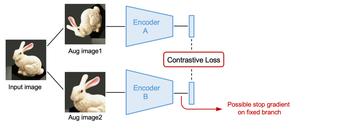
(a) General pipeline for contrastive learning from augmented data.

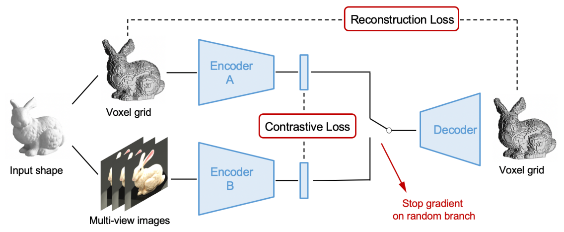
(b) Pipeline for the proposed generative-contrastive learning from multi-modal input.

Figure 1: An illustration of (a) a general pipeline of contrastive learning methods and (b) our proposed generative contrastive learning pipeline for 3D shapes.

When multi-modal input data is available, the question arises how to use them jointly. For 3D learning tasks, take 3D Euclidean data as an example, most state-of-the-art methods in computer vision that deal with both image and voxel grid input data either concatenate individual latent representations for supervised tasks [22], or use only one of them on the input and loss side separately [11, 40, 39, 45], or use them jointly but with pre-training and finetuning [15]. We are interested in seeking a better self-supervised way for learning better latent representations for 3D volumetric shapes, with the additional input from other modalities.

Apart from pretext tasks-based methods[14, 17], the other two main self-supervised learning ways are generative-based methods [1, 11] and contrastive-based methods [5, 18]. For 3D volumetric shapes, it is easy to implement a generative model. But it is still an open question that how to do it in a contrastive way, let alone the combination of these two. In a recent review paper of self-supervised learning [28], the authors argue that the only way of doing generative-contrastive learning is to train an encoder-decoder to generate synthetic samples and a discriminator to distinguish them from real samples. We disagree with this argument. In their definition, the discriminator is the contrastive part thus the model only focuses on negative pairs. We think it is also possible to use or only use positive pairs, e.g. in our case, using multi-modalities from the same input shape for two branches.

Figure 1 shows the main idea of our proposed generative-contrastive learning pipeline. Compared to the existing contrastive learning methods, our method shares some similarities with them while some significant differences also exist. Similarities are: (i) we both use a two-branches scheme to encode two inputs that origin from the same "raw data"; (ii) after getting encoded latent representations, we both compute a contrastive loss in the latent space; (iii) they use positive pairs for training (optionally with additional negative pairs), we also use positive pairs. Differences are: (i) they use different augmented data from the "raw data", while we use different modalities from the "raw data"; (ii) thus our network architectures of encoder A and B are not identical, while theirs are identical mostly; (iii) we add a decoder part and a reconstruction loss; (iv) they possibly have stop gradient on one fixed branch, while we do stop gradient on random branch with a switching scheme.

The main contributions of this paper are as follows:

• We propose a novel generative-contrastive learning pipeline for 3D volumetric shapes, which makes the joint training of encoders for multi-modal input data possible.

• With the switching scheme does the work of stopping gradient on random branch, model collapse is avoided. End-to-end training is also possible without the requirements of special pre-training.

• Better experimental results are achieved on both 3D shape reconstruction and classification tasks with our proposed model, compared to the results from the models which learn only on single-modal data.

• Using the voxel encoder as a self-supervised pre-trained feature extractor, we outperform 3D-GAN on the ModelNet40 classification task with a much shorter latent vector representations (128, compared to ca. 2.5 million dimensions in 3D-GAN).

• The voxel encoder pre-trained on one single category still performs surprisingly well as a feature extractor on the full dataset with other categories during the testing.

2 Related Work

Contrastive learning: The work of contrastive learning was pioneered by Yann LeCun’s group for face verification [10]. This topic is getting more and more popular recently since people find self-supervised learning are important for feature extraction and we now have really mature deep learning techniques. SimCLR [5] proposes to use two identical encoders for two branches, both positive pairs and negative pairs are used. MoCo [7] stops the gradient for the second branch, while using a momentum-based method to update the parameters of its encoder. SwAV [2] proposes to use a memory bank to get negative pairs out of the batch, the contrastive loss in their case is computed after clustering. For methods only use positive samples, BYOL [18] keeps the idea of momentum updating from MoCo, but adds an additional block in the first branch and only uses positive pairs. SimSiam [8] reports an observation of competitive results may still be achieved when modifying BYOL by making two encoders identical. A review of most relevant methods and their comparisons are given in [12].

Learning on 3D shapes with Euclidean data: For supervised tasks, VoxNet[30] is the pioneer to use 3D convolutional network to learn features from volumetric data for recognition. Its subsequent work of multi-level 3D CNN [13] learns multi-scale spatial features by considering multiple resolutions of the voxel input. Qi et al. [32] propose to use multi-resolution filtering in 3D for multi-view CNNs, as well as using subvolume supervision for auxiliary training. FusionNet [22] fuses three networks together: two VoxNets[30] and one MVCNN[37]. The three networks fuse at the score layers where a linear combination of scores is taken before the classification prediction.

For self-supervised tasks, ShapeNet [41] uses a reverse VoxNet to reconstruct 3D volumetric shapes from latent representations which are learned from depth maps. The T-L network [15] combines a 3D autoencoder with an image regressor to encode a unified vector representation given a 2D image. Autoencoders have also been widely use for 3D shape retrieval in other papers [44, 46]. Its variant, VAE, has been used in a similar way for 3D shape learning [1]. View information from images has also been widely investigated for 3D shape reconstruction. Choy et al. [11] proposed a framework named 3D-R2N2 to reconstruct 3D shapes from multi-view images by leveraging the power of recurrent neural networks [24]. [33] also uses a recurrent-based approach, but taking depth images as input. Some other methods use view information as auxiliary constraints [39, 45, 19]. Method uses GAN for 3D volumetric shape generation has been proposed in [40]. Some other latest works [31, 27] have also used multi-modal input data for joint end-to-end training, but they did not use a switching scheme.

We are aware that there are lots of other works applying deep learning-based methods on other 3D Non-Euclidean data formats, e.g. point clouds and meshes. But they are out of the scope of this work and we would like to leave them for future work.

3 Methodology

3.1 Generative-Contrastive Learning

Figure 1(b) shows the main idea of our proposed generative-contrastive learning pipeline. Similar to most existing contrastive learning methods, we use an architecture with two encoder branches to compute a contrastive loss between the latent representations from each branch. The inputs to two branches are the voxel grid and the multi-view images of an identical 3D shape. A generative decoder part is added to compute the reconstruction loss. The decoder is shared by two encoders and the two encoder branches are co-trained with the help of a switching scheme.

For contrastive learning methods, mode collapse is a big issue. Possible ways of dealing with it are adding additional blocks for encoder A, or stop gradient for encoder B and update its parameters in a momentum way slowly along with the updated parameters in encoder A. In our case, encoder A and B are already different network architectures thus the momentum method can not be applied, but we still managed to avoid model collapse successfully during the experiments. We attribute this success to two things: the reconstruction loss, and the switching scheme. The reconstruction loss has a strong supervision over the representational capacity of latent representations, while the switching scheme does the work of stopping gradient on random branch.

To further improve the latent representations, Variational Autoencoders (VAE) [26] are used instead of vanilla autoencoders. In a VAE, each input is mapped to a multivariate normal distribution around a point in the latent space, which makes a continuous latent space. A continuous latent space makes the smooth transition of 3D shapes possible with latent representations. The learned features are usually more smooth and meaningful.

3.2 Switch Encoding

When dealing with multi-modal inputs, most state-of-the-art methods just encode them separately into latent representations and then perform concatenation. Unlike them, we propose to use a switching scheme in the latent space to jointly train both encoders with a shared decoder. During the training, the switch is actuated for every training epoch with a preset probability to randomly select the encoded output from one encoder as the latent representation. This operation of switching between encoders continues during the whole end-to-end training.

The decoder is tasked to reconstruct the voxel representation of the 3D shape. Since the switched encoders are trained concurrently for the same decoder, they are forced to produce “mutually compatible” latent representations. The different input modalities result in different features that naturally emerge for the respective latent representation. For example, a voxel-based encoder is much more likely to generate an “overall volume” feature (simply the number of filled voxels) compared to a multi-view image encoder. By the cross-training with switched encoding, useful features for the latent representation can translate from one encoder to the other via the shared decoder. This results in improved latent representations also for the individual encoder when just one input modality is used after the training.

3.3 Loss Functions

The SwitchVAE loss functions consists of three parts: a reconstruction loss $L_{\mathrm{recon}}$, a KL divergence $L_{\mathrm{KL}}$ between latent representations and the normal prior distribution, and a contrastive loss $L_{\mathrm{contras}}$ between the latent representations from the different input formats. The overall network is parameterized by $\boldsymbol{\theta}=(\boldsymbol{\theta}_{\mathrm{vox}},\boldsymbol{\theta}_{\mathrm{img}},\boldsymbol{\theta}_{d})^{\top}$ for the voxel and image encoder and the voxel decoder respectively. The training samples are denoted $\boldsymbol{x}^{\alpha}$ for the input $\alpha\in\{\mathrm{img},\mathrm{vox}\}$. The switch value for $\alpha$ is randomly selected prior to every training epoch. The latent representations resulting from the VAE encoders are $(\boldsymbol{\mu}^{\alpha},\boldsymbol{\sigma}^{\alpha})=e^{\alpha}(\boldsymbol{x}^{\alpha})$. The latent representation is sampled for the current training epoch as $\boldsymbol{z}^{\alpha}\sim\mathcal{N}(\boldsymbol{\mu}^{\alpha},\boldsymbol{\sigma}^{\alpha})$. The decoder part is shared by both input modalities to reconstruct the voxel representation $\hat{\boldsymbol{x}}^{\alpha}=d(\boldsymbol{z}^{\alpha})$. Formally, the overall loss function decomposes into three terms

$$L_{\boldsymbol{\theta}}(\alpha,\boldsymbol{x}^{\mathrm{img}},\boldsymbol{x}^{\mathrm{vox}})={}$$ (1)

$$\qquad L_{\mathrm{recon}}(\boldsymbol{x}^{\mathrm{vox}},\hat{\boldsymbol{x}}^{\alpha})+\lambda_{\mathrm{KL}}L_{\mathrm{KL}}(\boldsymbol{\mu}^{\alpha},\boldsymbol{\sigma}^{\alpha})+{}$$

$$\qquad\lambda_{\mathrm{contras}}L_{\mathrm{contras}}(\boldsymbol{z}^{\mathrm{img}},\boldsymbol{z}^{\mathrm{vox}})$$

with weights $\lambda_{\mathrm{KL}}$ and $\lambda_{\mathrm{contras}}$.

A modified Binary Cross Entropy (BCE) against the voxel ground truth is used for the reconstruction loss. To improve the training, modification has been made by the introduction of a hyper-parameter $\gamma$ that weights the relative importance of false positives against false negatives. The reconstructed voxels are indexed by $k$ with value $\hat{x}^{\alpha}_{k}\in[0,1]$.

$$L_{\mathrm{recon}}(\boldsymbol{x}^{\mathrm{vox}},\hat{\boldsymbol{x}}^{\alpha}) {}=\sum_{k}\Big{[}-\gamma\cdot x^{\mathrm{vox}}_{k}\cdot\log(\hat{x}^{\alpha}_{k})-{}$$ (2)

$$(1-\gamma)(1-x^{\mathrm{vox}}_{k})\log(1-\hat{x}^{\alpha}_{k})\Big{]}$$

We set the hyperparameter $\gamma=0.8$ during training for all of the experiments conducted in Section 4.

In the training of VAE, the Kullback-Leibler (KL) divergence is used between the actual distribution of latent vectors and the $\mathcal{N}(\boldsymbol{0},I)$ Gaussian distribution. Note that the latent representation has $n$ dimensions.

$$L_{\mathrm{KL}}(\boldsymbol{\mu},\boldsymbol{\sigma})=-\frac{1}{2}\sum_{i=1}^{n}(1+\log(\sigma_{i}^{2})-\mu_{i}^{2}-\sigma_{i}^{2})$$ (3)

In order to further force a close distance between the latent representations learned from image and volumetric data with the SwitchVAE model, a contrastive loss between the encoders is proposed and used in the latent space during the training phase. The contrastive loss is defined as the Euclidean distance between the latent vectors from images and volumetric data.

$$L_{\mathrm{contras}}(\boldsymbol{z}^{\mathrm{img}},\boldsymbol{z}^{\mathrm{vox}})=\|\boldsymbol{z}^{\mathrm{img}}-\boldsymbol{z}^{\mathrm{vox}}\|_{2}^{2}$$ (4)

Although in most other contrastive learning methods some different contrastive losses has been used, e.g. InfoNCE loss in SimCLR [5], we find that with latent representations normalized, our method can already yield satisfying results with a simple $L_{2}$ Norm loss as the contrastive loss.

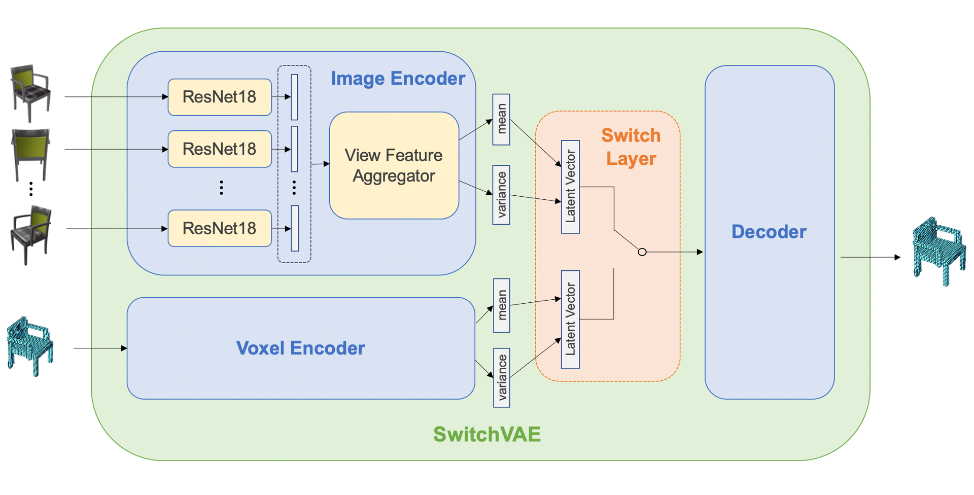
Figure 2: The SwitchVAE architecture based on our proposed generative-contrastive learning pipeline, with more detail blocks illustrated.

Input/GT

Voxel VAE

SwitchVAE

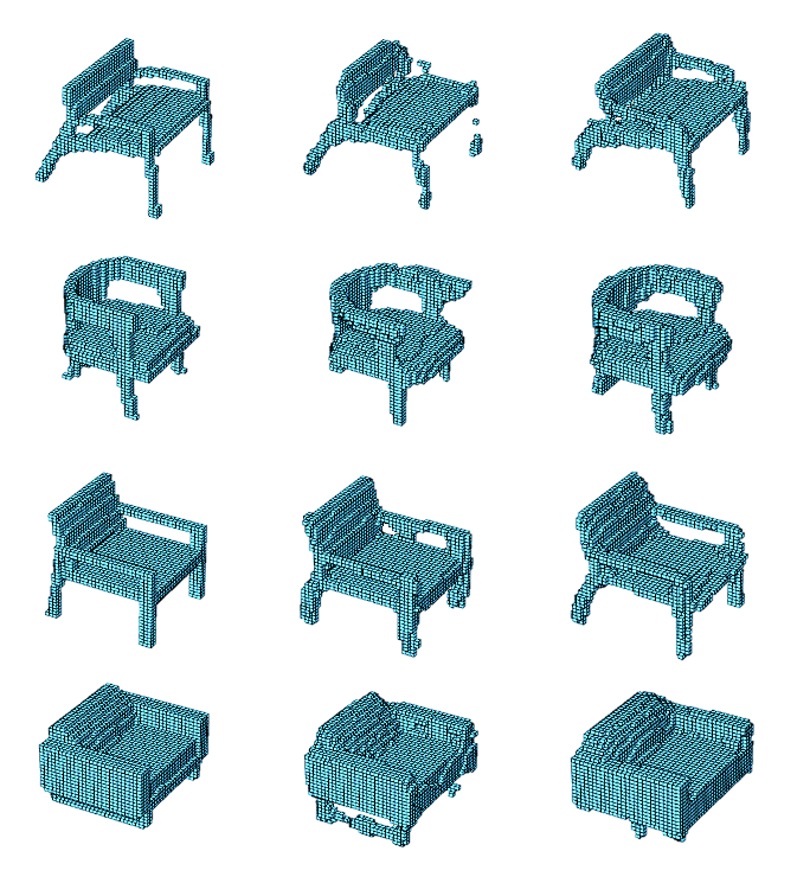
(a) Reconstruction tests with voxel input.

Input (2/8 views)

GT

Image VAE

SwitchVAE

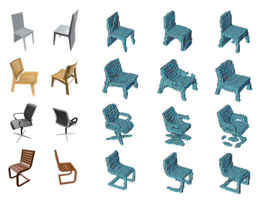
(b) Reconstruction tests with image input.

Figure 3: Some reconstruction results from different models with only voxel or multi-view images as the test input.

Test Input	Training Model	Reconstruction Metrics
		IoU	Precision	Accuracy
Image	Image VAE	58.52%	68.21%	93.21%
	SwitchVAE ($\lambda_{\mathrm{contras}}=0$)	56.82%	67.72%	93.00%
	SwitchVAE ($\lambda_{\mathrm{contras}}=1$)	58.75%	68.50%	93.32%
Voxel	Voxel VAE	78.86%	82.80%	97.01%
	SwitchVAE ($\lambda_{\mathrm{contras}}=0$)	77.27%	80.04%	96.67%
	SwitchVAE ($\lambda_{\mathrm{contras}}=1$)	79.93%	84.68%	97.22%

Table 1: Reconstruction performance on the test set. Training and testing with the chair category from 3D-R2N2 dataset.

4 Experiments

We use the 3D-R2N2 and ModelNet 10/40 datasets for our experiments. The 3D-R2N2 dataset [11] is a subset with 13 categories from the ShapeNet dataset [3]. It provides good quality rendered multi-view images alongside a class label and $32\times 32\times 32$ voxel representations. We divide the 3D-R2N2 dataset into a training set of 29,599 samples and a test set of 7406 samples. The ModelNet dataset [41] comes in two variations with either 10 or 40 classes of shapes. The ModelNet10 dataset contains 3991/908 training/test samples. ModelNet40 contains 9843/2468 training/test samples.

For the SwitchVAE models, we use both a voxel and a multi-view image encoder. The decoder always reconstructs the voxel representation. During training for voxel test input, the switch layer randomly selects either the voxel encoder with a probability of 80%, or the multi-view image encoder with a probability of 20%.

Concerning the other training parameters, we use a latent dimension of 128 for all experiments. The network parameters are trained by minimizing the loss function from Equation 1 using the SGD optimizer with a momentum of 0.9 and Nesterov accelerated gradients [34]. The learning rate is $2\times 10^{-4}$ with a decay of 0.96 per 10 epochs after the first 50 epochs. The batch size is 32 for all experiments. Training with multi-view image input uses 8 views for every sample as it has been reported in [11] and its subsequent works [42, 43] that the improvement from additional views is negligible after the first 6-10 views.

4.1 Detailed Network Configuration

Figure 2 shows based on our proposed generative-contrastive learning pipeline, how switched encoding is implemented for a VAE with multi-view images and voxel grids input. The encoder blocks of our SwitchVAE build on the idea of volumetric convolutional networks [41] for the voxel input, and 3D recurrent reconstruction neural networks [11] for the multi-view images input. More detailed network configurations are given as follows.

The image encoder of SwitchVAE learns the latent vector from multi-view images, and it is composed of a view feature embedding module and a view feature aggregator module. The view feature embedding module is a ResNet18 [21] whose weights are shared across all the views. The part with pre-trained weights map a single view $137\times 137\times 3$ RGB image into $5\times 5\times 512$ feature maps. We then flatten these feature maps and add a fully connected layer, which outputs a 1024 dimensional feature for a single view image. For a 3D shape, 8 views of images are fed into the shared weights view feature embedding module while training, which outputs a $8\times 1024$ view features.

For the view feature aggregator module, we firstly tried a max pooling as MVCNN [37], but it did not yield satisfying results. Same for average pooling. To better aggregate the multi-view image features, we finally use the Gated Recurrent Unit (GRU) [9]. The view feature aggregator outputs a 1024 dimensional feature after aggregating features from all views. Then it is further fed into last fully connected layers to generate the mean and the variance of the latent vector. By using the reparametrization trick introduced in [25], the image encoder finally outputs a 128 dimensional sampled latent vector.

The voxel encoder is a 3D volumetric convolutional neural network. The encoder has 4 convolutional layer and two fully connected layers. All convolutional layers use kernels of size $3\times 3\times 3$, their strides are $\{1,2,1,2\}$ and channel numbers are $\{8,16,32,64\}$ respectively. All layers use the exponential linear unit (eLu) as the activation function except for the last fully connected layer. This layer maps an shape of $32\times 32\times 32$ voxels to a 343 dimensional feature. The 343 dimensional feature is further fed into the last fully connected layers to generate the mean and the variance of the latent vector to finally produce a 128 dimensional sampled latent vector.

The decoder of SwitchVAE mirrors the voxel encoder, except that the last layer uses a sigmoid activation function. The decoder maps a 128 dimensional latent vector, which was randomly sampled in encoder, to a $32\times 32\times 32$ volumetric reconstruction. It represents the predicted voxel occupancy possibility of each voxel in the cube.

4.2 3D Shape Reconstruction

We use Intersection-of-Union (IoU), precision, recall, and accuracy (referred as average precision in [15]) as the quantitative metrics for the reconstruction of 3D shapes. The threshold at which a voxel is considered as filled is at 50%. Similar to the last part, we show the results from only voxel input training, only image input training, and both input training with our SwitchVAE.

Table 1 shows that the reconstruction performance of SwitchVAE is similar or slightly better to that of image/voxel VAEs, and it focuses more on making every predicted occupied voxel correct (higher precision score). This characteristic may be more clearly observed in some reconstruction results. Table 1 also shows that the contrastive loss term is the key in our method. Figure 3 shows some qualitative reconstruction results from our SwitchVAE model that trained on the chair category. Comparisons with the results from the networks that only use one input format for training are also presented. From the figure we can observe that SwitchVAE takes more attention on not occupying original negative voxels. This is quite obvious from the third row of Figure 3(b). Both Image VAE and SwitchVAE are not certain about the leg number of the office chair is 4 or 5. The Image VAE decides to merge them all together, while SwitchVAE decides to only guess and occupy some voxels with small sub-clusters in that area.

Training Dataset	Test Input	Training Model	Classification Accuracy
			ModelNet40	ModelNet10
Chair Category	Multi-view images	Image VAE	75.28%	81.36%
		SwitchVAE	77.07%	84.26%
	Voxel data	Voxel VAE	80.19%	86.38%
		SwitchVAE	80.60%	87.05%
ModelNet40	Multi-view images	Image VAE	85.06%	88.62%
		SwitchVAE	83.87%	89.96%
	Voxel data	Voxel VAE	83.12%	87.95%
		SwitchVAE	84.01%	90.07%

Table 2: Classification accuracy on the ModelNet40/ModelNet10 classification tasks with models trained with Image VAE, Voxel VAE, and SwitchVAE on the chair category or on the full ModelNet40 dataset.

Supervision	Method	Data Modality	Classification Accuracy
			ModelNet40	ModelNet10
Supervised	3D ShapNets [41]	Voxels	77.30%	85.30%
	VoxNet [30]	Voxels	83.00%	92.00%
	MVCNN [37]	Images	90.10%	-
	FusionNets [22]	Images, Voxels	90.80%	93.11%
	3D2SeqViews [20]	Images	93.40%	94.71%
	VRN Ensemble [1]	Voxels	95.54%	97.14%
Self-supervised	LFD [4]	Images	75.50%	79.90%
	T-L Network [15]	Images, Voxels	74.40%	-
	VConv-DAE [35]	Voxels	75.50%	80.50%
	3D GAN [40]	Voxels	83.30%	91.00%
	SwitchVAE (trained on only chair category)	Images, Voxels	80.60%	87.05%
	SwitchVAE (trained on ModelNet40 dataset)	Images, Voxels	84.01%	90.07%

Table 3: Classification accuracy on the ModelNet40/ModelNet10 dataset with different methods. Results from methods that only used images and/or voxels are listed. Note that our latent representations are only of 128 dimensions.

4.3 3D Shape Classification

For the classification task, the networks are first trained to perform reconstruction of the ground-truth voxel representations. Then the encoder part of a trained network is used to produce latent representations of 128 dimensions as input for classification. An SVM with RBF kernel and hyper-parameter $\gamma=1/128$ is trained on the latent representations to perform classification. Same samples were used to train the networks for latent representations and the SVM. The evaluation of the SVM is performed with samples that were neither used to train the networks nor the SVM.

Table 2 shows the impact of switched training on the ModelNet 10/40 classification tasks. To make it more clear, let’s take the voxel data testings as an example. During the training phase, a voxel VAE only trains on the voxel train set data, while a SwitchVAE trains on both the voxel train set data and the correspondent multi-view images train set data. During the testing phase, only the identical voxel test set data is given to the trained voxel VAE model and the trained SwitchVAE model. Latent representations of those 3D shapes (from voxel test set) obtained from the SwitchVAE model always outperform that from the vanilla voxel VAE in the ModelNet classification tasks. Note that no multi-view images data of the test set is needed for SwitchVAE during the testings. From Table 2, we can clearly observe that under the condition of same training dataset and test input, the results from SwitchVAE are better than the results from the image VAE or the voxel VAE in most cases. Note that they are even trained with a same number of epochs. This means by using the data of other format in the training phase, during the testing phase, the classification performance has been improved compared to the models that only use single format for the training. In conclusion, better latent representations have been learned for 3D shapes by using “data you don’t have” (i.e. data input formats that are not used for the evaluation once the network is trained).

Table 3 lists the classification result in comparison to other network architectures. Compared to most other unsupervised learning method, we achieve better classification performance. Comparing to 3D-GAN, we outperform it on the ModelNet40 classification task and achieve competitive performance on the ModelNet10 classification task. However, our method uses a much smaller latent vector of only 128 dimensions. 3D-GANs use all features maps in the last three convolution layers, which makes the presentation for each 3D shape a 2.5 million dimensional vector as input for the classification.

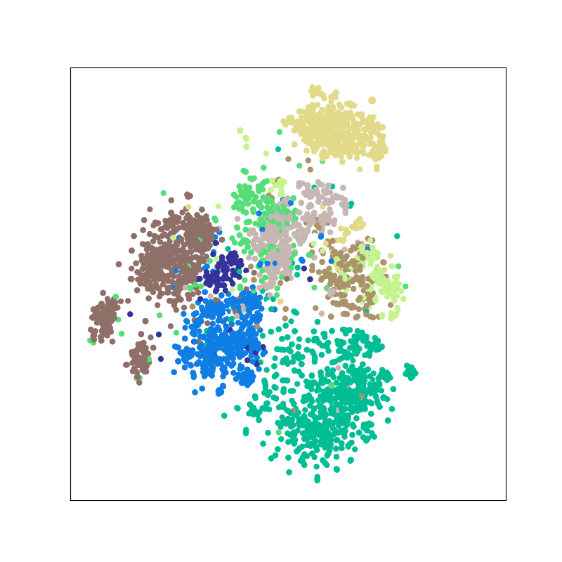
(a)   Voxel VAE,
trained on ModelNet10

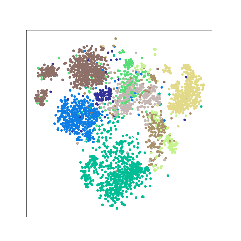
(b) SwitchVAE ($\lambda_{\mathrm{contras}}=0$),
trained on ModelNet10

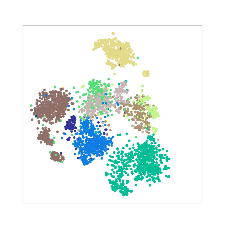
(c) SwitchVAE ($\lambda_{\mathrm{contras}}=1$),
trained on ModelNet10

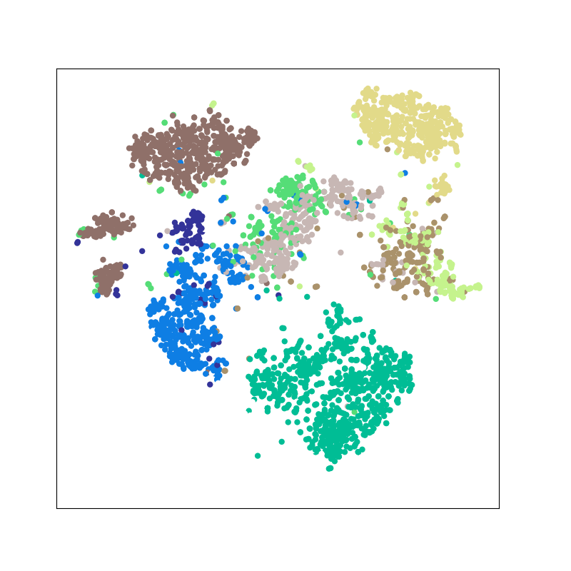
(d) SwitchVAE ($\lambda_{\mathrm{contras}}=1$),
trained on 3D-R2N2 dataset

Figure 4: t-SNE plots of the latent representations for ModelNet10 shapes (10 categories) with (a) a vanilla voxel VAE model trained on ModelNet10 dataset. (b) a SwitchVAE model without contrastive loss trained on ModelNet10 dataset. (c) a SwitchVAE model with contrastive loss trained on ModelNet10 dataset. (d) a SwitchVAE model with contrastive loss trained on the full 3D-R2N2 dataset. Each color represents one category. All latent representations used for the plots use voxel data from the testing set as test input.

t-SNE Visualization: In order to visualize the learned latent representations, we use t-SNE [29] to map the latent representations to a 2D plane. Figure 4 gives the visualization results. we use ModelNet10 for most t-SNE visualization experiments. Comparing Figure 4(a) and Figure 4(b), we can observe that the switching scheme contributes to the inter-category classification while makes the intra-category clustering a bit fuzzy (all categories are a bit far from each other, while each category itself is a bit less clustered). Comparing Figure 4(b) and Figure 4(c), we can observe that adding the contrastive loss term to SwitchVAE helps to the intra-category clustering, making the performance of the whole classification task mush better. Comparing Figure 4(c) and Figure 4(d), we can observe that with a larger training dataset, even better feature clustering results may be achieved. The increased gaps between different categories can be clearly observed.

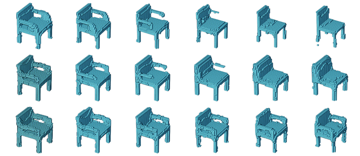
(a) Top Row: Trained on SwitchVAE, the "chair arm" feature and the “size” feature are entangled. Middle and Bottom Row: Trained on Switch-BetaTCVAE with $\beta=5$, the “chair arm” feature and the “size” feature are more disentangled, changing one feature does not impact the other one too much.

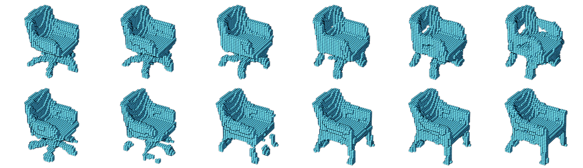
(b) Top Row: Trained on SwitchVAE, changing the “chair leg type” feature also leads to the morphing of the top part. Bottom Row: Trained on Switch-BetaTCVAE with $\beta=5$, the top part stays more fixed while changing the “chair leg type” feature.

Figure 5: Disentangling latent features with Beta-TCVAE.

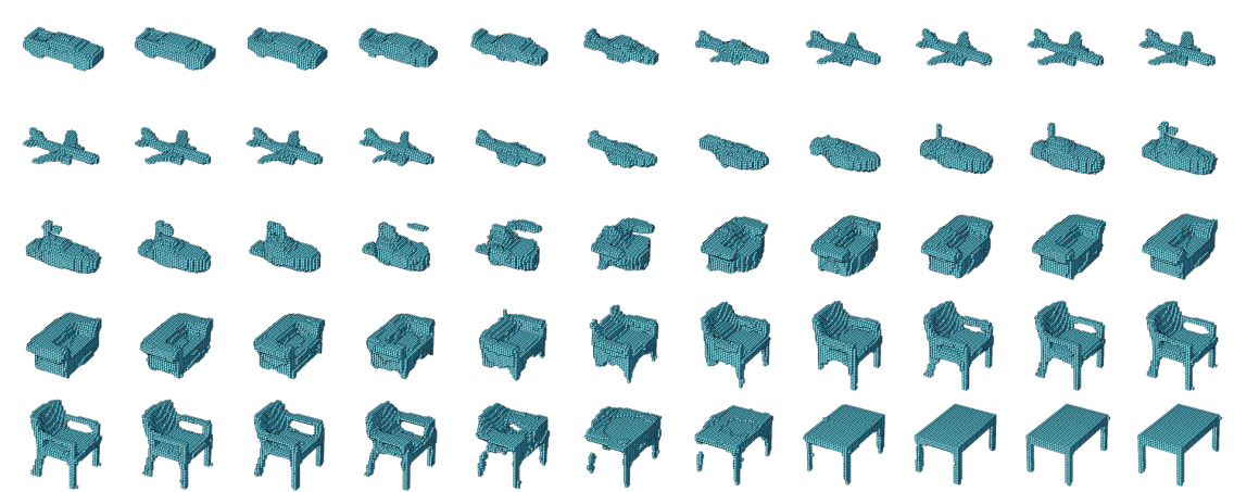
Figure 6: Shape interpolation between different categories.

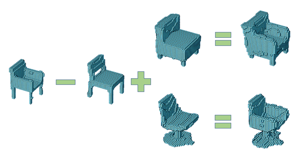
(a) Shape arithmetic example with chair objects.

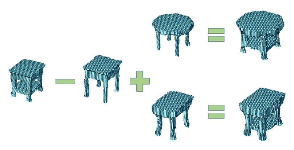
(b) Shape arithmetic example with table objects.

Figure 7: Shape arithmetic for chairs and tables. (a) Adding chair arms to chair objects in the latent space. (b) Adding a middle layer to table objects in the latent space.

4.4 Exploring Latent Representations

This subsection showcases some qualitative results to give indication that SwitchVAE training results in a superior latent representation that allows for better disentanglement between categories, as well as between the salient features of the 3D shapes in each category.

Latent space interpolation: Similar to as most 3D reconstruction papers, we also do the inter-class interpolation with our trained models as shown in Figure 6. It can be observed that our proposed method has the ability to do smooth transition between two shapes, even if they are from different categories.

Shape arithmetic: Another way to explore the learned latent representations is to perform arithmetic operations in the latent space whilst observing their effect on the reconstructed geometry. We show some shape arithmetic results in Figure 7 with a model trained on the full 3D-R2N2 dataset. The model seems to capture the underline information and is capable of generating meaningful combined shapes that do not occur as 3D shapes in the original dataset.

Feature disentanglement with VAE variations: One good thing with VAE models is that the latent space learned from it is more "meaningful" comparing to that from GAN models. By tuning the value in one specific latent dimension, one can observe certain features on the output side changing smoothly. However, for most features, they get entangled in multiple latent dimensions with the vanilla VAE. It has been reported that $\beta$-VAE [23] and $\beta$-TCVAE [6] can producing better disentangled features in the latent space. We merge it with our proposed method into SwitchBTCVAE. We train our model with $\beta=5$ on the chair category with a same number of epochs as the other experiments shown in this section. Although a small decrease on the reconstruction performance metrics is observed, by investigating the learned latent representations, we find that some features have been better disentangled as shown in Figure 5.

5 Conclusion and Outlook

In this paper, we propose a generative-contrastive learning pipeline for learning better latent representations for 3D volumetric shapes, with the help of additional modality input. The switching scheme makes the joint training for both encoders possible with competitive reconstruction results. Classification experiments on ModelNet have also been carried out to validate the effectiveness of the proposed method. Improved classification results indicate that better latent representations have been learned with our proposed SwitchVAE architecture.

For future directions, other 3D data modalities, e.g., point clouds and meshes may also be used. A new contrastive loss may be designed and an optimal switching policy may be studied. More researches may be conducted to make the latent presentations more feature disentangled or more interpretable. In our experiments, although an additional contrastive loss has been applied, we still observe large distances between latent representations generated from the different input formats. An understanding how to force a close distance between representations without leading to a collapse from an increased contrastive loss would lead to more insight into contrastive learning itself.

References

- [1] A. Brock, T. Lim, J. M. Ritchie, and N. Weston. Generative and discriminative voxel modeling with convolutional neural networks. NeurIPS, 2016.
- [2] M. Caron, I. Misra, J. Mairal, P. Goyal, P. Bojanowski, and A. Joulin. Unsupervised learning of visual features by contrasting cluster assignments. NeurIPS, 2020.
- [3] A. X. Chang, T. Funkhouser, L. Guibas, P. Hanrahan, Q. Huang, Z. Li, S. Savarese, M. Savva, S. Song, H. Su, J. Xiao, L. Yi, and F. Yu. Shapenet: An information-rich 3d model repository. ArXiv, abs/1512.03012, 2015.
- [4] D. Chen, X. Tian, E. Shen, and M. Ouhyoung. On visual similarity based 3d model retrieval. Computer Graphics Forum, 22, 2003.
- [5] T. Chen, S. Kornblith, M. Norouzi, and G. E. Hinton. A simple framework for contrastive learning of visual representations. ICML, 2020.
- [6] T. Q. Chen, X. Li, R. B. Grosse, and D. Duvenaud. Isolating sources of disentanglement in variational autoencoders. 2018.
- [7] X. Chen, H. Fan, R. B. Girshick, and K. He. Improved baselines with momentum contrastive learning. CVPR, 2020.
- [8] X. Chen and K. He. Exploring simple siamese representation learning. CVPR, 2021.
- [9] K. Cho, B. V. Merrienboer, C. Gülçehre, D. Bahdanau, F. Bougares, H. Schwenk, and Y. Bengio. Learning phrase representations using rnn encoder-decoder for statistical machine translation. ArXiv, abs/1406.1078, 2014.
- [10] S. Chopra, R. Hadsell, and Y. LeCun. Learning a similarity metric discriminatively, with application to face verification. CVPR, pages 539--546, 2005.
- [11] C. Choy, D. Xu, J. Gwak, K. Chen, and S. Savarese. 3d-r2n2: A unified approach for single and multi-view 3d object reconstruction. ECCV, 2016.
- [12] L. Ericsson, H. Gouk, and T. M. Hospedales. How well do self-supervised models transfer? CVPR, 2021.
- [13] S. Ghadai, X. Lee, A. Balu, S. Sarkar, and A. Krishnamurthy. Multi-level 3d cnn for learning multi-scale spatial features. IEEE/CVF Conference on Computer Vision and Pattern Recognition Workshops (CVPRW), pages 1152--1156, 2019.
- [14] S. Gidaris, P. Singh, and N. Komodakis. Unsupervised representation learning by predicting image rotations. ICLR, 2018.
- [15] R. Girdhar, D. F. Fouhey, M. Rodriguez, and A. Gupta. Learning a predictable and generative vector representation for objects. ECCV, 2016.
- [16] I. J. Goodfellow, Y. Bengio, and A. C. Courville. Deep learning. Nature, 521:436--444, 2015.
- [17] P. Goyal, D. Mahajan, A. Gupta, and I. Misra. Scaling and benchmarking self-supervised visual representation learning. ICCV, 2019.
- [18] J. Grill, F. Strub, F. Altch’e, C. Tallec, P. H. Richemond, E. Buchatskaya, C. Doersch, B. A. Pires, Z. Guo, M. G. Azar, B. Piot, K. Kavukcuoglu, R. Munos, and M. Valko. Bootstrap your own latent: A new approach to self-supervised learning. NeurIPS, 2020.
- [19] J. Gwak, C. B. Choy, M. Chandraker, A. Garg, and S. Savarese. Weakly supervised 3d reconstruction with adversarial constraint. 2017 International Conference on 3D Vision (3DV), pages 263--272, 2017.
- [20] Z. Han, H. Lu, Z. Liu, C. Vong, Y. Liu, M. Zwicker, J. Han, and C. Chen. 3d2seqviews: Aggregating sequential views for 3d global feature learning by cnn with hierarchical attention aggregation. IEEE Transactions on Image Processing, 28:3986--3999, 2019.
- [21] K. He, X. Zhang, S. Ren, and J. Sun. Deep residual learning for image recognition. CVPR, pages 770--778, 2016.
- [22] V. Hegde and R. Zadeh. Fusionnet: 3d object classification using multiple data representations. ArXiv, abs/1607.05695, 2016.
- [23] I. Higgins, L. Matthey, A. Pal, C. Burgess, X. Glorot, M. Botvinick, S. Mohamed, and A. Lerchner. beta-vae: Learning basic visual concepts with a constrained variational framework. In ICLR, 2017.
- [24] S. Hochreiter and J. Schmidhuber. Long short-term memory. Neural Computation, 9:1735--1780, 1997.
- [25] D. P. Kingma and M. Welling. Auto-encoding variational bayes. CoRR, abs/1312.6114, 2014.
- [26] D. P. Kingma and M. Welling. An introduction to variational autoencoders. Foundations and Trends in Machine Learning, 12:307--392, 2019.
- [27] R. Klokov, J. Verbeek, and E. Boyer. Probabilistic reconstruction networks for 3d shape inference from a single image. 2019.
- [28] X. Liu, F. Zhang, Z. Hou, Z. Wang, L. Mian, J. Zhang, and J. Tang. Self-supervised learning: Generative or contrastive. IEEE Transactions on Knowledge and Data Engineering, 2020.
- [29] L. V. D. Maaten and G. E. Hinton. Visualizing data using t-sne. Journal of Machine Learning Research, 9:2579--2605, 2008.
- [30] D. Maturana and S. Scherer. Voxnet: A 3d convolutional neural network for real-time object recognition. IEEE/RSJ International Conference on Intelligent Robots and Systems (IROS), pages 922--928, 2015.
- [31] S. Muralikrishnan, V. G. Kim, M. Fisher, and S. Chaudhuri. Shape unicode: A unified shape representation. CVPR, pages 3785--3794, 2019.
- [32] C. R. Qi, H. Su, M. Nießner, A. Dai, M. Yan, and L. Guibas. Volumetric and multi-view cnns for object classification on 3d data. CVPR, pages 5648--5656, 2016.
- [33] D. J. Rezende, S. Eslami, S. Mohamed, P. Battaglia, M. Jaderberg, and N. Heess. Unsupervised learning of 3d structure from images. 2016.
- [34] S. Ruder. An overview of gradient descent optimization algorithms. ArXiv, abs/1609.04747, 2016.
- [35] A. Sharma, O. Grau, and M. Fritz. Vconv-dae: Deep volumetric shape learning without object labels. ArXiv, abs/1604.03755, 2016.
- [36] O. Sorkine-Hornung. Laplacian mesh processing. Eurographics, 2005.
- [37] H. Su, S. Maji, E. Kalogerakis, and E. Learned-Miller. Multi-view convolutional neural networks for 3d shape recognition. ICCV, pages 945--953, 2015.
- [38] J. Sun, M. Ovsjanikov, and L. Guibas. A concise and provably informative multi‐scale signature based on heat diffusion. Computer Graphics Forum, 28, 2009.
- [39] S. Tulsiani, A. A. Efros, and J. Malik. Multi-view consistency as supervisory signal for learning shape and pose prediction. CVPR, pages 2897--2905, 2018.
- [40] J. Wu, C. Zhang, T. Xue, B. Freeman, and J. Tenenbaum. Learning a probabilistic latent space of object shapes via 3d generative-adversarial modeling. ArXiv, abs/1610.07584, 2016.
- [41] Z. Wu, S. Song, A. Khosla, F. Yu, L. Zhang, X. Tang, and J. Xiao. 3d shapenets: A deep representation for volumetric shapes. CVPR, pages 1912--1920, 2015.
- [42] H. Xie, H. Yao, X. Sun, S. Zhou, S. Zhang, and X. Tong. Pix2vox: Context-aware 3d reconstruction from single and multi-view images. ICCV, pages 2690--2698, 2019.
- [43] H. Xie, H. Yao, S. Zhang, S. Zhou, and W. Sun. Pix2vox++: Multi-scale context-aware 3d object reconstruction from single and multiple images. International Journal of Computer Vision, pages 1 -- 17, 2020.
- [44] J. Xie, Yi Fang, F. Zhu, and E. K. Wong. Deepshape: Deep learned shape descriptor for 3d shape matching and retrieval. CVPR, pages 1275--1283, 2015.
- [45] X. Yan, J. Yang, E. Yumer, Y. Guo, and H. Lee. Perspective transformer nets: Learning single-view 3d object reconstruction without 3d supervision. 2016.
- [46] Z. Zhu, X. Wang, S. Bai, C. Yao, and X. Bai. Deep learning representation using autoencoder for 3d shape retrieval. IEEE International Conference on Security, Pattern Analysis, and Cybernetics (SPAC), pages 279--284, 2014.