Federated Learning under Heterogeneous and Correlated Client Availability

Abstract

The enormous amount of data produced by mobile and IoT devices has motivated the development of federated learning (FL), a framework allowing such devices (or clients) to collaboratively train machine learning models without sharing their local data. FL algorithms (like FedAvg) iteratively aggregate model updates computed by clients on their own datasets. Clients may exhibit different levels of participation, often correlated over time and with other clients. This paper presents the first convergence analysis for a FedAvg-like FL algorithm under heterogeneous and correlated client availability. Our analysis highlights how correlation adversely affects the algorithm’s convergence rate and how the aggregation strategy can alleviate this effect at the cost of steering training toward a biased model. Guided by the theoretical analysis, we propose CA-Fed, a new FL algorithm that tries to balance the conflicting goals of maximizing convergence speed and minimizing model bias. To this purpose, CA-Fed dynamically adapts the weight given to each client and may ignore clients with low availability and large correlation. Our experimental results show that CA-Fed achieves higher time-average accuracy and a lower standard deviation than state-of-the-art AdaFed and F3AST, both on synthetic and real datasets.

I Introduction

The enormous amount of data generated by mobile and IoT devices motivated the emergence of distributed machine learning training paradigms [1, 2]. Federated Learning (FL) [3, 4, 5, 6] is an emerging framework where geographically distributed devices (or clients) participate in the training of a shared Machine Learning (ML) model without sharing their local data. FL was proposed to reduce the overall cost of collecting a large amount of data as well as to protect potentially sensitive users’ private information. In the original Federated Averaging algorithm (FedAvg) [4], a central server selects a random subset of clients from the set of available clients and broadcasts them the shared model. The sampled clients perform a number of independent Stochastic Gradient Descent (SGD) steps over their local datasets and send their local model updates back to the server. Then, the server aggregates the received client updates to produce a new global model, and a new training round begins. At each iteration of FedAvg, the server typically samples randomly a few hundred devices to participate [7, 8].

In real-world scenarios, the availability/activity of clients is dictated by exogenous factors that are beyond the control of the orchestrating server and hard to predict. For instance, only smartphones that are idle, under charge, and connected to broadband networks are commonly allowed to participate in the training process [4, 9]. These eligibility requirements can make the availability of devices correlated over time and space [7, 10, 11, 12]. For example, temporal correlation may origin from a smartphone being under charge for a few consecutive hours and then ineligible for the rest of the day. Similarly, the activity of a sensor powered by renewable energy may depend on natural phenomena intrinsically correlated over time (e.g., solar light). Spatial correlation refers instead to correlation across different clients, which often emerges as consequence of users’ different geographical distribution. For instance, clients in the same time zone often exhibit similar availability patterns, e.g., due to time-of-day effects.

Temporal correlation in the data sampling procedure is known to negatively affect the performance of ML training even in the centralized setting [13, 14] and can potentially lead to catastrophic forgetting: the data used during the final training phases can have a disproportionate effect on the final model, “erasing” the memory of previously learned information [15, 16]. Catastrophic forgetting has also been observed in FL, where clients in the same geographical area have more similar local data distributions and clients’ participation follows a cyclic daily pattern (leading to spatial correlation) [7, 10, 11, 17]. Despite this evidence, a theoretical study of the convergence of FL algorithms under both temporally and spatially correlated client participation is still missing.

This paper provides the first convergence analysis of FedAvg [4] under heterogeneous and correlated client availability. We assume that clients’ temporal and spatial availability follows an arbitrary finite-state Markov chain: this assumption models a realistic scenario in which the activity of clients is correlated and, at the same time, still allows the analytical tractability of the system. Our theoretical analysis (i) quantifies the negative effect of correlation on the algorithm’s convergence rate through an additional term, which depends on the spectral properties of the Markov chain; (ii) points out a trade-off between two conflicting objectives: slow convergence to the optimal model, or fast convergence to a biased model, i.e., a model that minimizes an objective function different from the initial target. Guided by insights from the theoretical analysis, we propose CA-Fed, an algorithm which dynamically assigns weights to clients and achieves a good trade-off between maximizing convergence speed and minimizing model bias. Interestingly, CA-Fed can decide to ignore clients with low availability and high temporal correlation. Our experimental results demonstrate that excluding such clients is a simple, but effective approach to handle the heterogeneous and correlated client availability in FL. Indeed, while CA-Fed achieves a comparable maximum accuracy as the state-of-the-art methods F3AST [18] and AdaFed [19], its test accuracy exhibits higher time-average and smaller variability over time.

The remainder of this paper is organized as follows. Section II describes the problem of correlated client availability in FL and discusses the main related works. Section III provides a convergence analysis of FedAvg under heterogeneous and correlated client participation. CA-Fed, our correlation-aware FL algorithm, is presented in Section IV. We evaluate CA-Fed in Section V, comparing it with state-of-the-art methods on synthetic and real-world data. Section VII concludes the paper.

II Background and Related Works

We consider a finite set $\mathcal{K}$ of $N$ clients. Each client $k\in\mathcal{K}$ holds a local dataset $D_{k}$. Clients aim to jointly learn the parameters $\bm{w}\in W\subseteq\mathbb{R}^{d}$ of a global ML model (e.g., the weights of a neural network architecture). During training, the quality of the model with parameters $\bm{w}$ on a data sample $\xi\in D_{k}$ is measured by a loss function $f(\bm{w};\xi)$. The clients solve, under the orchestration of a central server, the following optimization problem:

$$\min_{\bm{w}\in W\subseteq\mathbb{R}^{d}}\left[F(\bm{w})\coloneqq\sum_{k\in\mathcal{K}}\alpha_{k}F_{k}(\bm{w})\right],$$ (1)

where $F_{k}(\bm{w})\coloneqq\frac{1}{|D_{k}|}\sum_{\xi\in D_{k}}f(\bm{w};\xi)$ is the average loss computed on client $k$’s local dataset, and $\bm{\alpha}=(\alpha_{k})_{k\in\mathcal{K}}$ are positive coefficients such that $\sum_{k}\alpha_{k}=1$. They represent the target importance assigned by the central server to each client $k$. Typically $(\alpha_{k})_{k\in\mathcal{K}}$ are set proportional to the clients’ dataset size $|D_{k}|$, such that the objective function $F$ in (1) coincides with the average loss computed on the union of the clients’ local datasets $D=\cup_{k\in\mathcal{K}}D_{k}$.

Under proper assumptions, precised in Section III, Problem (1) admits a unique solution. We use $\bm{w}^{*}$ (resp. $F^{*}$) to denote the minimizer (resp. the minimum value) of $F$. Moreover, for ${\color[rgb]{0,0,0}k{\in}\mathcal{K}}$, $F_{k}$ admits a unique minimizer on $W$. We use $\bm{w}_{k}^{*}$ (resp. $F_{k}^{*}$) to denote the minimizer (resp. the minimum value) of $F_{k}$.

Problem (1) is commonly solved through iterative algorithms [4, 8] requiring multiple communication rounds between the server and the clients. At round $t>0$, the server broadcasts the latest estimate of the global model $\bm{w}_{t,0}$ to the set of available clients ($A_{t}$). Client $k\in A_{t}$ updates the global model with its local data through $E\geq 1$ steps of local Stochastic Gradient Descent (SGD):

$$\textstyle\bm{w}_{t,j+1}^{k}=\bm{w}_{t,j}^{k}-\eta_{t}\nabla F_{k}(\bm{w}_{t,j}^{k},\mathcal{B}_{t,j}^{k})\quad j=0,\dots,E-1,$$ (2)

where $\eta_{t}>0$ is an appropriately chosen learning rate, referred to as local learning rate; $\mathcal{B}_{t,j}^{k}$ is a random batch sampled from client $k$’ local dataset at round $t$ and step $j$; $\nabla F_{k}(\cdot,\mathcal{B})\coloneqq\frac{1}{|\mathcal{B}|}\sum_{\xi\in\mathcal{B}}\nabla f(\cdot,\xi)$ is an unbiased estimator of the local gradient $\nabla F_{k}$. Then, each client sends its local model update $\Delta^{k}_{t}\coloneqq\bm{w}_{t,E}^{k}-\bm{w}_{t,0}^{k}$ to the server. The server computes $\Delta_{t}\coloneqq\sum_{k\in A_{t}}q_{k}\cdot\Delta_{t}^{k}$, a weighted average of the clients’ local updates with non-negative aggregation weights $\bm{q}=(q_{k})_{k\in\mathcal{K}}$. The choice of the aggregation weights defines an aggregation strategy (we will discuss different aggregation strategies later). The aggregated update $\Delta_{t}$ can be interpreted as a proxy for $-\nabla F(\bm{w}_{t,0})$; the server applies it to the global model:

$$\textstyle\bm{w}_{t+1,0}=\mathbf{Proj}_{W}{(\bm{w}_{t,0}+\eta_{s}\cdot\Delta_{t})}$$ (3)

where $\mathbf{Proj}_{W}{(\cdot)}$ denotes the projection over the set $W$, and $\eta_{s}>0$ is an appropriately chosen learning rate, referred to as the server learning rate.

The aggregate update $\Delta_{t}$ is, in general, a biased estimator of ${\color[rgb]{0,0,0}-}\nabla F(\bm{w}_{t,0})$, where each client $k$ is taken into account proportionally to its frequency of appearance in the set $A_{t}$ and to its aggregation weight $q_{k}$. Indeed, under proper assumptions specified in Section III, one can show (see Theorem 2) that the update rule described by (2) and (3) converges to the unique minimizer of a biased global objective $F_{B}$, which depends both on the clients’ availability (i.e., on the sequence $\left(A_{t}\right)_{t>0}$) and on the aggregation strategy (i.e., on $\bm{q}=\left(q_{k}\right)_{k\in\mathcal{K}}$):

$$\textstyle F_{B}(\bm{w})\coloneqq\sum_{k=1}^{N}p_{k}F_{k}(\bm{w}),~{}\text{with}~{}p_{k}\coloneqq\frac{\pi_{k}q_{k}}{\sum_{h=1}^{N}\pi_{h}q_{h}},$$ (4)

where $\pi_{k}\coloneqq\lim_{t\rightarrow\infty}\mathbb{P}(k\in A_{t})$ is the asymptotic availability of client $k$. The coefficients $\bm{p}=(p_{k})_{k\in\mathcal{K}}$ can be interpreted as the biased importance the server is giving to each client $k$ during training, in general different from the target importance $\bm{\alpha}$. In what follows, $\bm{w}_{B}^{*}$ (resp. $F_{B}^{*}$) denotes the minimizer (resp. the minimum value) of $F_{B}$.

In some large-scale FL applications, like training Google keyboard next-word prediction models, each client participates in training at most for one round. The orchestrator usually selects a few hundred clients at each round for a few thousand rounds (e.g., see [5, Table 2]), but the available set of clients may include hundreds of millions of Android devices. In this scenario, it is difficult to address the potential bias unless there is some a-priori information about each client’s availability. Anyway, FL can be used by service providers with access to a much smaller set of clients (e.g., smartphone users that have installed a specific app). In this case, a client participates multiple times in training: the orchestrating server may keep track of each client’s availability and try to compensate for the potentially dangerous heterogeneity in their participation.

Much previous effort on federated learning [4, 22, 23, 24, 25, 17, 19, 18] considered this problem and, under different assumptions on the clients’ availability (i.e., on $\left(A_{t}\right)_{t>0}$), designed aggregation strategies that unbias $\Delta_{t}$ through an appropriate choice of $\bm{q}$. Reference [22] provides the first analysis of FedAvg on non-iid data under clients’ partial participation. Their analysis covers both the case when active clients are sampled uniformly at random without replacement from $\mathcal{K}$ and assigned aggregation weights equal to their target importance (as assumed in [4]), and the case when active clients are sampled iid with replacement from $\mathcal{K}$ with probabilities $\bm{\alpha}$ and assigned equal weights (as assumed in [23]). However, references [4, 22, 23] ignore the variance induced by the clients stochastic availability. The authors of [24] reduce such variance by considering only the clients with important updates, as measured by the value of their norm. References [17] and [25] reduce the aggregation variance through clustered and soft-clustered sampling, respectively.

Some recent works [19, 18, 26] do not actively pursue the optimization of the unbiased objective. Instead, they derive bounds for the convergence error and propose heuristics to minimize those bounds, potentially introducing some bias. Our work follows a similar development: we compare our algorithm with F3AST from [18] and AdaFed from [19].

The novelty of our study is in considering the spatial and temporal correlation in clients’ availability dynamics. As discussed in the introduction, such correlations are also introduced by clients’ eligibility criteria, e.g., smartphones being under charge and connected to broadband networks. The effect of correlation has been ignored until now, probably due to the additional complexity in studying FL algorithms’ convergence. To the best of our knowledge, the only exception is [18], which scratches the issue of spatial correlation by proposing two different algorithms for the case when clients’ availabilities are uncorrelated and for the case when they are positively correlated (there is no smooth transition from one algorithm to the other as a function of the degree of correlation).

The effect of temporal correlation on centralized stochastic gradient methods has been addressed in [14, 13, 27, 12]: these works study a variant of stochastic gradient descent where samples are drawn according to a Markov chain. Reference [12] extends its analysis to a FL setting where each client draws samples according to a Markov chain. In contrast, our work does not assume a correlation in the data sampling but rather in the client’s availability. Nevertheless, some of our proof techniques are similar to those used in this line of work and, in particular, we rely on some results in [14].

III Analysis

III-A Main assumptions

We consider a time-slotted system where a slot corresponds to one FL communication round. We assume that clients’ availability over the timeslots $t\in\mathbb{N}$ follows a discrete-time Markov chain $(A_{t})_{t\geq 0}$.

Assumption 1.

The Markov chain $(A_{t})_{t\geq 0}$ on the finite state space $[M]$ is time-homogeneous, irreducible, and aperiodic. It has transition matrix $\bm{P}$ and stationary distribution $\bm{\pi}$.

Markov chains have already been used in the literature to model the dynamics of stochastic networks where some nodes or edges in the graph can switch between active and inactive states [28, 29]. The previous Markovian assumption, while allowing a great degree of flexibility, still guarantees the analytical tractability of the system. The distance dynamics between current and stationary distribution of the Markov process can be characterized by the spectral properties of its transition matrix $\bm{P}$ [30]. Let $\lambda_{2}(\bm{P})$ denote the the second largest eigenvalue of $\bm{P}$ in absolute value. Previous works [14] have shown that:

$$\textstyle\max\limits_{i,j\in[M]}{\lvert[\bm{P}^{t}]_{i,j}-\pi_{j}\rvert}\leq C_{P}\cdot\lambda(\bm{P})^{t}, \text{for $t\geq T_{P}$},$$ (5)

where the parameter $\lambda(\bm{P})\coloneqq{(\lambda_{2}(\bm{P})+1)}/{2}$, and $C_{P},T_{P}$ are positive constants whose values are reported in [14, Lemma 1]. Note that $\lambda(\bm{P})$ quantifies the correlation of the Markov process $(A_{t})_{t\geq 0}$: the closer $\lambda(\bm{P})$ is to one, the slower the Markov chain converges to its stationary distribution.

In our analysis, we make the following additional assumptions. Let $\bm{w}^{*},\bm{w}_{B}^{*}$ denote the minimizers of $F$ and $F_{B}$ on $W$, respectively.

Assumption 2.

The hypothesis class $W$ is convex, compact, and contains in its interior the minimizers $\bm{w}^{*},\bm{w}_{B}^{*},\bm{w}_{k}^{*}$.

The following assumptions concern clients’ local objective functions $\{F_{k}\}_{k\in\mathcal{K}}$. Assumptions 3 and 4 are standard in the literature on convex optimization [31, Sections 4.1, 4.2]. Assumption 5 is a standard hypothesis in the analysis of federated optimization algorithms [8, Section 6.1].

Assumption 3 (L-smoothness).

The local functions $\{F_{k}\}_{k=1}^{N}$ have L-Lipschitz continuous gradients: $F_{k}(\bm{v})\leq F_{k}(\bm{w})+\langle\nabla F_{k}(\bm{w}),\bm{v}-\bm{w}\rangle+\frac{L}{2}\left\lVert\bm{v}-\bm{w}\right\rVert_{2}^{2}$, $\forall\bm{v},\bm{w}\in W$.

Assumption 4 (Strong convexity).

The local functions $\{F_{k}\}_{k=1}^{N}$ are $\mu$-strongly convex: $F_{k}(\bm{v})\geq F_{k}(\bm{w})+\langle\nabla F_{k}(\bm{w}),\bm{v}-\bm{w}\rangle+\frac{\mu}{2}\left\lVert\bm{v}-\bm{w}\right\rVert_{2}^{2},~{}\forall\bm{v},\bm{w}\in W$.

Assumption 5 (Bounded variance).

The variance of stochastic gradients in each device is bounded: $\operatorname*{\mathbb{E}}\|\nabla F_{k}(\bm{w}_{t,j}^{k},\xi_{t,j}^{k})-\nabla F_{k}(\bm{w}_{t,j}^{k})\|^{2}\leq\sigma_{k}^{2},~{}k=1,\dots,N$.

Assumptions 2–5 imply the following properties for the local functions, described by Lemma 1 (proof in Appendix -B).

Lemma 1.

Under Assumptions 2–5, there exist constants $D$, $G$, and $H>0$, such that, for $\bm{w}\in W$ and $k\in\mathcal{K}$, we have:

$$\|\nabla F_{k}(\bm{w})\| \leq D,$$ (6)

$$\operatorname*{\mathbb{E}}\|\nabla F_{k}(\bm{w},\xi)\|^{2} \leq G^{2},$$ (7)

$$\lvert F_{k}(\bm{w})-F_{k}(\bm{w}_{B}^{*})\rvert \leq H.$$ (8)

Similarly to other works [22, 23, 32, 8], we introduce a metric to quantify the heterogeneity of clients’ local datasets:

$$\Gamma \coloneqq\max_{k\in\mathcal{K}}\{F_{k}(\bm{w}^{*})-F_{k}^{*}\}.$$ (9)

If the local datasets are identical, the local functions $\{F_{k}\}_{k\in\mathcal{K}}$ coincide among them and with $F$, $\bm{w}^{*}$ is a minimizer of each local function, and $\Gamma=0$. In general, $\Gamma$ is smaller the closer the distributions the local datasets are drawn from.

III-B Main theorems

Theorem 1 (proof in Appendix -A) decomposes the error of the target global objective as the sum of an optimization error for the biased global objective and a bias error.

Theorem 1 (Decomposing the total error).

Under Assumptions 2–4, the optimization error of the target global objective $\epsilon=F(\bm{w})-F^{*}$ can be bounded as follows:

$$\epsilon\leq\underbrace{2\kappa^{2}(F_{B}(\bm{w})-F_{B}^{*})\vphantom{\chi^{2}_{\bm{\alpha}\parallel\bm{p}}}}_{\coloneqq\epsilon_{\text{opt}}}+\underbrace{2\kappa^{4}\chi^{2}_{\bm{\alpha}\parallel\bm{p}}\Gamma}_{\coloneqq\epsilon_{\text{bias}}},$$ (10)

where $\kappa\coloneqq{L}/{\mu}$, and $\chi^{2}_{\bm{\alpha}\parallel\bm{p}}\coloneqq\sum_{k=1}^{N}{(\alpha_{k}-p_{k})^{2}}/{p_{k}}$.

Theorem 2 below proves that the optimization error $\epsilon_{\text{opt}}$ associated to the biased objective $F_{B}$, evaluated on the trajectory determined by scheme (3), asymptotically vanishes. The non-vanishing bias error $\epsilon_{\text{bias}}$ captures the discrepancy between $F(\bm{w})$ and $F_{B}(\bm{w})$. This latter term depends on the chi-square divergence $\chi^{2}_{\bm{\alpha}\parallel\bm{p}}$ between the target and biased probability distributions $\bm{\alpha}=(\alpha_{k})_{k\in\mathcal{K}}$ and $\bm{p}=(p_{k})_{k\in\mathcal{K}}$, and on $\Gamma$, that quantifies the degree of heterogeneity of the local functions. When all local functions are identical ($\Gamma=0$), the bias term $\epsilon_{\text{bias}}$ also vanishes. For $\Gamma>0$, the bias error can still be controlled by the aggregation weights assigned to the devices. In particular, the bias term vanishes when $q_{k}\propto\alpha_{k}/\pi_{k},\forall k\in\mathcal{K}$. Since it asymptotically cancels the bias error, we refer to this choice as unbiased aggregation strategy.

However, in practice, FL training is limited to a finite number of iterations $T$ (typically a few hundreds [7, 5]), and the previous asymptotic considerations may not apply. In this regime, the unbiased aggregation strategy can be suboptimal, since the minimization of $\epsilon_{\text{bias}}$ not necessarily leads to the minimization of the total error $\epsilon\leq\epsilon_{\text{opt}}+\epsilon_{\text{bias}}$. This motivates the analysis of the optimization error $\epsilon_{\text{opt}}$.

Theorem 2 (Convergence of the optimization error ${\epsilon}_{\text{{opt}}}$).

Let Assumptions 1–5 hold and the constants $M,L,D,G,H,\Gamma$, $\sigma_{k},C_{P},T_{P},\lambda(\bm{P})$ be defined as above. Let $Q=\sum_{k\in\mathcal{K}}q_{k}$. Let the stepsizes satisfy:

$$\textstyle\sum_{t}\eta_{t}=+\infty,\quad\sum_{t}\ln(t)\cdot\eta_{t}^{2}<+\infty.$$ (11)

Let $T$ denote the total communication rounds. For $T\geq T_{P}$, the expected optimization error can be bounded as follows:

$$\operatorname*{\mathbb{E}}[F_{B}(\bar{\bm{w}}_{T,0})-F_{B}^{*}]\leq\frac{\frac{\frac{1}{2}\bm{q}^{\intercal}\bm{\Sigma}\bm{q}+\upsilon}{\bm{\pi}^{\intercal}\bm{q}}+\psi+\frac{\phi}{\ln(1/\lambda(\bm{P}))}}{(\sum_{t=1}^{T}\eta_{t})},$$ (12)

where ${\bar{\bm{w}}_{T,0}}\coloneqq\frac{\sum_{t=1}^{T}\eta_{t}\bm{w}_{t,0}}{\sum_{t=1}^{T}\eta_{t}}$, and

$$\bm{\Sigma}= \textstyle\operatorname{diag}(\sigma_{k}^{2}\pi_{k}\sum_{t}\eta_{t}^{2}),$$

$$\upsilon= \textstyle\frac{2}{E}\left\lVert\bm{w}_{0,0}-\bm{w}^{*}\right\rVert^{2}+\frac{1}{4}{MQ}\sum_{t}(\eta_{t}^{2}+\frac{1}{t^{2}}),$$

$$\psi= \textstyle~{}4L(EQ+2)\Gamma\sum_{t}\eta_{t}^{2}\textstyle+\frac{2}{3}(E-1)(2E-1)G^{2}\sum_{t}\eta_{t}^{2},$$

$${\color[rgb]{0,0,0}\mathcal{J}_{t}=} \textstyle{\color[rgb]{0,0,0}\min\left\{\max\left\{\left\lceil{\ln\left(2C_{P}Ht\right)}/{\ln\left(1/\lambda(\bm{P})\right)}\right\rceil,T_{P}\right\},t\right\}},$$

$$\phi= \textstyle~{}2EDGQ\sum_{t}\ln(2C_{P}Ht)\eta_{t-\mathcal{J}_{t}}^{2}.$$

Theorem 2 (proof in Appendix -B) proves convergence of the expected biased objective $F_{B}$ to its minimum $F_{B}^{*}$ under correlated client participation. Our bound (12) captures the effect of correlation through the factor $\ln{(1/\lambda(\bm{P}))}$: a high correlation worsens the convergence rate. In particular, we found that the numerator of (12) has a quadratic-over-linear fractional dependence on $\bm{q}$. Minimizing $\epsilon_{\text{opt}}$ leads, in general, to a different choice of $\bm{q}$ than minimizing $\epsilon_{\text{bias}}$.

III-C Minimizing the total error $\epsilon\leq{\epsilon}_{\text{opt}}+{\epsilon}_{\text{bias}}$

Our analysis points out a trade-off between minimizing $\epsilon_{\text{opt}}$ or $\epsilon_{\text{bias}}$. Our goal is to find the optimal aggregation weights $\bm{q}^{*}$ that minimize the upper bound on total error $\epsilon(\bm{q})$ in (10): qϵ_opt(q) + ϵ_bias(q); q ≥0 ∥q∥1 = Q.

In Appendix -E we prove that (III-C) is a convex optimization problem, which can be solved with the method of Lagrange multipliers. However, the solution is not of practical utility because the constants in (10) and (12) (e.g., $L$, $\mu$, $\Gamma$, $C_{P}$) are in general problem-dependent and difficult to estimate during training. In particular, $\Gamma$ poses particular difficulties as it is defined in terms of the minimizer of the target objective $F$, but the FL algorithm generally minimizes the biased function $F_{B}$. Moreover, the bound in (10), similarly to the bound in [32], diverges when setting some $q_{k}$ equal to $0$, but this is simply an artifact of the proof technique. A result of more practical interest is the following (proof in Appendix -C):

Theorem 3 (An alternative decomposition of the total error ${\epsilon}$).

Under the same assumptions of Theorem 1, let $\Gamma^{\prime}\coloneqq\max_{k}\{F_{k}({\bm{w}}_{B}^{*})-F_{k}^{*}\}$. The following result holds:

$$\epsilon\leq\underbrace{2\kappa^{2}(F_{B}(\bm{w})-F_{B}^{*})}_{\coloneqq\epsilon_{\text{opt}}}+\underbrace{8\kappa^{4}d_{TV}^{2}(\bm{\alpha},\bm{p})\Gamma^{\prime}}_{\coloneqq\epsilon_{\text{bias}}^{\prime}},$$ (13)

where $d_{TV}(\bm{\alpha},\bm{p})\coloneqq\frac{1}{2}\sum_{k=1}^{N}\lvert\alpha_{k}-p_{k}\rvert$ is the total variation distance between the probability distributions $\bm{\alpha}$ and $\bm{p}$.

The new constant $\Gamma^{\prime}$ is defined in terms of $\bm{w}_{B}^{*}$, and then it is easier to evaluate during training. However, $\Gamma^{\prime}$ depends on $\bm{q}$, because it is evaluated at the point of minimum of $F_{B}$. This dependence makes the minimization of the right-hand side of (13) more challenging (for example, the corresponding problem is not convex). We study the minimization of the two terms $\epsilon_{\text{opt}}$ and $\epsilon^{\prime}_{\text{bias}}$ separately and learn some insights, which we use to design the new FL algorithm CA-Fed.

III-D Minimizing ${\epsilon}_{\text{{opt}}}$

The minimization of $\epsilon_{\text{opt}}$ is still a convex optimization problem (Appendix -D). In particular, at the optimum non-negative weights are set accordingly to $q_{k}^{*}=a(\lambda^{*}\pi_{k}-\theta^{*})$ with $a$, $\lambda^{*}$, and $\theta^{*}$ positive constants (see (27)). It follows that clients with smaller availability get smaller weights in the aggregation. In particular, this suggests that clients with the smallest availability can be excluded from the aggregation, leading to the following guideline:

Guideline A: to speed up the convergence, we can exclude, i.e., set $q_{k}^{*}=0$, the clients with lowest availability $\pi_{k}$.

This guideline can be justified intuitively: updates from clients with low participation may be too sporadic to allow the FL algorithm to keep track of their local objectives. They act as a noise slowing down the algorithm’s convergence. It may be advantageous to exclude these clients from participating.

We observe that the choice of the aggregation weights $\bm{q}$ does not affect the clients’ availability process and, in particular, $\lambda(\bm{P})$. However, if the algorithm excludes some clients, it is possible to consider the state space of the Markov chain that only specifies the availability state of the remaining clients, and this Markov chain may have different spectral properties. For the sake of concreteness, we consider here (and in the rest of the paper) the particular case when the availability of each client $k$ evolves according to a two-states Markov chain $(A_{t}^{k})_{t\geq 0}$ with transition probability matrix $\bm{P_{k}}$ and these Markov chains are all independent. In this case, the aggregate process is described by the product Markov chain $(A_{t})_{t\geq 0}$ with transition matrix $\bm{P}=\bigotimes_{\scriptstyle k\in\mathcal{K}}\bm{P_{k}}$ and $\lambda(\bm{P})=\max_{\scriptstyle k\in\mathcal{K}}\lambda(\bm{P_{k}})$, where $\bm{P_{i}}\bigotimes\bm{P_{j}}$ denotes the Kronecker product between matrices $\bm{P_{i}}$ and $\bm{P_{j}}$ [30, Exercise 12.6]. In this setting, it is possible to redefine the Markov chain $(A_{t})_{t\geq 0}$ by taking into account the reduced state space defined by the clients with a non-null aggregation weight, i.e., $\bm{P^{\prime}}=\bigotimes_{\scriptstyle k^{\prime}\in\mathcal{K}|q_{k^{\prime}}>0}\bm{P_{k^{\prime}}}$ and $\lambda(\bm{P^{\prime}})=\max_{\scriptstyle k^{\prime}\in\mathcal{K}|q_{k^{\prime}}>0}\lambda(\bm{P_{k^{\prime}}})$, which is potentially smaller than the case when all clients participate to the aggregation. These considerations lead to the following guideline:

Guideline B: to speed up the convergence, we can exclude, i.e., set $q_{k}^{*}=0$, the clients with largest $\lambda(\bm{P_{k}})$.

Intuition also supports this guideline. Clients with large $\lambda(\bm{P_{k}})$ tend to be available or unavailable for long periods of time. Due to the well-known catastrophic forgetting problem affecting gradient methods [33, 34], these clients may unfairly steer the algorithm toward their local objective when they appear at the final stages of the training period. Moreover, their participation in the early stages may be useless, as their contribution will be forgotten during their long absence. The FL algorithm may benefit from directly neglecting such clients.

We observe that guideline B strictly applies to this specific setting where clients’ dynamics are independent (and there is no spatial correlation). We do not provide a corresponding guideline for the case when clients are spatially correlated (we leave this task for future research). However, in this more general setting, it is possible to ignore guideline B but still draw on guidelines A and C, or still consider guideline B if clients are spatially correlated (see discussion in Section VI-B).

III-E Minimizing ${\epsilon}_{\text{{bias}}}^{\prime}$

The bias error $\epsilon^{\prime}_{\text{bias}}$ in  (13) vanishes when the total variation distance between the target importance $\bm{\alpha}$ and the biased importance $\bm{p}$ is zero, i.e., when $q_{k}\propto\alpha_{k}/\pi_{k},\forall k\in\mathcal{K}$. Then, after excluding the clients that contribute the most to the optimization error and particularly slow down the convergence (guidelines A and B), we can assign to the remaining clients an aggregation weight inversely proportional to their availability, such that the bias error ${\epsilon}_{\text{{bias}}}^{\prime}$ is minimized.

Guideline C: to reduce the bias error, we set $q_{k}^{*}\propto\alpha_{k}/\pi_{k}$ for the clients that are not excluded by the previous guidelines.

IV Proposed Algorithm

Input :  $\bm{w}_{0,0}$, $\bm{\alpha}$, $\bm{q}^{\scriptscriptstyle(0)}$, $\{\eta_{t}\}_{\scriptscriptstyle t=1}^{\scriptscriptstyle T}$, $\eta_{s}$, $E$, $\beta$, $\tau$

1 Initialize $\hat{\bm{F}}^{\scriptscriptstyle(0)}$, $\hat{\bm{F}}^{*}$, $\hat{\Gamma}^{{}^{\prime}\scriptscriptstyle(0)}$, $\hat{\bm{\pi}}^{\scriptscriptstyle(0)}$, and $\hat{\bm{\lambda}}^{\scriptscriptstyle(0)}$;

2 for $t=1,\dots,T$ do

3       Receive set of active client $A_{t}$, loss vector $\bm{F}^{\scriptscriptstyle(t)}$;

4       Update $\hat{\bm{F}}^{\scriptscriptstyle(t)}$, $\hat{\Gamma}^{{}^{\prime}\scriptscriptstyle(t)}$, $\hat{\bm{\pi}}^{\scriptscriptstyle(t)}$, and $\hat{\bm{\lambda}}^{\scriptscriptstyle(t)}$;

5       Initialize $\bm{q}^{\scriptscriptstyle(t)}=\frac{\bm{\alpha}}{\hat{\bm{\pi}}^{\scriptscriptstyle(t)}}$;

6       $\bm{q}^{\scriptscriptstyle(t)}\leftarrow$ get($\bm{q}^{\scriptscriptstyle(t)},\bm{\alpha},\hat{\bm{F}}^{\scriptscriptstyle(t)},{\color[rgb]{0,0,0}\hat{\bm{F}}^{*}},\hat{\Gamma}^{{}^{\prime}\scriptscriptstyle(t)},\hat{\bm{\pi}}^{\scriptscriptstyle(t)},\hat{\bm{\lambda}}^{\scriptscriptstyle(t)}$);

7       $\bm{q}^{\scriptscriptstyle(t)}\leftarrow$ get($\bm{q}^{\scriptscriptstyle(t)},\bm{\alpha},\hat{\bm{F}}^{\scriptscriptstyle(t)},{\color[rgb]{0,0,0}\hat{\bm{F}}^{*}},\hat{\Gamma}^{{}^{\prime}\scriptscriptstyle(t)},\hat{\bm{\pi}}^{\scriptscriptstyle(t)},\shortminus\hat{\bm{\pi}}^{\scriptscriptstyle(t)}$);

8       for client $\{k\in A_{t};~{}q_{k}^{(t)}>0\}$, in parallel do

9             for $j=0,\dots,E-1$ do

10                   $\bm{w}_{t,j+1}^{k}=\bm{w}_{t,j}^{k}-\eta_{t}\nabla F_{k}(\bm{w}_{t,j}^{k},\mathcal{B}_{t,j}^{k})$ ;

11                  

12            $\Delta_{t}^{k}\leftarrow\bm{w}_{t,E}-\bm{w}_{t,0}$;

13            

14      $\bm{w}_{t+1,0}\leftarrow\mathbf{Proj}_{W}{(\bm{w}_{t,0}+\eta_{s}\sum_{k\in A_{t}}q_{k}^{\scriptscriptstyle(t)}\cdot\Delta_{t}^{k})}$;

15      

16Function  get($\bm{q}$, $\bm{\alpha}$, $\bm{F}$, $\bm{F}^{*}$, $\Gamma$, $\bm{\pi}$, $\bm{\rho}$) :

17       ${\color[rgb]{0,0,0}\mathcal{K}}\leftarrow$ sort by descending order in $\bm{\rho}$;

18       ${\color[rgb]{0,0,0}\hat{\epsilon}}\leftarrow\langle\bm{F}{\color[rgb]{0,0,0}-\bm{F}^{*}},\bm{\pi}\tilde{\odot}\bm{q}\rangle+d_{TV}^{2}(\bm{\alpha},\bm{\pi}\tilde{\odot}\bm{q})\cdot\Gamma$;

19       for $k\in\mathcal{K}$ do

20             $q^{+}_{k}\leftarrow 0$;

21             ${\color[rgb]{0,0,0}\hat{\epsilon}^{+}}\leftarrow\langle\bm{F}{\color[rgb]{0,0,0}-\bm{F}^{*}},\bm{\pi}\tilde{\odot}\bm{q}^{+}\rangle+d_{TV}^{2}(\bm{\alpha},\bm{\pi}\tilde{\odot}\bm{q}^{+})\cdot\Gamma$;

22             if $\hat{\epsilon}-\hat{\epsilon}^{+}\geq\tau$ then

23                   $\hat{\epsilon}\leftarrow\hat{\epsilon}^{+}$;

24                   $\bm{q}\leftarrow\bm{q}^{+}$;

25                  

26            

27      return $\bm{q}$

Algorithm 1 CA-Fed (Correlation-Aware FL)

Guidelines A and B in Section III suggest that the minimization of $\epsilon_{\text{opt}}$ can lead to the exclusion of some available clients from the aggregation step (3), in particular those with low availability and/or high correlation. For the remaining clients, guideline C proposes to set their aggregation weight inversely proportional to their availability to reduce the bias error $\epsilon_{\text{bias}}^{\prime}$. Motivated by these insights, we propose CA-Fed, a client sampling and aggregation strategy that takes into account the problem of correlated client availability in FL, described in Algorithm 1. CA-Fed learns during training which are the clients to exclude and how to set the aggregation weights of the other clients to achieve a good trade-off between $\epsilon_{\text{opt}}$ and $\epsilon_{\text{bias}}^{\prime}$. While guidelines A and B indicate which clients to remove, the exact number of clients to remove at round $t$ is identified by minimizing $\epsilon^{(t)}$ as a proxy for the bound in (13):

$${\color[rgb]{0,0,0}^{(t)}}\coloneqq F_{B}(\bm{w}_{t,0}){\color[rgb]{0,0,0}-F_{B}^{*}}+d_{TV}^{2}(\bm{\alpha},\bm{p})\Gamma^{\prime}.$$ (14)

IV-A CA-Fed’s core steps

At each communication round $t$, the server sends the current model $\bm{w}_{t,0}$ to all active clients and each client $k$ sends back a noisy estimate $F^{\scriptscriptstyle(t)}_{k}$ of the current loss computed on a batch of samples $\mathcal{B}_{t,0}^{k}$, i.e., $F^{\scriptscriptstyle(t)}_{k}=\frac{1}{|\mathcal{B}_{t,0}^{k}|}\sum_{\xi\in\mathcal{B}_{t,0}^{k}}f(\bm{w}_{t,0},\xi)$ (line 1). The server uses these values and the information about the current set of available clients $A_{t}$ to refine its own estimates of each client’s loss ($\hat{\bm{F}}^{\scriptscriptstyle(t)}=(\hat{F}_{k}^{\scriptscriptstyle(t)})_{k\in\mathcal{K}}$), and each client’s loss minimum value ($\hat{\bm{F}}^{*}=(\hat{F}_{k}^{*})_{k\in\mathcal{K}}$), as well as of $\Gamma^{\prime}$, $\pi_{k}$, $\lambda_{k}$, and $\epsilon^{\scriptscriptstyle(t)}$, denoted as $\hat{{\Gamma}}^{{}^{\prime}\scriptscriptstyle(t)}$, $\hat{\pi}_{k}^{\scriptscriptstyle(t)}$, $\hat{\lambda}_{k}^{\scriptscriptstyle(t)}$, and $\hat{\epsilon}^{\scriptscriptstyle(t)}$, respectively (possible estimators are described below) (line 1).

The server decides whether excluding clients whose availability pattern exhibits high correlation (high $\hat{\lambda}_{k}^{\scriptscriptstyle(t)}$) (line 1). First, the server considers all clients in descending order of $\hat{\bm{\lambda}}^{\scriptscriptstyle(t)}$ (line 1), and evaluates if, by excluding them (line 1), $\hat{\epsilon}^{\scriptscriptstyle(t)}$ appears to be decreasing by more than a threshold $\tau\geq 0$ (line 1). Then, the server considers clients in ascending order of $\hat{\bm{\pi}}^{\scriptscriptstyle(t)}$, and repeats the same procedure to possibly exclude some of the clients with low availability (low $\hat{\pi}_{k}^{\scriptscriptstyle(t)}$) (lines 1).

Once the participating clients (those with $q_{k}>0$) have been selected, the server notifies them to proceed updating the current models (lines 1–1) according to (2), while the other available clients stay idle. Finally, model’s updates are aggregated according to (3) (line 1).

IV-B Estimators

We now briefly discuss possible implementation of the estimators $\hat{F}_{k}^{\scriptscriptstyle(t)}$, $\hat{F}_{k}^{*}$, $\hat{{\Gamma}}^{{}^{\prime}\scriptscriptstyle(t)}$, $\hat{\pi}_{k}^{\scriptscriptstyle(t)}$, and $\hat{\lambda}_{k}^{\scriptscriptstyle(t)}$. Server’s estimates for the clients’ local losses ($\hat{\bm{F}}^{\scriptscriptstyle(t)}=(\hat{F}_{k}^{\scriptscriptstyle(t)})_{k\in\mathcal{K}}$) can be obtained from the received active clients’ losses ($\bm{F}^{\scriptscriptstyle(t)}=(F_{k}^{\scriptscriptstyle(t)})_{k\in A_{t}}$) through an auto-regressive filter with parameter $\beta\in(0,1]$:

$$\hat{\bm{F}}^{\scriptscriptstyle(t)}=(\mathbf{1}-\beta\mathds{1}_{A_{t}})\odot\hat{\bm{F}}^{(t-1)}+\beta\mathds{1}_{A_{t}}\odot\bm{F}^{\scriptscriptstyle(t)},$$ (15)

where $\odot$ denotes the component-wise multiplication between vectors, and $\mathds{1}_{A_{t}}$ is a $N$-dimensions binary vector whose $k$-th component equals $1$ if and only if $k$ is active at round $t$, i.e., $k\in A_{t}$. The server can keep track of the clients’ loss minimum values and estimate $F_{k}^{*}$ as $\hat{F}_{k}^{*}=\min_{\scriptscriptstyle s\in[0,t]}\hat{F}_{k}^{\scriptscriptstyle(s)}$. The values of $F_{B}(\bm{w}_{t,0})$, $F_{B}^{*}$, $\Gamma^{\prime}$, and $\epsilon^{\scriptscriptstyle(t)}$ can be estimated as follows:

$$\textstyle\hat{F}_{B}^{\scriptscriptstyle(t)}-{\color[rgb]{0,0,0}\hat{F}_{B}^{*}}=\langle\hat{\bm{F}}^{\scriptscriptstyle(t)}-{\color[rgb]{0,0,0}\hat{\bm{F}}^{*}},\hat{\bm{\pi}}^{\scriptscriptstyle(t)}\tilde{\odot}\bm{q}^{\scriptscriptstyle(t)}\rangle,$$ (16)

$$\textstyle{\color[rgb]{0,0,0}\hat{\Gamma}^{{}^{\prime}\scriptscriptstyle(t)}}=\max_{{\color[rgb]{0,0,0}k\in\mathcal{K}}}(\hat{F}_{k}^{\scriptscriptstyle(t)}-{\color[rgb]{0,0,0}\hat{F}_{k}^{*}}),$$ (17)

$$\textstyle{\color[rgb]{0,0,0}\hat{\epsilon}^{\scriptscriptstyle(t)}=\hat{F}_{B}^{\scriptscriptstyle(t)}-{\color[rgb]{0,0,0}\hat{F}_{B}^{*}}+d_{TV}^{2}(\bm{\alpha},\hat{\bm{\pi}}^{\scriptscriptstyle(t)}\tilde{\odot}\bm{q}^{\scriptscriptstyle(t)})\cdot{\color[rgb]{0,0,0}\hat{\Gamma}^{{}^{\prime}\scriptscriptstyle(t)}}}.$$ (18)

where $\bm{\pi}\tilde{\odot}\bm{q}\in\mathbb{R}^{N}$, such that $\left(\bm{\pi}\tilde{\odot}\bm{q}\right)_{k}=\frac{\pi_{k}q_{k}}{\sum_{h=1}^{N}\pi_{h}q_{h}},~{}k\in\mathcal{K}$.

For $\hat{\pi}_{k}^{\scriptscriptstyle(t)}$, the server can simply keep track of the total number of times client $k$ was available up to time $t$ and compute $\hat{\pi}_{k}^{\scriptscriptstyle(t)}$ using a Bayesian estimator with beta prior, i.e., $\hat{\pi}_{k}^{\scriptscriptstyle(t)}=(\sum_{s\leq t}\mathds{1}_{k\in A_{s}}+n_{k})/(t+n_{k}+m_{k})$, where $n_{k}$ and $m_{k}$ are the initial parameters of the beta prior.

For $\hat{\lambda}_{k}^{\scriptscriptstyle(t)}$, the server can assume the client’s availability evolves according to a Markov chain with two states (available and unavailable), track the corresponding number of state transitions, and estimate the transition matrix $\hat{\bm{P}}_{k}^{\scriptscriptstyle(t)}$ through a Bayesian estimator similarly to what done for $\hat{\pi}_{k}^{\scriptscriptstyle(t)}$. Finally, $\hat{\lambda}_{k}^{\scriptscriptstyle(t)}$ is obtained computing the eigenvalues of $\hat{\bm{P}}_{k}^{\scriptscriptstyle(t)}$.

IV-C CA-Fed’s computation/communication cost

CA-Fed aims to improve training convergence and not to reduce its computation and communication overhead. Nevertheless, excluding some available clients reduces the overall training cost, as we will discuss in this section referring, for the sake of concreteness, to neural networks’ training.

The available clients not selected for training are only requested to evaluate their local loss on the current model once on a single batch instead than performing $E$ gradient updates, which would require roughly $2\times E-1$ more calculations (because of the forward and backward pass). For the selected clients, there is no extra computation cost as computing the loss corresponds to the forward pass they should, in any case, perform during the first local gradient update.

In terms of communication, the excluded clients only transmit the loss, a single scalar, much smaller than the model update. Conversely, participating clients transmit the local loss and the model update. Still, this additional overhead is negligible and likely fully compensated by the communication savings for the excluded clients.

V Experimental Evaluation

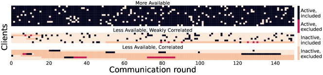
Figure 1: Clients’ activities and CA-Fed’s clients selection on the synthetic dataset.

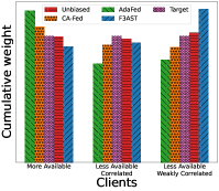
Figure 2: Importance given to the clients by the different algorithms throughout a whole training process on the synthetic dataset.

V-A Experimental Setup

Federated system simulator

In our experiments, we simulate the clients’ availability dynamics featuring different levels of temporal correlations. We model the activity of each client as a two-state homogeneous Markov process with state space $\mathcal{S}=\{\text{``\emph{active}''},\text{``\emph{inactive}''}\}$. We use $p_{k,s}$ to denote the probability that client $k\in\mathcal{K}$ remains in state $s\in\mathcal{S}$.

In order to simulate the statistical heterogeneity present in the federated learning system, we consider an experimental setting with two disjoint groups of clients ${G}_{i},~{}i=1,2$, to which we associate two different data distributions $\mathcal{P}_{i},~{}i=1,2$, to be precised later. Let $r_{i}=|{G}_{i}|/N,~{}i=1,2$ denote the fraction of clients in group $i=1,2$. In order to simulate the heterogeneity of clients’ availability patterns in realistic federated systems, we split the clients of each group in two classes uniformly at random: “more available” clients whose steady-state probability to be active is ${\color[rgb]{0,0,0}\pi_{k,\text{active}}}=1/2+g$ and “less available” clients with ${\color[rgb]{0,0,0}\pi_{k,\text{active}}}=1/2-g$, where $g\in(0,1/2)$ is a parameter controlling the heterogeneity of clients availability. We furthermore split each class of clients in two sub-classes uniformly at random: “correlated” clients that tend to persist in the same state (${\color[rgb]{0,0,0}\lambda_{k}}=\nu$ with values of $\nu$ close to $1$), and “weakly correlated” clients that are almost as likely to keep as to change their state (${\color[rgb]{0,0,0}\lambda_{k}}\sim\mathcal{N}(0,\varepsilon^{2})$, with $\varepsilon$ close to $0$). In our experiments, we suppose that $r_{1}=r_{2}=1/2$, $g=0.4$, $\nu=0.9$, and $\varepsilon=10^{-2}$.

Datasets and models

All experiments are performed on a binary classification synthetic dataset (described in Appendix -F) and on the real-world MNIST dataset [35], using $N=24$ clients. For MNIST dataset, we introduce statistical heterogeneity across the two groups of clients (i.e., we make the two distributions $\mathcal{P}_{1}$ and $\mathcal{P}_{2}$ different), following the same approach in [36]: 1) every client is assigned a random subset of the total training data; 2) the data of clients from the second group is modified by randomly swapping two pairs of labels. We maintain the original training/test data split of MNIST and use $20\%$ of the training dataset as validation dataset. We use a linear classifier with a ridge penalization of parameter $10^{-2}$, which is a strongly convex objective function, for both the synthetic and the real-world MNIST datasets.

Benchmarks

We compare CA-Fed, defined in Algorithm 1, with the Unbiased aggregation strategy, where all the active clients participate and receive a weight inversely proportional to their availability, and with the state-of-the-art FL algorithms discussed in Section II: F3AST [18] and AdaFed [19]. We tuned the learning rates $\eta,~{}\eta_{s}$ via grid search, on the grid $\eta:\{10^{-3},10^{-2.5},10^{-2},10^{-1.5},10^{-1}\}$, $\eta_{s}:\{10^{-2},10^{-1.5},10^{-1},10^{-0.5},10^{0}\}$. For CA-Fed, we used $\tau=0$, $\beta=0.2$. We assume all algorithms can access an oracle providing the true availability parameters for each client. In practice, Unbiased, AdaFed, and F3AST rely on the exact knowledge of ${\color[rgb]{0,0,0}\pi_{k,\text{active}}}$, and CA-Fed on ${\color[rgb]{0,0,0}\pi_{k,\text{active}}}$ and ${\color[rgb]{0,0,0}\lambda_{k}}$.

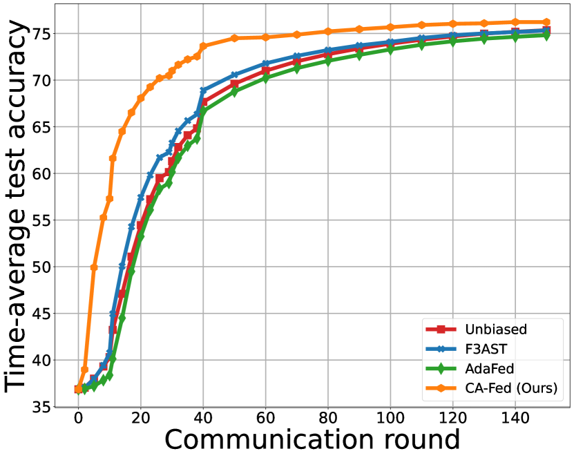
(a) Synthetic

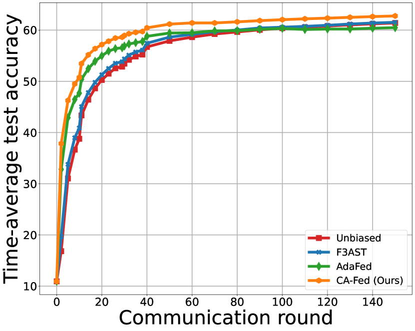
(b) MNIST

Figure 3: Test accuracy vs number of communication rounds.

V-B Experimental Results

Figure 1 shows the availability of each client during a training run on the synthetic dataset. Clients selected (resp. excluded) by CA-Fed are highlighted in black (resp. red). We observe that excluded clients tend to be those with low average availability or high correlation.

Figure 2 shows the importance $p_{k}$ (averaged over time) given by different algorithms to each client $k$ during a full training run. We observe that all the algorithms, except Unbiased, depart from the target importance $\bm{\alpha}$. As suggested by guidelines A and B, CA-Fed tends to favor the group of “more available” clients, at the expense of the “less available” clients.

Figure 3 shows the time-average accuracy up to round $t$ of the learned model averaged over three different runs. On both datasets, CA-Fed achieves the highest accuracy, which is about a percentage point higher than the second best algorithm (F3AST). Table I shows for each algorithm: the average over three runs of the maximum test accuracy achieved during training, the time-average test accuracy achieved during training, together with its standard deviation within the second half of the training period. Results show that while CA-Fed achieves a maximum accuracy which is comparable to the Unbiased baseline and state-of-the-art AdaFed and F3AST, it gets a higher time-average accuracy ($1.24$ percentage points) in comparison to the second best (F3AST), and a smaller standard deviation ($1.5\times$) in comparison to the second best (F3AST).

TABLE I: Maximum and time-average test accuracy, together with their standard deviations, on the Synthetic / MNIST datasets.

	Test Accuracy
	Maximum	Time-average	Standard deviation
Unbiased	$78.94$ $\,/\,$ $64.87$	$75.32$ $\,/\,$ $61.39$	$0.48$ $\,/\,$ $1.09$
F3AST	$78.97$ $\,/\,$ $64.91$	$75.33$ $\,/\,$ $61.52$	$0.40$ $\,/\,$ $0.94$
AdaFed	$78.69$ $\,/\,$ $63.77$	$74.81$ $\,/\,$ $60.48$	$0.59$ $\,/\,$ $1.37$
CA-Fed	$\bm{79.03}$ $\,/\,$ $\bm{64.94}$	$\bm{76.22}$ $\,/\,$ $\bm{62.76}$	$\bm{0.28}$ $\,/\,$ $\bm{0.61}$

VI Discussion

In this section, we discuss some general concerns and remarks on our algorithm.

VI-A Controlling the number of excluded clients

Theorems 1 and 3 suggest that the condition number $\kappa^{2}$ can play a meaningful role in the minimization of the total error $\epsilon$. Our algorithm uses a proxy ($\epsilon^{(t)}$) of the total error. To take into account the effect of $\kappa^{2}$, we can introduce a hyper-parameter that weights the relative importance of the optimization and bias error in (14):

$${\epsilon^{\prime}}^{(t)}\coloneqq F_{B}(\bm{w}_{t,0})-F_{B}^{*}+\bar{\kappa}^{2}\cdot d_{TV}^{2}(\bm{\alpha},\bm{p})\Gamma^{\prime}.$$

A small value of $\bar{\kappa}^{2}$ penalizes the bias term in favor of the optimization error, resulting in a larger number of clients excluded by CA-Fed. On the other hand, CA-Fed tends to include more clients for a large value of $\bar{\kappa}^{2}$. Asymptotically, for $\bar{\kappa}^{2}\rightarrow+\infty$, CA-Fed reduces to the Unbiased baseline. To further improve the performance of CA-Fed, a finer tuning of the values of $\bar{\kappa}^{2}$ can be performed.

VI-B CA-Fed in presence of spatial correlation

Although CA-Fed is mainly designed to handle temporal correlation, it does not necessarily perform poorly in presence of spatial correlation, as well.

Consider the following spatially-correlated scenario: clients are grouped in clusters, each cluster $c\in\mathcal{C}$ is characterized by an underlying Markov chain, which determines when all clients in the cluster are available/unavailable, the Markov chains of different clusters are independent. Let $\lambda_{c}$ denote the second largest eigenvalue in module of cluster-$c$’s Markov chain. In this case, one needs to exclude all clients in the cluster $\bar{c}=\arg\max_{c\in\mathcal{C}}\lambda_{c}$ to reduce the eigenvalue of the aggregate Markov chain.

In this setting, CA-Fed would associate similar eigenvalue estimates to all clients in the same cluster, then it would correctly start considering for exclusion the clients in cluster $\bar{c}$ and potentially remove sequentially all clients in the same cluster. These considerations suggest that CA-Fed may still operate correctly even in presence of spatial correlation.

VI-C About CA-Fed’s fairness

A strategy that excludes clients from the training phase, such as CA-Fed, may naturally raise fairness concerns. The concept of fairness in FL does not have a unified definition in the literature [37, Chapter 8]: fairness goals can be captured by a suitable choice of the target weights in (1). For example, per-client fairness can be achieved by setting $\alpha_{k}$ equal for every client, while per-sample fairness by setting $\alpha_{k}$ proportional to the local dataset size $|D_{k}|$. If we assume that the global objective in (1) indeed reflects also fairness concerns, then CA-Fed is intrinsically fair, in the sense that it guarantees that the performance objective of the learned model is as close as possible to its minimum value.

VII Conclusion

This paper presented the first convergence analysis for a FedAvg-like FL algorithm under heterogeneous and correlated client availability. The analysis quantifies how correlation adversely affects the algorithm’s convergence rate and highlights a general bias-versus-convergence-speed trade-off. Guided by the theoretical analysis, we proposed CA-Fed, a new FL algorithm that tries to balance the conflicting goals of maximizing convergence speed and minimizing model bias. Our experimental results demonstrate that adaptively excluding clients with high temporal correlation and low availability is an effective approach to handle the heterogeneous and correlated client availability in FL.

-A Proof of Theorem 1

We bound the optimization error of the target objective as the optimization error of the biased objective plus a bias term:

$$\textstyle F(\bm{w})-F^{*} \textstyle\stackrel{{\scriptstyle\text{\tiny(a)}}}{{\leq}}\frac{1}{2\mu}\left\lVert\nabla F(\bm{w})\right\rVert^{2}\stackrel{{\scriptstyle\text{\tiny(b)}}}{{\leq}}\frac{L^{2}}{2\mu}\left\lVert\bm{w}-\bm{w}^{*}\right\rVert^{2}$$

$$\textstyle\stackrel{{\scriptstyle\text{\tiny(c)}}}{{\leq}}\frac{L^{2}}{\mu}(\left\lVert\bm{w}-\bm{w}_{B}^{*}\right\rVert^{2}+\left\lVert\bm{w}_{B}^{*}-\bm{w}^{*}\right\rVert^{2})$$

$$\textstyle\stackrel{{\scriptstyle\text{\tiny(d)}}}{{\leq}}\underbrace{\textstyle\frac{2L^{2}}{\mu^{2}}(F_{B}(\bm{w})-F_{B}^{*})}_{\coloneqq\epsilon_{\text{opt}}}+\underbrace{\textstyle\frac{2L^{2}}{\mu^{2}}(F(\bm{w}_{B}^{*})-F^{*})}_{\coloneqq\epsilon_{\text{bias}}},$$

where $(a)$, $(b)$, and $(d)$ follow from the Assumptions 3, 4, and the inequality $(c)$ follows from $(a+b)^{2}\leq 2a^{2}+2b^{2}$. In particular, $(b)$ requires $\nabla F_{k}(\bm{w}_{k}^{*})=0$. Theorem 2 further develops the optimization error $\epsilon_{\text{opt}}$. We now expand $\epsilon_{\text{bias}}$:

$$\textstyle\left\lVert\nabla F(\bm{w}_{B}^{*})\right\rVert \textstyle\stackrel{{\scriptstyle\text{\tiny(e)}}}{{=}}\left\lVert\sum_{k=1}^{N}(\alpha_{k}-p_{k})\nabla F_{k}(\bm{w}_{B}^{*})\right\rVert$$

$$\textstyle\stackrel{{\scriptstyle\text{\tiny(f)}}}{{\leq}}L\sum_{k=1}^{N}\lvert\alpha_{k}-p_{k}\rvert\left\lVert\bm{w}_{B}^{*}-\bm{w}_{k}^{*}\right\rVert$$ (19)

$$\textstyle\stackrel{{\scriptstyle\text{\tiny(g)}}}{{\leq}}L\sqrt{\frac{2}{\mu}}\sum_{k=1}^{N}\frac{\lvert\alpha_{k}-p_{k}\rvert}{\sqrt{p_{k}}}\sqrt{p_{k}(F_{k}(\bm{w}_{B}^{*})-F_{k}^{*})},$$

where $(e)$ uses $\nabla F_{B}(\bm{w}_{B}^{*})=0$; $(f)$ applies first the triangle inequality, then the $L$-smoothness, and $(g)$ follows from the $\mu$-strong convexity. In addition, $(f)$ requires $\nabla F_{k}(\bm{w}_{k}^{*})=0$. Similarly to [32], in $(g)$ we multiply numerator and denominator by $\sqrt{p_{k}}$. By direct calculations, it follows that:

$$\textstyle\left\lVert\nabla F(\bm{w}_{B}^{*})\right\rVert^{2} \textstyle\stackrel{{\scriptstyle\text{\tiny(h)}}}{{\leq}}\frac{2L^{2}}{\mu}\Big{(}\sum_{k=1}^{N}{\frac{\lvert\alpha_{k}-p_{k}\rvert}{\sqrt{p_{k}}}}\sqrt{p_{k}(F_{k}(\bm{w}_{B}^{*})-F_{k}^{*})}\Big{)}^{2}$$

$$\textstyle\stackrel{{\scriptstyle\text{\tiny(i)}}}{{\leq}}\frac{2L^{2}}{\mu}\Big{(}\sum\limits_{\scriptscriptstyle k=1}^{\scriptscriptstyle N}\frac{(\alpha_{k}-p_{k})^{2}}{p_{k}}\Big{)}\Big{(}\sum\limits_{\scriptscriptstyle k=1}^{\scriptscriptstyle N}p_{k}(F_{k}(\bm{w}_{B}^{*})-F_{k}^{*})\Big{)}$$

$$\textstyle\stackrel{{\scriptstyle\text{\tiny(j)}}}{{\leq}}\frac{2L^{2}}{\mu}\chi^{2}_{\bm{\alpha}\parallel\bm{p}}\Gamma,$$

where $(i)$ uses the Cauchy–Schwarz inequality, and $(j)$ used:

$$\textstyle\sum_{k=1}^{N}p_{k}(F_{k}(\bm{w}_{B}^{*})-F_{k}^{*})\leq\sum_{k=1}^{N}p_{k}(F_{k}(\bm{w}^{*})-F_{k}^{*})\leq\Gamma.$$

Finally, by strong convexity of $F$, we conclude that:

$$\textstyle F(\bm{w}_{B}^{*})-F^{*}\leq\frac{1}{2\mu}\left\lVert\nabla F(\bm{w}_{B}^{*})\right\rVert^{2}\leq\frac{L^{2}}{\mu^{2}}\chi^{2}_{\bm{\alpha}\parallel\bm{p}}\Gamma.\qed$$

-B Proof of Theorem 2

-B1 Additional notation

let $\bm{w}_{t,j}^{k}$ be the model parameter vector computed by device $k$ at the global round $t$, local iteration $j$. We define:

$$\textstyle g_{t}(A_{t})=\sum_{k\in A_{t}}q_{k}\sum_{j=0}^{E-1}\nabla F_{k}(\bm{w}_{t,j}^{k},\xi_{t,j}^{k}),$$

and $\bar{g}_{t}(A_{t})=\operatorname*{\mathbb{E}}\nolimits_{\xi|A_{t}}[g_{t}(A_{t})].$

Following (2) and (3), the update rule of CA-Fed is:

$$\bm{w}_{t+1,0}=\mathbf{Proj}_{W}{(\bm{w}_{t,0}-\eta_{t}g_{t}(A_{t}))}.$$ (20)

-B2 Key lemmas and results

we provide useful lemmas and results to support the proof of the main theorem.

Proof of Lemma 1. The boundedness of $W$ gives a bound on $({\bm{w}}_{t,0})_{t\geq 0}$ based on the update rules in (2) and (3). From the convexity of $\{F_{k}\}_{k\in\mathcal{K}}$, it follows that:

$$D\coloneqq\sup_{\bm{w}\in W,k\in\mathcal{K}}\|\nabla F_{k}(\bm{w})\|<+\infty.$$

Items (6), (8) are directly derived from the previous observation. Item (7) follows combining (6) and Assumption 5:

$$\textstyle\operatorname*{\mathbb{E}}\|\nabla F_{k}(\bm{w},\xi)\|^{2}\leq D^{2}+\max\limits_{\scriptscriptstyle k\in\mathcal{K}}\{\sigma_{k}^{2}\}\coloneqq G^{2}.\qed$$

Lemma 2 (Convergence under heterogeneous client availability).

Let the local functions $\{F_{k}\}_{k\in\mathcal{K}}$ be convex, Assumptions 3, 5 hold. If $\eta_{t}\leq\frac{1}{2L(EQ+1)}$, we have:

$$\textstyle\sum_{t}\eta_{t} \textstyle\operatorname*{\mathbb{E}}[\sum_{k\in A_{t}}q_{k}\left(F_{k}(\bm{w}_{t,0})-F_{k}(\bm{w}_{B}^{*})\right)]\leq$$

$$\textstyle+\frac{2}{E}\left\lVert\bm{w}_{0,0}-\bm{w}_{B}^{*}\right\rVert^{2}+2\sum_{k=1}^{N}\pi_{k}q_{k}^{2}\sigma_{k}^{2}\sum_{t}\eta_{t}^{2}$$

$$\textstyle+\frac{2}{3}\sum_{k=1}^{N}\pi_{k}q_{k}(E-1)(2E-1)G^{2}\sum_{t}\eta_{t}^{2}$$

$$\textstyle+2L(EQ+2)\sum_{k=1}^{N}\pi_{k}q_{k}\Gamma\sum_{t}\eta_{t}^{2}:=C_{1}<+\infty.$$

Proof of Lemma 2.

$$\left\lVert\bm{w}_{t+1,0}-\bm{w}_{B}^{*}\right\rVert^{2}=\left\lVert\mathbf{Proj}_{W}{(\bm{w}_{t,0}-\eta_{t}g_{t})}-\mathbf{Proj}_{W}{(\bm{w}_{B}^{*})}\right\rVert^{2}$$

$$\leq\left\lVert\bm{w}_{t,0}-\eta_{t}g_{t}-\bm{w}_{B}^{*}+\eta_{t}\bar{g}_{t}-\eta_{t}\bar{g}_{t}\right\rVert^{2}=A_{1}+A_{2}+A_{3},$$

where:

$$A_{1} =\left\lVert\bm{w}_{t,0}-\bm{w}_{B}^{*}-\eta_{t}\bar{g}_{t}\right\rVert^{2},$$

$$A_{2} =2\eta_{t}\langle\bm{\bm{w}}_{t,0}-\bm{w}_{B}^{*}-\eta_{t}\bar{g}_{t},\bar{g}_{t}-g_{t}\rangle,$$

$$A_{3} =\eta_{t}^{2}\left\lVert g_{t}-\bar{g}_{t}\right\rVert^{2}.$$

Note $\operatorname*{\mathbb{E}}[A_{2}]=0$. We bound $A_{1}$, $A_{3}$ using the key steps in [22]:

(1) the variance of $g_{t}(A_{t})$ is bounded if the variance of the stochastic gradients at each device is bounded:

$$A_{3} \textstyle=\operatorname*{\mathbb{E}}_{\mathcal{B}\mid A_{t}}\left\lVert g_{t}-\bar{g}_{t}\right\rVert^{2}=$$

$$\textstyle=\sum_{k\in A_{t}}q_{k}^{2}\sum_{j=0}^{E-1}\operatorname*{\mathbb{E}}_{\mathcal{B}\mid A_{t}}\left\lVert\nabla F_{k}(\bm{w}_{t,j}^{k},\xi_{t,j}^{k}){-}\nabla F_{k}(\bm{w}_{t,j}^{k})\right\rVert^{2}$$

$$\textstyle\leq E\sum_{k\in A_{t}}q_{k}^{2}\sigma_{k}^{2};$$

(2) the distance of the local model $\bm{w}_{t,E}^{k}$ from the global model $\bm{w}_{t,0}$ is bounded since the expected squared norm of the stochastic gradients is bounded:

$$\textstyle\operatorname*{\mathbb{E}}_{\mathcal{B}\mid A_{t}}\sum_{k\in A_{t}}q_{k}\sum_{j=0}^{E-1}\left\lVert\bm{w}_{t,j}^{k}-\bm{w}_{t,0}\right\rVert^{2}=$$

$$\textstyle\quad=\operatorname*{\mathbb{E}}_{\mathcal{B}\mid A_{t}}\sum_{k\in A_{t}}q_{k}\sum_{j=1}^{E-1}\eta_{t}^{2}\left\lVert\sum_{j^{\prime}=0}^{j-1}\nabla F_{k}(\bm{w}_{t,j^{\prime}}^{k},\xi_{t,j^{\prime}}^{k})\right\rVert^{2}$$

$$\textstyle\quad\leq\eta_{t}^{2}\sum_{k\in A_{t}}q_{k}\sum_{j=1}^{E-1}j\sum_{j^{\prime}=0}^{j-1}\operatorname*{\mathbb{E}}_{\mathcal{B}\mid A_{t}}\left\lVert\nabla F_{k}(\bm{w}_{t,j^{\prime}}^{k},\xi_{t,j^{\prime}}^{k})\right\rVert^{2}$$

$$\textstyle\quad\leq\eta_{t}^{2}\sum_{k\in A_{t}}q_{k}G^{2}\sum_{j=1}^{E-1}j^{2}$$

$$\textstyle\quad=\frac{1}{6}\eta_{t}^{2}\sum_{k\in A_{t}}q_{k}E(E-1)(2E-1)G^{2}.\qed$$

Lemma 3 (Optimization error after $\mathcal{J}_{t}$ steps).

Let Assumptions 1, 2 hold, the local functions $\{F_{k}\}_{k\in\mathcal{K}}$ be convex, $D,H$ be defined as in (6), (8), and $\mathcal{J}_{t}$ defined as in Theorem 2. Then:

$$\textstyle\sum_{t}\textstyle\eta_{t}\operatorname*{\mathbb{E}}[\sum_{k\in A_{t}}q_{k}(F_{k}(\bm{w}_{t-\mathcal{J}_{t},0})-F_{k}(\bm{w}_{t,0}))]$$

$$\textstyle\leq EDGQ\sum_{t}\mathcal{J}_{t}\eta_{t-\mathcal{J}_{t}}^{2}\sum_{k=1}^{N}\pi_{k}q_{k}:=\frac{C_{3}}{\ln(1/\lambda(\bm{P}))}<+\infty.$$

For the proof of Lemma 3, we introduce the following results:

$$\textstyle\lvert F_{k}(\bm{v})-F_{k}(\bm{w})\rvert\leq D\cdot\left\lVert\bm{v}-\bm{w}\right\rVert,~{}\forall\bm{v},\bm{w}\in W,$$ (21)

$$\textstyle\operatorname*{\mathbb{E}}_{{\color[rgb]{0,0,0}\mathcal{B}_{t,0}^{k}},\dots,{\color[rgb]{0,0,0}\mathcal{B}^{k}_{t,E{-}1}}}\left\lVert\bm{w}_{t+1,0}-\bm{w}_{t,0}\right\rVert\leq\eta_{t}GE(\sum_{k\in A_{t}}q_{k}).$$ (22)

Equation (21) is due to convexity of $\{F_{k}\}_{k\in\mathcal{K}}$, which gives:

$$\textstyle\langle\nabla F_{k}(\bm{v}),\bm{v}-\bm{w}\rangle\leq\left\lVert F_{k}(\bm{v})-F_{k}(\bm{w})\right\rVert\leq\langle\nabla F_{k}(\bm{w}),\bm{v}-\bm{w}\rangle;$$

the Cauchy–Schwarz inequality concludes:

$$\textstyle\lvert F_{k}(\bm{v})-F_{k}(\bm{w})\rvert \leq\max\{\left\lVert\nabla F_{k}(\bm{v})\right\rVert,\left\lVert\nabla F_{k}(\bm{w})\right\rVert\}\left\lVert\bm{v}-\bm{w}\right\rVert$$

$$\leq D\cdot\left\lVert\bm{v}-\bm{w}\right\rVert.$$

Equation (22) follows combining equations (7) and (20):

$$\textstyle\operatorname*{\mathbb{E}}_{\mathcal{B}|A_{t}} \left\lVert\bm{w}_{t+1,0}-\bm{w}_{t,0}\right\rVert\leq$$

$$\textstyle\leq\eta_{t}\operatorname*{\mathbb{E}}_{\mathcal{B}|A_{t}}\left\lVert\sum_{k\in A_{t}}q_{k}\sum_{j=0}^{E-1}\nabla F_{k}(\bm{w}_{t,j}^{k},\xi_{t,j}^{k})\right\rVert$$

$$\textstyle\leq\eta_{t}\sum_{k\in A_{t}}q_{k}\sum_{j=0}^{E-1}\operatorname*{\mathbb{E}}_{\mathcal{B}|A_{t}}\left\lVert\nabla F_{k}(\bm{w}_{t,j}^{k},\xi_{t,j}^{k})\right\rVert$$

$$\textstyle\leq\eta_{t}GE(\sum_{k\in A_{t}}q_{k}).$$

Proof of Lemma 3.

The evolution of the local objectives after $\mathcal{J}_{t}$ communication rounds is bounded:

$$\textstyle\sum_{t} \textstyle\eta_{t}\operatorname*{\mathbb{E}}[\sum_{k\in A_{t}}q_{k}(F_{k}(\bm{w}_{t-\mathcal{J}_{t},0})-F_{k}(\bm{w}_{t,0}))]$$

$$\textstyle\stackrel{{\scriptstyle\text{\tiny(a)}}}{{\leq}}D\sum_{t}\eta_{t}\operatorname*{\mathbb{E}}[\sum_{k\in A_{t}}q_{k}\operatorname*{\mathbb{E}}_{B}\left\lVert\bm{w}_{t-\mathcal{J}_{t},0}-\bm{w}_{t,0}\right\rVert]$$

$$\textstyle\stackrel{{\scriptstyle\text{\tiny(b)}}}{{\leq}}D\sum_{t}\eta_{t}\sum_{d=t-\mathcal{J}_{t}}^{t-1}\operatorname*{\mathbb{E}}[\sum_{k\in A_{t}}q_{k}\operatorname*{\mathbb{E}}_{B}\left\lVert\bm{w}_{d,0}-\bm{w}_{d+1,0}\right\rVert]$$

$$\textstyle\stackrel{{\scriptstyle\text{\tiny(c)}}}{{\leq}}EDG\sum_{t}\sum_{d=t-\mathcal{J}_{t}}^{t-1}\eta_{t}\eta_{d}\operatorname*{\mathbb{E}}[\sum_{k\in A_{t}}q_{k}\sum_{k^{\prime}\in A_{d}}q_{k^{\prime}}]$$

$$\textstyle\stackrel{{\scriptstyle\text{\tiny(d)}}}{{\leq}}\frac{EDG}{2}\sum_{t}\sum_{d=t-\mathcal{J}_{t}}^{t-1}(\eta_{t}^{2}+\eta_{d}^{2})\operatorname*{\mathbb{E}}[\sum_{k\in A_{t}}q_{k}\sum_{k^{\prime}\in A_{d}}q_{k^{\prime}}]$$

$$\textstyle\stackrel{{\scriptstyle\text{\tiny(e)}}}{{\leq}}EDGQ\sum_{t}\mathcal{J}_{t}\eta_{t-\mathcal{J}_{t}}^{2}\sum_{k=1}^{N}\pi_{k}q_{k}:=\frac{C_{3}}{\ln(1/\lambda(\bm{P}))},$$

where $(a)$ follows from (21); $(b)$ applies the triangle inequality; $(c)$ uses (22); $(d)$ applies the Cauchy–Schwarz inequality; $(e)$ uses $\eta_{t}<\eta_{d}\leq\eta_{t-\mathcal{J}_{t}}$ and $\sum_{k=1}^{N}q_{k}=Q$. ∎

-B3 Core of the proof

The proof consists in two main steps:

$1.\sum_{t}\eta_{t}\sum_{k=1}^{N}\pi_{k}q_{k}\operatorname*{\mathbb{E}}[F_{B}(\bm{w}_{t-\mathcal{J}_{t},0})-F_{B}^{*})]{\leq}C_{2}{+}\frac{C_{3}}{\ln(1/\lambda(\bm{P}))}$;

$2.\sum_{t}\eta_{t}\sum_{k=1}^{N}\pi_{k}q_{k}\operatorname*{\mathbb{E}}[F_{B}(\bm{w}_{t,0}){-}F_{B}(\bm{w}_{t-\mathcal{J}_{t},0})]{\leq}\frac{C_{3}}{\ln(1/\lambda(\bm{P}))}$.

Step 1. Combining Lemma 2 and 3, we get:

$$\textstyle\sum_{t}\eta_{t}\operatorname*{\mathbb{E}}[\sum\limits_{\scriptscriptstyle k\in A_{t}}q_{k}(F_{k}(\bm{w}_{t-\mathcal{J}_{t},0})-F_{k}(\bm{w}_{B}^{*}))]\leq C_{1}+\frac{C_{3}}{\ln(1/\lambda(\bm{P}))}.$$

The constant $\mathcal{J}_{t}$, introduced in [14], is an important parameter for the analysis and frequently used. Combining its definition in Theorem 2 and equation (5), it follows:

$$\textstyle\left\lvert[P^{\mathcal{J}_{t}}]_{i,j}-\pi_{j}\right\rvert\leq C_{P}\lambda(\bm{P})^{\mathcal{J}_{t}}\leq\frac{1}{2Ht},\quad\forall i,j\in[M].$$ (23)

Assume $t\geq T_{P}$. We derive an important lower bound:

$$\textstyle\operatorname*{\mathbb{E}}_{A_{t}\mid A_{t-\mathcal{J}_{t}}}[\sum_{k\in A_{t}}q_{k}(F_{k}(\bm{w}_{t-\mathcal{J}_{t},0})-F_{k}(\bm{w}_{B}^{*}))]$$

$$\textstyle\stackrel{{\scriptstyle\text{\tiny(a)}}}{{=}}\sum_{\mathcal{I}=1}^{M}\mathbb{P}(A_{t}{=}\mathcal{I}{\mid}A_{t-\mathcal{J}_{t}})\sum_{k\in\mathcal{I}}q_{k}(F_{k}(\bm{w}_{t-\mathcal{J}_{t},0}){-}F_{k}(\bm{w}_{B}^{*}))$$

$$\textstyle\stackrel{{\scriptstyle\text{\tiny(b)}}}{{=}}\sum_{\mathcal{I}=1}^{M}~{}[P^{\mathcal{J}_{t}}]_{A_{t-\mathcal{J}_{t}},\mathcal{I}}~{}\sum_{k\in\mathcal{I}}q_{k}\left(F_{k}(\bm{w}_{t-\mathcal{J}_{t},0})-F_{k}(\bm{w}_{B}^{*})\right)$$

$$\textstyle\stackrel{{\scriptstyle\text{\tiny(c)}}}{{\geq}}\sum_{\mathcal{I}=1}^{M}~{}\left(\pi(\mathcal{I})-\frac{1}{2Ht}\right)\sum_{k\in\mathcal{I}}q_{k}(F_{k}(\bm{w}_{t-\mathcal{J}_{t},0})-F_{k}(\bm{w}_{B}^{*}))$$

$$\textstyle\stackrel{{\scriptstyle\text{\tiny(d)}}}{{\geq}}(\sum_{k=1}^{N}\pi_{k}q_{k})\cdot(F_{B}(\bm{w}_{t-\mathcal{J}_{t},0})-F_{B}^{*})-\frac{1}{2t}MQ,$$ (24)

where $(a)$ is the definition of the conditional expectation, $(b)$ uses the Markov property, $(c)$ follows from (23), and $(d)$ is due to (8). Taking total expectations:

$$\textstyle( \textstyle\sum_{k=1}^{N}\pi_{k}q_{k})\sum_{t}\eta_{t}\operatorname*{\mathbb{E}}[F_{B}(\bm{w}_{t-\mathcal{J}_{t},0})-F_{B}^{*}]$$

$$\textstyle\leq\sum_{t}\eta_{t}\operatorname*{\mathbb{E}}[\sum_{k\in A_{t}}q_{k}(F_{k}(\bm{w}_{t-\mathcal{J}_{t},0})-F_{k}(\bm{w}_{B}^{*}))]$$

$$\textstyle\quad+\frac{1}{4}MQ\sum_{t}(\eta_{t}^{2}+\frac{1}{t^{2}})=C_{2}+\frac{C_{3}}{\ln(1/\lambda(\bm{P}))},$$ (25)

where $C_{2}=C_{1}+\frac{1}{4}MQ\sum_{t}(\eta_{t}^{2}+\frac{1}{t^{2}})$.

Step 2. By direct calculation (similar to Lemma 3):

$$\textstyle(\sum_{k=1}^{N}\pi_{k}q_{k})\sum_{t}\eta_{t}\operatorname*{\mathbb{E}}[F_{B}(\bm{w}_{t,0})-F_{B}(\bm{w}_{t-\mathcal{J}_{t},0})]{\leq}\frac{C_{3}}{\ln(1/\lambda(\bm{P}))}.$$

Summing Step 1 and 2, and applying Jensen’s inequality:

$$\textstyle(\sum_{t=1}^{T}\eta_{t})(\sum_{k=1}^{N}\pi_{k}q_{k})\operatorname*{\mathbb{E}}[F_{B}(\bar{\bm{w}}_{T,0})-F_{B}^{*}]\leq$$

$$\textstyle(\sum_{k=1}^{N}\pi_{k}q_{k})\sum_{t=1}^{T}\eta_{t}\operatorname*{\mathbb{E}}[F_{B}(\bm{w}_{t,0})-F_{B}^{*}]\leq C_{2}+\frac{2C_{3}}{\ln(1/\lambda(\bm{P}))},$$

where $\bar{\bm{w}}_{T,0}:=\frac{\sum_{t=1}^{T}\eta_{t}\bm{w}_{t,0}}{\sum_{t=1}^{T}\eta_{t}}$, and the constants are in (12). ∎

-C Proof of Theorem 3

It follows the same lines of Theorem 1, developing (19) as:

$$\textstyle\left\lVert\nabla F(\bm{w}_{B}^{*})\right\rVert \textstyle\leq L\sqrt{\frac{2}{\mu}}\sum_{k=1}^{N}\lvert\alpha_{k}-p_{k}\rvert\sqrt{(F_{k}(\bm{w}_{B}^{*})-F_{k}^{*})}$$

$$\textstyle\leq 2L\sqrt{\frac{2}{\mu}}d_{TV}(\bm{\alpha},\bm{p})\sqrt{{\Gamma}^{\prime}},$$

where $d_{TV}(\bm{\alpha},\bm{p})\coloneqq\frac{1}{2}\sum_{k=1}^{N}\lvert\alpha_{k}-p_{k}\rvert$ is the total variation distance between the probability measures $\bm{\alpha}$ and $\bm{p}$. ∎

-D Minimizing $\epsilon_{\text{opt}}$

Equation 12 defines the following optimization problem: qf(q)=12q⊺A q + Bπ⊺q + C;  q ≥0  π^⊺q ¿ 0 ∥q∥1 = Q. Let us rewrite the problem by adding a variable $s:=1/\bm{\pi}^{\intercal}\bm{q}$ and then replacing $\bm{y}:=s\bm{q}$. Note that the objective function is the perspective of a convex function, and is therefore convex: —s— y,s f(y,s) = 12s y⊺A y + Bs + C y ≥0,  s ¿ 0,  π^⊺y = 1,  ∥y∥_1=Qs. The Lagrangian function $\mathcal{L}$ is as follows:

$$\mathcal{L}(\bm{y},s,\lambda,\theta,\bm{\mu})=\textstyle\frac{1}{2s}\bm{y}^{\intercal}\bm{A}\bm{y}+Bs+C+$$

$$+\lambda(1-\bm{\pi}^{\intercal}\bm{y})+\theta(\textstyle{\left\lVert\bm{y}\right\rVert_{1}-Qs)}-\bm{\mu}^{\intercal}\bm{y}.$$ (26)

Since the constraint $s>0$ defines an open set, the set defined by the constraints in (-D) is not closed. However, the solution is never on the boundary $s=0$ because $\mathcal{L}^{*}\rightarrow+\infty$ as $s\rightarrow 0^{+}$, and we can consider $s\geq 0$. The KKT conditions for $y_{k}^{*}$ read:

$$\textstyle\text{if $y_{k}^{*}>0$:}~{}y_{k}^{*}=\frac{s^{*}}{A[{kk}]}(\lambda^{*}\pi_{k}-\theta^{*});\hfill~{}\text{$y_{k}^{*}=0$ otherwise.}$$ (27)

Since $\lambda^{*}\geq 0$, the clients with smaller $\pi_{k}$ may have $q_{k}^{*}=0$.

-E Convexity of $\epsilon_{\text{opt}}+\epsilon_{\text{bias}}$

In Appendix -D, we proved that $\epsilon_{\text{opt}}(\bm{q})$ is convex. To prove that $\epsilon_{\text{bias}}(\bm{q})$ is also convex, we need to study the convexity of $\chi^{2}_{\bm{\alpha}\parallel\bm{p}}=\sum_{\scriptscriptstyle k=1}^{\scriptscriptstyle N}(f_{k}\circ g_{k})(\bm{q})$, where $f_{k}(p_{k})=(p_{k}-\alpha_{k})^{2}/p_{k}$, and $g_{k}(\bm{q})=(\pi_{k}q_{k})/\sum_{\scriptscriptstyle h=1}^{\scriptscriptstyle N}\pi_{h}q_{h}$. We observe that $f_{k}(p_{k})$ is convex, and $g_{k}(\bm{q})$ is a particular case of linear-fractional function [38]. By direct inspection, it can be proved that $(f_{k}\circ g_{k})(\bm{q})$ is convex in $\text{dom}(f_{k}\circ g_{k})=\{\bm{q}:\left\lVert\bm{q}\right\rVert_{1}=Q>0\}$.

-F Synthetic dataset

Our synthetic datasets has been generated as follows:

1. For client $k\in\mathcal{K}$, sample group identity $i_{k}$ from a Bernoulli distribution of parameter $1/2$;

2. Sample model parameters $\bm{w}^{*}\sim\mathcal{N}(0,I_{d})$ from the $d$-dimensional normal distribution;

3. For client $k\in\mathcal{K}$ and sample index $j\in\{1,\dots,150\}$, sample clients input data $\bm{x}_{k}^{(j)}\sim\mathcal{N}(0,I_{d})$ from the $d$-dimensional normal distribution;

4. For client $k\in\mathcal{K}$ such that $i_{k}=0$ and sample index $j\in\{1,\dots,150\}$, sample the true labels $y_{k}^{(j)}$ from a Bernoulli distribution with parameter equal to $\text{sigmoid}(\langle\bm{w}^{*},\bm{x}_{k}^{(j)}\rangle)$;

5. For client $k\in\mathcal{K}$ such that $i_{k}=1$ and sample index $j\in\{1,\dots,150\}$, sample the true labels $y_{k}^{(j)}$ from a Bernoulli distribution with parameter equal to $0.8\cdot\text{sigmoid}(\langle\bm{w}^{*},\bm{x}_{k}^{(j)}\rangle)+0.2\cdot(1-\text{sigmoid}(\langle\bm{w}^{*},\bm{x}_{k}^{(j)}\rangle))$.

References

• [1] J. Verbraeken, M. Wolting, J. Katzy, J. Kloppenburg, T. Verbelen, and J. S. Rellermeyer, “A survey on distributed machine learning,” ACM Computing Surveys (CSUR), vol. 53, no. 2, pp. 1–33, 2020.
• [2] S. Wang, T. Tuor, T. Salonidis, K. K. Leung, C. Makaya, T. He, and K. Chan, “When edge meets learning: Adaptive control for resource-constrained distributed machine learning,” in IEEE INFOCOM 2018-IEEE Conference on Computer Communications.   IEEE, 2018, pp. 63–71.
• [3] J. Konečný, H. B. McMahan, F. X. Yu, P. Richtarik, A. T. Suresh, and D. Bacon, “Federated learning: Strategies for improving communication efficiency,” in NIPS Workshop on Private Multi-Party Machine Learning, 2016, https://arxiv.org/abs/1610.05492.
• [4] B. McMahan, E. Moore, D. Ramage, S. Hampson, and B. A. y Arcas, “Communication-efficient learning of deep networks from decentralized data,” in Artificial Intelligence and Statistics.   PMLR, 2017, pp. 1273–1282.
• [5] P. Kairouz, H. B. McMahan, B. Avent, A. Bellet, M. Bennis, A. N. Bhagoji, K. Bonawitz, Z. Charles, G. Cormode, R. Cummings et al., “Advances and open problems in federated learning,” Foundations and Trends® in Machine Learning, vol. 14, no. 1–2, pp. 1–210, 2021.
• [6] T. Li, A. K. Sahu, A. Talwalkar, and V. Smith, “Federated learning: Challenges, methods, and future directions,” IEEE Signal Processing Magazine, vol. 37, no. 3, pp. 50–60, 2020.
• [7] H. Eichner, T. Koren, B. McMahan, N. Srebro, and K. Talwar, “Semi-cyclic stochastic gradient descent,” in International Conference on Machine Learning.   PMLR, 2019, pp. 1764–1773.
• [8] J. Wang, Z. Charles, Z. Xu, G. Joshi, H. B. McMahan, M. Al-Shedivat, G. Andrew, S. Avestimehr, K. Daly, D. Data et al., “A field guide to federated optimization,” arXiv preprint arXiv:2107.06917, 2021.
• [9] K. Bonawitz, H. Eichner, W. Grieskamp, D. Huba, A. Ingerman, V. Ivanov, C. Kiddon, J. Konečnỳ, S. Mazzocchi, B. McMahan et al., “Towards federated learning at scale: System design,” Proceedings of Machine Learning and Systems, vol. 1, pp. 374–388, 2019.
• [10] Y. Ding, C. Niu, Y. Yan, Z. Zheng, F. Wu, G. Chen, S. Tang, and R. Jia, “Distributed optimization over block-cyclic data,” arXiv preprint arXiv:2002.07454, 2020.
• [11] C. Zhu, Z. Xu, M. Chen, J. Konečnỳ, A. Hard, and T. Goldstein, “Diurnal or Nocturnal? Federated Learning from Periodically Shifting Distributions,” in NeurIPS 2021 Workshop on Distribution Shifts: Connecting Methods and Applications, 2021.
• [12] T. T. Doan, “Local stochastic approximation: A unified view of federated learning and distributed multi-task reinforcement learning algorithms,” arXiv preprint arXiv:2006.13460, 2020.
• [13] T. T. Doan, L. M. Nguyen, N. H. Pham, and J. Romberg, “Convergence rates of accelerated Markov gradient descent with applications in reinforcement learning,” arXiv preprint arXiv:2002.02873, 2020.
• [14] T. Sun, Y. Sun, and W. Yin, “On Markov chain gradient descent,” Advances in neural information processing systems, vol. 31, 2018.
• [15] M. McCloskey and N. J. Cohen, “Catastrophic Interference in Connectionist Networks: The Sequential Learning Problem,” in Psychology of Learning and Motivation, G. H. Bower, Ed.   Academic Press, 1989, vol. 24, pp. 109–165.
• [16] J. Kirkpatrick, R. Pascanu, N. Rabinowitz, J. Veness, G. Desjardins, A. A. Rusu, K. Milan, J. Quan, T. Ramalho, A. Grabska-Barwinska et al., “Overcoming catastrophic forgetting in neural networks,” Proceedings of the National Academy of Sciences, vol. 114, no. 13, pp. 3521–3526, 2017.
• [17] M. Tang, X. Ning, Y. Wang, J. Sun, Y. Wang, H. Li, and Y. Chen, “FedCor: Correlation-Based Active Client Selection Strategy for Heterogeneous Federated Learning,” in Proceedings of the IEEE/CVF Conference on Computer Vision and Pattern Recognition, 2022.
• [18] M. Ribero, H. Vikalo, and G. De Veciana, “Federated Learning Under Intermittent Client Availability and Time-Varying Communication Constraints,” arXiv preprint arXiv:2205.06730, 2022.
• [19] L. Tan, X. Zhang, Y. Zhou, X. Che, M. Hu, X. Chen, and D. Wu, “AdaFed: Optimizing Participation-Aware Federated Learning with Adaptive Aggregation Weights,” IEEE Transactions on Network Science and Engineering, 2022.
• [20] A. Nichol, J. Achiam, and J. Schulman, “On first-order meta-learning algorithms,” arXiv preprint arXiv:1803.02999, 2018.
• [21] S. J. Reddi, Z. Charles, M. Zaheer, Z. Garrett, K. Rush, J. Konečný, S. Kumar, and H. B. McMahan, “Adaptive Federated Optimization,” in International Conference on Learning Representations, 2021.
• [22] X. Li, K. Huang, W. Yang, S. Wang, and Z. Zhang, “On the Convergence of FedAvg on Non-IID Data,” in International Conference on Learning Representations, 2019.
• [23] T. Li, A. K. Sahu, M. Zaheer, M. Sanjabi, A. Talwalkar, and V. Smith, “Federated optimization in heterogeneous networks,” Proceedings of Machine Learning and Systems, vol. 2, pp. 429–450, 2020.
• [24] W. Chen, S. Horvath, and P. Richtarik, “Optimal client sampling for federated learning,” arXiv preprint arXiv:2010.13723, 2020.
• [25] Y. Fraboni, R. Vidal, L. Kameni, and M. Lorenzi, “Clustered sampling: Low-variance and improved representativity for clients selection in federated learning,” in International Conference on Machine Learning.   PMLR, 2021, pp. 3407–3416.
• [26] Y. Jee Cho, J. Wang, and G. Joshi, “Towards Understanding Biased Client Selection in Federated Learning,” in Proceedings of The 25th International Conference on Artificial Intelligence and Statistics.   PMLR, 2022, pp. 10 351–10 375.
• [27] T. T. Doan, L. M. Nguyen, N. H. Pham, and J. Romberg, “Finite-time analysis of stochastic gradient descent under Markov randomness,” arXiv preprint arXiv:2003.10973, 2020.
• [28] A. Meyers and H. Yang, “Markov Chains for Fault-Tolerance Modeling of Stochastic Networks,” IEEE Transactions on Automation Science and Engineering, 2021.
• [29] H. Olle, P. Yuval, and E. S. Jeffrey, “Dynamical percolation,” in Annales de l’Institut Henri Poincare (B) Probability and Statistics, vol. 33, no. 4.   Elsevier, 1997, pp. 497–528.
• [30] D. A. Levin and Y. Peres, Markov chains and mixing times.   American Mathematical Soc., 2017, vol. 107.
• [31] L. Bottou, F. E. Curtis, and J. Nocedal, “Optimization methods for large-scale machine learning,” Siam Review, vol. 60, no. 2, pp. 223–311, 2018.
• [32] J. Wang, Q. Liu, H. Liang, G. Joshi, and H. V. Poor, “Tackling the objective inconsistency problem in heterogeneous federated optimization,” Advances in neural information processing systems, vol. 33, pp. 7611–7623, 2020.
• [33] I. J. Goodfellow, M. Mirza, D. Xiao, A. Courville, and Y. Bengio, “An empirical investigation of catastrophic forgetting in gradient-based neural networks,” in International Conference on Learning Representations, 2013, arXiv preprint arXiv:1312.6211.
• [34] R. Kemker, M. McClure, A. Abitino, T. Hayes, and C. Kanan, “Measuring catastrophic forgetting in neural networks,” in Proceedings of the AAAI Conference on Artificial Intelligence, vol. 32, no. 1, 2018.
• [35] Y. LeCun and C. Cortes, “MNIST handwritten digit database,” 2010.
• [36] F. Sattler, K.-R. Müller, and W. Samek, “Clustered federated learning: Model-agnostic distributed multitask optimization under privacy constraints,” IEEE Transactions on Neural Networks and Learning Systems, vol. 32, no. 8, pp. 3710–3722, 2020.
• [37] H. Ludwig and N. Baracaldo, Federated Learning: A Comprehensive Overview of Methods and Applications.   Springer Cham, 2022.
• [38] S. Boyd and L. Vandenberghe, Convex optimization.   Cambridge university press, 2004.