Discrete Elasticity Exact Sequences on Worsey-Farin splits

Abstract.

We construct conforming finite element elasticity complexes on Worsey-Farin splits in three dimensions. Spaces for displacement, strain, stress, and the load are connected in the elasticity complex through the differential operators representing deformation, incompatibility, and divergence. For each of these component spaces, a corresponding finite element space on Worsey-Farin meshes is exhibited. Unisolvent degrees of freedom are developed for these finite elements, which also yields commuting (cochain) projections on smooth functions. A distinctive feature of the spaces in these complexes is the lack of extrinsic supersmoothness at subsimplices of the mesh. Notably, the complex yields the first (strongly) symmetric stress finite element with no vertex or edge degrees of freedom in three dimensions. Moreover, the lowest order stress space uses only piecewise linear functions which is the lowest feasible polynomial degree for the stress space.

1. Introduction

The elasticity complex, also known as the Kröner complex, can be derived from simpler complexes by an algebraic technique called the Bernstein-Gelfand-Gelfand (BGG) resolution [5, 10, 18, 11]. The utility of the BGG construction in developing and understanding stress elements for elasticity is now well appreciated [4]. However even with this machinery, the construction of conforming, inf-sup stable stress elements on simplicial meshes is still a notoriously challenging task [8]. It was not until 2002 that the first conforming elasticity elements were successfully constructed on two-dimensional triangular meshes by Arnold and Winther [7]. There, they argued that degrees of freedom (“dofs ”) on vertices are necessary when using polynomial approximations on triangular elements. They in fact constructed an entire discrete elasticity complex and showed how the last two spaces there are relevant for discretizing the Hellinger-Reissner principle in elasticity.

Following the creation of the first two-dimensional (2D) conforming elasticity elements, the first three-dimensional (3D) elasticity elements were constructed in [1, 2], which paved the way for many other similar elements, as demonstrated in [23]. A natural question that arose was whether these elements could be seen as part of an entire discrete elasticity complex, similar to what was done in 2D. Although the work in [2] laid the foundation, the task of extending it to 3D was bogged down by complications. This is despite the clearly understood BGG procedure to arrive at an elasticity complex of smooth function spaces,

(1.1)

Here and throughout, $\mathbb{V}=\mathbb{R}^{3}$, $\mathbb{M}=\mathbb{R}^{3\times 3}$, $\mathsf{R}=\{a+b\times x:a,b\in\mathbb{R}^{3}\}$ denotes rigid displacements, $\text{inc}=\operatorname{curl}\circ\tau\circ\operatorname{curl}$ with $\tau$ denoting the transpose, curl and divergence operators are applied row by row on matrix fields, $\mathbb{S}=\text{sym}(\mathbb{M})$, and $\varepsilon=\text{{\rm sym}}\circ\text{grad}$ denotes the deformation operator. The complex (1.1) is exact on a 3D contractible domain. We assume throughout that our domain $\Omega$ is contractible. To give an indication of the aforementioned complications, first note that the techniques leading up to those summarized in [5] showed how the BGG construction can be extended beyond smooth complexes like (1.1). For example, applying the BGG procedure to de Rham complexes of Sobolev spaces $H^{s}\equiv H^{s}(\Omega)$, the authors of [5] arrived at the following elasticity complex of Sobolev spaces:

(1.2)

However, one of the problems in constructing finite element subcomplexes of (1.2) is the increase of four orders of smoothness from the last space ($H^{s-4}$) to the first space ($H^{s}$). A search for finite element subcomplexes of elasticity complexes with different Sobolev spaces seemed to hold more promise [2].

It was not until 2020 that the first 3D discrete elasticity subcomplex was established in [13]. To understand that work, it is useful to look at it from the perspective of applying the BGG procedure to a different sequence of Sobolev spaces. Starting with a Stokes complex, lining up another de Rham complex with different gradations of smoothness, and applying the BGG procedure, one gets

(1.3)

where $H^{1}(\operatorname{inc})=\{g\in H^{1}\otimes\mathbb{S}:\operatorname{inc}g\in L^{2}\otimes\mathbb{S}\}$. The proof of exactness of (1.3) is described in more detail in [26, p. 38–40]. The key innovation in [13] was the construction of two sequences of finite element spaces on which this BGG argument can be replicated at the discrete level, resulting in a fully discrete subcomplex of (1.3). These new finite element sequences were inspired by the “smoother” discrete de Rham complexes (smoother than the classical Nédélec spaces [27]) recently being produced in a variety of settings [21, 20, 19, 15, 14]. Specifically, the 3D discrete sub-complex of (1.3) in [13] was built on meshes of Alfeld splits, a particular type of macro element. Soon after the results of [13] were publicized, Chen and Huang [12] obtained another 3D discrete elasticity sequence on general triangulations. There, they produced a finite element subcomplex of another exact sequence obtained from (1.3) by replacing $H^{2}\otimes\mathbb{V}$ and $H^{1}(\operatorname{inc})$ with $H^{1}\otimes\mathbb{V}$ and $H(\operatorname{inc})=\{g\in L^{2}\otimes\mathbb{S}:\operatorname{inc}g\in L^{2}\otimes\mathbb{S}\}$, respectively. A related work is [11], where several finite element elasticity complexes are constructed with various smoothness. The BGG construction was also applied to obtain discrete tensor product spaces in [9].

In this paper, we apply the methodology presented in [13] to construct a new discrete elasticity sequence on Worsey-Farin splits [28]. One of the expected benefits of using triangulations of macroelements is the potential reduction of polynomial degree and the potential escape from the unavoidability [2] of vertex degrees of freedom in stress elements. We will see that Worsey-Farin splits offer structures where these benefits can be reaped easier than on Alfeld splits. Unlike Afleld splits, which divide each tetrahedron into four sub-tetrahedra, Worsey-Farin triangulations split each tetrahedron into twelve sub-tetrahedra. Using the Worsey-Farin split, we are able to reduce the polynomial degree. Previous works have used either quadratics [13] or quartics [12] as the lowest polynomial order for the stress spaces. However, our approach results in stress spaces that are piecewise linear stress elements, which is the lowest possible polynomial degree. Furthermore, it results in the first 3D symmetric conforming stress finite element without edge and vertex dofs . This is comparable to the 2D elasticity element without vertex dofs  constructed in [3, 22]. (Note that discrete symmetric stress spaces without vertex or edge dofs  have also been constructed in [17] using a virtual element methodology.) One other notable feature of our Worsey-Farin elements is the lack of extrinsic supersmoothness, i.e., our dofs  do not impose more smoothness than what is intrinsic to Worsey-Farin splits. In contrast, the dofs  of the discrete elements in [13] on Alfeld splits impose additional extrinsic supersmoothness.

Although we have the framework in [13] to guide the construction of the discrete complex on Worsey-Farin splits, as we shall see, we face significant new difficulties peculiar to Worsey-Farin splits. The most troublesome of these arises in the construction of dofs   and corresponding commuting projections. Unlike Alfeld splits, Worsey-Farin triangulations induce a Clough-Tocher split on each face of the original, unrefined triangulation. As a result, discrete 2D elasticity complexes with respect to Clough-Tocher splits play an essential role in our construction and proofs. These 2D complexes are more complicated than their analogues on Alfeld splits (where the faces are not split). The resulting difficulties are most evident in the design of dofs   for the space before the stress space (named $U_{r}^{1}$ later) in the complex, as we shall see in Lemma 5.8.

The paper is organized as follows. In the next section, we present the main framework to construct the elasticity sequence, define the construction of Worsey-Farin splits, and state the definitions and notation used throughout the paper. Section 3 gives useful de Rham sequences and elasticity sequences on Clough-Tocher splits. Section 4 gives the construction of the discrete elasticity sequence locally on Worsey-Farin splits with the dimensions of each spaces involved. This leads to our main contribution in Section 5 where we present the degrees of freedom of the discrete spaces in the elasticity sequence with commuting projections. We finish the paper with the analogous global discrete elasticity sequence in Section 7 and state some conclusions and future directions in Section 8.

2. Preliminaries

2.1. A derived complex from two complexes

Our strategy to obtain an elasticity sequence uses the framework in [5] and utilizes two auxiliary de Rham complexes. In particular, we will use a simplified version of their results found in [13].

Suppose $A_{i},B_{i}$ are Banach spaces, $r_{i}:A_{i}\rightarrow A_{i+1}$, $t_{i}:B_{i}\rightarrow B_{i+1}$, and $s_{i}:B_{i}\rightarrow A_{i+1}$ are bounded linear operators such that the following diagram commutes:

(2.1)

The following recipe for a derived complex, borrowed from [13, Proposition 2.3], guides the gathering of ingredients for our construction of the elasticity complex on Worsey-Farin splits.

Proposition 2.1.

Suppose $s_{1}:B_{1}\to A_{2}$ is a bijection.

1. If $A_{i}$ and $B_{i}$ are exact sequences and the diagram (2.1) commutes, then the following is an exact sequence:

   (2.2) $$\begin{bmatrix}A_{0}\\ B_{0}\end{bmatrix}\xrightarrow{[\begin{smallmatrix}r_{0}&s_{0}\end{smallmatrix}]}A_{1}\xrightarrow{t_{1}\circ s_{1}^{-1}\circ r_{1}}B_{2}\xrightarrow{\left[\begin{smallmatrix}s_{2}\\ t_{2}\end{smallmatrix}\right]}\begin{bmatrix}A_{3}\\ B_{3}\end{bmatrix}.$$

   Here the operators $[r_{0}\ s_{0}]:\begin{bmatrix}A_{0}\\ B_{0}\end{bmatrix}\to A_{1}$ and $\begin{bmatrix}s_{2}\\ t_{2}\end{bmatrix}:B_{2}\to\begin{bmatrix}A_{3}\\ B_{3}\end{bmatrix}$ are defined, respectively, as

   $$[r_{0}\ z_{0}]\begin{bmatrix}a\\ b\end{bmatrix}=r_{0}a+z_{0}b,\qquad\begin{bmatrix}s_{2}\\ t_{2}\end{bmatrix}b=\begin{bmatrix}s_{2}b\\ t_{2}b\end{bmatrix}.$$

2. For the surjectivity of the last map in (2.2), namely $\left[\begin{smallmatrix}s_{2}\\ t_{2}\end{smallmatrix}\right]$, it is sufficient that $r_{2}$ and $t_{2}$ are surjective, $t_{1}\circ t_{2}=0$, and $s_{2}t_{1}=r_{2}s_{1}$.

2.2. Construction of Worsey-Farin Splits

For a set of simplices $\mathcal{S}$, we use $\Delta_{s}(\mathcal{S})$ to denote the set of $s$-dimensional simplices ($s$-simplices for short) in $\mathcal{S}$. If $\mathcal{S}$ is a simplicial triangulation of a domain $D$ with boundary, then $\Delta_{s}^{I}(\mathcal{S})$ denotes the subset of $\Delta_{s}(\mathcal{S})$ that does not belong to the boundary of the domain. If $S$ is a simplex, then we use the convention $\Delta_{s}(S)=\Delta_{s}(\{S\})$. For a non-negative integer $r$, we use $\mathcal{P}_{r}(S)$ to denote the space of polynomials of degree $\leq r$ on $S$, and we define

$$\mathcal{P}_{r}(\mathcal{S})=\prod_{S\in\mathcal{S}}\mathcal{P}_{r}(S),\quad L^{2}_{0}(D):=\{q\in L^{2}(D):\int_{D}q\leavevmode\nobreak\ dx=0\}.$$

Let $\Omega\subset\mathbb{R}^{3}$ be a contractible polyhedral domain, and let $\{\mathcal{T}_{h}\}$ be a family of shape-regular and simplicial triangulations of $\Omega$. The Worsey-Farin refinement of $\mathcal{T}_{h}$, denoted by $\mathcal{T}^{wf}_{h}$, is obtained by splitting each $T\in\mathcal{T}_{h}$ by the following two steps (cf. [21, Section 2] and Figure 1):

1. Connect the incenter $z_{T}$ of $T$ to its (four) vertices.

2. For each face $F$ of $T$ choose $m_{\scriptscriptstyle{F}}\in{\rm int}(F)$. We then connect $m_{\scriptscriptstyle{F}}$ to the three vertices of $F$ and to the incenter $z_{T}$.

Note that the first step is an Alfeld-type refinement of $T$ with respect to the incenter [13]. We denote the local mesh of the Alfeld-type refinement by $T^{a}$, which consists of four tetrahedra. The choice of the point $m_{\scriptscriptstyle{F}}$ in the second step needs to follow specific rules: for each interior face $F=\overline{T_{1}}\cap\overline{T_{2}}$ with $T_{1}$, $T_{2}\in\mathcal{T}_{h}$, let $m_{\scriptscriptstyle{F}}=L\cap F$ where $L=[{z_{T_{1}},z_{T_{2}}}]$, the line segment connecting the incenters of $T_{1}$ and $T_{2}$; for a boundary face $F$ with $F=\overline{T}\cap\partial\Omega$ with $T\in\mathcal{T}_{h}$, let $m_{\scriptscriptstyle{F}}$ be the barycenter of $F$. The fact that such a $m_{\scriptscriptstyle{F}}$ exists is established in [24, Lemma 16.24].

For $T\in\mathcal{T}_{h}$, we denote by $T^{wf}$ the local Worsey-Farin mesh induced by the global refinement $\mathcal{T}_{h}^{wf}$, i.e.,

$$T^{wf}=\{K\in\mathcal{T}_{h}^{wf}:\ \bar{K}\subset\bar{T}\}.$$

For any face $F\in\Delta_{2}(\mathcal{T}_{h})$, the refinement $\mathcal{T}_{h}^{wf}$ induces a Clough-Tocher triangulation of $F$, i.e., a two-dimensional triangulation consisting of three triangles, each having the common vertex $m_{\scriptscriptstyle{F}}$; we denote this set of three triangles by $F^{ct}$; see Figure 1(a). We then define

$$\mathcal{E}(\mathcal{T}_{h}^{wf})=\{e\in\Delta_{1}^{I}(F^{ct}):\text{ for all }F\in\Delta_{2}^{I}(\mathcal{T}_{h})\}$$

to be the set of all interior edges of the Clough-Tocher refinements in the global mesh.

For a tetrahedron $T\in\mathcal{T}_{h}$ and face $F\in\Delta_{2}(T)$, we denote by $n_{\scriptscriptstyle{F}}:=n|_{\scriptscriptstyle{F}}$ the outward unit normal of $\partial T$ restricted to $F$. Consider the triangulation $F^{\mathop{\mathrm{ct}\,}}$ of $F$ with three triangles labeled as $Q_{i}$, $i=1,2,3$. Let $e=\partial Q_{1}\cap\partial Q_{2}$ and $t_{e}$ be the unit vector tangent to $e$ pointing away from $m_{\scriptscriptstyle{F}}$. Then the jump of $p\in\mathcal{P}_{r}(T^{wf})$ across $e$ is defined as

$$[\![{p}]\!]_{e}=(p|_{Q_{1}}-p|_{Q_{2}})s_{e},$$

where $s_{e}=n_{\scriptscriptstyle{F}}\times t_{e}$ is a unit vector orthogonal to $t_{e}$ and $n_{\scriptscriptstyle{F}}$. In addition, let $f$ be the internal face of $T^{wf}$ that has $e$ as an edge. Now let $n_{f}$ be a unit-normal to $f$ and set $t_{s}=n_{f}\times t_{e}$ to be a tangential unit vector on the internal face $f$.

Let $T_{1}$ and $T_{2}$ be two adjacent tetrahedra in $\mathcal{T}_{h}$ that share a face $F$, and let $Q_{i}$, $i=1,2,3$ denote three triangles in the set $F^{\mathop{\mathrm{ct}\,}}$. Let $e=\partial Q_{1}\cap\partial Q_{2}$, and for a piecewise smooth function defined on $T_{1}\cup T_{2}$, we define

(2.3) $$\theta_{e}(p)=p|_{\partial T_{1}\cap Q_{1}}-p|_{\partial T_{1}\cap Q_{2}}+p|_{\partial T_{2}\cap Q_{2}}-p|_{\partial T_{2}\cap Q_{1}},\leavevmode\nobreak\ \leavevmode\nobreak\ \leavevmode\nobreak\ \leavevmode\nobreak\ \leavevmode\nobreak\ \leavevmode\nobreak\ \text{on\leavevmode\nobreak\ }e.$$

Note that $\theta_{e}(p)=0$ if and only if $[\![{p|_{T_{1}}}]\!]_{e}=[\![{p|_{T_{2}}}]\!]_{e}$.

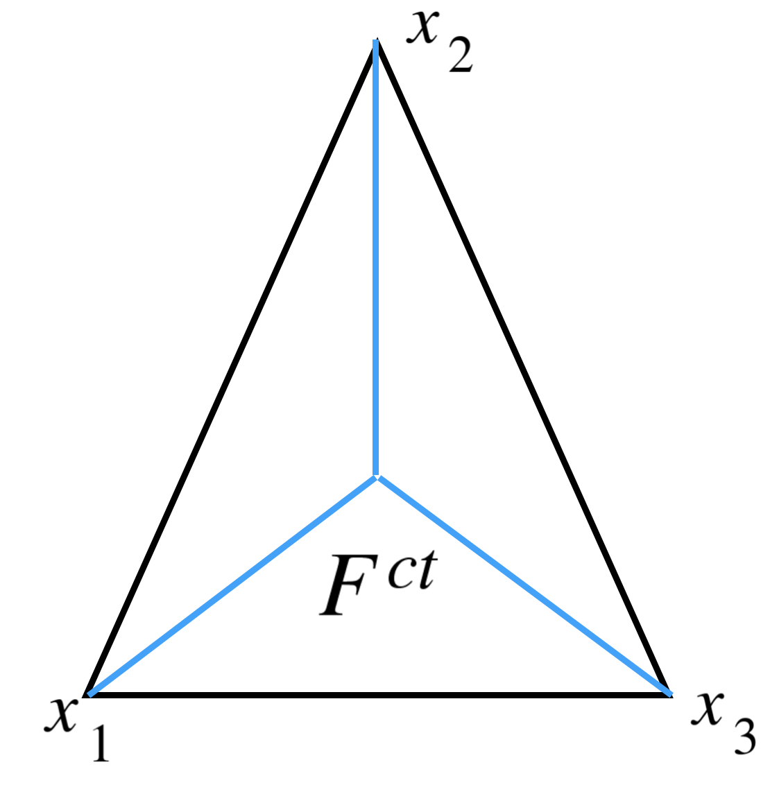
(a) A representation of $F^{ct}$ and $\Delta_{1}^{I}(F^{ct})$ (indicated in blue).

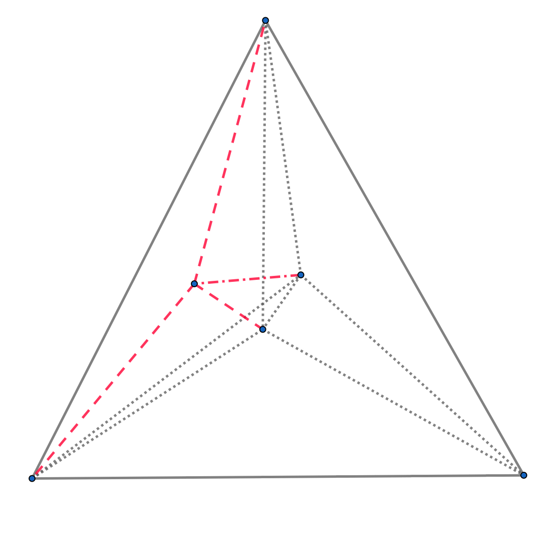
(b) Alfeld refinement and Worsey-Farin refinement (local) indicated in red

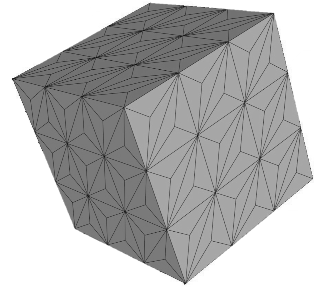
(c) Worsey-Farin refinement (global)

Figure 1. The Worsey-Farin Splits

2.3. Differential identities involving matrix and vector fields

We adopt the notation used in [13]. Let $F\in\Delta_{2}(T)$, and recall $n_{\scriptscriptstyle{F}}$ is the unit normal vector pointing out of $T$. Fix two tangent vectors $t_{1},t_{2}$ such that the ordered set $(b_{1},b_{2},b_{3})=(t_{1},t_{2},n_{\scriptscriptstyle{F}})$ is an orthonormal right-handed basis of $\mathbb{R}^{3}$. Any matrix field $u:T\to\mathbb{R}^{3\times 3}$ can be written as $\sum_{i,j=1}^{3}u_{ij}b_{i}b_{j}^{\prime}$ with scalar components $u_{ij}:T\to\mathbb{R}$. Let $u_{nn}=n_{\scriptscriptstyle{F}}^{\prime}un_{\scriptscriptstyle{F}}$ and ${\rm tr}_{\scriptscriptstyle{F}}u=\sum_{i=1}^{2}t_{i}^{\prime}ut_{i}.$ With $s\in\mathbb{R}^{3}$, let

(2.4) $$u_{{\scriptscriptstyle{F\!F}}}=\sum_{i,j=1}^{2}u_{ij}t_{i}t_{j}^{\prime},\qquad u_{Fs}=\sum_{i=1}^{2}(s^{\prime}ut_{i})t_{i}^{\prime},\qquad u_{sF}=\sum_{i=1}^{2}(t_{i}^{\prime}us)t_{i},.$$

Equivalently, $u_{{\scriptscriptstyle{F\!F}}}=QuQ$, $u_{Fs}=s^{\prime}uQ,$ and $u_{sF}=Qus$, where $P=n_{\scriptscriptstyle{F}}n_{\scriptscriptstyle{F}}^{\prime}$ and $Q=I-P$. Next, for scalar-valued (component) functions $\phi,w_{i},q_{i}$ and $u_{ij}$, we write the standard surface operators as

$${\rm grad}_{\scriptscriptstyle{F}}\phi=(\partial_{t_{1}}\phi)t_{1}+(\partial_{t_{2}}\phi)t_{2}, {\rm grad}_{\scriptscriptstyle{F}}(w_{1}t_{1}+w_{2}t_{2})=t_{1}({\rm grad}_{\scriptscriptstyle{F}}w_{1})^{\prime}+t_{2}({\rm grad}_{\scriptscriptstyle{F}}w_{2})^{\prime},$$

$${\rm rot}_{\scriptscriptstyle{F}}\phi=(\partial_{t_{2}}\phi)t_{1}-(\partial_{t_{1}}\phi)t_{2}, {\rm rot}_{\scriptscriptstyle{F}}(q_{1}t_{1}^{\prime}+q_{2}t_{2}^{\prime})=t_{1}({\rm rot}_{\scriptscriptstyle{F}}q_{1})^{\prime}+t_{2}({\rm rot}_{\scriptscriptstyle{F}}q_{2})^{\prime},$$

$$\operatorname{curl}_{\scriptscriptstyle{F}}(w_{1}t_{1}+w_{2}t_{2})=\partial_{t_{1}}w_{2}-\partial_{t_{2}}w_{1}, \operatorname{curl}_{\scriptscriptstyle{F}}u_{{\scriptscriptstyle{F\!F}}}=t_{1}^{\prime}\,\operatorname{curl}_{\scriptscriptstyle{F}}(u_{Ft_{1}})^{\prime}+t_{2}^{\prime}\,\operatorname{curl}_{\scriptscriptstyle{F}}(u_{Ft_{2}})^{\prime},$$

$${\rm div}_{\scriptscriptstyle{F}}(w_{1}t_{1}+w_{2}t_{2})=\partial_{t_{1}}w_{1}+\partial_{t_{2}}w_{2}, {\rm div}_{\scriptscriptstyle{F}}u_{{\scriptscriptstyle{F\!F}}}=t_{1}^{\prime}\,{\rm div}_{\scriptscriptstyle{F}}(u_{Ft_{1}})^{\prime}+t_{2}^{\prime}\,{\rm div}_{\scriptscriptstyle{F}}(u_{Ft_{2}})^{\prime}.$$

These operators are defined such that they are consistent with the conventions in [13]. In particular, we define ${\rm rot}_{\scriptscriptstyle{F}}$, such that the resulting operator ${\rm airy}_{\scriptscriptstyle{F}}$ mimics the three-dimensional operator, ${\rm inc}\,$. For a vector function $v$, denote $v_{\scriptscriptstyle{F}}=Qv=n_{\scriptscriptstyle{F}}\times(v\times n_{\scriptscriptstyle{F}})$. It is easy to see that

(2.5) $$n_{\scriptscriptstyle{F}}\cdot{\rm curl}\,v ={\rm curl}\,_{\scriptscriptstyle{F}}v_{\scriptscriptstyle{F}},\quad ({\rm grad}\,v)_{{\scriptscriptstyle{F\!F}}}={\rm grad}_{\scriptscriptstyle{F}}v_{\scriptscriptstyle{F}},$$

$$\quad n_{\scriptscriptstyle{F}}\times{\rm rot}_{\scriptscriptstyle{F}}\phi ={\rm grad}_{\scriptscriptstyle{F}}\phi,\quad {\rm div}\,v_{\scriptscriptstyle{F}}={\rm div}_{\scriptscriptstyle{F}}v_{\scriptscriptstyle{F}}.$$

Definition 2.2.

For a tangential vector function $v$ on the face $F\in\Delta_{2}(T)$, write $v=\sum\limits_{i=1}^{2}v_{i}t_{i}$ with $v_{i}=v\cdot t_{i}$. We define the orthogonal complement of $v$ as

$$v^{\perp}=v_{2}t_{1}-v_{1}t_{2}.$$

Using this definition and the standard surface operators introduced above, it is easy to see the following identities:

(2.6) $${\rm div}_{\scriptscriptstyle{F}}v^{\perp}=\operatorname{curl}_{\scriptscriptstyle{F}}v,\quad v^{\perp}\cdot t_{e}=v\cdot s_{e},\quad v^{\perp}=v\times n_{\scriptscriptstyle{F}}.$$

We also define the space of rigid body displacements within $\mathbb{R}^{3}$ and the face $F$:

(2.7) $$\mathsf{R} =\{a+b\times x:a,b\in\mathbb{R}^{3}\}$$

(2.8) $$\mathsf{R}(F) =\{at_{1}+bt_{2}+c((x\cdot t_{1})t_{2}-(x\cdot t_{2})t_{1}):a,b,c\in\mathbb{R}\}.$$

Definition 2.3.

Set $\mathbb{V}=\mathbb{R}^{3}$, and $\mathbb{M}_{k\times k}=\mathbb{R}^{k\times k}$.

1. The skew-symmetric operator ${\rm skw}:\mathbb{M}_{k\times k}\rightarrow\mathbb{M}_{k\times k}$ and the symmetric operator ${\rm sym}:\mathbb{M}_{k\times k}\rightarrow\mathbb{M}_{k\times k}$ are defined as follows: for any $M\in\mathbb{M}_{k\times k}$,

   $${\rm skw}(M)=\frac{1}{2}(M-M^{\prime});\quad{\rm sym}(M)=\frac{1}{2}(M+M^{\prime}).$$

   Denote the range of ${\rm skw}$ and ${\rm sym}$ as $\mathbb{K}_{k}={\rm skw}(\mathbb{M}_{k\times k})$ and $\mathbb{S}_{k}={\rm sym}(\mathbb{M}_{k\times k})$, respectively.

2. Define the operator $\Xi:\mathbb{M}_{3\times 3}\rightarrow\mathbb{M}_{3\times 3}$ by $\Xi M=M^{\prime}-{\rm tr}(M)\mathbb{I}$, where $\mathbb{I}$ is the $3\times 3$ identity matrix.

3. The three-dimensional symmetric gradient and incompatibility operators are given, respectively, by:

   $$\varepsilon={\rm sym}\,{\rm grad},\quad{\rm inc}\,=\operatorname{curl}(\operatorname{curl})^{\prime}.$$

4. The operators ${\rm mskw}\,:\mathbb{V}\rightarrow\mathbb{K}_{3}$ and ${\rm vskw}:\mathbb{M}_{3\times 3}\to\mathbb{V}$ are given by

   $${\rm mskw}\,\begin{pmatrix}v_{1}\\ v_{2}\\ v_{3}\end{pmatrix}=\begin{pmatrix}0&-v_{3}&v_{2}\\ v_{3}&0&-v_{1}\\ -v_{2}&v_{1}&0\end{pmatrix},\qquad{\rm vskw}:={\rm mskw}\,^{-1}\circ{\rm skw}.$$

5. The two-dimensional surface differential operators on a face $F$ are given by

   $$\varepsilon_{\scriptscriptstyle{F}}={\rm sym}\,{\rm grad}_{\scriptscriptstyle{F}},\quad{\rm airy}_{\scriptscriptstyle{F}}={\rm rot}_{\scriptscriptstyle{F}}({\rm rot}_{\scriptscriptstyle{F}})^{\prime},\quad{\rm inc}_{\scriptscriptstyle{F}}:=\operatorname{curl}_{F}(\operatorname{curl}_{F})^{\prime}.$$

6. The two-dimensional skew operator defined on either a scalar or matrix-valued function is defined, respectively, as

   $${\rm skew}\,u=\begin{bmatrix}0&u\\ -u&0\end{bmatrix};\quad{\rm skew}\,\begin{bmatrix}u_{11}&u_{12}\\ u_{21}&u_{22}\end{bmatrix}=u_{21}-u_{12}.$$

7. The transpose operator $\tau$ is defined as: $\tau\,u=u^{\prime}$.

It is simple to see that $\Xi$ is invertible with $\Xi^{-1}M=M^{\prime}-\frac{1}{2}{\rm tr}(M)\mathbb{I}$. Furthermore, the following identities hold:

(2.9a) $${\rm div}\,\Xi=2{\rm vskw}\,{\rm curl}\,,$$

(2.9b) $$\Xi{\rm grad}=-{\rm curl}\,\,{\rm mskw}\,,$$

(2.9c) $${\rm{\rm curl}\,\Xi^{-1}{\rm curl}\,}{\rm mskw}\,=-{\rm curl}\,\Xi^{-1}\Xi{\rm grad}=-{\rm curl}\,{\rm grad}=0,$$

(2.9d) $$2\,{\rm vskw}\,{\rm{\rm curl}\,\Xi^{-1}{\rm curl}\,}={\rm div}\,\Xi\Xi^{-1}{\rm curl}\,={\rm div}\,{\rm curl}\,=0,$$

(2.9e) $$\text{tr}({\rm curl}\,{\rm sym})=0,\quad{\rm{\rm curl}\,\Xi^{-1}{\rm curl}\,}{\rm sym}=\operatorname{curl}(\operatorname{curl}{\rm sym})^{\prime}={\rm inc}\,{\rm sym}.$$

On a two-dimensional face $F$, there also holds

(2.10a) $${\rm div}_{\scriptscriptstyle{F}}\,{\rm airy}_{\scriptscriptstyle{F}}={\rm div}_{\scriptscriptstyle{F}}\,{\rm rot}_{\scriptscriptstyle{F}}\,\tau\,({\rm rot}_{\scriptscriptstyle{F}})=0,$$

(2.10b) $${\rm inc}_{\scriptscriptstyle{F}}\,{\rm sym}={\rm inc}_{\scriptscriptstyle{F}},\quad{\rm inc}_{\scriptscriptstyle{F}}\,\varepsilon_{\scriptscriptstyle{F}}=\operatorname{curl}_{\scriptscriptstyle{F}}\,\tau\,\operatorname{curl}_{\scriptscriptstyle{F}}{\rm grad}_{\scriptscriptstyle{F}}=0,$$

(2.10c) $$\operatorname{curl}_{\scriptscriptstyle{F}}\,{\rm skew}=\tau\,{\rm grad}_{\scriptscriptstyle{F}}.$$

The following lemma states additional identities used throughout the paper. Its proof is found in [13, Lemma 5.7].

Lemma 2.4.

For a sufficiently smooth matrix-valued function $u$,

(2.11a) $$s^{\prime}\,({\rm curl}\,u)\,n_{\scriptscriptstyle{F}}\, =\operatorname{curl}_{\scriptscriptstyle{F}}(u_{{\scriptscriptstyle{F}}s})^{\prime},\text{ for any }s\in\mathbb{R}^{3},$$

(2.11b) $$\big{[}({\rm curl}\,u)^{\prime}\big{]}_{{{\scriptscriptstyle{F}}n}} =\operatorname{curl}_{\scriptscriptstyle{F}}u_{{\scriptscriptstyle{F\!F}}}.$$

If in addition $$u$$ is symmetric, then

(2.11c) $$({\rm inc}\,u)_{nn} ={\rm inc}_{\scriptscriptstyle{F}}\,u_{\scriptscriptstyle{F\!F}},$$

(2.11d) $$({\rm inc}\,u)_{{{\scriptscriptstyle{F}}n}} =\operatorname{curl}_{\scriptscriptstyle{F}}\big{[}({\rm curl}\,u)^{\prime}\big{]}_{{\scriptscriptstyle{F\!F}}},$$

(2.11e) $${\rm tr}_{\scriptscriptstyle{F}}{\rm curl}\,u =-\operatorname{curl}_{\scriptscriptstyle{F}}(u_{{{\scriptscriptstyle{F}}n}})^{\prime}.$$

For a sufficiently smooth vector-valued function $$v$$,

(2.11f) $$2({\rm curl}\,\varepsilon(v))^{\prime} ={\rm grad}\,{\rm curl}\,v,$$

(2.11g) $$2\left[({\rm curl}\,\varepsilon(v))^{\prime}\right]_{{\scriptscriptstyle{F\!F}}} ={\rm grad}_{\scriptscriptstyle{F}}({\rm curl}\,v)_{\scriptscriptstyle{F}},$$

(2.11h) $${\rm curl}\,v =n_{\scriptscriptstyle{F}}(\operatorname{curl}_{\scriptscriptstyle{F}}v_{\scriptscriptstyle{F}})+{\rm rot}_{\scriptscriptstyle{F}}(v\cdot n_{\scriptscriptstyle{F}})+n_{\scriptscriptstyle{F}}\times\partial_{n}v,$$

(2.11i) $$2[\varepsilon(v)]_{n{\scriptscriptstyle{F}}} =2[\varepsilon(v)_{{{\scriptscriptstyle{F}}n}}]^{\prime}={\rm grad}_{\scriptscriptstyle{F}}(v\cdot n_{\scriptscriptstyle{F}})+\partial_{n}v_{\scriptscriptstyle{F}},$$

(2.11j) $${\rm tr}_{\scriptscriptstyle{F}}({\rm rot}_{\scriptscriptstyle{F}}v_{\scriptscriptstyle{F}}^{\prime}) ={\rm curl}\,_{\scriptscriptstyle{F}}v_{\scriptscriptstyle{F}}.$$

2.4. Hilbert spaces

We summarize the definitions of Hilbert spaces which we use to define the discrete spaces. For any $T\in\mathcal{T}_{h}$, we commonly use $\mathring{(\cdot)}$ to denote the corresponding spaces with vanishing traces; see the following two examples:

$$\mathring{H}({\rm div},T):=\{v\in H({\rm div},T):v\cdot n|_{\partial T}=0\},\quad\mathring{H}({\rm curl}\,,T):=\{v\in H({\rm curl}\,,T):v\times n|_{\partial T}=0\}.$$

In addition, for any face $F\in\Delta_{2}(T)$ with $T\in\mathcal{T}_{h}$, we define the following spaces by using surface operators in Section 2.3:

$$H({\rm div}_{\scriptscriptstyle{F}},F):=\{v\in[L^{2}(F)]^{2}:{\rm div}_{\scriptscriptstyle{F}}v\in L^{2}(F)\},\mathring{H}({\rm div}_{\scriptscriptstyle{F}},F):=\{v\in H({\rm div}_{\scriptscriptstyle{F}},F):v\cdot s|_{\partial F}=0\},$$

$$H({\rm curl}_{\scriptscriptstyle{F}},F):=\{v\in[L^{2}(F)]^{2}:\operatorname{curl}_{F}v\in L^{2}(F)\},\mathring{H}({\rm curl}_{\scriptscriptstyle{F}},F):=\{v\in H({\rm curl}_{\scriptscriptstyle{F}},F):v\cdot t|_{\partial F}=0\},$$

$$H({\rm grad}_{\scriptscriptstyle{F}},F):=\{v\in L^{2}(F):{\rm grad}_{F}v\in L^{2}(F)\},\mathring{H}({\rm grad}_{\scriptscriptstyle{F}},F):=\{v\in H({\rm grad}_{\scriptscriptstyle{F}},F):v|_{\partial F}=0\},$$

where $s$ denotes the outward unit normal of $\partial F$ and $t$ denotes the unit tangential of $\partial F$.

3. Discrete complexes on Clough-Tocher splits

Recall a Worsey-Farin split of a tetrahedron induces a Clough-Tocher split on each of its faces. As a result, to construct degrees of freedom and commuting projections for discrete three-dimensional elasticity complexes on Worsey-Farin splits, we first derive two-dimensional discrete elasticity complexes on Clough-Tocher splits. Throughout this section, $F\in\Delta_{2}(\mathcal{T}_{h})$ is a face of the (unrefined) triangulation $\mathcal{T}_{h}$, and $F^{ct}$ denotes its Clough-Tocher refinement with respect to the split point $m_{F}$ (arising from the Worsey-Farin refinement of $\mathcal{T}_{h}$).

3.1. de Rham complexes

As an intermediate step to derive elasticity complexes on $F^{ct}$, we first state several discrete de Rham complexes with various levels of smoothness. First, we define the Nédélec spaces (without and with boundary conditions) on the Clough–Tocher split:

$$V_{{\rm div},r}^{1}(F^{\mathop{\mathrm{ct}\,}}):=\{v\in H({\rm div}_{\scriptscriptstyle{F}},F):v|_{Q}\in[\mathcal{P}_{r}({\color[rgb]{0,0,0}\tau})]^{2},\tau\in F^{\mathop{\mathrm{ct}\,}}\},\quad \mathring{V}^{1}_{{\rm div},r}(F^{\mathop{\mathrm{ct}\,}}):=V_{{\rm div},r}^{1}(F^{\mathop{\mathrm{ct}\,}})\cap\mathring{H}({\rm div}_{\scriptscriptstyle{F}},F)$$

$$V_{\operatorname{curl},r}^{1}(F^{\mathop{\mathrm{ct}\,}}):=\{v\in H(\operatorname{curl}_{\scriptscriptstyle{F}},F):v|_{\tau}\in{[\mathcal{P}_{r}({\color[rgb]{0,0,0}\tau})]^{2}},\tau\in F^{\mathop{\mathrm{ct}\,}}\},\quad \mathring{V}^{1}_{{\operatorname{curl}},r}(F^{\mathop{\mathrm{ct}\,}}):=V_{\rm curl,r}^{1}(F^{\mathop{\mathrm{ct}\,}})\cap\mathring{H}({\operatorname{curl}}_{\scriptscriptstyle{F}},F),$$

$${V}_{r}^{2}(F^{\mathop{\mathrm{ct}\,}}):=\{v\in L^{2}(F):v|_{\tau}\in\mathcal{P}_{r}({\color[rgb]{0,0,0}\tau}),\tau\in F^{\mathop{\mathrm{ct}\,}}\},\quad \mathring{V}_{r}^{2}(F^{\mathop{\mathrm{ct}\,}}):=V_{r}^{2}(F^{\mathop{\mathrm{ct}\,}})\cap L^{2}_{0}(F),$$

and the Lagrange spaces,

$$\mathsf{X}_{r}^{0}(F^{\mathop{\mathrm{ct}\,}}):=V_{r}^{2}(F^{\mathop{\mathrm{ct}\,}})\cap H({\rm grad}_{\scriptscriptstyle{F}},F),\quad \mathring{\mathsf{X}}_{r}^{0}(F^{\mathop{\mathrm{ct}\,}}):=\mathsf{X}_{r}^{0}(F^{\mathop{\mathrm{ct}\,}})\cap\mathring{H}({\rm grad}_{\scriptscriptstyle{F}},F),$$

$$\mathsf{X}_{r}^{1}(F^{\mathop{\mathrm{ct}\,}}):=[\mathsf{X}_{r}^{0}(F^{\mathop{\mathrm{ct}\,}})]^{2},\quad \mathring{\mathsf{X}}_{r}^{1}(F^{\mathop{\mathrm{ct}\,}}):=[\mathring{\mathsf{X}}_{r}^{0}(F^{\mathop{\mathrm{ct}\,}})]^{2},$$

$$\mathsf{X}_{r}^{2}(F^{\mathop{\mathrm{ct}\,}}):=\mathsf{X}_{r}^{0}(F^{\mathop{\mathrm{ct}\,}}),\quad \mathring{\mathsf{X}}_{r}^{2}(F^{\mathop{\mathrm{ct}\,}}):=\mathring{\mathsf{X}}_{r}^{0}(F^{\mathop{\mathrm{ct}\,}})\cap L^{2}_{0}(F).$$

Note that superscripts in the notation for the spaces refer to the order of the corresponding differential forms.

Finally, we define the (smooth) piecewise polynomial subspaces with $C^{1}$ continuity.

$$S_{r}^{0}(F^{\mathop{\mathrm{ct}\,}}):=\{v\in\mathsf{X}_{r}^{0}(F^{\mathop{\mathrm{ct}\,}}):\ {\rm grad}_{\scriptscriptstyle{F}}\,v\in{\mathsf{X}_{r-1}^{1}(F^{\mathop{\mathrm{ct}\,}})}\},$$

$$\mathring{S}_{r}^{0}(F^{\mathop{\mathrm{ct}\,}}):=\{v\in\mathring{\mathsf{X}}_{r}^{0}(F^{\mathop{\mathrm{ct}\,}}):\ {\rm grad}_{\scriptscriptstyle{F}}\,v\in{\mathring{\mathsf{X}}_{r-1}^{1}(F^{\mathop{\mathrm{ct}\,}})}\},$$

$$\mathcal{R}_{r}^{0}(F^{\mathop{\mathrm{ct}\,}}):=\{v\in S_{r}^{0}(F^{\mathop{\mathrm{ct}\,}}):v|_{\partial F}=0\}.$$

The first space $S^{0}_{r}(F^{\mathop{\mathrm{ct}\,}})$ is the so-called Hsieh-Clough-Tocher $C^{1}$ finite element space [16]. Several combinations of these spaces form exact sequences, as summarized in the following theorem.

Theorem 3.1.

Let $r\geq 3$. The following sequences are exact [6, 19].

(3.1a) $$\mathbb{R}\ {\xrightarrow{\hskip 14.22636pt}}\ {{\mathsf{X}}}_{r}^{0}(F^{\mathop{\mathrm{ct}\,}})\ \stackrel{{\scriptstyle{\rm grad}_{\scriptscriptstyle{F}}}}{{\xrightarrow{\hskip 14.22636pt}}}\ {{V}}_{\operatorname{curl},r-1}^{1}(F^{\mathop{\mathrm{ct}\,}})\ \stackrel{{\scriptstyle\operatorname{curl}_{\scriptscriptstyle{F}}}}{{\xrightarrow{\hskip 14.22636pt}}}\ {{V}}_{r-2}^{2}(F^{\mathop{\mathrm{ct}\,}})\ \xrightarrow{\hskip 14.22636pt}\ 0,$$

(3.1b) $$\mathbb{R}\ {\xrightarrow{\hskip 14.22636pt}}\ {S}_{r}^{0}(F^{\mathop{\mathrm{ct}\,}})\ \stackrel{{\scriptstyle{\rm grad}_{\scriptscriptstyle{F}}}}{{\xrightarrow{\hskip 14.22636pt}}}\ {\mathsf{X}}_{r-1}^{1}(F^{\mathop{\mathrm{ct}\,}})\ \stackrel{{\scriptstyle\operatorname{curl}_{\scriptscriptstyle{F}}}}{{\xrightarrow{\hskip 14.22636pt}}}\ {V}_{r-2}^{2}(F^{\mathop{\mathrm{ct}\,}})\ \xrightarrow{\hskip 14.22636pt}\ 0,$$

(3.1c) $$0\ {\xrightarrow{\hskip 14.22636pt}}\ {\mathring{\mathsf{X}}}_{r}^{0}(F^{\mathop{\mathrm{ct}\,}})\ \stackrel{{\scriptstyle{\rm grad}_{\scriptscriptstyle{F}}}}{{\xrightarrow{\hskip 14.22636pt}}}\ {\mathring{V}}_{\operatorname{curl},r-1}^{1}(F^{\mathop{\mathrm{ct}\,}})\ \stackrel{{\scriptstyle\operatorname{curl}_{\scriptscriptstyle{F}}}}{{\xrightarrow{\hskip 14.22636pt}}}\ {\mathring{V}}_{r-2}^{2}(F^{\mathop{\mathrm{ct}\,}})\ \xrightarrow{\hskip 14.22636pt}\ 0,$$

(3.1d) $$0\ {\xrightarrow{\hskip 14.22636pt}}\ \mathring{S}_{r}^{0}(F^{\mathop{\mathrm{ct}\,}})\ \stackrel{{\scriptstyle{\rm grad}_{\scriptscriptstyle{F}}}}{{\xrightarrow{\hskip 14.22636pt}}}\ \mathring{\mathsf{X}}_{r-1}^{1}(F^{\mathop{\mathrm{ct}\,}})\ \stackrel{{\scriptstyle\operatorname{curl}_{\scriptscriptstyle{F}}}}{{\xrightarrow{\hskip 14.22636pt}}}\ \mathring{V}_{r-2}^{2}(F^{\mathop{\mathrm{ct}\,}})\ \xrightarrow{\hskip 14.22636pt}\ 0.$$

Theorem 3.1 has an alternate form that follows from a rotation of the coordinate axes, where the operators ${\rm grad}_{F}$ and $\operatorname{curl}_{F}$ are replaced by ${\rm rot}_{F}$ and ${\rm div}_{F}$, respectively.

Corollary 3.2.

Let $r\geq 3$. The following sequences are exact [6, 19].

(3.2a) $$\mathbb{R}\ {\xrightarrow{\hskip 14.22636pt}}\ {{\mathsf{X}}}_{r}^{0}(F^{\mathop{\mathrm{ct}\,}})\ \stackrel{{\scriptstyle{\rm rot}_{\scriptscriptstyle{F}}}}{{\xrightarrow{\hskip 14.22636pt}}}\ {{V}}_{{\rm div},r-1}^{1}(F^{\mathop{\mathrm{ct}\,}})\ \stackrel{{\scriptstyle{\rm div}_{\scriptscriptstyle{F}}}}{{\xrightarrow{\hskip 14.22636pt}}}\ {{V}}_{r-2}^{2}(F^{\mathop{\mathrm{ct}\,}})\ \xrightarrow{\hskip 14.22636pt}\ 0,$$

(3.2b) $$\mathbb{R}\ {\xrightarrow{\hskip 14.22636pt}}\ {S}_{r}^{0}(F^{\mathop{\mathrm{ct}\,}})\ \stackrel{{\scriptstyle{\rm rot}_{\scriptscriptstyle{F}}}}{{\xrightarrow{\hskip 14.22636pt}}}\ {\mathsf{X}}_{r-1}^{1}(F^{\mathop{\mathrm{ct}\,}})\ \stackrel{{\scriptstyle{\rm div}_{\scriptscriptstyle{F}}}}{{\xrightarrow{\hskip 14.22636pt}}}\ {V}_{r-2}^{2}(F^{\mathop{\mathrm{ct}\,}})\ \xrightarrow{\hskip 14.22636pt}\ 0,$$

(3.2c) $$0\ {\xrightarrow{\hskip 14.22636pt}}\ {\mathring{\mathsf{X}}}_{r}^{0}(F^{\mathop{\mathrm{ct}\,}})\ \stackrel{{\scriptstyle{\rm rot}_{\scriptscriptstyle{F}}}}{{\xrightarrow{\hskip 14.22636pt}}}\ {\mathring{V}}_{{\rm div}\,,r-1}^{1}(F^{\mathop{\mathrm{ct}\,}})\ \stackrel{{\scriptstyle{\rm div}_{\scriptscriptstyle{F}}}}{{\xrightarrow{\hskip 14.22636pt}}}\ {\mathring{V}}_{r-2}^{2}(F^{\mathop{\mathrm{ct}\,}})\ \xrightarrow{\hskip 14.22636pt}\ 0,$$

(3.2d) $$0\ {\xrightarrow{\hskip 14.22636pt}}\ \mathring{S}_{r}^{0}(F^{\mathop{\mathrm{ct}\,}})\ \stackrel{{\scriptstyle{\rm rot}_{\scriptscriptstyle{F}}}}{{\xrightarrow{\hskip 14.22636pt}}}\ \mathring{\mathsf{X}}_{r-1}^{1}(F^{\mathop{\mathrm{ct}\,}})\ \stackrel{{\scriptstyle{\rm div}_{\scriptscriptstyle{F}}}}{{\xrightarrow{\hskip 14.22636pt}}}\ \mathring{V}_{r-2}^{2}(F^{\mathop{\mathrm{ct}\,}})\ \xrightarrow{\hskip 14.22636pt}\ 0.$$

3.2. Elasticity complexes

In order to construct elasticity sequences in three dimensions, we need some elasticity complexes on the two-dimensional Clough-Tocher splits. The main results of this section are very similar to the ones found [15] (with spaces slightly different) and can be proved with the techniques there. However, to be self-contained, we provide the proof of the main result, Theorem 3.4 in an appendix. Let $\mathbb{V}_{2}$ denote the plane $n^{\perp}$ where $n$ is a unit normal to $F^{\mathop{\mathrm{ct}\,}}$; clearly $\mathbb{V}_{2}$ is isomorphic to $\mathbb{R}^{2}$. Then the two-dimensional elasticity complexes utilize these:

(3.3a) $$\mathring{Q}_{{\rm inc},r}^{1}(F^{\mathop{\mathrm{ct}\,}}):=\{v\in\mathring{\mathsf{X}}_{r}^{1}(F^{\mathop{\mathrm{ct}\,}})\otimes\mathbb{V}_{2}:\ \operatorname{curl}_{\scriptscriptstyle{F}}v\in{\mathring{V}_{{\rm curl},r-1}^{1}(F^{\mathop{\mathrm{ct}\,}})}\},$$

(3.3b) $$\mathring{Q}_{{\rm inc},r}^{1,s}(F^{\mathop{\mathrm{ct}\,}}):=\{{\rm sym}(u):u\in\mathring{Q}_{{\rm inc},r}^{1}(F^{\mathop{\mathrm{ct}\,}})\},$$

(3.3c) $$Q^{1}_{r}(F^{\mathop{\mathrm{ct}\,}}):=\{u\in V_{{\rm div},r}^{1}(F^{\mathop{\mathrm{ct}\,}})\otimes\mathbb{V}_{2}:{\rm skew}(u)=0\},$$

(3.3d) $$\tilde{Q}^{1}_{r}(F^{\mathop{\mathrm{ct}\,}}):=\{u\in\mathsf{X}_{r}^{1}(F^{\mathop{\mathrm{ct}\,}})\otimes\mathbb{V}_{2}:{\rm skew}(u)=0\}\subset Q^{1}_{r}(F^{\mathop{\mathrm{ct}\,}}),$$

(3.3e) $$\mathring{Q}^{2}_{r}(F^{\mathop{\mathrm{ct}\,}}):=\{u\in V^{2}_{r}(F^{\mathop{\mathrm{ct}\,}}):u\perp\mathcal{P}_{1}(F)\}.$$

We further let $Q_{r}^{\perp}$ be the subspace of $Q_{r}^{1}(F^{\mathop{\mathrm{ct}\,}})$ that is $L^{2}(F)$-orthogonal to $\tilde{Q}^{1}_{r}(F^{\mathop{\mathrm{ct}\,}})$. We then have $Q_{r}^{1}(F^{\mathop{\mathrm{ct}\,}})=Q_{r}^{\perp}\oplus\tilde{Q}^{1}_{r}(F^{\mathop{\mathrm{ct}\,}})$, and

(3.4) $$\dim Q_{r}^{\perp}=\dim Q^{1}_{r}(F^{\mathop{\mathrm{ct}\,}})-\dim\tilde{Q}^{1}_{r}(F^{\mathop{\mathrm{ct}\,}}).$$

Lemma 3.3 (Lemma 5.8 in [13]).

Let $u$ be a sufficiently smooth matrix-valued function, and let $\phi$ be a smooth scalar-valued function. Then there holds the following integration-by-parts identity:

(3.5) $$\int_{F}({\rm inc}_{\scriptscriptstyle{F}}\,u)\,\phi=\int_{F}u\colon{\rm airy}_{\scriptscriptstyle{F}}(\phi)+\int_{\partial F}(\operatorname{curl}_{\scriptscriptstyle{F}}u)t\,\phi ds+\int_{\partial F}ut\cdot({\rm rot}_{\scriptscriptstyle{F}}\phi)^{\prime}.$$

Consequently, if $u\in\mathring{Q}_{{\rm inc},r-1}^{1}(F^{\mathop{\mathrm{ct}\,}})$ is symmetric and $\phi\in\mathcal{P}_{1}(F)$, then $\int_{F}({\rm inc}_{\scriptscriptstyle{F}}\,u)\,\phi=0$.

The next theorem is the main result of this section, where exact local discrete elasticity complexes are presented on Clough-Tocher splits. Its proof is given in Appendix A.

Theorem 3.4.

Let $r\geq 3$. The following elasticity sequences are exact.

(3.6) $$0\ {\xrightarrow{\hskip 14.22636pt}}\ \mathring{{S}}_{r+1}^{0}(F^{\mathop{\mathrm{ct}\,}})\otimes\mathbb{V}_{2}\ \stackrel{{\scriptstyle{\varepsilon}_{\scriptscriptstyle{F}}}}{{\xrightarrow{\hskip 14.22636pt}}}\ \mathring{Q}_{{\rm inc},r}^{1,s}(F^{\mathop{\mathrm{ct}\,}})\ \stackrel{{\scriptstyle{\rm inc}_{\scriptscriptstyle{F}}}}{{\xrightarrow{\hskip 14.22636pt}}}\ \mathring{Q}^{2}_{r-2}(F^{\mathop{\mathrm{ct}\,}})\ \xrightarrow{\hskip 14.22636pt}\ 0,$$

(3.7) $$\mathcal{P}_{1}(F)\ \stackrel{{\scriptstyle\subset}}{{\xrightarrow{\hskip 14.22636pt}}}\ {{S}}_{r}^{0}(F^{\mathop{\mathrm{ct}\,}})\ \stackrel{{\scriptstyle{\rm airy}_{\scriptscriptstyle{F}}}}{{\xrightarrow{\hskip 14.22636pt}}}\ Q^{1}_{r-2}(F^{\mathop{\mathrm{ct}\,}})\ \stackrel{{\scriptstyle{\rm div}_{\scriptscriptstyle{F}}}}{{\xrightarrow{\hskip 14.22636pt}}}\ V^{2}_{r-3}(F^{\mathop{\mathrm{ct}\,}})\otimes\mathbb{V}_{2}\ \xrightarrow{\hskip 14.22636pt}\ 0.$$

3.3. Dimension counts

We summarize the dimension counts of the discrete spaces on the Clough-Tocher split in Table 1 which will be used in the construction elasticity complex in three dimensions. These dimensions are mostly found in [21] and follow from Theorem 3.1 and the rank-nullity theorem. Likewise, the dimension of $Q^{1}_{r}(F^{ct})$ follows from Theorem 3.4.

Table 1. Dimension counts of the canonical (two–dimensional) Nédélec, Lagrange, and smooth spaces with respect to the Clough–Tocher split. Here, $\dim V_{{\rm div},r}^{1}(F^{\mathop{\mathrm{ct}\,}})=\dim V_{\operatorname{curl},r}^{1}(F^{\mathop{\mathrm{ct}\,}})=:\dim V_{r}^{1}(F^{\mathop{\mathrm{ct}\,}})$

	$k=0$	$k=1$	$k=2$
$\dim V_{r}^{k}(F^{\mathop{\mathrm{ct}\,}})$	—	$3(r+1)^{2}$	$\frac{3}{2}(r+1)(r+2)$
$\dim\mathring{V}_{r}^{k}(F^{\mathop{\mathrm{ct}\,}})$	—	$3r(r+1)$	$\frac{3}{2}(r+1)(r+2)-1$
$\dim\mathsf{X}_{r}^{k}(F^{\mathop{\mathrm{ct}\,}})$	$\frac{1}{2}(3r^{2}+3r+2)$	$3r^{2}+3r+2$	$\frac{1}{2}(3r^{2}+3r+2)$
$\dim\mathring{\mathsf{X}}_{r}^{k}(F^{\mathop{\mathrm{ct}\,}})$	$\frac{1}{2}(3r^{2}-3r+2)$	$3r^{2}-3r+2$	$\frac{3}{2}r(r-1)$
$\dim S_{r}^{k}(F^{\mathop{\mathrm{ct}\,}})$	$\frac{3}{2}(r^{2}-r+2)$	—	—
$\dim\mathcal{R}_{r}^{k}(F^{\mathop{\mathrm{ct}\,}})$	$\frac{3}{2}(r-1)(r-2)$ [25]	—	—
$\dim Q_{r}^{k}(F^{\mathop{\mathrm{ct}\,}})$	—	$\frac{3}{2}(3r^{2}+5r+2)$	—

4. Local discrete sequences on Worsey-Farin splits

4.1. de Rham complexes

Similar to the two-dimensional setting in Section 3, the starting point to construct discrete 3D elasticity complexes are the de Rham complexes consisting of piecewise polynomial spaces. The Nédélec spaces with respect to the local Worsey-Farin split $T^{wf}$ are given as

$$V_{r}^{1}(T^{wf}):=[\mathcal{P}_{r}(T^{wf})]^{3}\cap H(\operatorname{curl},T),\qquad \mathring{V}_{r}^{1}(T^{wf}):=V_{r}^{1}(T^{wf})\cap\mathring{H}(\operatorname{curl},T),$$

$$V_{r}^{2}(T^{wf}):=[\mathcal{P}_{r}(T^{wf})]^{3}\cap H({\rm div},T),\qquad \mathring{V}_{r}^{2}(T^{wf}):=V_{r}^{2}(T^{wf})\cap\mathring{H}({\rm div},T),$$

$$V_{r}^{3}(T^{wf}):=\mathcal{P}_{r}(T^{wf}), \mathring{V}_{r}^{3}(T^{wf}):=V_{r}^{3}(T^{wf})\cap L^{2}_{0}(T).$$

The Lagrange spaces on $T^{wf}$ are defined by

$$\mathsf{X}_{r}^{0}(T^{wf}):=\mathcal{P}_{r}(T^{wf})\cap H^{1}(T),\qquad \mathring{\mathsf{X}}_{r}^{0}(T^{wf}):=\mathsf{X}_{r}^{0}(T^{wf})\cap\mathring{H}^{1}(T),$$

$$\mathsf{X}_{r}^{1}(T^{wf}):=[\mathsf{X}_{r}^{0}(T^{wf})]^{3}, \mathring{\mathsf{X}}_{r}^{1}(T^{wf}):=[\mathring{\mathsf{X}}_{r}^{0}(T^{wf})]^{3},$$

$${\color[rgb]{0,0,0}\mathsf{X}_{r}^{2}(T^{wf}):=\mathsf{X}_{r}^{1}(T^{wf}),} {\color[rgb]{0,0,0}\mathring{\mathsf{X}}_{r}^{2}(T^{wf}):=\mathring{\mathsf{X}}_{r}^{1}(T^{wf}),}$$

and the discrete spaces with additional smoothness are

$$S_{r}^{0}(T^{wf}):=\{u\in\mathsf{X}_{r}^{0}(T^{wf}):{\rm grad}\,u\in\mathsf{X}_{r-1}^{1}(T^{wf})\},$$

$$\mathring{S}_{r}^{0}(T^{wf}):=\{u\in\mathring{\mathsf{X}}_{r}^{0}(T^{wf}):{\rm grad}\,u\in\mathring{\mathsf{X}}_{r-1}^{1}(T^{wf})\},$$

$$S_{r}^{1}(T^{wf}):=\{u\in\mathsf{X}_{r}^{1}(T^{wf}):{\rm curl}\,u\in\mathsf{X}_{r-1}^{1}(T^{wf})\},$$

$$\mathring{S}_{r}^{1}(T^{wf}):=\{u\in\mathring{\mathsf{X}}_{r}^{1}(T^{wf}):{\rm curl}\,u\in\mathring{\mathsf{X}}_{r-1}^{1}(T^{wf})\}.$$

We also define the intermediate spaces

$${\mathcal{V}}_{r}^{2}(T^{wf}):=\{v\in V_{r}^{2}(T^{wf}):{\color[rgb]{0,0,0}v\times n|_{F}}\text{ is continuous on each }F\in\Delta_{2}(T)\},$$

$$\mathring{\mathcal{V}}_{r}^{2}(T^{wf}):=\{v\in\mathcal{V}_{r}^{2}(T^{wf}):{\color[rgb]{0,0,0}v\cdot n|_{F}}=0\text{ on each }F\in\Delta_{2}(T)\},$$

$${\mathcal{V}}_{r}^{3}(T^{wf}):=\{q\in V_{r}^{3}(T^{wf}):{\color[rgb]{0,0,0}q|_{F}}\text{ is continuous on each }F\in\Delta_{2}(T)\},$$

$$\mathring{\mathcal{V}}_{r}^{3}:=\mathcal{V}_{r}^{3}(T^{wf})\cap L_{0}^{2}(T).$$

and note that

$$S_{r}^{0}(T^{wf})\subset\mathsf{X}^{0}_{r}(T^{wf}),\qquad {\color[rgb]{0,0,0}S_{r}^{1}(T^{wf})}\subset\mathsf{X}^{1}_{r}(T^{wf})\subset V_{r}^{1}(T^{wf}),$$

$$\mathsf{X}^{2}_{r}(T^{wf})\subset\mathcal{V}_{r}^{2}(T^{wf})\subset V_{r}^{2}(T^{wf}),\quad \mathcal{V}_{r}^{3}(T^{wf})\subset V_{r}^{3}(T^{wf}),$$

with similar inclusions holding for the analogous spaces with boundary conditions.

The next lemma summarizes the exactness properties of several (local) complexes using these spaces. Its proof is found in [21, Theorem 3.1-3.2].

Lemma 4.1.

The following sequences are exact for any $r\geq 3$.

(4.1a) $$\mathbb{R}\xrightarrow{\subset}\mathsf{X}_{r}^{0}(T^{wf})\xrightarrow{{\rm grad}}V_{r-1}^{1}(T^{wf})\xrightarrow{{\rm curl}\,}V_{r-2}^{2}(T^{wf})\xrightarrow{{\rm div}\,}V_{r-3}^{3}(T^{wf})\rightarrow 0,$$

(4.1b) $$0\rightarrow\mathring{\mathsf{X}}_{r}^{0}(T^{wf})\xrightarrow{{\rm grad}}\mathring{V}_{r-1}^{1}(T^{wf})\xrightarrow{{\rm curl}\,}\mathring{V}_{r-2}^{2}(T^{wf})\xrightarrow{{\rm div}\,}\mathring{V}_{r-3}^{3}(T^{wf})\rightarrow 0,$$

(4.1c) $$\mathbb{R}\xrightarrow{\subset}S_{r}^{0}(T^{wf})\xrightarrow{{\rm grad}}\mathsf{X}_{r-1}^{1}(T^{wf})\xrightarrow{{\rm curl}\,}V_{r-2}^{2}(T^{wf})\xrightarrow{{\rm div}\,}V_{r-3}^{3}(T^{wf})\rightarrow 0,$$

(4.1d) $$0\rightarrow\mathring{S}_{r}^{0}(T^{wf})\xrightarrow{{\rm grad}}\mathring{\mathsf{X}}_{r-1}^{1}(T^{wf})\xrightarrow{{\rm curl}\,}\mathring{\mathcal{V}}_{r-2}^{2}(T^{wf})\xrightarrow{{\rm div}\,}\mathring{V}_{r-3}^{3}(T^{wf})\rightarrow 0.$$

(4.1e) $$\mathbb{R}\xrightarrow{\subset}S_{r}^{0}(T^{wf})\xrightarrow{{\rm grad}}S_{r-1}^{1}(T^{wf})\xrightarrow{{\rm curl}\,}\mathsf{X}_{r-2}^{2}(T^{wf})\xrightarrow{{\rm div}\,}V_{r-3}^{3}(T^{wf})\rightarrow 0.$$

(4.1f) $$0\rightarrow\mathring{S}_{r}^{0}(T^{wf})\xrightarrow{{\rm grad}}\mathring{S}_{r-1}^{1}(T^{wf})\xrightarrow{{\rm curl}\,}\mathring{\mathsf{X}}_{r-2}^{2}(T^{wf})\xrightarrow{{\rm div}\,}\mathring{\mathcal{V}}_{r-3}^{3}(T^{wf})\rightarrow 0.$$

4.2. Dimension counts

The dimensions of the spaces in Section 4.1 are summarized in Table 2. These counts essentially from Lemma 4.1 and the rank-nullity theorem; see [21] for details.

Table 2. Dimension counts of the canonical Nédélec, Lagrange spaces and smoother spaces on a WF split. Here $a^{+}=\max(a,0)$.

	$k=0$	$k=1$	$k=2$	$k=3$
$V_{r}^{k}(T^{wf})$	$(2r+1)(r^{2}+r+1)$	$2(r+1)(3r^{2}+6r+4)$	$3(r+1)(r+2)(2r+3)$	$2(r+1)(r+2)(r+3)$
$\mathring{V}_{r}^{k}(T^{wf})$	$(2r-1)(r^{2}-r+1)$	$2(r+1)(3r^{2}+1)$	$3(r+1)(r+2)(2r+1)$	$2r^{3}+12r^{2}+22r+11$
$\mathsf{X}_{r}^{k}(T^{wf})$	$(2r+1)(r^{2}+r+1)$	$3(2r+1)(r^{2}+r+1)$	$3(2r+1)(r^{2}+r+1)$	$(2r+1)(r^{2}+r+1)$
$\mathring{\mathsf{X}}_{r}^{k}(T^{wf})$	$(2r-1)(r^{2}-r+1)$	$3(2r-1)(r^{2}-r+1)$	$3(2r-1)(r^{2}-r+1)$	$(r-1)(2r^{2}-r+2)$
$\mathring{\mathcal{V}}_{r}^{k}(T^{wf})$	—	—	$6r^{3}+21r^{2}+9r+2$	$2r^{3}+12r^{2}+10r+3$
$S_{r}^{k}(T^{wf})$	$2r^{3}-6r^{2}+10r-2$	$3r(2r^{2}-3r+5)$	$6r^{3}+8r+2$	$(2r+1)(r^{2}+r+1)$
$\mathring{S}_{r}^{0}(T^{wf})$	$\big{(}2(r-2)(r-3)(r-4)\big{)}^{+}$	$\big{(}3(2r-3)(r-2)(r-3)\big{)}^{+}$	$\big{(}2(r-2)(3r^{2}-6r+4)\big{)}^{+}$	$(r-1)(2r^{2}-r+2)$

4.3. Elasticity complex for stresses with weakly imposed symmetry

In this section we will apply Proposition 2.1 to the de-Rham sequences on Worsey-Farin splits. This gives rise to a derived complex useful for analyzing mixed methods for elasticity with weakly imposed stress symmetry. From this intermediate step, an elasticity sequence with strong symmetry will readily follow. We start with the following definition and lemma.

Definition 4.2.

Let $\mu\in\mathring{\mathsf{X}}_{1}^{0}(T^{wf})$ be the unique continuous, piecewise linear polynomial that vanishes on $\partial T$ and takes the value $1$ at the incenter of $T$.

Lemma 4.3.

1. The map $\Xi:\mathsf{X}_{r}^{1}(T^{wf})\otimes\mathbb{V}\rightarrow\mathsf{X}_{r}^{2}(T^{wf})\otimes\mathbb{V}$ is a bijection.

2. The following inclusions hold ${\rm vskw}\,(V_{r-2}^{2}(T^{wf})\otimes\mathbb{V})\subset V_{r-2}^{3}(T^{wf})\otimes\mathbb{V}$ and
   ${\rm vskw}\,(\mathring{\mathcal{V}}_{r-2}^{2}(T^{wf})\otimes\mathbb{V})\subset\mathcal{V}_{r-2}^{3}(T^{wf})\otimes\mathbb{V}$, for any $r\geq 3$.

3. The mappings ${\rm vskw}:V^{2}_{r-2}(T^{wf})\otimes\mathbb{V}\rightarrow V^{3}_{r-2}(T^{wf})\otimes\mathbb{V}$ and ${\rm vskw}:\mathring{\mathcal{V}}^{2}_{r-2}(T^{wf})\otimes\mathbb{V}\rightarrow\mathcal{V}^{3}_{r-2}(T^{wf})\otimes\mathbb{V}$ are both surjective, for any $r\geq 3$.

Proof.

Both (1) and (2) are trivial to verify and hence we only prove (3). For any $r\geq 3$, let $v\in V^{3}_{r-2}(T^{wf})\otimes\mathbb{V}$. By the exactness of (4.1e), there exists a function $z\in\mathsf{X}_{r-2}^{2}(T^{wf})\otimes\mathbb{V}$ such that ${\rm div}\,z=v$. Since $\Xi$ is a bijection from $\mathsf{X}_{r-2}^{1}(T^{wf})\otimes\mathbb{V}$ to $\mathsf{X}_{r-2}^{2}(T^{wf})\otimes\mathbb{V}$, we have $q=\Xi^{-1}z\in\mathsf{X}_{r-2}^{1}(T^{wf})\otimes\mathbb{V}$. Thus, by setting $w={\rm curl}\,q\in V_{r-2}^{2}(T^{wf})\otimes\mathbb{V}$ we obtain

$$2{\rm vskw}(w)=2{\rm vskw}\,{\rm curl}\,(q)=2{\rm vskw}\,{\rm curl}\,(\Xi^{-1}z)={\rm div}\,\Xi(\Xi^{-1}z)=v,$$

where we used (2.9a). We conclude ${\rm vskw}:V^{2}_{r-2}(T^{wf})\otimes\mathbb{V}\rightarrow V^{3}_{r-2}(T^{wf})\otimes\mathbb{V}$ is a surjection.

We now prove the analogous result with boundary condition. Let $v\in\mathcal{V}^{3}_{r-2}(T^{wf})\otimes\mathbb{V}$, and let $M\in\mathbb{M}_{3\times 3}$ be a constant matrix such that $\int_{T}2{\rm vskw}\,M=\frac{1}{\int_{T}\mu}{\int_{T}v}$. Then, by taking $\tilde{w}=\mu M$, we have $\tilde{w}\in\mathring{\mathcal{V}}_{1}^{2}(T^{wf})\otimes\mathbb{V}$ with $\int_{T}2{\rm vskw}\,\tilde{w}=\int_{T}v$. Therefore, we have $v-2\,{\rm vskw}(\tilde{w})\in\mathring{\mathcal{V}}^{3}_{r-2}(T^{wf})\otimes\mathbb{V}$ and the exactness of (4.1f) yields the existence of $z\in\mathring{\mathsf{X}}_{r-1}^{2}(T^{wf})\otimes\mathbb{V}$, such that ${\rm div}\,z=v-2{\rm vskw}(\tilde{w})$. Let $q=\Xi^{-1}z\in\mathring{\mathsf{X}}_{r-1}^{1}(T^{wf})\otimes\mathbb{V}$, and from (4.1d), we have $w:={\rm curl}\,(q)+\tilde{w}\in\mathring{\mathcal{V}}_{r-2}^{2}(T^{wf})\otimes\mathbb{V}$. Finally, using (2.9a)

$$2{\rm vskw}(w)=2{\rm vskw}\,{\rm curl}\,(\Xi^{-1}z)+2{\rm vskw}(\tilde{w})={\rm div}\,z+2{\rm vskw}(\tilde{w})=v.$$

This shows the surjectivity of ${\rm vskw}:\mathring{\mathcal{V}}^{2}_{r-2}(T^{wf})\otimes\mathbb{V}\rightarrow\mathcal{V}^{3}_{r-2}(T^{wf})\otimes\mathbb{V}$, thus completing the proof. ∎

Using the complexes (4.1c)-(4.1f) and the two identities (2.9a)-(2.9b), we construct the following commuting diagrams:

(4.2)

(4.3)

Note that the top sequence of (4.3) is slightly different from (4.1f), as the mean-value constraint is not imposed on $\mathcal{V}_{r-2}(T^{wf})\otimes\mathbb{V}$. This is due to the surjective property of the mapping ${\rm vskw}:(\mathring{\mathcal{V}}_{r-2}^{2}(T^{wf})\otimes\mathbb{V})\to\mathcal{V}_{r-2}^{3}(T^{wf})\otimes\mathbb{V}$ established in Lemma 4.3.

Theorem 4.4.

The following sequences are exact for any $r\geq 3$:

(4.4) $$\begin{bmatrix}S_{r+1}^{0}(T^{wf})\!\otimes\!\mathbb{V}\\ S_{r}^{0}(T^{wf}\!\otimes\!\mathbb{V})\end{bmatrix}\xrightarrow{[{\rm grad},-{\rm mskw}\,]}S_{r}^{1}(T^{wf})\!\otimes\!\mathbb{V}\xrightarrow{{\rm{\rm curl}\,\Xi^{-1}{\rm curl}\,}}{V}_{r-2}^{2}(T^{wf})\!\otimes\!\mathbb{V}\xrightarrow{\left[\begin{smallmatrix}2{\rm vskw}\\ {\rm div}\,\end{smallmatrix}\right]}\begin{bmatrix}V^{3}_{r-2}(T^{wf})\!\otimes\!\mathbb{V}\\ {V}_{r-3}^{3}(T^{wf})\!\otimes\!\mathbb{V}\end{bmatrix}.$$

(4.5) $$\begin{bmatrix}\mathring{S}_{r+1}^{0}(T^{wf})\otimes\mathbb{V}\\ \mathring{S}_{r}^{0}(T^{wf}\otimes\mathbb{V})\end{bmatrix}\xrightarrow{[{\rm grad},-{\rm mskw}\,]}\mathring{S}_{r}^{1}(T^{wf})\otimes\mathbb{V}\xrightarrow{{\rm{\rm curl}\,\Xi^{-1}{\rm curl}\,}}\mathring{\mathcal{V}}_{r-2}^{2}(T^{wf})\otimes\mathbb{V}\xrightarrow{\left[\begin{smallmatrix}2{\rm vskw}\\ {\rm div}\,\end{smallmatrix}\right]}\begin{bmatrix}\mathcal{V}^{3}_{r-2}(T^{wf})\otimes\mathbb{V}\\ \mathring{V}_{r-3}^{3}(T^{wf})\otimes\mathbb{V}\end{bmatrix}.$$

Moreover, the last operator in (4.4) is surjective.

Proof.

Lemma 4.3 tells us that $\Xi:\mathsf{X}_{r-1}^{1}(T^{wf})\otimes\mathbb{V}\rightarrow\mathsf{X}_{r-1}^{2}(T^{wf})\otimes\mathbb{V}$ is a bijection. With the exactness of (4.1c)-(4.1f) for $r\geq 3$ and Proposition 2.1, we see that these two sequences are exact. The surjectivity of the last map is guaranteed by Proposition 2.1 and Lemma 4.3. ∎

4.4. Elasticity sequence

Now we are ready to describe the local discrete elasticity sequence on Worsey-Farin splits. The discrete elasticity complexes with strong symmetry are formed by the following spaces:

$$U_{r+1}^{0}(T^{wf})=S_{r+1}^{0}(T^{wf})\otimes\mathbb{V}, \mathring{U}_{r+1}^{0}(T^{wf})=\mathring{S}_{r+1}^{0}(T^{wf})\otimes\mathbb{V},$$

$$U_{r}^{1}(T^{wf})=\{{\rm sym}(u):u\in S_{r}^{1}(T^{wf})\otimes\mathbb{V}\}, \mathring{U}_{r}^{1}(T^{wf})=\{{\rm sym}(u):u\in\mathring{S}_{r}^{1}(T^{wf})\otimes\mathbb{V}\},$$

$$U_{r-2}^{2}(T^{wf})=\{u\in V_{r-2}^{2}(T^{wf})\otimes\mathbb{V}:{\rm skw}\,u=0\}, \mathring{U}_{r-2}^{2}(T^{wf})=\{u\in\mathring{\mathcal{V}}_{r-2}^{2}(T^{wf})\otimes\mathbb{V}:{\rm skw}\,u=0\},$$

$$U_{r-3}^{3}(T^{wf})=V_{r-3}^{3}(T^{wf})\otimes\mathbb{V}, \mathring{U}_{r-3}^{3}(T^{wf})=\{u\in V_{r-3}^{3}(T^{wf})\otimes\mathbb{V}:u\perp\mathsf{R}\},$$

where we recall $\mathsf{R}$, defined in (2.7), is the space of rigid body displacements.

Theorem 4.5.

The following two sequences are discrete elasticity complexes and are exact for $r\geq 3$:

(4.6) $$\mathsf{R}\rightarrow{U}_{r+1}^{0}(T^{wf})\xrightarrow{\varepsilon}{U}_{r}^{1}(T^{wf})\xrightarrow{{\rm inc}\,}{U}_{r-2}^{2}(T^{wf})\xrightarrow{{\rm div}\,}{U}_{r-3}^{3}(T^{wf})\rightarrow 0,$$

and

(4.7) $$0\rightarrow\mathring{U}_{r+1}^{0}(T^{wf})\xrightarrow{\varepsilon}\mathring{U}_{r}^{1}(T^{wf})\xrightarrow{{\rm inc}\,}\mathring{U}_{r-2}^{2}(T^{wf})\xrightarrow{{\rm div}\,}\mathring{U}_{r-3}^{3}(T^{wf})\rightarrow 0.$$

Proof.

We first show that (4.6) is a complex. In order to do this, it suffices to show the operators map the space they are acting on into the subsequent space. To this end, let $u\in U_{r+1}^{0}(T^{wf})$, then by (4.1e) we have ${\rm grad}\,(u)\in S_{r}^{1}(T^{wf})\otimes\mathbb{V}$. Hence, $\varepsilon(u)={\rm sym}\,{\rm grad}\,(u)\in U_{r}^{1}(T^{wf})$. Now let $u\in U_{r}^{1}(T^{wf})$ which implies that $u={\rm sym}(w)$ with $w\in S_{r}^{1}(T^{wf})\otimes\mathbb{V}$. Thus by (2.9c) we have ${\rm{\rm curl}\,\Xi^{-1}{\rm curl}\,}u={\rm{\rm curl}\,\Xi^{-1}{\rm curl}\,}w\in V_{r-2}^{2}(T^{wf})\otimes\mathbb{V}$ and ${\rm skw}(u)=0$ due to (2.9d). Therefore, there holds ${\rm{\rm curl}\,\Xi^{-1}{\rm curl}\,}(u)\in{U}_{r-2}^{2}(T^{wf})$. Finally, for any $u\in{U}_{r-2}^{2}(T^{wf})\subset V_{r-2}^{2}(T^{wf})\otimes\mathbb{V}$, ${\rm div}\,u\in V_{r-3}^{3}(T^{wf})\otimes\mathbb{V}$.

Next, we prove exactness of the complex (4.6). Let $w\in{U}_{r-3}^{3}(T^{wf})$ and consider $(0,w)\in[V_{r-2}^{3}(T^{wf})\otimes\mathbb{V}]\times[V_{r-3}^{3}(T^{wf})\otimes\mathbb{V}]$. Due to the exactness of (4.4) in Theorem 4.4, there exists $v\in V_{r-2}^{2}(T^{wf})\otimes\mathbb{V}$ such that ${\rm div}\,v=w$ and $2{\rm vskw}(v)=0$. Thus, $v\in{U}_{r-2}^{2}(T^{wf})$.

Now let $w\in{U}_{r-2}^{2}(T^{wf})$ with ${\rm div}\,w=0$. Then by the exactness of (4.4), we have the existence of $v\in S_{r}^{1}(T^{wf})\otimes\mathbb{V}$ such that ${\rm{\rm curl}\,\Xi^{-1}{\rm curl}\,}v=w$. Setting $u={\rm sym}(v)\in{U}_{r}^{1}(T^{wf})$ yields ${\rm inc}\,u=w$ by (2.9c).

Finally, let $w\in{U}_{r}^{1}(T^{wf})$ with ${\rm inc}\,w=0$. Then $w={\rm sym}(v)$ for some $v\in S_{r}^{1}(T^{wf})\otimes\mathbb{V}$ and with (2.9c), ${\rm{\rm curl}\,\Xi^{-1}{\rm curl}\,}v={\rm{\rm curl}\,\Xi^{-1}{\rm curl}\,}w=0$. Due to the exactness of (4.4), we could find $(u,z)\in[S_{r+1}^{0}(T^{wf})\otimes\mathbb{V}]\times[S_{r}^{0}(T^{wf})\otimes\mathbb{V}]$ such that $v={\rm grad}\,u-{\rm mskw}\,(z)$. Therefore, $\varepsilon(u)={\rm sym}(v)=w$.

We can prove that (4.7) is a complex and it is exact very similar to above. The main difference is the surjectivity of the last map which we prove now. Let $w\in\mathring{U}_{r-3}^{3}(T^{wf})\subset\mathring{V}_{r-3}^{3}\otimes\mathbb{V}$. Then by the exactness of (4.1d), there exists $v\in\mathring{\mathcal{V}}_{r-2}^{2}(T^{wf})\otimes\mathbb{V}$ such that ${\rm div}\,v=w$. For any $c\in\mathbb{R}^{3}$ we have ${\rm grad}\,(c\times x)={\rm mskw}\,\,c$ and hence, using integration by parts

$$\int_{T}2{\rm vskw}\,v\cdot c=\int_{T}v\colon{\rm mskw}\,\,c=\int_{T}v\colon{\rm grad}\,(c\times x)=-\int_{T}{\rm div}\,v\cdot(c\times x)=-\int_{T}w\cdot(c\times x)=0,$$

where the last equality uses the fact $w\perp\mathsf{R}$. Therefore, ${\rm vskw}\,v\in\mathring{\mathcal{V}}_{r-2}^{3}(T^{wf})\otimes\mathbb{V}$ and by the exactness of (4.1f), we have an $m\in\mathring{\mathsf{X}}_{r-1}^{2}(T^{wf})\otimes\mathbb{V}$ such that ${\rm div}\,m=2{\rm vskw}\,v$. Let $u=v-{\rm curl}\,(\Xi^{-1}m)\in\mathring{\mathcal{V}}_{r-2}^{2}(T^{wf})\otimes\mathbb{V}$ and we see that $2{\rm vskw}\,u=2{\rm vskw}\,v-2{\rm vskw}\,{\rm curl}\,(\Xi^{-1}m)=0$ by (2.9a). Hence, $u\in\mathring{U}_{r-2}^{2}(T^{wf})$ and ${\rm div}\,u=w$. ∎

When $r\geq 4$, there holds $\mathsf{R}\subset{U}_{r-3}^{3}(T^{wf})$, so it is clear that

(4.8) $${U}_{r-3}^{3}(T^{wf})=\mathsf{R}\oplus\mathring{U}_{r-3}^{3}(T^{wf})\qquad\text{ for }r\geq 4.$$

On the other hand, when $r=3$, we need the following lemma for the calculation of dimensions of $\mathring{U}_{r-3}^{3}(T^{wf})$. Let $P_{\scriptscriptstyle{U}}$ be the $L^{2}$-orthogonal projection onto $U_{0}^{3}(T^{wf})$ and let $P_{\scriptscriptstyle{U}}\mathsf{R}:=\{P_{\scriptscriptstyle{U}}u:\ u\in\mathsf{R}\}$. The proof of the following lemma is provided in the appendix.

Lemma 4.6.

It holds,

(4.9) $${U}_{0}^{3}(T^{wf})=P_{\scriptscriptstyle{U}}\mathsf{R}\oplus\mathring{U}_{0}^{3}(T^{wf}),$$

and $\dim P_{\scriptscriptstyle{U}}\mathsf{R}=\dim\mathsf{R}=6$.

Using the exactness of the complexes (4.6)–(4.7) along with Table 2, we calculate the dimensions of the spaces in the next lemma.

Lemma 4.7.

When $r\geq 3$, we have:

(4.10) $$\dim{U}_{r+1}^{0}(T^{wf})=6r^{3}+12r+12, \dim\mathring{U}_{r+1}^{0}(T^{wf})=6r^{3}-36r^{2}+66r-36,$$

(4.11) $$\dim{U}_{r}^{1}(T^{wf})=12r^{3}-9r^{2}+15r+6, \dim\mathring{U}_{r}^{1}(T^{wf})=12r^{3}-63r^{2}+87r-18,$$

(4.12) $$\dim{U}_{r-2}^{2}(T^{wf})=12r^{3}-27r^{2}+15r, \dim\mathring{U}_{r-2}^{2}(T^{wf})=12r^{3}-45r^{2}+33r+12,$$

(4.13) $$\dim{U}_{r-3}^{3}(T^{wf})=6r^{3}-18r^{2}+12r, \dim\mathring{U}_{r-3}^{3}(T^{wf})=6r^{3}-18r^{2}+12r-6.$$

Proof.

By Lemma 4.3 and the rank-nullity theorem, we have

$$\dim{U}_{r-2}^{2}(T^{wf}) =\dim\ker(V_{r-2}^{2}(T^{wf})\otimes\mathbb{V},{\rm vskw})=\dim V_{r-2}^{2}(T^{wf})\otimes\mathbb{V}-\dim V_{r-2}^{3}(T^{wf})\otimes\mathbb{V}$$

$$=(6r^{3}-9r^{2}+3r)\times 3-2r(r+1)(r-1)\times 3=12r^{3}-27r^{2}+15r,$$

$$\dim\mathring{U}_{r-2}^{2}(T^{wf}) =\dim\ker(\mathring{\mathcal{V}}_{r-2}^{2}(T^{wf})\otimes\mathbb{V},{\rm vskw})=\dim\mathring{\mathcal{V}}_{r-2}^{2}(T^{wf})\otimes\mathbb{V}-\dim\mathcal{V}_{r-2}^{3}(T^{wf})\otimes\mathbb{V}$$

$$=(6(r-2)^{3}+21(r-2)^{2}+9(r-2)+2)\times 3$$

$$\leavevmode\nobreak\ \leavevmode\nobreak\ \leavevmode\nobreak\ \leavevmode\nobreak\ -2((r-2)^{3}+6(r-2)^{2}+5(r-2)+2)\times 3$$

$$=18r^{3}-45r^{2}-9r+60-(6r^{3}-42r+48)=12r^{3}-45r^{2}+33r+12.$$

The dimensions of ${U}_{r+1}^{0}(T^{wf})$, $\mathring{U}_{r+1}^{0}(T^{wf})$ and ${U}_{r-3}^{3}(T^{wf})$ are computed similarly using the dimensions of $S_{r+1}^{0}(T^{wf})$, $\mathring{S}_{r+1}^{0}(T^{wf})$ and $V_{r-3}^{3}(T^{wf})$. Also, using Lemma 4.6 when $r=3$ or (4.8) when $r\geq 4$, we obtain

$$\dim\mathring{U}_{r-3}^{3}(T^{wf})=\dim{U}_{r-3}^{3}(T^{wf})-6.$$

Using the exactness of the sequences (4.6) and (4.7) in Theorem 4.5, with the rank-nullity theorem, we have

$$\dim{U}_{r}^{1}(T^{wf}) =\dim{U}_{r+1}^{0}(T^{wf})+\dim{U}_{r-2}^{2}(T^{wf})-\dim{U}_{r-3}^{3}(T^{wf})-\dim\mathsf{R}$$

$$=12r^{3}-9r^{2}+15r+6,$$

$$\dim\mathring{U}_{r}^{1}(T^{wf}) =\dim\mathring{U}_{r+1}^{0}(T^{wf})+\dim\mathring{U}_{r-2}^{2}(T^{wf})-\dim\mathring{U}_{r-3}^{3}(T^{wf})$$

$$=12r^{3}-63r^{2}+87r-18.$$

∎

4.5. An equivalent characterization of $U^{1}_{r}(T^{wf})$ and $\mathring{U}_{r}^{1}(T^{wf})$

We will now show that $U_{r}^{1}(T^{wf})$ admits a characterization as a conforming subspace of the Sobolev space $H^{1}(\text{inc})$ appearing in (1.3). The next result will also help us find the local degrees of freedom of $U_{r}^{1}(T^{wf})$ and $\mathring{U}_{r}^{1}(T^{wf})$.

Theorem 4.8.

We have the following equivalent definitions of ${U}_{r}^{1}(T^{wf})$ and $\mathring{U}_{r}^{1}(T^{wf})$:

(4.14) $${U}_{r}^{1}(T^{wf})=\{u\in H^{1}(T;\mathbb{S}):u\in\mathcal{P}_{r}(T^{wf};\mathbb{S}),({\rm curl}\,u)^{\prime}\in V_{r-1}^{1}(T^{wf})\otimes\mathbb{V}\},$$

(4.15) $$\mathring{U}_{r}^{1}(T^{wf})=\{u\in\mathring{H}^{1}(T;\mathbb{S}):u\in\mathcal{P}_{r}(T^{wf};\mathbb{S}),({\rm curl}\,u)^{\prime}\in\mathring{V}_{r-1}^{1}(T^{wf})\otimes\mathbb{V},$$

$$\hskip 227.62204pt{\rm inc}(u)\in\mathring{\mathcal{V}}_{r-2}^{2}(T^{wf})\otimes\mathbb{V}\}.$$

Proof.

Let the right-hand side of (4.14) and (4.15) be denoted by $M_{r}$ and $\mathring{M}_{r}$, respectively. If $u\in{U}_{r}^{1}(T^{wf})$, then $u={\rm sym}(z)$ for some $z\in S_{r}^{1}(T^{wf})\otimes\mathbb{V}$, so (2.9e), (2.9b) and Definition 2.3 give

(4.16) $$({\rm curl}\,u)^{\prime}=\Xi^{-1}{\rm curl}\,u=\Xi^{-1}{\rm curl}\,z+{\rm grad}\,{\rm vskw}(z),$$

from which we conclude $({\rm curl}\,u)^{\prime}\in V_{r-1}^{1}(T^{wf})\otimes\mathbb{V}$. This proves the inclusion

(4.17) $${U}_{r}^{1}(T^{wf})\subset M_{r}.$$

Similarly, if $u\in\mathring{U}_{r}^{1}(T^{wf})$, then (4.16) for $z\in\mathring{S}_{r}^{1}(T^{wf})\otimes\mathbb{V}$, hence we have $({\rm curl}\,u)^{\prime}\in\mathring{V}_{r-1}^{1}(T^{wf})\otimes\mathbb{V}$. Moreover, using (2.9c) and the exact sequence (4.1d), we obtain

$${\rm inc}(u)={\rm{\rm curl}\,\Xi^{-1}{\rm curl}\,}(u)={\rm{\rm curl}\,\Xi^{-1}{\rm curl}\,}(z)\in{\rm curl}\,(\mathring{\mathsf{X}}_{r-1}^{1}(T^{wf})\otimes\mathbb{V})\subset\mathring{\mathcal{V}}_{r-2}^{2}(T^{wf})\otimes\mathbb{V}.$$

This proves

(4.18) $$\mathring{U}_{r}^{1}(T^{wf})\subset\mathring{M}_{r}.$$

We continue to prove the reverse inclusion of (4.14). For any $m\in M_{r}$, let $\sigma={\rm curl}\,({\rm curl}\,m)^{\prime}$ which immediately implies that ${\rm div}\,\sigma=0$. Moreover, by (2.9e) $\sigma={\rm{\rm curl}\,\Xi^{-1}{\rm curl}\,}(m)$ and by (2.9d) ${\rm vskw}(\sigma)=0$. Hence, we have $\sigma\in V_{r-2}^{2}(T^{wf})\otimes\mathbb{V}$, and by the exact sequence (4.4) there exists $w\in S_{r}^{1}(T^{wf})\otimes\mathbb{V}$ such that ${\rm{\rm curl}\,\Xi^{-1}{\rm curl}\,}(w)=\sigma$. Therefore, $w-m\in V_{r}^{1}(T^{wf})\otimes\mathbb{V}$ with ${\rm{\rm curl}\,\Xi^{-1}{\rm curl}\,}(w-m)=0$ and hence, by the exact sequence (4.1a), there exists $v\in{\mathsf{X}}_{r}^{0}(T^{wf})\otimes\mathbb{V}$ such that ${\rm grad}\,v=\Xi^{-1}{\rm curl}\,(w-m)$. Setting $z=m+{\rm vskw}(v)$ gives ${\rm sym}(z)=m$ and by (2.9b),

$${\rm curl}\,z={\rm curl}\,m+{\rm curl}\,{\rm mskw}\,v={\rm curl}\,m-\Xi{\rm grad}\,v={\rm curl}\,w\in{\color[rgb]{0,0,0}{\mathsf{X}}_{r-1}^{1}(T^{wf})\otimes\mathbb{V}}.$$

We conclude

(4.19) $$M_{r}\subset{U}_{r}^{1}(T^{wf}).$$

The reverse inclusion to prove (4.15) follows similar arguments, using the exact sequence (4.5) and (4.1b) in place of (4.4) and (4.1a), respectively. ∎

5. Local degrees of freedom for the elasticity complex on Worsey-Farin splits

In this section we present degrees of freedom for the discrete spaces arising in the elasticity complex. We first need to introduce some notation as follows. Recall that $T^{a}$ is the set of four tetrahedra obtained by connecting the vertices of $T$ with its incenter. For each $K\in T^{a}$, we denote the local Worsey-Farin splits of $K$ as $K^{wf}$, i.e.,

$$K^{wf}=\{S\in T^{wf}:\bar{S}\subset\bar{K}\}.$$

Then, similar to the discrete functions spaces on $T^{wf}$ defined in Section 4.1, we define spaces on $K^{wf}$ by taking their restriction:

$$\mathsf{X}_{r}^{0}(K^{wf}):=\{u|_{K}:u\in\mathsf{X}_{r}^{0}(T^{wf})\};\qquad S_{r}^{0}(K^{wf}):=\{u|_{K}:u\in S_{r}^{0}(T^{wf})\}.$$

Lemma 5.1.

Let $T\in\mathcal{T}_{h}$, and let $F\in\Delta_{2}(T)$. If $p\in\mathsf{X}_{r}^{0}(T^{wf})$ with $p=0$ on $F$, then ${\rm grad}\,p$ is continuous on $F$. In particular, the normal derivative $\partial_{n}p$ is continuous on $F$. In addition, if $p\in S_{r}^{0}(T^{wf})$ with $p=0$ on $F$, then ${\rm grad}\,p|_{\scriptscriptstyle{F}}\in S_{r-1}^{0}(F^{ct})\otimes\mathbb{V}$ and in particular, $\partial_{n}p|_{F}\in S_{r-1}^{0}(F^{\mathop{\mathrm{ct}\,}})$.

Proof.

Let $K\in T^{a}$ such that $F\in\Delta_{2}(K)$. Then, since $p$ vanishes on $F$, we have that $p=\mu q$ on $K$ where $q\in\mathsf{X}_{r-1}^{0}(K^{wf})$ and $\mu$ is the piecewise linear polynomial in Definition 4.2. We write ${\rm grad}\,p=\mu{\rm grad}\,q+q{\rm grad}\,\mu$, and since $\mu$ vanishes on $F$ and ${\rm grad}\,\mu$ is constant on $F$, we have ${\rm grad}\,p$ is continuous on $F$.

Furthermore, if $p\in S_{r}^{0}(T^{wf})$, then $p=\mu q$ on $K$ where $q\in S_{r-1}^{0}(K^{wf})$ because $\mu$ is a strictly positive polynomial on $K$. Hence by the same reasoning as the previous case, ${\rm grad}\,p|_{\scriptscriptstyle{F}}\in S_{r-1}^{0}(F^{ct})\otimes\mathbb{V}$. ∎

5.1. Dofs of $U^{0}$ space

Lemma 5.2.

A function $u\in{U}_{r+1}^{0}(T^{wf})$, with $r\geq 3$, is fully determined by the following dofs :

(5.1a) $$u(a), \qquad a\in\Delta_{0}(T), \qquad{\tiny{\text{${12}\leavevmode\nobreak\ {\rm{dofs}}$}}},$$

(5.1b) $${\rm grad}\,u(a), \qquad a\in\Delta_{0}(T), \qquad{\tiny{\text{${36}\leavevmode\nobreak\ {\rm{dofs}}$}}},$$

(5.1c) $$\int_{e}u\cdot\kappa, \qquad\kappa\in[\mathcal{P}_{r-3}(e)]^{3},\leavevmode\nobreak\ e\in\Delta_{1}(T), \qquad{\tiny{\text{${18(r-2)}\leavevmode\nobreak\ {\rm{dofs}}$}}},$$

(5.1d) $$\int_{e}\frac{\partial u}{\partial n_{e}^{\pm}}\cdot\kappa, \qquad\kappa\in[\mathcal{P}_{r-2}(e)]^{3},\leavevmode\nobreak\ e\in\Delta_{1}(T), \qquad{\tiny{\text{${36(r-1)}\leavevmode\nobreak\ {\rm{dofs}}$}}},$$

(5.1e) $$\int_{\scriptscriptstyle{F}}\varepsilon_{\scriptscriptstyle{F}}(u_{F})\colon\varepsilon_{\scriptscriptstyle{F}}(\kappa), \qquad\kappa\in[\mathring{S}_{r+1}^{0}(F^{ct})]^{2},F\in\Delta_{2}(T) \qquad{\tiny{\text{${12r^{2}-36r+24}\leavevmode\nobreak\ {\rm{dofs}}$}}},$$

(5.1f) $$\int_{\scriptscriptstyle{F}}[\varepsilon(u)]_{{{\scriptscriptstyle{F}}n}}\cdot\kappa, \qquad\kappa\in{\rm grad}_{\scriptscriptstyle{F}}\mathring{S}_{r+1}^{0}(F^{ct}),F\in\Delta_{2}(T) \qquad{\tiny{\text{${6r^{2}-18r+12}\leavevmode\nobreak\ {\rm{dofs}}$}}},$$

(5.1g) $$\int_{\scriptscriptstyle{F}}\partial_{n}(u\cdot n_{\scriptscriptstyle{F}})\kappa, \qquad\kappa\in{\mathcal{R}}_{r}^{0}(F^{ct}),F\in\Delta_{2}(T) \qquad{\tiny{\text{${6r^{2}-18r+12}\leavevmode\nobreak\ {\rm{dofs}}$}}},$$

(5.1h) $$\int_{\scriptscriptstyle{F}}\partial_{n}u_{F}\cdot\kappa, \qquad\kappa\in[{\mathcal{R}}_{r}^{0}(F^{ct})]^{2},F\in\Delta_{2}(T) \qquad{\tiny{\text{${12r^{2}-36r+24}\leavevmode\nobreak\ {\rm{dofs}}$}}},$$

(5.1i) $$\int_{T}\varepsilon(u)\colon\varepsilon(\kappa), \qquad\kappa\in\mathring{U}_{r+1}^{0}(T^{wf}), \qquad{\tiny{\text{${6(r-1)(r-2)(r-3)}\leavevmode\nobreak\ {\rm{dofs}}$}}},$$

where $\frac{\partial}{\partial n_{e}^{\pm}}$ represents two normal derivatives to edge $e$ and $\{n_{e}^{+},n_{e}^{-},t_{e}\}$ forms an edge-based orthonormal basis of $\mathbb{R}^{3}$.

Proof.

The dimension of ${U}_{r+1}^{0}(T^{wf})$ is $6r^{3}+12r+12$, which is equal to the sum of the given dofs .

Let $u\in{U}_{r+1}^{0}(T^{wf})$ such that it vanishes on the dofs   (5.1). On each edge $e\in\Delta_{1}(T)$, $u|_{e}=0$ by (5.1a)-(5.1c). Furthermore, ${\rm grad}\,u|_{e}=0$ by (5.1b) and (5.1d). Hence on any face $F\in\Delta_{2}(T)$, we have $u_{\scriptscriptstyle{F}}\in[\mathring{S}_{r+1}^{0}(F^{ct})]^{2}$. Then with dofs   (5.1e), $u_{\scriptscriptstyle{F}}=0$ on $F$. Now with Lemma 5.1 applied to $u_{\scriptscriptstyle{F}}\in S_{r+1}^{0}(T^{wf})\otimes\mathbb{V}_{2}$, we have $\partial_{n}u_{\scriptscriptstyle{F}}\in S_{r}^{0}(F^{ct})\otimes\mathbb{V}_{2}$. In addition, since ${\rm grad}\,u_{\scriptscriptstyle{F}}|_{\partial F}=0$, it follows that $\partial_{n}u_{\scriptscriptstyle{F}}\in[{\mathcal{R}}_{r}^{0}(F^{ct})]^{2}$ and with (5.1h), we have $\partial_{n}u_{\scriptscriptstyle{F}}=0$.

Using the identity (2.11i), we have $2[\varepsilon(u)]_{{{\scriptscriptstyle{F}}n}}=\partial_{n}u_{\scriptscriptstyle{F}}+{\rm grad}_{\scriptscriptstyle{F}}(u\cdot n_{\scriptscriptstyle{F}})={\rm grad}_{\scriptscriptstyle{F}}(u\cdot n_{\scriptscriptstyle{F}})$. With $u\cdot n_{\scriptscriptstyle{F}}\in S_{r+1}^{0}(F^{ct})$, we have in (5.1f), $[\varepsilon(u)]_{{{\scriptscriptstyle{F}}n}}=0$ and thus $u\cdot n_{\scriptscriptstyle{F}}=0$ on $F$. Now similar to $u_{\scriptscriptstyle{F}}$, with Lemma 5.1 applied to $u\cdot n_{\scriptscriptstyle{F}}$, we have $\partial_{n}(u\cdot n_{\scriptscriptstyle{F}})\in{\mathcal{R}}_{r}^{0}(F^{ct})$ and with (5.1g), we have $\partial_{n}(u\cdot n_{\scriptscriptstyle{F}})=0$.

Since $u|_{\partial T}=0$, all the tangential derivatives of $u$ vanish. With $\partial_{n}(u\cdot n_{\scriptscriptstyle{F}})=0$ and $\partial_{n}u_{\scriptscriptstyle{F}}=0$, we conclude that ${\rm grad}\,u|_{\partial T}=0$. Thus $u\in\mathring{U}_{r+1}^{0}(T^{wf})$, and (5.1i) shows that $u$ vanishes. ∎

5.2. Dofs of $U^{1}$ space

Before giving the dofs   of the space $U^{1}$ we need preliminary results to see the continuity of the functions involved. In the following lemmas, we use the jump operator $[\![{\cdot}]\!]$ and the set of internal edges of a split face $\Delta_{1}^{I}(F^{ct})$ given in Section 2.2. The proofs of the next four results are found in the appendix.

Lemma 5.3.

Let $\sigma\in V_{r}^{2}(T^{wf})\otimes\mathbb{V}$ with ${\rm skw}(\sigma)=0$. If $n_{\scriptscriptstyle{F}}^{\prime}\sigma\ell=0$ on $\partial T$ for some $\ell\in\mathbb{R}^{3}$, then $\sigma_{{\scriptscriptstyle{F}}\ell}\in V_{{\rm div},r}^{1}(F^{ct})$ on each $F\in\Delta_{2}(T)$.

Lemma 5.4.

Let $w\in V^{1}_{r-1}(T^{wf})\otimes\mathbb{V}$ such that $w^{\prime}\in V^{2}_{r-1}(T^{wf})\otimes\mathbb{V}$. If $w_{{{\scriptscriptstyle{F}}n}}=0$ on some $F\in\Delta_{2}(T)$, then we have

(5.2) $${\color[rgb]{0,0,0}[\![{t_{s}^{\prime}wn_{f}}]\!]_{e}=0};\quad[\![{s_{e}^{\prime}ws_{e}}]\!]_{e}=0,\qquad\text{ for all }e\in\Delta_{1}^{I}(F^{ct}).$$

On the other hand, if $w_{\scriptscriptstyle{F\!F}}=0$ on $F$, then we have

(5.3) $$[\![{t_{e}^{\prime}wn_{f}}]\!]_{e}=0;\quad[\![{t_{e}^{\prime}wn_{F}}]\!]_{e}=0,\qquad\text{ for all }e\in\Delta_{1}^{I}(F^{ct}).$$

Lemma 5.5.

Let $T$ be a tetrahedron, and let $\ell,m$ be two tangent vectors to a face $F\in\Delta_{2}(T)$ such that $\ell\cdot m=0$ and $\ell\times m=n_{\scriptscriptstyle{F}}$. Let $u\in\mathsf{X}_{r}^{1}(T^{wf})\otimes\mathbb{V}$ for some $r\geq 0$. If $u_{\scriptscriptstyle{F\!F}}=0$ on some $F\in\Delta_{2}(T)$, then

(5.4) $$[\![{\ell^{\prime}({\rm curl}\,u)m}]\!]_{e} =-[\![{{\rm grad}_{\scriptscriptstyle{F}}(u_{{{\scriptscriptstyle{F}}n}}\cdot\ell)\cdot\ell}]\!]_{e}, \qquad\text{ for all }e\in\Delta_{1}^{I}(F^{ct}),$$

(5.5) $$[\![{\ell^{\prime}({\rm curl}\,u)\ell}]\!]_{e} =-[\![{{\rm grad}_{\scriptscriptstyle{F}}(u_{{{\scriptscriptstyle{F}}n}}\cdot\ell)\cdot m}]\!]_{e}, \qquad\text{ for all }e\in\Delta_{1}^{I}(F^{ct}).$$

On the other hand, if $u_{n{\scriptscriptstyle{F}}}=0$ on $F$, then

(5.6) $$[\![{n_{F}^{\prime}({\rm curl}\,u)\ell}]\!]_{e}=[\![{({\rm grad}_{\scriptscriptstyle{F}}u_{nn})\cdot m}]\!]_{e},\qquad\text{ for all }e\in\Delta_{1}^{I}(F^{ct}).$$

Lemma 5.6.

Suppose $u\in{U}_{r}^{1}(T^{wf})$ and $w=(\operatorname{curl}u)^{\prime}$ are such that $u_{{\scriptscriptstyle{F\!F}}}$ and $w_{{{\scriptscriptstyle{F}}n}}$ vanish on a face $F\in\Delta_{2}(T)$. Then $w_{{\scriptscriptstyle{F\!F}}}-{\rm grad}_{\scriptscriptstyle{F}}{\color[rgb]{0,0,0}u_{n{\scriptscriptstyle{F}}}^{\perp}}$ is continuous on $F$. Furthermore, if $u=\varepsilon(v)$ for some $v\in{U}_{r+1}^{0}(T^{wf})$, then the following identity holds:

(5.7) $$w_{{\scriptscriptstyle{F\!F}}}=[(\operatorname{curl}\varepsilon(v))^{\prime}]_{{\scriptscriptstyle{F\!F}}}={\rm grad}_{\scriptscriptstyle{F}}{\color[rgb]{0,0,0}u_{n{\scriptscriptstyle{F}}}^{\perp}}+{\rm grad}_{\scriptscriptstyle{F}}(\partial_{n}v_{\scriptscriptstyle{F}}\times n_{\scriptscriptstyle{F}}).$$

In addition to (3.5) in Lemma 3.3, we need another identity to proceed with our construction. The following result is shown in [13, Lemma 5.8].

Lemma 5.7.

Let $u$ be a symmetric matrix-valued function with $[({\rm curl}\,u)^{\prime}]_{{\scriptscriptstyle{F\!F}}}t|_{\partial F}=0$ , $u|_{\partial F}=0$. Let $q\in\mathsf{R}(F)$ be defined in (2.8). Then there holds

(5.8) $$\int_{F}({\rm inc}\,u)_{{{\scriptscriptstyle{F}}n}}\cdot q=0.$$

Lemma 5.8.

A function $u\in{U}_{r}^{1}(T^{wf})$, with $r\geq 3$, is fully determined by the following vertex degrees of freedom

(5.9a) $$u(a), \quad a\in\Delta_{0}(T), {24}\leavevmode\nobreak\ {\rm{dofs}}$$

the following edge dofs   on all $$e\in\Delta_{1}(T),$$

(5.9b) $$\int_{e}u\colon\kappa, \quad\kappa\in{\rm sym}[\mathcal{P}_{r-2}(e)]^{3\times 3}, {36(r-1)}\leavevmode\nobreak\ {\rm{dofs}}$$

(5.9c) $$\int_{e}({\rm curl}\,u)^{\prime}t_{e}\cdot\kappa, \quad\kappa\in[\mathcal{P}_{r-1}(e)]^{3}, {18r}\leavevmode\nobreak\ {\rm{dofs}}$$

the following face dofs   on all $$F\in\Delta_{2}(T)$$,

(5.9d) $$\int_{F}({\rm inc\leavevmode\nobreak\ }u)_{{\scriptscriptstyle{F\!F}}}\colon\kappa, \quad\kappa\in Q_{r-2}^{\perp}, {12(r-2)}\leavevmode\nobreak\ {\rm{dofs}}$$

(5.9e) $$\int_{\scriptscriptstyle{F}}({\rm inc\leavevmode\nobreak\ }u)_{nn}\kappa, \quad\kappa\in\mathring{Q}^{2}_{r-2}(F^{\mathop{\mathrm{ct}\,}}), {6r^{2}-6r-12}\leavevmode\nobreak\ {\rm{dofs}}$$

(5.9f) $$\int_{\scriptscriptstyle{F}}({\rm inc\leavevmode\nobreak\ }u)_{{{\scriptscriptstyle{F}}n}}\cdot\kappa, \quad\kappa\in V_{{\rm div},r-2}^{1}(F^{ct})/\mathsf{R}(F), {12r^{2}-24r}\leavevmode\nobreak\ {\rm{dofs}}$$

(5.9g) $$\int_{F}u_{{\scriptscriptstyle{F\!F}}}\colon\kappa, \quad\kappa\in\varepsilon_{\scriptscriptstyle{F}}([\mathring{S}_{r+1}^{0}(F^{ct})]^{2}), {12(r^{2}-3r+2)}\leavevmode\nobreak\ {\rm{dofs}}$$

(5.9h) $$\int_{\scriptscriptstyle{F}}([({\rm curl}\,u)^{\prime}]_{{\scriptscriptstyle{F\!F}}}-{\rm grad}_{\scriptscriptstyle{F}}({\color[rgb]{0,0,0}u_{n{\scriptscriptstyle{F}}}^{\perp}}))\colon\kappa, \quad\kappa\in{\rm grad}_{\scriptscriptstyle{F}}[(\mathcal{R}_{r}^{0}(F^{ct})]^{2}, {12(r^{2}-3r+2)}\leavevmode\nobreak\ {\rm{dofs}}$$

(5.9i) $$\int_{F}u_{{{\scriptscriptstyle{F}}n}}\cdot\kappa, \quad\kappa\in{\rm grad}_{\scriptscriptstyle{F}}([\mathring{S}_{r+1}(F^{ct})]), {6(r^{2}-3r+2)}\leavevmode\nobreak\ {\rm{dofs}}$$

(5.9j) $$\int_{F}u_{nn}\kappa, \quad\kappa\in\mathcal{R}_{r}^{0}(F^{ct}), {6(r^{2}-3r+2)}\leavevmode\nobreak\ {\rm{dofs}}$$

and the following interior dofs ,

(5.9k) $$\int_{T}{\rm\leavevmode\nobreak\ inc}(u)\colon{\rm\leavevmode\nobreak\ inc}(\kappa), \quad\kappa\in\mathring{U}_{r}^{1}(T^{wf}), {6r^{3}-27r^{2}+21r+18}\leavevmode\nobreak\ {\rm{dofs}}$$

(5.9l) $$\int_{T}{\color[rgb]{0,0,0}u}\colon\varepsilon(\kappa), \quad\kappa\in\mathring{U}_{r+1}^{0}(T^{wf}), \quad{\tiny{\text{${6(r-1)(r-2)(r-3)}\leavevmode\nobreak\ {\rm{dofs}}$}}}.$$

Proof.

The dimension of ${U}_{r}^{1}(T^{wf})$ is $12r^{3}-9r^{2}+15r+6$, which is equal to the sum of the given dofs . Suppose that all dofs   (5.9) vanish for a $u\in U_{r}^{1}(T^{wf})$.

Step 0: Using the dofs   (5.9a, 5.9b) and (5.9c), we conclude

(5.10) $$u|_{e}=0,\quad({\rm curl}\,u)^{\prime}t|_{e}=0,\qquad{\rm for\leavevmode\nobreak\ }e\in\Delta_{1}(T).$$

Step 1: We show ${\rm inc}\,u\in\mathring{\mathcal{V}}_{r-2}^{2}(T^{wf})\otimes\mathbb{V}$.
By (2.11b) and (5.10), we have

$$0=n_{\scriptscriptstyle{F}}^{\prime}({\rm curl}\,u)^{\prime}t=(\operatorname{curl}_{\scriptscriptstyle{F}}u_{{\scriptscriptstyle{F\!F}}})t\quad\text{on $\partial F$ for each $F\in\Delta_{2}(T)$.}$$

Since $u$ is symmetric and continuous, by (2.11c), we see that $({\rm inc}\,u)_{nn}={\rm inc}_{\scriptscriptstyle{F}}\,u_{\scriptscriptstyle{F\!F}}$ with $u_{\scriptscriptstyle{F\!F}}\in\mathring{Q}_{{\rm inc},r}^{1,s}(F^{\mathop{\mathrm{ct}\,}})\subset\mathring{Q}_{{\rm inc},r}^{1}(F^{\mathop{\mathrm{ct}\,}})$. Thus, the complex (3.6) in Theorem 3.4 and the dofs   (5.9e) yield

(5.11) $$({\rm inc}\,u)_{nn}=0\qquad\text{on each $F\in\Delta_{2}(T)$.}$$

Next, Lemma 5.3 (with $\ell=n_{\scriptscriptstyle{F}}$ and $\sigma={\rm inc}\,u$) shows $({\rm inc}\,u)_{Fn}\in V^{1}_{{\rm div},r-2}(F^{ct})$. Therefore using the dofs   (5.9f) and (5.8) in Lemma 5.7, we conclude $({\rm inc}\,u)_{{{\scriptscriptstyle{F}}n}}=0$.

The identities $({\rm inc}\,u)_{nn}=0$ and $({\rm inc}\,u)_{{{\scriptscriptstyle{F}}n}}=0$ yield $({\rm inc}\,u)n_{\scriptscriptstyle{F}}=0$. So, by Lemma 5.3 (with $\ell=t_{1},t_{2}$), we see that $({\rm inc}\,u)_{\scriptscriptstyle{F\!F}}\in V_{{\rm div},r-2}^{1}(F^{ct})\otimes\mathbb{V}_{2}$. In particular, since $({\rm inc}\,u)_{\scriptscriptstyle{F\!F}}$ is symmetric, there holds $({\rm inc}\,u)_{\scriptscriptstyle{F\!F}}\in Q_{r-2}^{1}(F^{ct})$ (cf. (3.3c)). Thus by the dofs   (5.9d) and the definition of $Q^{\perp}_{r-2}(F^{ct})$ in Section 3, we have $({\rm inc}\,u)_{{\scriptscriptstyle{F\!F}}}\in L_{r}^{1}(F^{\mathop{\mathrm{ct}\,}})\otimes\mathbb{V}_{2}$. Therefore, we conclude ${\rm inc}\,u\in\mathring{\mathcal{V}}_{r-2}^{2}(T^{wf})\otimes\mathbb{V}$.

Step 2: We show $({\rm curl}\,u)^{\prime}\in\mathring{V}_{r-1}^{1}(T^{wf})\otimes\mathbb{V}$.
Using (5.11) and (2.11c), we have $0=({\rm inc}\,u)_{nn}={\rm inc}_{\scriptscriptstyle{F}}u_{{\scriptscriptstyle{F\!F}}}$. Thus by the exact sequence (3.6) in Theorem 3.4, there holds $u_{{\scriptscriptstyle{F\!F}}}=\varepsilon_{\scriptscriptstyle{F}}(\kappa)$ for some $\kappa\in\mathring{S}_{r+1}^{0}(F^{ct})\otimes\mathbb{V}_{2}$. We then conclude from the dofs   (5.9g) that $u_{{\scriptscriptstyle{F\!F}}}=0$ on each $F\in\Delta_{2}(F)$. Furthermore by (2.11b), $[({\rm curl}\,u)^{\prime}]_{Fn}={\rm curl}_{F}u_{{\scriptscriptstyle{F\!F}}}=0$.

Since $({\rm curl}\,u)^{\prime}\in V_{r-1}^{1}(T^{wf})\otimes\mathbb{V}$ by Theorem 4.8 and from (5.10)

$$[({\rm curl}\,u)^{\prime}]_{{\scriptscriptstyle{F\!F}}}t_{e}|_{e}=({\rm curl}\,u)^{\prime}t_{e}|_{e}=0,\qquad\text{for all }e\in\Delta_{1}(T),$$

we have $[({\rm curl}\,u)^{\prime}]_{{\scriptscriptstyle{F\!F}}}\in\mathring{V}^{1}_{\operatorname{curl},r-1}(F^{ct})\otimes\mathbb{V}_{2}$ on $F\in\Delta_{2}(T)$. In addition, by the identity $({\rm inc}\,u)_{Fn}={\rm curl}_{F}[({\rm curl}\,u)^{\prime}]_{{\scriptscriptstyle{F\!F}}}$ (cf. (2.11d)) and $({\rm inc}\,u)_{{{\scriptscriptstyle{F}}n}}=0$ derived in Step 1, there exists $\phi\in\mathring{\mathsf{X}}^{0}_{r}(F^{\mathop{\mathrm{ct}\,}})\otimes\mathbb{V}_{2}$ such that ${\rm grad}_{\scriptscriptstyle{F}}\phi=[({\rm curl}\,u)^{\prime}]_{{\scriptscriptstyle{F\!F}}}$. With Lemma 5.6, we further have $\phi-{\color[rgb]{0,0,0}u_{n{\scriptscriptstyle{F}}}^{\perp}}\in[\mathcal{R}^{0}_{r}(F^{\mathop{\mathrm{ct}\,}})]^{2}$. Therefore, using the dofs   (5.9h) we conclude

(5.12) $$[({\rm curl}\,u)^{\prime}]_{{\scriptscriptstyle{F\!F}}}={\rm grad}_{\scriptscriptstyle{F}}{\color[rgb]{0,0,0}u_{n{\scriptscriptstyle{F}}}^{\perp}}.$$

Since with (2.11e), we have

$$-\operatorname{curl}_{\scriptscriptstyle{F}}(u_{{{\scriptscriptstyle{F}}n}})^{\prime}={\rm tr}_{\scriptscriptstyle{F}}{\rm curl}\,u={\rm tr}_{\scriptscriptstyle{F}}({\rm curl}\,u)^{\prime}={\rm tr}_{\scriptscriptstyle{F}}({\rm curl}\,u)^{\prime}_{{\scriptscriptstyle{F\!F}}}.$$

With (5.12) and (2.6), we have

$$-\operatorname{curl}_{\scriptscriptstyle{F}}(u_{{{\scriptscriptstyle{F}}n}})^{\prime}={\rm tr}_{\scriptscriptstyle{F}}({\rm curl}\,u)^{\prime}_{{\scriptscriptstyle{F\!F}}}={\rm div}_{\scriptscriptstyle{F}}{\color[rgb]{0,0,0}u_{n{\scriptscriptstyle{F}}}^{\perp}}=\operatorname{curl}_{\scriptscriptstyle{F}}{\color[rgb]{0,0,0}(u_{n{\scriptscriptstyle{F}}})}{\color[rgb]{0,0,0}=\operatorname{curl}_{\scriptscriptstyle{F}}(u_{{{\scriptscriptstyle{F}}n}})^{\prime}},$$

and this implies that $\operatorname{curl}_{\scriptscriptstyle{F}}(u_{{{\scriptscriptstyle{F}}n}})^{\prime}=0$. Since $u_{{{\scriptscriptstyle{F}}n}}\in\mathring{\mathsf{X}}^{1}_{r}(F^{\mathop{\mathrm{ct}\,}})$, the exact sequence (3.1d) yields $u_{{{\scriptscriptstyle{F}}n}}\in{\rm grad}_{\scriptscriptstyle{F}}([\mathring{S}_{r+1}(F^{ct})])$. Therefore by (5.9i), we have $u_{{{\scriptscriptstyle{F}}n}}=0$. Now with (5.12) and $u_{{{\scriptscriptstyle{F}}n}}=0$, we have $[({\rm curl}\,u)^{\prime}]_{{\scriptscriptstyle{F\!F}}}=0$ and so $(\operatorname{curl}u)^{\prime}\in\mathring{V}_{r-1}^{1}(T^{wf})\otimes\mathbb{V}$.

Step 3: We show $u\in\mathring{H}^{1}(T;\mathbb{S})$.
From Step 2, we already see that $u_{{\scriptscriptstyle{F\!F}}}=0$ and $u_{{{\scriptscriptstyle{F}}n}}=0$, so we only need to show $u_{nn}=0$. Since $({\rm curl}\,u)^{\prime}\in\mathring{V}_{r-1}^{1}(T^{wf})\otimes\mathbb{V}$ with ${\rm curl}\,u\in V_{r-1}^{2}(T^{wf})\otimes\mathbb{V}$ and $[({\rm curl}\,u)^{\prime}]_{\scriptscriptstyle{F\!F}}=0$ on $F$, then by (5.3), we have

(5.13) $$[\![{t_{e}^{\prime}({\rm curl}\,u)^{\prime}n_{\scriptscriptstyle{F}}}]\!]_{e}=0,\qquad\text{for all }e\in\Delta_{1}^{I}(F^{\mathop{\mathrm{ct}\,}}).$$

We know that $u\in\mathsf{X}_{r}^{1}(T^{wf})$, $u_{{{\scriptscriptstyle{F}}n}}=0$ and by (5.6) in Lemma 5.5 with $\ell=t_{e}$, $m=s_{e}$,

$$0=[\![{t_{e}^{\prime}({\rm curl}\,u)^{\prime}n_{\scriptscriptstyle{F}}}]\!]_{e}=[\![{n_{\scriptscriptstyle{F}}^{\prime}({\rm curl}\,u)t_{e}}]\!]_{e}=[\![{({\rm grad}_{F}u_{nn})\cdot s_{e}}]\!].$$

Therefore, we have $u_{nn}\in\mathcal{R}_{r}^{0}(F^{ct})$ and (5.9j) implies $u_{nn}=0$ on $F$. Thus $u|_{\partial T}=0$.

Step 4:
Using the second characterization of Theorem 4.8, $u\in\mathring{U}_{r}^{1}(T^{wf})$. Hence (5.9k) implies ${\rm inc}\,u=0$ on $T$ and using the exactness of the sequence (4.7) and the dofs   of (5.9l), we see that $u=0$ on $T$. ∎

5.3. Dofs of the $U^{2}$ and $U^{3}$ spaces

Lemma 5.9.

A function $u\in{U}_{r-2}^{2}(T^{wf})$, with $r\geq 3$, is fully determined by the following dofs :

(5.14a) $$\int_{F}u_{{\scriptscriptstyle{F\!F}}}\colon\kappa, \qquad\kappa\in Q_{r-2}^{\perp},\;F\in\Delta_{2}(T), \qquad{\tiny{\text{${12(r-2)}\leavevmode\nobreak\ {\rm{dofs}}$}}},$$

(5.14b) $$\int_{\scriptscriptstyle{F}}u_{nn}\kappa, \qquad\kappa\in V_{r-2}^{2}(F^{ct}),\;F\in\Delta_{2}(T), \qquad{\tiny{\text{${6r^{2}-6r}\leavevmode\nobreak\ {\rm{dofs}}$}}},$$

(5.14c) $$\int_{\scriptscriptstyle{F}}u_{{n{\scriptscriptstyle{F}}}}\cdot\kappa, \qquad\kappa\in V_{{\rm div},r-2}^{1}(F^{ct}),\;F\in\Delta_{2}(T), \qquad{\tiny{\text{${12r^{2}-24r+12}\leavevmode\nobreak\ {\rm{dofs}}$}}},$$

(5.14d) $$\int_{T}{\rm div}\,u\cdot\kappa, \qquad\kappa\in\mathring{U}_{r-3}^{3}(T^{wf}), \qquad{\tiny{\text{${6r^{3}-18r^{2}+12r-6}\leavevmode\nobreak\ {\rm{dofs}}$}}},$$

(5.14e) $$\int_{T}u\colon\kappa, \qquad\kappa\in{\rm inc\leavevmode\nobreak\ }\mathring{U}_{r}^{1}(T^{wf}), \qquad{\tiny{\text{${6r^{3}-27r^{2}+21r+18}\leavevmode\nobreak\ {\rm{dofs}}$}}}.$$

Proof.

The dimension of ${U}_{r-2}^{2}(T^{wf})$ is $12r^{3}-27r^{2}+15r$, which is equal to the sum of the given dofs .

Let $u\in{U}_{r-2}^{2}(T^{wf})$ such that $u$ vanishes on the dofs   (5.14). By dofs   (5.14b), we have $u_{nn}=0$ on each $F\in\Delta_{2}(T)$. By Lemma 5.3 and dofs   (5.14c), we have $u_{{n{\scriptscriptstyle{F}}}}=0$ on each $F\in\Delta_{2}(T)$. Then, $u\in\mathring{V}_{r-2}^{2}(T^{wf})\otimes\mathbb{V}$. With the definition of $Q^{\perp}_{r-2}$ in Section 3 and (5.14a), we have $u\in\mathring{\mathcal{V}}_{r}^{2}(T^{wf})\otimes\mathbb{V}$ and thus $u\in\mathring{U}_{r-2}^{2}(T^{wf})$. In addition, since ${\rm div}\,u\in{\rm div}\,(\mathring{U}_{r-2}^{2}(T^{wf}))\subset\mathring{U}_{r-3}^{3}(T^{wf})$, we have ${\rm div}\,u=0$ by dofs   (5.14d). Using the exactness of (4.7), there exist $\kappa\in\mathring{U}_{r}^{1}(T^{wf})$ such that ${\rm inc}\,\kappa=u$. With dofs   (5.14e), we have $u=0$, which is the desired result. ∎

A pictorial depiction of the lowest-order space $U^{2}_{1}(T^{wf})$ is given in Figure 2. We only show the dofs   associated to one face of the macro tetrahedron in the figure. These are the only dofs  that couple adjacent elements.

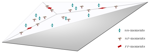
Figure 2. An illustration of coupling dofs   of $U^{2}_{1}(T^{wf})$. Here, ${\scriptscriptstyle{F\!F}}$-moments, $nn$-moments and $n{\scriptscriptstyle{F}}$-moments are associated with the dofs   (5.14a), (5.14b), and (5.14c), respectively. Note the absence of vertex or edge dofs .

Lemma 5.10.

A function $u\in{U}_{r-3}^{3}(T^{wf})$, with $r\geq 3$, is fully determined by the following dofs :

(5.15a) $$\int_{T}u\cdot\kappa, \qquad\qquad\kappa\in\mathsf{R}, \qquad\qquad{\tiny{\text{${6}\leavevmode\nobreak\ {\rm{dofs}}$}}},$$

(5.15b) $$\int_{T}u\cdot\kappa, \qquad\qquad\kappa\in\mathring{U}_{r-3}^{3}(T^{wf}), \qquad\qquad{\tiny{\text{${6r^{3}-18r^{2}+12r-6}\leavevmode\nobreak\ {\rm{dofs}}$}}}.$$

Remark 5.11.

Note that (5.15a) is equivalent to

$$\int_{T}u\cdot\kappa,\quad\kappa\in P_{\scriptscriptstyle{U}}\mathsf{R},$$

since by the definition of $L^{2}$-projection, for any $\kappa\in\mathsf{R}$,

$$\int_{T}u\cdot\kappa=\int_{T}u\cdot P_{\scriptscriptstyle{U}}\kappa,\quad\;u\in{U}_{r-3}^{3}(T^{wf}).$$

6. Commuting projections

In this section, we show that the degrees of freedom constructed in the previous sections induce projections which satisfy commuting properties.

Theorem 6.1.

Let $r\geq 3$. Let $\Pi_{r+1}^{0}:C^{\infty}(\bar{T})\otimes\mathbb{V}\rightarrow U_{r+1}^{0}(T^{wf})$ be the projection defined in Lemma 5.2, let $\Pi_{r}^{1}:C^{\infty}(\bar{T})\otimes\mathbb{V}\rightarrow U_{r}^{1}(T^{wf})$ be the projection defined in Lemma 5.8, let $\Pi_{r-2}^{2}:C^{\infty}(\bar{T})\otimes\mathbb{V}\rightarrow U_{r-2}^{2}(T^{wf})$ be the projection defined in Lemma 5.9, and let $\Pi_{r-3}^{3}:C^{\infty}(\bar{T})\otimes\mathbb{V}\rightarrow U_{r-3}^{3}(T^{wf})$ be the projection defined in Lemma 5.9. Then the following commuting properties are satisfied.

(6.1a) $$\varepsilon\big{(}\Pi_{r+1}^{0}u\big{)} =\Pi_{r}^{1}\varepsilon(u), \quad\;u\in C^{\infty}(\bar{T})\otimes\mathbb{V}$$

(6.1b) $${\rm inc}\,\Pi_{r}^{1}v =\Pi_{r-2}^{2}{\rm inc}\,v, \quad\;v\in C^{\infty}(\bar{T})\otimes\mathbb{S}$$

(6.1c) $${\rm div}\,\Pi_{r-2}^{2}w =\Pi_{r-3}^{3}{\rm div}\,w, \quad\;w\in C^{\infty}(\bar{T})\otimes\mathbb{S}$$

Proof.

(i) Proof of (6.1a): Given $u\in C^{\infty}(\bar{T})\otimes\mathbb{V}$, let $\rho=\varepsilon\big{(}\Pi_{r+1}^{0}u\big{)}-\Pi_{r}^{1}\varepsilon(u)\in U^{1}_{r}(T^{wf})$. To prove that (6.1a) holds, it suffices to show that $\rho$ vanishes on the dofs   (5.9) in Lemma 5.8. Since ${\rm inc}\,\circ\varepsilon=0$, we have dofs   of (5.9d), (5.9e), (5.9f) and (5.9k) applied to $\rho$ vanish. Next, with (5.1b), (5.1e), (5.1f), (5.1g), (5.1i) applied to $u$, and with (5.9a), (5.9g), (5.9i), (5.9j), (5.9l) applied to $\varepsilon(u)$, each term respectively imply that (5.9a), (5.9g), (5.9i), (5.9j), (5.9l) applied to $\rho$ vanish. By the identity (5.7) in Lemma 5.6, for any $\kappa\in{\rm grad}_{\scriptscriptstyle{F}}[(\mathcal{R}_{r}^{0}(F^{ct})]^{2},\text{ for all }F\in\Delta_{2}(T)$, we have:

$$\int_{\scriptscriptstyle{F}}([({\rm curl}\,\rho)^{\prime}]_{{\scriptscriptstyle{F\!F}}}-{\rm grad}_{\scriptscriptstyle{F}}(\rho_{{{\scriptscriptstyle{F}}n}}^{\perp}))\colon\kappa=\int_{\scriptscriptstyle{F}}{\rm grad}_{\scriptscriptstyle{F}}(\partial_{n}(\Pi_{r+1}^{0}u)_{\scriptscriptstyle{F}}-\partial_{n}u_{\scriptscriptstyle{F}})\colon\kappa=0,$$

where the last equality holds with (5.1h) applied to $u$. Thus, the dofs   (5.9h) applied to $\rho$ vanish. It only remains to prove that the dofs   of (5.9b), (5.9c) applied to $\rho$ vanish. To show this, we need to employ the edge-based orthonormal basis $\{n_{e}^{+},n_{e}^{-},t_{e}\}$ and write $\kappa\in{\rm sym}[\mathcal{P}_{r-2}(e)]^{3\times 3}$ as $\kappa=\kappa_{11}n_{e}^{+}(n_{e}^{+})^{\prime}+\kappa_{12}\big{(}n_{e}^{+}(n_{e}^{-})^{\prime}+n_{e}^{-}(n_{e}^{+})^{\prime}\big{)}+\kappa_{13}\big{(}n_{e}^{+}t_{e}^{\prime}+t_{e}(n_{e}^{+})^{\prime}\big{)}+\kappa_{22}n_{e}^{-}(n_{e}^{-})^{\prime}+\kappa_{23}\big{(}n_{e}^{+}(n_{e}^{-})^{\prime}+n_{e}^{-}(n_{e}^{+})^{\prime}\big{)}+\kappa_{33}t_{e}t_{e}^{\prime}$ where $\kappa_{ij}\in\mathcal{P}_{r-2}(e).$ Then,

$$\int_{e}\rho:\kappa =\int_{e}[\varepsilon(\Pi_{r+1}^{0}u)-\Pi_{r}^{1}\varepsilon(u)]:\kappa=\int_{e}\varepsilon(\Pi_{r+1}^{0}u-u):\kappa$$ by (5.9b)

$$=\int_{e}{\rm grad}\,(\Pi_{r+1}^{0}u-u):\kappa$$

$$=\int_{e}{\rm grad}\,(\Pi_{r+1}^{0}u-u)t_{e}\cdot(\kappa_{13}n_{e}^{+}+\kappa_{33}t_{e})$$ by (5.1d)

$$=\int_{e}(\Pi_{r+1}^{0}u-u)\cdot\frac{\partial}{\partial t_{e}}(\kappa_{13}n_{e}^{+}+\kappa_{33}t_{e})$$ integration by parts

$$=0 \text{by\leavevmode\nobreak\ \eqref{U0:dofa} and \eqref{U0:dofc}}.$$

Thus the dofs   of (5.9b) applied to $\rho$ vanish. Next, letting $\kappa\in[\mathcal{P}_{r-1}(e)]^{3}$, we note that

$$\int_{e}(\operatorname{curl}\rho)^{\prime}t_{e}\cdot\kappa= \int_{e}\big{[}\operatorname{curl}\varepsilon(\Pi_{r+1}^{0}u-u)\big{]}^{\prime}t_{e}\cdot\kappa\quad$$ by (5.9c)

$$= \frac{1}{2}\int_{e}\big{[}{\rm grad}\,\operatorname{curl}(\Pi_{r+1}^{0}u-u)\big{]}t_{e}\cdot\kappa\quad$$ by (2.11f)

$$= -\frac{1}{2}\int_{e}\operatorname{curl}(\Pi_{r+1}^{0}u-u)\cdot\partial_{t}\kappa\quad$$ by (5.1a) and (5.1b)

where in the last step, we have integrated by parts, and put $\partial_{t}\kappa=({\rm grad}\,\kappa)t_{e}$. The curl in the integrand above can be decomposed into terms involving $\partial_{t}(\Pi_{r+1}^{0}u-u)$ and those involving $\partial_{n_{e}^{\pm}}(\Pi_{r+1}^{0}u-u)$. The former terms can be integrated by parts yet again, which after using (5.1a), (5.1b) and (5.1c), vanish. The latter terms also vanish by (5.1d), noting that $\partial_{t}\kappa$ is of degree at most $r-2$.

(ii) Proof of (6.1b): Given $v\in C^{\infty}(\bar{T})\otimes\mathbb{S}$, let $\rho={\rm inc}\,\Pi_{r}^{1}v-\Pi_{r-2}^{2}{\rm inc}\,v\in{U}_{r-2}^{2}(T^{wf})$. To prove that (6.1b) holds, we need to show that $\rho$ vanishes on the dofs   (5.14) in Lemma 5.9. By using (5.14b) on ${\rm inc}\,v$, we have

(6.2) $$\int_{\scriptscriptstyle{F}}\rho_{nn}\kappa=\int_{\scriptscriptstyle{F}}[{\rm inc}\,(\Pi_{r}^{1}v-v)]_{nn}\kappa,\qquad\text{ for all }\kappa\in V_{r-2}^{2}(F^{ct}).$$

From (5.9e), we have that the right-hand side of (6.2) vanishes for $\kappa\in V_{r-2}^{2}(F^{ct})/\mathcal{P}_{1}(F)$. With (3.5) of Lemma 3.3, we have for any $\kappa_{1}\in\mathcal{P}_{1}(F)$,

(6.3) $$\int_{\scriptscriptstyle{F}}\rho_{nn}\kappa_{1}=\int_{\partial F}(\operatorname{curl}_{\scriptscriptstyle{F}}(\Pi_{r}^{1}v-v)_{{\scriptscriptstyle{F\!F}}})t\kappa_{1}+\int_{\partial F}(\Pi_{r}^{1}v-v)_{{\scriptscriptstyle{F\!F}}}t\cdot({\rm rot}_{\scriptscriptstyle{F}}\kappa_{1})^{\prime}.$$

By (2.11b), $\operatorname{curl}_{\scriptscriptstyle{F}}(\Pi_{r}^{1}v-v)_{{\scriptscriptstyle{F\!F}}}t\,\kappa_{1}=[\operatorname{curl}(\Pi_{r}^{1}v-v)^{\prime}]_{{{\scriptscriptstyle{F}}n}}t\,\kappa_{1}=\operatorname{curl}(\Pi_{r}^{1}v-v)^{\prime}:\kappa_{1}nt^{\prime},$ so the first term on the right-hand side of (6.3) vanishes by (5.9c). The last term in (6.3) also vanishes because

$$\int_{\partial F}(\Pi_{r}^{1}v-v)_{\scriptscriptstyle{F\!F}}t\cdot({\rm rot}_{\scriptscriptstyle{F}}\kappa_{1})^{\prime} =\int_{\partial F}Q(\Pi_{r}^{1}v-v)Qt\cdot({\rm rot}_{\scriptscriptstyle{F}}\kappa_{1})^{\prime}=\int_{\partial F}(\Pi_{r}^{1}v-v)Qt\cdot Q({\rm rot}_{\scriptscriptstyle{F}}\kappa_{1})^{\prime}$$

$$=\int_{\partial F}(\Pi_{r}^{1}v-v):{\rm sym}(Q({\rm rot}_{\scriptscriptstyle{F}}\kappa_{1})^{\prime}t)=0,$$

where we used (5.9b) in the last equality. Thus, the right-hand side of (6.3) vanishes, and therefore the right-hand side of (6.2) vanishes, i.e., the dofs   (5.14b) vanish for $\rho$.

Next using (5.14c) we have

(6.4) $$\int_{\scriptscriptstyle{F}}\rho_{{n{\scriptscriptstyle{F}}}}\cdot\kappa=\int_{\scriptscriptstyle{F}}[{\rm inc}\,(\Pi_{r}^{1}v-v)]_{{n{\scriptscriptstyle{F}}}}\cdot\kappa,\qquad\text{ for all }\kappa\in V_{{\rm div},r-2}^{1}(F^{ct}).$$

The dofs   (5.9f) imply the right-hand side of (6.4) vanishes for all $\kappa\in V_{{\rm div},r-2}^{1}(F^{ct})/\mathsf{R}(F)$. Considering $\kappa\in\mathsf{R}(F)$ in (6.4), we may conduct a similar argument as above, but now using (5.8) of Lemma 5.7, to conclude the right-hand side of (6.4) vanishes. Thus, we conclude that (5.14c) vanishes for $\rho$.

In addition, note that (5.9d) and (5.14a) imply that the dofs   (5.14a) vanish for $\rho$. Finally, the remaining dofs   of (5.14d) and (5.14e) applied to $\rho$ also vanish, thus leading to (6.1b).

(iii) Proof of (6.1c): Given $w\in C^{\infty}(\bar{T})\otimes\mathbb{S}$, let $\rho={\rm div}\,\Pi_{r-2}^{2}w-\Pi_{r-3}^{3}{\rm div}\,w\in{U}_{r-3}^{3}(T^{wf})$. To prove that (6.1c) holds, we will show that $\rho$ vanishes on the dofs   (5.15) in Lemma 5.10. Using (5.14d) and (5.15b), we have for any $\kappa\in\mathring{U}_{r-3}^{3}(T^{wf})$,

$$\int_{T}\rho\cdot\kappa=\int_{T}({\rm div}\,\Pi_{r-2}^{2}w-{\rm div}\,w)\cdot\kappa=\int_{T}({\rm div}\,w-{\rm div}\,w)\cdot\kappa=0.$$

For $\kappa\in\mathsf{R}$, we find

$$\int_{T}\rho\cdot\kappa =\int_{T}({\rm div}\,\Pi_{r-2}^{2}w-{\rm div}\,w)\cdot\kappa \text{by\leavevmode\nobreak\ }\eqref{U3:dofa}$$

$$=\int_{\partial T}(\Pi_{r-2}^{2}w-w)n_{\scriptscriptstyle{F}}\cdot\kappa$$

$$=\sum\limits_{F\in\Delta_{2}(T)}\int_{\partial F}(\Pi_{r-2}^{2}w-w)_{nn}(\kappa\cdot n_{F})-\int_{\partial F}(\Pi_{r-2}^{2}w-w)_{{n{\scriptscriptstyle{F}}}}\cdot\kappa$$

$$=0 \text{by\leavevmode\nobreak\ }\eqref{U2:dofb}\text{\leavevmode\nobreak\ and\leavevmode\nobreak\ }\eqref{U2:dofc},$$

Thus, $\rho=0$, and so the commuting property (6.1c) is satisfied. ∎

7. Global complexes

In this section, we construct the discrete elasticity complex globally by putting the local spaces together. Recall that $\Omega\subset\mathbb{R}^{3}$ is a contractible polyhedral domain, and $\mathcal{T}^{wf}_{h}$ is the Worsey-Farin refinement of the mesh $\mathcal{T}_{h}$ on $\Omega$.

We first present below the global exact de Rham complexes on Worsey-Farin splits which are needed to construct elasticity complexes; for more details, see [21, Section 6]:

(7.1a) $$0\rightarrow{\mathcal{S}}_{r}^{0}(\mathcal{T}^{wf}_{h})\xrightarrow{{\rm grad}}\mathcal{L}_{r-1}^{1}(\mathcal{T}^{wf}_{h})\xrightarrow{{\rm curl}\,}{\mathscr{V}}_{r-2}^{2}(\mathcal{T}^{wf}_{h})\xrightarrow{{\rm div}\,}{V}_{r-3}^{3}(\mathcal{T}^{wf}_{h})\rightarrow 0,$$

(7.1b) $$0\rightarrow{\mathcal{S}}_{r}^{0}(\mathcal{T}^{wf}_{h})\xrightarrow{{\rm grad}}{\mathcal{S}}_{r-1}^{1}(\mathcal{T}^{wf}_{h})\xrightarrow{{\rm curl}\,}\mathcal{L}_{r-2}^{2}(\mathcal{T}^{wf}_{h})\xrightarrow{{\rm div}\,}{\mathscr{V}}_{r-3}^{3}(\mathcal{T}^{wf}_{h})\rightarrow 0,$$

where the spaces involved are defined as follows:

$$\mathcal{S}_{r}^{0}(\mathcal{T}^{wf}_{h}) =\{q\in C^{1}(\Omega):q|_{T}\in S_{r}^{0}(T^{wf}),\,\text{ for all }T\in\mathcal{T}_{h}\},$$

$$\mathcal{S}_{r-1}^{1}(\mathcal{T}^{wf}_{h}) =\{v\in[C(\Omega)]^{3}:\operatorname{curl}v\in[C(\Omega)]^{3},\,v|_{T}\in S_{r-1}^{1}(T^{wf})\,\text{ for all }T\in\mathcal{T}_{h}\},$$

$$\mathcal{L}_{r-1}^{1}(\mathcal{T}^{wf}_{h}) =\{v\in[C(\Omega)]^{3}:v|_{T}\in{\color[rgb]{0,0,0}\mathsf{X}_{r-1}^{1}(T^{wf})},\,\text{ for all }T\in\mathcal{T}_{h}\},$$

$$\mathcal{L}_{r-2}^{2}(\mathcal{T}^{wf}_{h}) =\{w\in[C(\Omega)]^{3}:w|_{T}\in{\color[rgb]{0,0,0}\mathsf{X}_{r-2}^{2}(T^{wf})},\,\text{ for all }T\in\mathcal{T}_{h}\},$$

$$\mathscr{V}_{r-2}^{2}(\mathcal{T}^{wf}_{h}) =\{w\in H({\rm div};\Omega):w|_{T}\in V_{r-2}^{2}(T^{wf}),\,\text{ for all }T\in\mathcal{T}_{h},$$

$$\qquad{\theta_{e}(w\cdot t)=0},\,\text{ for all }e\in\mathcal{E}(\mathcal{T}^{wf}_{h})\},$$

$$\mathscr{V}_{r-3}^{3}(\mathcal{T}^{wf}_{h}) =\{p\in L^{2}(\Omega):p|_{T}\in V_{r-3}^{3}(T^{wf}),\,\text{ for all }T\in\mathcal{T}_{h},\,\theta_{e}(p)=0\text{ and }e\in\mathcal{E}(\mathcal{T}^{wf}_{h})\},$$

$$V_{r-3}^{3}(\mathcal{T}^{wf}_{h}) =\mathcal{P}_{r-3}(\mathcal{T}^{wf}_{h}),$$

and we recall $\theta_{e}(\cdot)$ is defined in (2.3). Above, these spaces are defined through their continuity requirements. They can also be defined using their local dofs  given in [21, Section 5.1 and Section 5.3]. The two definitions are proven to be equivalent in [21, Lemma 6.6 and Lemma 6.7]. We will follow a similar approach for the elasticity complex and define the global spaces in the elasticity complex in terms of their continuity requirements and show that the spaces are the same as those given through local dofs . With the global spaces defined, the global analogue of Theorem 4.4 is now given.

Theorem 7.1.

The following sequence is exact for any $r\geq 3$:

$$\begin{bmatrix}\mathcal{S}_{r+1}^{0}(\mathcal{T}^{wf}_{h})\otimes\mathbb{V}\\ \mathcal{S}_{r}^{0}(\mathcal{T}^{wf}_{h}\otimes\mathbb{V})\end{bmatrix}\xrightarrow{[{\rm grad},-{\rm mskw}\,]}\mathcal{S}_{r}^{1}(\mathcal{T}^{wf}_{h})\otimes\mathbb{V}\xrightarrow{{\rm{\rm curl}\,\Xi^{-1}{\rm curl}\,}}\mathscr{V}_{r-2}^{2}(\mathcal{T}^{wf}_{h})\otimes\mathbb{V}\xrightarrow{\left[\begin{smallmatrix}2{\rm vskw}\\ {\rm div}\,\end{smallmatrix}\right]}\begin{bmatrix}\mathscr{V}^{3}_{r-2}(\mathcal{T}^{wf}_{h})\!\otimes\!\mathbb{V}\\ V_{r-3}^{3}(\mathcal{T}^{wf}_{h})\otimes\mathbb{V}\end{bmatrix}.$$

Moreover, the kernel of the first operator is isomorphic to $\mathsf{R}$ and the last operator is surjective.

Proof.

The result follows from the exactness of the complexes (7.1a)– (7.1b), Proposition 2.1, and the exact same arguments in the proof of Theorem 4.4. ∎

Similar to the local spaces defined in Section 4.4, the global spaces involved in the elasticity complex are derived as follows:

(7.2) $$\begin{split}&U_{r+1}^{0}(\mathcal{T}^{wf}_{h})=\mathcal{S}_{r+1}^{0}(\mathcal{T}^{wf}_{h})\otimes\mathbb{V}\qquad\qquad\qquad\qquad\quad\,U_{r}^{1}(\mathcal{T}^{wf}_{h})=\{{\rm sym}(u):u\in\mathcal{S}_{r}^{1}(\mathcal{T}^{wf}_{h})\otimes\mathbb{V}\},\\ &U_{r-2}^{2}(\mathcal{T}^{wf}_{h})=\{u\in\mathscr{V}_{r-2}^{2}(\mathcal{T}^{wf}_{h})\otimes\mathbb{V}:{\rm skw}\,u=0\},\quad U_{r-3}^{3}(\mathcal{T}^{wf}_{h})=V_{r-3}^{3}(\mathcal{T}^{wf}_{h})\otimes\mathbb{V}.\end{split}$$

Theorem 7.2.

We have the following equivalent characterization of ${U}_{r}^{1}(\mathcal{T}^{wf}_{h})$:

$$U_{r}^{1}(\mathcal{T}^{wf}_{h})=\{u\in H^{1}(\Omega;\mathbb{S}): u|_{T}\in U_{r}^{1}(T^{wf}),\,\text{ for all }T\in\mathcal{T}_{h},$$

$$({\rm curl}\,u)^{\prime}\in{V}_{r-1}^{1}(\mathcal{T}^{wf}_{h})\otimes\mathbb{V},{\rm inc}(u)\in\mathscr{V}_{r-2}^{2}(\mathcal{T}^{wf}_{h})\otimes\mathbb{V}\}.$$

Proof.

This is proved similarly as the proof of Theorem 4.8 using Theorem 7.1 in place of Theorem 4.4. ∎

Now, we show that the global spaces defined in (7.2) are equivalent to those induced by the local dofs   presented in Section 5. To be more precise, we denote the global spaces induced by the local dofs   in Lemma 5.2, Lemma 5.8, Lemma 5.14 and Lemma 5.15 as $\tilde{U}_{r+1}^{0}(\mathcal{T}^{wf}_{h})$, $\tilde{U}_{r}^{1}(\mathcal{T}^{wf}_{h})$, $\tilde{U}_{r-2}^{2}(\mathcal{T}^{wf}_{h})$ and $\tilde{U}_{r-3}^{3}(\mathcal{T}^{wf}_{h})$, respectively. For example,

$$\tilde{U}_{r+1}^{0}(\mathcal{T}^{wf}_{h}):=\{u:\leavevmode\nobreak\ u|_{T}\in U_{r+1}^{0}(T^{wf}),\text{ for all }T\in\mathcal{T}^{wf}_{h},\text{ such that}$$

$$\text{the dofs\,\ \eqref{U0:dofa}-\eqref{U0:dofh} applied to $u$ from adjacent elements coincide}\}.$$

The next lemma shows that such spaces are the same as those in (7.2). Its proof is similar to [21, Lemma 6.7], so we will be brief.

Lemma 7.3.

The global spaces $\tilde{U}_{r+1}^{0}(\mathcal{T}^{wf}_{h})$, $\tilde{U}_{r}^{1}(\mathcal{T}^{wf}_{h})$, $\tilde{U}_{r-2}^{2}(\mathcal{T}^{wf}_{h})$ and $\tilde{U}_{r-3}^{3}(\mathcal{T}^{wf}_{h})$ are the same as the spaces $U_{r+1}^{0}(\mathcal{T}^{wf}_{h})$, $U_{r}^{1}(\mathcal{T}^{wf}_{h})$, $U_{r-2}^{2}(\mathcal{T}^{wf}_{h})$ and $U_{r-3}^{3}(\mathcal{T}^{wf}_{h})$, respectively.

Proof.

We only show the proof for $U_{r}^{1}(\mathcal{T}^{wf}_{h})$ as the remaining cases follow by the same reasoning. To prove that $\tilde{U}_{r}^{1}(\mathcal{T}^{wf}_{h})=U_{r}^{1}(\mathcal{T}^{wf}_{h}),$ we use the characterization of $U_{r}^{1}(\mathcal{T}^{wf}_{h})$ in Theorem 7.2. Clearly, $U_{r}^{1}(\mathcal{T}^{wf}_{h})\subset\tilde{U}_{r}^{1}(\mathcal{T}^{wf}_{h})$ since the continuity conditions in the characterization of Theorem 7.2 imply that the dofs   (5.9) applied to any $u$ in $U_{r}^{1}(\mathcal{T}^{wf}_{h})$ are single valued.

For the other direction, let function $\chi(S)$ denote the characteristic function of a simplex $S$. Let $T_{1}$ and $T_{2}$ be adjacent tetrahedra in $\mathcal{T}_{h}$ that share a face $F$. Let $K_{1}$ and $K_{2}$ be two tetrahedra in the Alfeld splits $T^{a}_{1}$ and $T^{a}_{2}$, respectively, such that $K_{1}$ and $K_{2}$ share the face $F$. Let $K^{wf}_{i}$ be the triangulation of $K_{i}$ in $\mathcal{T}^{wf}_{h}$, where $1\leq i\leq 2$. Let $u_{1}\in U_{r}^{1}(T^{wf}_{1})$ and $u_{2}\in U_{r}^{1}(T^{wf}_{2})$ such that $u_{1}$ and $u_{2}$ have the same dof values (5.9a)-(5.9j) associated with the common vertices, common edges and the triangulation $F^{\mathop{\mathrm{ct}\,}}$. Note that the natural extension of $u_{1}$ (resp., $u_{2}$) from $K_{1}^{wf}$ (resp., $K_{2}^{wf}$) to all of $K_{1}^{wf}\cup K_{2}^{wf}$ maintains its original smoothness properties across the interior faces of $K_{2}^{wf}$ (resp., $K_{1}^{wf}$). Thus, by applying the unisolvency argument in the proof of Lemma 5.8 verbatim to $w:=u_{1}-u_{2}$, we conclude that $w=0$, $(\operatorname{curl}\,w)^{\prime}_{{\scriptscriptstyle{F\!F}}}=0$, $(\operatorname{curl}\,w)^{\prime}_{{{\scriptscriptstyle{F}}n}}=0$, $({\rm inc}\,\,w)n_{{\scriptscriptstyle{F}}}=0$ and $({\rm inc}\,\,w)_{{\scriptscriptstyle{F\!F}}}=0$ on $F$. Therefore, $u:=u_{1}\chi(T_{1})+u_{2}\chi(T_{2})\in U^{1}_{r}(T^{wf}_{1}\cup T^{wf}_{2})$, and we conclude the reverse inclusion $\tilde{U}_{r}^{1}(\mathcal{T}^{wf}_{h})\subset U_{r}^{1}(\mathcal{T}^{wf}_{h}).$ ∎

Then we have the global complex summarized in the following theorem. Its proof follows along the same lines as Theorem 4.5, with Theorem 7.1 in place of Theorem 4.4.

Theorem 7.4.

The following sequence of global finite element spaces

(7.3) $$0\rightarrow\mathsf{R}\xrightarrow{\subset}{U}_{r+1}^{0}(\mathcal{T}^{wf}_{h})\xrightarrow{\varepsilon}{U}_{r}^{1}(\mathcal{T}^{wf}_{h})\xrightarrow{{\rm inc}\,}{U}_{r-2}^{2}(\mathcal{T}^{wf}_{h})\xrightarrow{{\rm div}\,}{U}_{r-3}^{3}(\mathcal{T}^{wf}_{h})\rightarrow 0$$

is a discrete elasticity complex and is exact for $r\geq 3$.

8. Conclusions

This paper constructed both local and global finite element elasticity complexes with respect to three-dimensional Worsey-Farin splits. A notable feature of the discrete spaces is the lack of extrinsic supersmoothess and accompanying dofs   at vertices in the triangulation. For example, the $H({\rm div},\mathbb{S})$-conforming space does not involve vertex or edge dofs   and is therefore conducive for hybridization. The efficient implementation of these elements with hybridization, with an emphasis on the lowest-order pair, is a subject of future work. Our results suggest that the last two pairs in the sequence (7.3) are suitable to construct mixed finite element methods for three-dimensional elasticity. However, due to the assumed regularity in Theorem 6.1, the result does not automatically yield an inf-sup stable pair. Further study of commuting projections for the pair $U_{r-2}^{2}(\mathcal{T}^{wf}_{h})\times U_{r-3}^{3}(\mathcal{T}^{wf}_{h})$ is required to prove inf-sup stability.

Appendix A Proof of Theorem 3.4

We require a few intermediate results to prove Theorem 3.4. First, we state a corollary of Theorem 3.1.

Corollary A.1.

Let $r\geq 1$. The following sequence is exact.

(A.1) $$0\ {\xrightarrow{\hskip 14.22636pt}}\ \mathring{S}_{r}^{0}(F^{\mathop{\mathrm{ct}\,}})\otimes\mathbb{V}_{2}\ \stackrel{{\scriptstyle{\rm grad}_{\scriptscriptstyle{F}}}}{{\xrightarrow{\hskip 14.22636pt}}}\ \mathring{Q}_{{\rm inc},r-1}^{1}(F^{\mathop{\mathrm{ct}\,}})\ \stackrel{{\scriptstyle\operatorname{curl}_{\scriptscriptstyle{F}}}}{{\xrightarrow{\hskip 14.22636pt}}}\ \mathring{V}_{\operatorname{curl},r-2}^{1}(F^{\mathop{\mathrm{ct}\,}})\cap\big{(}\mathring{V}_{r-2}^{2}(F^{\mathop{\mathrm{ct}\,}})\otimes\mathbb{V}_{2}\big{)}\ \xrightarrow{\hskip 14.22636pt}\ 0.$$

Proof.

This directly follows from the exactness of the sequence (3.1d). ∎

Lemma A.2.

The following sequences are exact for $r\geq 2$:

(A.2) $$\begin{bmatrix}\mathring{{S}}_{r+1}^{0}(F^{\mathop{\mathrm{ct}\,}})\otimes\mathbb{V}_{2}\\ \mathring{\mathsf{X}}_{r}^{0}(F^{\mathop{\mathrm{ct}\,}})\end{bmatrix}\xrightarrow{\begin{bmatrix}{\rm grad}_{\scriptscriptstyle{F}}&{\rm skew}\end{bmatrix}}\mathring{{Q}}_{{\rm inc},r}^{1}(F^{\mathop{\mathrm{ct}\,}})\otimes\mathbb{V}_{2}\xrightarrow{{\rm inc}_{\scriptscriptstyle{F}}}{V}_{r-2}^{2}(F^{\mathop{\mathrm{ct}\,}})\xrightarrow{\begin{bmatrix}\int_{\scriptscriptstyle{F}}^{\perp}\\ \int_{\scriptscriptstyle{F}}\end{bmatrix}}\begin{bmatrix}\mathbb{V}_{2}\\ \mathbb{R}\end{bmatrix},$$

(A.3) $$\begin{bmatrix}\mathbb{R}\\ \mathbb{V}_{2}\end{bmatrix}\xrightarrow{\begin{bmatrix}\subset&x^{\perp}\cdot\end{bmatrix}}{{S}}_{r+1}^{0}(F^{\mathop{\mathrm{ct}\,}})\xrightarrow{{\rm airy}_{\scriptscriptstyle{F}}}{{V}}_{{\rm div},r-1}^{1}(F^{\mathop{\mathrm{ct}\,}})\otimes\mathbb{V}_{2}\xrightarrow{\begin{bmatrix}{\rm skew}\\ {\rm div}_{\scriptscriptstyle{F}}\end{bmatrix}}\begin{bmatrix}{{V}}_{r-1}^{2}(F^{\mathop{\mathrm{ct}\,}})\\ {{V}}_{r-2}^{2}(F^{\mathop{\mathrm{ct}\,}})\otimes\mathbb{V}_{2}\end{bmatrix}.$$

Here, $\int_{\scriptscriptstyle{F}}^{\perp}u:=\int_{\scriptscriptstyle{F}}x^{\perp}u\leavevmode\nobreak\ dx$ with $x^{\perp}$ defined in Definition 2.2.

Proof.

Using (2.10c) and the identity $\int_{\scriptscriptstyle{F}}^{\perp}\,\operatorname{curl}_{\scriptscriptstyle{F}}\,u=\int_{\scriptscriptstyle{F}}\,\tau\,u$ for any $u\in\mathring{{V}}_{\operatorname{curl},r-1}^{1}(F^{\mathop{\mathrm{ct}\,}})$, we find that the following sequence commutes:

(A.4)

Moreover, the transpose operator $\tau$ from $\mathring{{V}}_{\operatorname{curl},r-1}^{1}(F^{\mathop{\mathrm{ct}\,}})$ to $\mathring{{V}}_{\operatorname{curl},r-1}^{1}(F^{\mathop{\mathrm{ct}\,}})$ is a bijection, and the top and bottom sequences in (A.4) are exact by Corollary A.1 and Theorem 3.1, respectively. Using the identity ${\rm inc}_{\scriptscriptstyle{F}}=\operatorname{curl}_{\scriptscriptstyle{F}}\tau\operatorname{curl}_{\scriptscriptstyle{F}}$ and Proposition 2.1, we conclude that A.2 is exact.

Likewise, using the identity ${\rm div}_{\scriptscriptstyle{F}}\,\tau\,u={\rm skew}\,{\rm rot}_{\scriptscriptstyle{F}}\,u$ for any $u\in({{\mathsf{X}}}_{r}^{0}(F^{\mathop{\mathrm{ct}\,}})\otimes\mathbb{V}_{2})$ and ${\rm rot}_{\scriptscriptstyle{F}}x^{\perp}=\tau$, we find that the following sequence commutes:

(A.5)

The top and bottom sequences in (A.5) are exact by Corollary 3.2. We then find that (A.3) is exact by Proposition 2.1, using the identity ${\rm airy}_{\scriptscriptstyle{F}}={\rm rot}_{F}\tau{\rm rot}_{F}$.

∎

Now we are ready to prove Theorem 3.4:

Proof.

(i) Proof of (3.6): from the definitions of the discrete spaces and operators, we see that (3.6) is a complex, so we only need to show exactness.

Let $v\in\mathring{Q}^{2}_{r-2}(F^{\mathop{\mathrm{ct}\,}})$. Then since $v\perp\mathcal{P}_{1}(F)$, we have $\int_{\scriptscriptstyle{F}}v=0$ and $\int_{\scriptscriptstyle{F}}^{\perp}v=0$. By the exactness of (A.2), there exists $u\in\mathring{Q}_{{\rm inc},r}^{1}(F^{\mathop{\mathrm{ct}\,}})$ such that ${\rm inc}_{\scriptscriptstyle{F}}\,u=v$. But by (2.10b), we have ${\rm inc}_{\scriptscriptstyle{F}}\,{\rm sym}\,u={\rm inc}_{\scriptscriptstyle{F}}\,u=v$. Thus we found a function $w={\rm sym}\,u\in\mathring{Q}_{{\rm inc},r}^{1,s}(F^{\mathop{\mathrm{ct}\,}})$ such that ${\rm inc}_{\scriptscriptstyle{F}}\,w=v$.

Next, let $u\in\mathring{Q}_{{\rm inc},r}^{1,s}(F^{\mathop{\mathrm{ct}\,}})$ with ${\rm inc}_{\scriptscriptstyle{F}}\,u=0$. Then $u={\rm sym}(z)$ for some $z\in\mathring{Q}_{{\rm inc},r}^{1}(F^{\mathop{\mathrm{ct}\,}})$ and ${\rm inc}_{\scriptscriptstyle{F}}\,z=0$ due to (2.10b). By exactness of (A.2), we have $z={\rm grad}_{\scriptscriptstyle{F}}w+{\rm skew}\,s$ for some $w\in\mathring{{S}}_{r+1}^{0}(F^{\mathop{\mathrm{ct}\,}})\otimes\mathbb{V}_{2}$ and $s\in\mathring{{\mathsf{X}}}_{r}^{0}(F^{\mathop{\mathrm{ct}\,}})$. Then $u={\rm sym}(z)=\varepsilon_{\scriptscriptstyle{F}}(w)-{\rm sym}({\rm skew}\,s)=\varepsilon_{\scriptscriptstyle{F}}(w)$.

(ii) Proof of (3.7): again, it is easy to see that (3.7) is a complex, so we only need to show exactness.

Let $v\in V^{2}_{r-3}(F^{\mathop{\mathrm{ct}\,}})\otimes\mathbb{V}_{2}$. Then by the exactness of (A.3), we have $u\in{{V}}_{{\rm div},r-2}^{1}(F^{\mathop{\mathrm{ct}\,}})\otimes\mathbb{V}_{2}$ such that ${\rm div}_{\scriptscriptstyle{F}}\,u=v$ and ${\rm skew}\,u=0$ and thus making $u\in Q^{1}_{r-2}(F^{\mathop{\mathrm{ct}\,}})$.

Next, let $u\in Q^{1}_{r-2}(F^{\mathop{\mathrm{ct}\,}})$ with ${\rm div}_{\scriptscriptstyle{F}}\,u=0$. Then again using (A.3) and ${\rm skew}\,u=0$, there exists $z\in{{S}}_{r}^{0}(F^{\mathop{\mathrm{ct}\,}})$ such that ${\rm airy}_{\scriptscriptstyle{F}}\,z=u$.

Finally, for any $u\in{{S}}_{r}^{0}(F^{\mathop{\mathrm{ct}\,}})$ with ${\rm airy}_{\scriptscriptstyle{F}}\,u=0$, we have $u=w+x^{\perp}\cdot s$ for some $w\in\mathbb{R}$, $s\in\mathbb{V}_{2}$, and $x$ a point on the face $F$. Therefore, $u\in\mathcal{P}_{1}(F)$.

∎

Appendix B Proof of Lemma 4.6

Proof.

We first show that $\dim P_{\scriptscriptstyle{U}}\mathsf{R}=\dim\mathsf{R}=6$. This follows if we show that the kernel of $P_{U}$ is empty. Let $v\in\mathsf{R}$ and assume that $P_{\scriptscriptstyle{U}}v=0$. Then, by the definition of $P_{\scriptscriptstyle{U}}$ and the fact that $v$ is a linear function, we must have that $v$ vanishes on the barycenter of each $K\in T^{wf}$. This implies that $v\equiv 0$ if there are three such barycenters that are not collinear. To see that there are such barycenters, recall that the barycenter of $K\in T^{wf}$ is the average of the four vertices of $K$. Hence the line connecting barycenters of two adjacent $K_{\pm}\in T^{wf}$ is parallel to the line connecting the two vertices opposite to the common face $F=\partial K_{+}\cap\partial K_{-}$. Thus taking, for example, three subtetrahedra in $T^{wf}$ with a face contained in a common $F\in\Delta_{2}(\mathcal{T}_{h})$, we see that their barycenters cannot be collinear, since no three of their vertices are collinear.

We now prove (4.9). Since $\dim\mathsf{R}=6$ and by the definition of $\mathring{U}_{0}^{3}(T^{wf})$, we have

$$\dim\mathring{U}_{0}^{3}(T^{wf})\geq\dim{U}_{0}^{3}(T^{wf})-\dim\mathsf{R}=36-6=30.$$

We use that

$${U}_{0}^{3}(T^{wf})=\mathring{U}_{0}^{3}(T^{wf})\oplus[\mathring{U}_{0}^{3}(T^{wf})]^{\perp},$$

and obtain $\dim[\mathring{U}_{0}^{3}(T^{wf})]^{\perp}\leq 6$. However, one can easily show that $P_{\scriptscriptstyle{U}}\mathsf{R}\subset[\mathring{U}_{0}^{3}(T^{wf})]^{\perp}$ which implies $\dim[\mathring{U}_{0}^{3}(T^{wf})]^{\perp}=6$ and $P_{\scriptscriptstyle{U}}\mathsf{R}=[\mathring{U}_{0}^{3}(T^{wf})]^{\perp}$.

∎

Appendix C Proof of Lemma 5.3

Proof.

Fix $F\in\Delta_{2}(T)$, and let $e\in\Delta_{1}^{I}(F^{ct})$ be an internal edge in the induced Clough-Tocher split of $F$. Let $f$ be the corresponding internal face of $T^{wf}$ with $e$ as an edge, and let $n_{f}$ is a unit-normal to $f$. We further set $t_{e}$ to be a unit tangent vector to $e$ and $s_{e}=n_{F}\times t_{e}$ to be a unit tangent vector of $F$ orthogonal to $t_{e}$.

Since $n_{f}\cdot t_{e}=0$, we have $n_{f}=(n_{f}\cdot n_{\scriptscriptstyle{F}})n_{\scriptscriptstyle{F}}+(n_{f}\cdot s_{e})s_{e}$. Since $\sigma\in V_{r}^{2}(T^{wf})\otimes\mathbb{V}$, we have $\sigma n_{f}$ is single-valued on $e$ and hence, by symmetry of $\sigma$, $(\sigma\ell)\cdot n_{f}$ is single-valued on $e$. Therefore, on $e$, with $(\sigma\ell)\cdot n_{\scriptscriptstyle{F}}=n_{\scriptscriptstyle{F}}^{\prime}\sigma\ell=0$, we have $(\sigma\ell)\cdot n_{f}=(n_{f}\cdot s_{e})(\sigma\ell)\cdot s_{e}$ and so $[\![{\sigma_{{\scriptscriptstyle{F}}\ell}\cdot s_{e}}]\!]_{e}=[\![{(\sigma\ell)\cdot s_{e}}]\!]_{e}=0$ for any $e\in\Delta_{1}^{I}(F^{ct})$. Therefore, $\sigma_{{\scriptscriptstyle{F}}\ell}\in V_{{\rm div},r}^{1}(F^{\mathop{\mathrm{ct}\,}})$ on each $F\in\Delta_{2}(T)$. ∎

Appendix D Proof of Lemma 5.4

Proof.

Since $w\in V^{1}_{r-1}(T^{wf})\otimes\mathbb{V}$ and $w^{\prime}\in V^{2}_{r-1}(T^{wf})\otimes\mathbb{V}$, then $n_{f}^{\prime}w$, $wt_{e}$ and $wt_{s}$ are continuous cross $e$ on $F$:

(D.1) $$[\![{n_{f}^{\prime}w}]\!]_{e}=0,\quad[\![{wt_{e}}]\!]_{e}=0,\quad[\![{wt_{s}}]\!]_{e}=0.$$

Let $s_{e}=\alpha_{1}n_{f}+\beta_{1}t_{s}$, $n_{\scriptscriptstyle{F}}=\alpha_{2}n_{f}+\beta_{2}t_{s}$, and note $\alpha_{1}\neq 0$ and $\beta_{2}\neq 0$.

Since $n_{\scriptscriptstyle{F}}^{\prime}wQ|_{F}=0$, for any $e\in\Delta_{1}^{I}(F^{ct})$,

$$0=[\![{n_{\scriptscriptstyle{F}}^{\prime}ws_{e}}]\!]_{e} =[\![{(\alpha_{2}n_{f}^{\prime}+\beta_{2}t_{s}^{\prime})w(\alpha_{1}n_{f}+\beta_{1}t_{s})}]\!]_{e}$$

$$=\alpha_{1}\alpha_{2}[\![{n_{f}^{\prime}wn_{f}}]\!]_{e}+\alpha_{2}\beta_{1}[\![{n_{f}^{\prime}wt_{s}}]\!]_{e}+\alpha_{1}\beta_{2}[\![{t_{s}^{\prime}wn_{f}}]\!]_{e}+\beta_{2}\beta_{1}[\![{t_{s}^{\prime}wt_{s}}]\!]_{e}$$

$${=\alpha_{1}\beta_{2}[\![{t_{s}^{\prime}wn_{f}}]\!]_{e}.}$$

Thus, we have

$$[\![{t_{s}^{\prime}wn_{f}}]\!]_{e}=0,$$

and therefore

$$[\![{s_{e}^{\prime}ws_{e}}]\!]_{e}=\alpha_{1}^{2}[\![{n_{f}^{\prime}wn_{f}}]\!]_{e}+\alpha_{1}\beta_{1}[\![{n_{f}^{\prime}wt_{s}}]\!]_{e}+\alpha_{1}\beta_{1}[\![{t_{s}^{\prime}wn_{f}}]\!]_{e}+\beta_{1}^{2}[\![{t_{s}^{\prime}wt_{s}}]\!]_{e}=0.$$

We have $[\![{t_{e}^{\prime}wn_{f}}]\!]_{e}=0$ since $w_{{\scriptscriptstyle{F\!F}}}=0$ and

$$0=[\![{t_{e}^{\prime}ws_{e}}]\!]_{e}=[\![{t_{e}^{\prime}w(\alpha_{1}n_{f}+\beta_{1}t_{s})}]\!]_{e}=\alpha_{1}[\![{t_{e}^{\prime}wn_{f}}]\!]_{e}+\beta_{1}[\![{t_{e}^{\prime}wt_{s}}]\!]_{e}{=\alpha_{1}[\![{t_{e}^{\prime}wn_{f}}]\!]_{e}},$$

where we use (D.1). This implies that

$$[\![{t_{e}^{\prime}wn_{\scriptscriptstyle{F}}}]\!]_{e}=0$$

since

$$[\![{t_{e}^{\prime}wn_{\scriptscriptstyle{F}}}]\!]_{e}=[\![{t_{e}^{\prime}w(\alpha_{2}n_{f}+\beta_{2}t_{s})}]\!]_{e}=0.$$

∎

Appendix E Proof of Lemma 5.5

Proof.

Write $\ell=a_{1}t_{1}+a_{2}t_{2}$, $m=a_{1}t_{2}-a_{2}t_{1}$, where $t_{1},t_{2}$ are tangential basis defined in Section 2.3. We also set $t_{3}=n_{\scriptscriptstyle{F}}$, and write $u=\sum\limits_{i,j=1}^{3}u_{ij}t_{i}t_{j}^{\prime}$. We then have the following identities for the components of ${\rm curl}\,u$ ($s\in\{1,2,3\})$:

(E.1) $$\begin{split}t_{s}^{\prime}({\rm curl}\,u)t_{1}&=\partial_{t_{2}}u_{s3}-\partial_{t_{3}}u_{s2},\\ t_{s}^{\prime}({\rm curl}\,u)t_{2}&=\partial_{t_{3}}u_{s1}-\partial_{t_{1}}u_{s3},\\ t_{s}^{\prime}({\rm curl}\,u)t_{3}&=\partial_{t_{1}}u_{s2}-\partial_{t_{2}}u_{s1}.\end{split}$$

We then compute

(E.2) $$\begin{split}\ell^{\prime}({\rm curl}\,u)m&=(a_{1}t_{1}+a_{2}t_{2})^{\prime}({\rm curl}\,u)(a_{1}t_{2}-a_{2}t_{1})\\ &=(a_{1})^{2}(\partial_{t_{3}}u_{11}-\partial_{t_{1}}u_{13})-(a_{2})^{2}(\partial_{t_{2}}u_{23}-\partial_{t_{3}}u_{22})\\ &\qquad+a_{1}a_{2}(\partial_{t_{3}}u_{21}-\partial_{t_{1}}u_{23}-\partial_{t_{2}}u_{13}+\partial_{t_{3}}u_{12})\\ &=\partial_{t_{3}}((a_{1})^{2}u_{11}+(a_{2})^{2}u_{22}+a_{1}a_{2}(u_{21}+u_{12}))\\ &\qquad-a_{1}(a_{2}\partial_{t_{2}}u_{13}+a_{1}\partial_{t_{1}}u_{13})-a_{2}(a_{1}\partial_{t_{1}}u_{23}+a_{2}\partial_{t_{2}}u_{23})\\ &=\partial_{t_{3}}(\ell^{\prime}u_{{\scriptscriptstyle{F\!F}}}\ell)-a_{1}\partial_{\ell}u_{13}-a_{2}\partial_{\ell}u_{23}\\ &=\partial_{n}(\ell^{\prime}u_{{\scriptscriptstyle{F\!F}}}\ell)-\partial_{l}(u_{{{\scriptscriptstyle{F}}n}}\cdot\ell)=\partial_{n}(\ell^{\prime}u_{{\scriptscriptstyle{F\!F}}}\ell)-{\rm grad}_{\scriptscriptstyle{F}}(u_{{{\scriptscriptstyle{F}}n}}\cdot\ell)\cdot\ell.\end{split}$$

Similarly, by using (E.1), we have

(E.3) $$\begin{split}\ell^{\prime}({\rm curl}\,u)\ell&=(a_{1}t_{1}+a_{2}t_{2})^{\prime}({\rm curl}\,u)(a_{1}t_{1}+a_{2}t_{2})\\ &=(a_{1})^{2}(\partial_{t_{2}}u_{13}-\partial_{t_{3}}u_{12})+(a_{2})^{2}(\partial_{t_{3}}u_{21}-\partial_{t_{1}}u_{23})\\ &\qquad+a_{1}a_{2}(\partial_{t_{2}}u_{23}-\partial_{t_{3}}u_{22}+\partial_{t_{3}}u_{11}-\partial_{t_{1}}u_{13})\\ &=\partial_{t_{3}}(-(a_{1})^{2}u_{12}+(a_{2})^{2}u_{21}+a_{1}a_{2}(u_{11}-u_{22}))\\ &\qquad-a_{1}(-a_{1}\partial_{t_{2}}u_{13}+a_{2}\partial_{t_{1}}u_{13})+a_{2}(a_{1}\partial_{t_{2}}u_{23}-a_{2}\partial_{t_{1}}u_{23})\\ &=-\partial_{t_{3}}(m^{\prime}u_{{\scriptscriptstyle{F\!F}}}\ell)+a_{1}\partial_{m}u_{13}+a_{2}\partial_{m}u_{23}\\ &=-\partial_{n}(m^{\prime}u_{{\scriptscriptstyle{F\!F}}}\ell)+\partial_{m}(u_{{{\scriptscriptstyle{F}}n}}\cdot\ell)=-\partial_{n}(m^{\prime}u_{{\scriptscriptstyle{F\!F}}}\ell)+{\rm grad}_{\scriptscriptstyle{F}}(u_{{{\scriptscriptstyle{F}}n}}\cdot\ell)\cdot m.\end{split}$$

Finally, again by using (E.1), we have

(E.4) $$\begin{split}n_{F}^{\prime}({\rm curl}\,u)\ell&=t_{3}^{\prime}({\rm curl}\,u)(a_{1}t_{1}+a_{2}t_{2})\\ &=(a_{1}\partial_{t_{2}}u_{33}-a_{2}\partial_{t_{1}}u_{33})+\partial_{t_{3}}(a_{2}u_{31}-a_{1}a_{32})\\ &=\partial_{m}u_{33}-\partial_{n}(u_{n{\scriptscriptstyle{F}}}\cdot m)=({\rm grad}_{F}u_{33})\cdot m-\partial_{n}(u_{n{\scriptscriptstyle{F}}}\cdot m).\end{split}$$

Lemma 5.5 now follows from (E.2)–(E.4) and the first case in Lemma 5.1. ∎

Appendix F Proof of Lemma 5.6

Proof.

(i) Continuity: we show the continuity of $w_{{\scriptscriptstyle{F\!F}}}-{\rm grad}_{\scriptscriptstyle{F}}{\color[rgb]{0,0,0}u_{n{\scriptscriptstyle{F}}}^{\perp}}$. Recall the notation from Section 2.2. Since $w\in V^{1}_{r-1}(T^{wf})\otimes\mathbb{V}$ (by Theorem 4.8), for any $e\in\Delta_{1}^{I}(F^{ct})$ we have $[\![{w_{{\scriptscriptstyle{F\!F}}}t_{e}}]\!]_{e}=0$ due to $[\![{wt_{e}}]\!]_{e}=0$. Consequently, because $u$ is continuous, we have

(F.1) $$[\![{(w_{{\scriptscriptstyle{F\!F}}}-{\rm grad}_{\scriptscriptstyle{F}}{\color[rgb]{0,0,0}u_{n{\scriptscriptstyle{F}}}^{\perp}})t_{e}}]\!]_{e}=0.$$

Now to prove the continuity of $w_{{\scriptscriptstyle{F\!F}}}-{\rm grad}_{\scriptscriptstyle{F}}{\color[rgb]{0,0,0}u_{n{\scriptscriptstyle{F}}}^{\perp}}$ on $F$, it suffices to prove $[\![{(w_{{\scriptscriptstyle{F\!F}}}-{\rm grad}_{\scriptscriptstyle{F}}{\color[rgb]{0,0,0}u_{n{\scriptscriptstyle{F}}}^{\perp}})s_{e}}]\!]_{e}=0$ for all $e\in\Delta^{I}_{1}(F^{ct})$. Using $w^{\prime}\in V^{2}_{r-1}(T^{wf})\otimes\mathbb{V}$ and $w_{Fn}=0$, by Lemma 5.4 we have

(F.2) $$[\![{s_{e}^{\prime}w_{{\scriptscriptstyle{F\!F}}}s_{e}}]\!]_{e}=[\![{s_{e}^{\prime}ws_{e}}]\!]_{e}=0.$$

Next we show that $[\![{s_{e}^{\prime}{\rm grad}_{\scriptscriptstyle{F}}({\color[rgb]{0,0,0}u_{n{\scriptscriptstyle{F}}}^{\perp}})s_{e}}]\!]_{e}=0$ and $[\![{t_{e}^{\prime}(w_{{\scriptscriptstyle{F\!F}}}-{\color[rgb]{0,0,0}u_{n{\scriptscriptstyle{F}}}^{\perp}})s_{e}}]\!]_{e}=0$. Since $u\in\mathsf{X}_{r}^{1}(T^{wf})\otimes\mathbb{V}$ and $u_{{\scriptscriptstyle{F\!F}}}=0$ on $F$, we have

$$[\![{s_{e}^{\prime}{\rm grad}_{\scriptscriptstyle{F}}({\color[rgb]{0,0,0}u_{n{\scriptscriptstyle{F}}}^{\perp}})s_{e}}]\!]_{e} =[\![{{\rm grad}_{\scriptscriptstyle{F}}({\color[rgb]{0,0,0}u_{n{\scriptscriptstyle{F}}}^{\perp}}\cdot s_{e})\cdot s_{e}}]\!]_{e}=[\![{{\rm grad}_{\scriptscriptstyle{F}}(u_{{{\scriptscriptstyle{F}}n}}^{\perp}\cdot s_{e})\cdot s_{e}}]\!]_{e}$$

(F.3) $$=[\![{{\rm grad}_{\scriptscriptstyle{F}}(u_{{{\scriptscriptstyle{F}}n}}\cdot t_{e})\cdot s_{e}}]\!]_{e}=-[\![{t_{e}^{\prime}({\rm curl}\,u)^{\prime}t_{e}}]\!]_{e}=0,$$

where the third equality comes from (2.6) and the fourth equality uses (5.5) in Lemma 5.5 with $\ell=t_{e}$ and $m=s_{e}$. Similarly by (5.4) in Lemma 5.5 with $\ell=s_{e}$, $m=-t_{e}$ and (2.6), we have $[\![{t_{e}^{\prime}{\rm grad}_{\scriptscriptstyle{F}}({\color[rgb]{0,0,0}u_{n{\scriptscriptstyle{F}}}^{\perp}})s_{e}}]\!]_{e}=[\![{t_{e}^{\prime}({\rm curl}\,u)^{\prime}s_{e}}]\!]_{e}$. Therefore, we have

(F.4) $$[\![{t_{e}^{\prime}(w_{{\scriptscriptstyle{F\!F}}}-{\rm grad}_{F}{\color[rgb]{0,0,0}u_{n{\scriptscriptstyle{F}}}^{\perp}})s_{e}}]\!]_{e}=[\![{t_{e}^{\prime}[({\rm curl}\,u)^{\prime}]_{{\scriptscriptstyle{F\!F}}}s_{e}}]\!]_{e}-[\![{t_{e}^{\prime}({\rm curl}\,u)^{\prime}s_{e}}]\!]_{e}=0.$$

Combining (F.1), (F.2), (F) and (F.4), we conclude that $w_{{\scriptscriptstyle{F\!F}}}-{\rm grad}_{\scriptscriptstyle{F}}{\color[rgb]{0,0,0}u_{n{\scriptscriptstyle{F}}}^{\perp}}$ is continuous on $F$.

(ii) Proof of (5.7): With (2.11g), (2.11h) and (2.5), we have

$$2w_{{\scriptscriptstyle{F\!F}}}={\rm grad}_{\scriptscriptstyle{F}}({\rm grad}_{\scriptscriptstyle{F}}(v\cdot n_{\scriptscriptstyle{F}})\times n_{\scriptscriptstyle{F}}-(\partial_{n}v_{\scriptscriptstyle{F}})\times n_{\scriptscriptstyle{F}}).$$

Then with (2.11i), (2.11j) and (2.6), we obtain

$$2{\rm grad}_{\scriptscriptstyle{F}}u_{{n{\scriptscriptstyle{F}}}}^{\perp}=2{\rm grad}_{\scriptscriptstyle{F}}[(\varepsilon(v))_{{n{\scriptscriptstyle{F}}}}]^{\perp}={\rm grad}_{\scriptscriptstyle{F}}({\rm grad}_{\scriptscriptstyle{F}}(v\cdot n_{\scriptscriptstyle{F}})\times n_{\scriptscriptstyle{F}}+(\partial_{n}v_{\scriptscriptstyle{F}})\times n_{\scriptscriptstyle{F}}).$$

Therefore, by computing the difference of the above two equations, we conclude that $w_{{\scriptscriptstyle{F\!F}}}-{\rm grad}_{\scriptscriptstyle{F}}u_{{n{\scriptscriptstyle{F}}}}^{\perp}={\rm grad}_{\scriptscriptstyle{F}}(\partial_{n}v_{\scriptscriptstyle{F}}\times n_{\scriptscriptstyle{F}}).$ ∎

References

- [1] S. Adams and B. Cockburn, A mixed finite element method for elasticity in three dimensions, Journal of Scientific Computing, 25 (2005), pp. 515–521.
- [2] D. Arnold, G. Awanou, and R. Winther, Finite elements for symmetric tensors in three dimensions, Mathematics of Computation, 77 (2008), pp. 1229–1251.
- [3] D. N. Arnold, J. Douglas, and C. P. Gupta, A family of higher order mixed finite element methods for plane elasticity, Numerische Mathematik, 45 (1984), pp. 1–22.
- [4] D. N. Arnold, R. S. Falk, and R. Winther, Finite element exterior calculus,homological techniques, and applications, Acta Numerica, (2006), pp. 1–155.
- [5] D. N. Arnold and K. Hu, Complexes from complexes, Foundations of Computational Mathematics, 21 (2021), pp. 1739–1774.
- [6] D. N. Arnold and J. Qin, Quadratic velocity/linear pressure Stokes elements, Advances in computer methods for partial differential equations, 7 (1992), pp. 28–34.
- [7] D. N. Arnold and R. Winther, Mixed finite elements for elasticity, Numerische Mathematik, 92 (2002), pp. 401–419.
- [8] D. Boffi, F. Brezzi, L. F. Demkowicz, R. G. Durán, R. S. Falk, M. Fortin, and R. S. Falk, Finite element methods for linear elasticity, Mixed Finite Elements, Compatibility Conditions, and Applications: Lectures given at the CIME Summer School held in Cetraro, Italy June 26–July 1, 2006, (2008), pp. 159–194.
- [9] F. Bonizzoni, K. Hu, G. Kanschat, and D. Sap, Discrete tensor product bgg sequences: splines and finite elements, arXiv preprint arXiv:2302.02434, (2023).
- [10] A. Čap, J. Slovák, and V. Souček, Bernstein-Gelfand-Gelfand sequences, Annals of Mathematics, 154 (2001), pp. 97–113.
- [11] L. Chen and X. Huang, Complexes from complexes: Finite element complexes in three dimensions, arXiv preprint arXiv:2211.08656, (2022).
- [12] , A finite element elasticity complex in three dimensions, Mathematics of Computation, 91 (2022), pp. 2095–2127.
- [13] S. H. Christiansen, J. Gopalakrishnan, J. Guzmán, and K. Hu, A discrete elasticity complex on three-dimensional Alfeld splits, arXiv preprint arXiv:2009.07744, (2020).
- [14] S. H. Christiansen and K. Hu, Generalized finite element systems for smooth differential forms and stokes’ problem, Numerische Mathematik, 140 (2018), pp. 327–371.
- [15] , Finite element systems for vector bundles: elasticity and curvature, Foundations of Computational Mathematics, (2022), pp. 1–52.
- [16] R. W. Clough, Finite element stiffness matricess for analysis of plate bending, in Proc. of the First Conf. on Matrix Methods in Struct. Mech., 1965, pp. 515–546.
- [17] F. Dassi, C. Lovadina, and M. Visinoni, A three-dimensional Hellinger–Reissner virtual element method for linear elasticity problems, Computer Methods in Applied Mechanics and Engineering, 364 (2020), p. 112910.
- [18] M. Eastwood, A complex from linear elasticity, in Proceedings of the 19th Winter School” Geometry and Physics”, Circolo Matematico di Palermo, 2000, pp. 23–29.
- [19] G. Fu, J. Guzmán, and M. Neilan, Exact smooth piecewise polynomial sequences on Alfeld splits, Math. Comp., 89 (2020), pp. 1059–1091.
- [20] J. Guzmán, A. Lischke, and M. Neilan, Exact sequences on Powell–Sabin splits, Calcolo, 57 (2020), pp. 1–25.
- [21] J. Guzmán, A. Lischke, and M. Neilan, Exact sequences on Worsey-Farin splits, Math. Comp., 91 (2022), pp. 2571–2608.
- [22] J. Guzmán and M. Neilan, Symmetric and conforming mixed finite elements for plane elasticity using rational bubble functions, Numerische Mathematik, 126 (2014), pp. 153–171.
- [23] J. Hu and S. Zhang, A family of symmetric mixed finite elements for linear elasticity on tetrahedral grids, Science China Mathematics, 58 (2015), pp. 297–307.
- [24] M.-J. Lai and L. L. Schumaker, Spline functions on triangulations, vol. 110, Cambridge University Press, 2007.
- [25] A. Lischke, Exact smooth piecewise polynomials on Powell–Sabin and Worsey–Farin splits, PhD thesis, Division of Applied Mathematics, Brown University, 2020.
- [26] MFO, Oberwolfach Reports, no. MFO Workshop 2225, MFO, 2022. Workshop on “Hilbert Complexes: Analysis, Applications, and Discretizations” held 19 Jun – 25 Jun 2022. https://doi.org/10.14760/OWR-2022-29.
- [27] J.-C. Nédélec, Mixed finite elements in , Numerische Mathematik, 35 (1980), pp. 315–341.
- [28] A. Worsey and G. Farin, An n-dimensional Clough-Tocher interpolant, Constructive Approximation, 3 (1987), pp. 99–110.