SplitOut: Out-of-the-Box Training-Hijacking Detection in Split Learning via Outlier Detection

Abstract

Split learning enables efficient and privacy-aware training of a deep neural network by splitting a neural network so that the clients (data holders) compute the first layers and only share the intermediate output with the central compute-heavy server. This paradigm introduces a new attack medium in which the server has full control over what the client models learn, which has already been exploited to infer the private data of clients and to implement backdoors in the client models. Although previous work has shown that clients can successfully detect such training-hijacking attacks, the proposed methods rely on heuristics, require tuning of many hyperparameters, and do not fully utilize the clients’ capabilities. In this work, we show that given modest assumptions regarding the clients’ compute capabilities, an out-of-the-box outlier detection method can be used to detect existing training-hijacking attacks with almost-zero false positive rates. We conclude through experiments on different tasks that the simplicity of our approach we name SplitOut makes it a more viable and reliable alternative compared to the earlier detection methods.

1 Introduction

Neural networks often perform better when they are trained on more data using more parameters, which in turn requires more computational resources. However, the required computing resources might be inaccessible in many application scenarios, and it is not always possible to share data freely in fields such as healthcare [2, 35].

Distributed and/or outsourced deep learning frameworks such as split learning [53, 20] and federated learning [5, 29] aim to solve these problems by enabling a group of resource-constrained data holders (clients) to collaboratively train a neural network on their collective data without explicitly sharing private data, and also while offloading a (large) share of computational load to more resourceful servers.

In split learning, a neural network is split into two parts, with the clients computing the first few layers on their private input and sharing the output with the central server, who then computes the rest of the layers. In federated learning, each client computes the full network locally, then their parameter updates are aggregated at a central server, and the aggregated update is shared across the clients. While both of these systems can indeed utilize the collective data set of the clients without raw data sharing, they have been shown to leak information about private data in many different ways [14, 36, 17, 15, 66, 16].

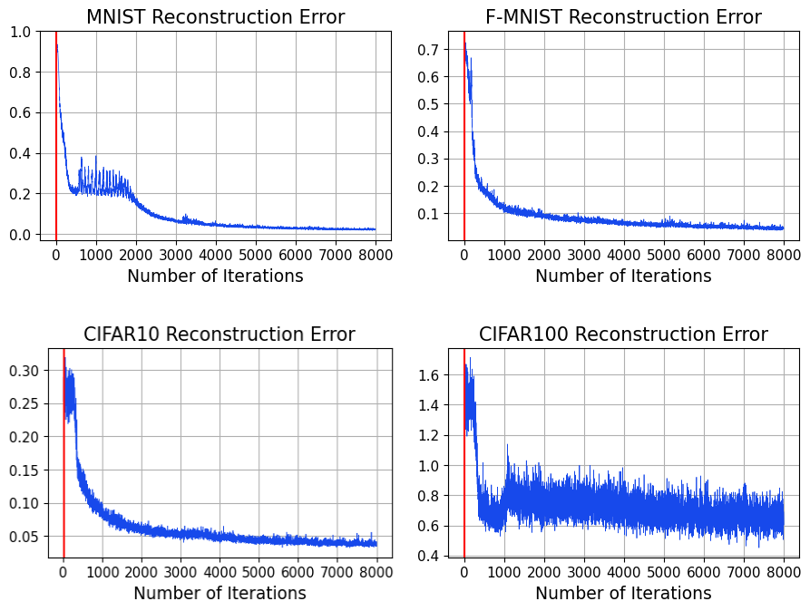
Figure 1: Image reconstruction errors of training-hijacking attack (specifically FSHA [36]) for 4 different datasets. The red line represents the point SplitOut detects the attack, well before the attack converges.

The Problem. What a split learning client learns is fully determined by the server, since the clients’ parameter updates are propagated back from the gradients the server sends. A malicious server can thus launch training-hijacking attacks that have been shown to be effective in inferring clients’ private data [36, 16] and implementing backdoors in the client models [65]. Nevertheless, since training is an iterative process, clients can potentially detect training-hijacking attacks and stop training before the attack converges. Two such detection methods have been proposed in earlier work: an active method that relies on the clients tampering with the data to observe the resulting changes in the system [13], and a passive method that depends only on observing the system [16], motivated by the fact that active methods can be detected and circumvented by the attacker. Both of these methods primarily rely on heuristic approaches that do not fully utilize the clients’ capabilities, which motivates the search for less fragile and simpler-to-use approaches.

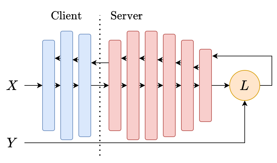
(a) With label-sharing.

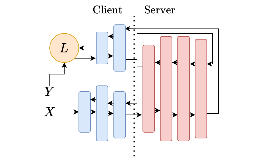
(b) Without label-sharing.

Figure 2: Potential SplitNN setups. Arrows denote the forward and backward passes, starting with the input data $X$, and propagating backwards after the loss computation using the labels $Y$. In Figure 2(a), clients send the labels to the server along with the intermediate outputs. In Figure 2(b), the model terminates on the client side, and thus the clients do not share their labels.

Our Contribution. In this work, we show that given modest assumptions on the clients’ compute capabilities, an out-of-the-box outlier detection algorithm can successfully distinguish the gradients sent by a malicious training-hijacking server from those sent by an honest one with almost perfect accuracy, resulting in a simple-yet-effective passive detection method. We empirically demonstrate the effectiveness of the method against the existing training-hijacking attacks [36, 65, 16] and an adaptive attacker that can bypass the active method of [13]. Through the data we collected as part of the experiments, we discover that the differences between the honest training and training-hijacking optimization processes result in training-hijacking gradients having significantly distinguishable neighborhood characteristics compared to honest gradients, which makes the use of the neighborhood-based local outlier factor outlier detection algorithm [6] that can be used out-of-the-box from popular frameworks [39] highly effective. Due to the proactive design of our solution, we think that it can potentially detect some not-yet-known attacks, rather than taking a reactive approach.

We will make the model architectures and training code to reproduce the experiments we report in the paper publicly available.

2 Background and Motivation

2.1 Neural Networks and Data Privacy

Modern machine learning (ML) methods employ the principle of empirical risk minimization [48], where given a dataset $\mathcal{D}=\{(x_{i},y_{i})\}_{i=1}^{N}$ and a space $\mathcal{F}$ of functions parameterized via $\theta$, the goal is to find $\theta^{*}$ which minimizes some loss $\mathcal{L}(f_{\theta},\mathcal{D})$. Many modern systems utilize variants of the iterative stochastic gradient descent (SGD) method, where parameters are updated by sampling a mini-batch $\mathcal{B}\subset\mathcal{D}$ and taking a step in the direction of steepest descent on the loss landscape. In the most basic setting, the update is controlled by the learning rate $\alpha$, such that $\theta^{t+1}\leftarrow\theta^{t}-\alpha\cdot\nabla_{\theta}\mathcal{L}(f_{\theta},\mathcal{B})$.

Neural networks [43] define a certain kind of function space. In its simplest form, each neuron in a neural network layer computes a weighted sum of the previous layer neurons and applies a non-linear activation, such as the sigmoid function. Single-layer neural networks defined in this way are universal approximators [23] provided they are wide enough; however, stacking narrower layers to build deep neural networks (DNNs) leads to more efficient training for the same number of parameters. Practical training of DNNs was made possible by the backpropagation algorithm [44], in which a DNN is treated as a composition of functions and the gradient $\nabla_{\theta}\mathcal{L}$ is decomposed via the chain rule, starting with the final layer and flowing backwards through the network (see e.g. [19] for a definitive treatment of these issues).

Although such defined fully-connected DNNs are highly expressive, this expressivity results in huge search spaces that are difficult to optimize. Instead, the function space is restricted through inductive biases that make assumptions about the structure of the data, such as using convolutional neural networks [31] that are invariant to translations of the features (e.g. edges in images), graph neural networks [28, 52] that are invariant to the order in which the nodes of the graph are processed, or attention-based transformers [49, 11] that are designed to process sequential data such as text. The recent framework of geometric deep learning [7] attempts to formalize these principles.

The effectiveness of these specialized model architectures, along with access to ever more data and compute resources has gradually led to ground-breaking performance in tasks such as language modeling [8] and image generation [42]. This has in turn caused the research community to consider ML systems in a more holistic way, focusing e.g. on their safety [22] and energy use [38], but most importantly for our purposes, data privacy.

Data privacy concerns and DNNs relate in two ways: 1) DNNs often perform better given more data, yet privacy regulations in fields such as healthcare [2, 35] make it difficult to utilize existing data, and 2) neural networks, being the black-boxes they are, can leak training or input data [9, 15]. Such data leakage (see Section 5 for more examples) has led to discussions around whether ML models should be classified as personal data of those whose data was used to train the models [50], and data privacy has been featured as a key concern in very recent regulatory work on artificial intelligence (AI) such as the Blueprint for an AI Bill of Rights published by the US Government [58] and the EU AI Act [51]. Attempts to enable privacy-aware training have resulted in frameworks such as split learning which we focus on next.

2.2 Split Learning

Split learning (SplitNN) [20, 55, 53] aims to address two challenges: 1) data-sharing in sensitive fields such as healthcare, and 2) training large models in environments with limited compute resources. The main idea is to split a DNN between clients (data holders) and a server. Each client locally computes the first few layers on their private data and sends the output to the server, who then computes the rest of the layers. This way, a group of clients can train a DNN utilizing, but not sharing, their collective data. This framework stands out as being more communication-efficient compared to other collaborative ML systems such as federated learning, especially with a higher number of clients and larger model sizes[46].

In this work, we model the clients as the data holders, and thus SplitNN has two possible settings depending on whether the clients share their labels with the server or not. If they do (Figure 2(a)), the server computes the loss value, initiates backpropagation, and sends the gradients of its first layer back to the client, who then completes the backward pass. If, on the other hand, the clients do not share their labels (Figure 2(b)), the client computes the loss and there are two communication steps instead of one. Finally, clients take turns training with the server using their local data, and each client can obtain the most recent parameters from the last-trained client or through a central weight-sharing server. Interestingly due to this sequential training of clients, having many clients is logically equivalent to having a single client with all the data as the entire model is updated one sample (or mini-batch) at a time.

While a large part of computational work is transferred to the server, this involves a privacy/cost trade-off for the clients. The outputs of earlier layers naturally are closer to the original inputs, and thus “leak” more information. Choosing a split depth is therefore crucial for SplitNN to actually provide data privacy, as has been demonstrated in such attacks [14, 36, 17].

2.3 Training-Hijacking in Split Learning

A split learning server has full control over the gradients sent to the initial client model and can thus direct it towards an adversarial objective of its choice. We call this attack medium training-hijacking. It has already been exploited to infer the private data of the clients [36, 16] and to implement backdoors in client models [65].

Although the attack medium is not limited to this, all the attacks proposed so far perform feature-space alignment between the client model and an adversarial shadow model as an intermediate step. Then, once the client model’s output space overlaps sufficiently with that of the shadow model, the downstream attack task can be performed. We first describe this alignment step and then explain how different attacks build on it.

2.3.1 Feature-Space Alignment

First, we assume that the attacker has access to some dataset $X_{\text{pub}}$, which ideally follows the same distribution as the private client dataset $X_{\text{priv}}$, and the attacker’s goal is to cause the outputs of the client model $f_{c}$ and the shadow model $f_{s}$ (potentially pre-trained on some task) to overlap. To this end, the attacker discards the original split learning training process to instead train a discriminator $D$ along with $f_{s}$ and $f_{c}$. Given an output from $f_{s}$ or $f_{c}$, the discriminator basically tries to distinguish which model it came from. Its objective is thus to minimize

$$L_{D}=\log\ (1-D\circ f_{s}(X_{\text{pub}}))\cdot(D\circ f_{c}(X_{\text{priv}}))$$ (1)

while the client model $f_{c}$ is trained to maximize the discriminator’s error; i.e. output values as similar to $f_{s}$ as possible, minimizing the loss function

$$L_{c}=L(1-D\circ f_{c}(X_{\text{priv}})).$$ (2)

All training-hijacking attacks proposed as of this work [36, 65, 16] share this alignment step, but they differ in how they train $f_{s}$ and the auxiliary models they implement to facilitate the attack.

2.3.2 Inferring Private Client Data

To infer the private client data $X_{\text{priv}}$ using the feature-space alignment approach as in [36, 16], the shadow model $f_{s}$ is treated as the encoder half of an auto-encoder and the auxiliary model $f_{a}$ acts as the corresponding decoder; i.e. for some input $x$, we have $f_{a}\circ f_{s}(x)\approx x$. Crucially, the auto-encoder is trained on $X_{\text{pub}}$ before the feature-space alignment step in preparation for the attack. Then, provided that $X_{\text{pub}}$ and $X_{\text{priv}}$ are sufficiently similar, the combination $f_{a}\circ f_{c}$ also behaves as an auto-encoder on $X_{\text{priv}}$ and given a client output $z=f_{c}(x)$ for $x\in X_{\text{priv}}$, we have $f_{a}(z)\approx x$. This leads to an inversion attack.

2.3.3 Implementing Backdoors in the Client Model

A model with a backdoor outputs a different value for the same input when the input is equipped with a backdoor trigger, e.g. an image classifier outputs “dog” when the image is that of a cat but with a small white square added by the adversary [56]. For the attack to work, the model should be able to encode the inputs in a sufficiently different way when they are equipped with the trigger. To launch this attack within the training-hijacking paradigm, [65] assumes that the attacker again has access to some dataset $X_{\text{pub}}$ similar to $X_{\text{priv}}$ but with some of the samples containing the backdoor trigger. The shadow model $f_{s}$ is then combined with two models to form two classifiers: $f_{m}\circ f_{s}$ learns the original classification task, while $f_{a}\circ f_{s}$ learns the classify backdoor samples (i.e. binary classification), with the losses

$$L_{m} =\mathcal{L}\left(f_{m}\circ f_{s}(X_{\text{pub}},Y_{\text{pub}})\right)$$ (3)

$$L_{a} =\mathcal{L}\left(f_{a}\circ f_{s}(X_{\text{pub}},B_{\text{pub}})\right)$$ (4)

where $Y_{\text{pub}}\in\{1,...,C\}^{N}$ are the labels for the $C$ classes of the original classification task and $B_{\text{pub}}\in\{0,1\}^{N}$ denote whether an input contains the backdoor trigger or not. Intuitively, $f_{a}$ learns both the classification task (through $L_{m}$) and to encode the backdoor samples (through $L_{a}$). Then finally through the alignment process, $f_{c}$ behaves similarly to $f_{a}$ and also learns to encode the backdoor samples.

2.4 Detecting Training-Hijacking Attacks

Feature-space alignment is an iterative optimization process, and thus the attacks can be effectively prevented if the clients can detect it before the optimization converges. In the first attempt to do so, [13] observes that the objective in Equation 2 is independent of the label values unlike the classification objective. They propose a method called SplitGuard in which the clients randomly assign some label values and measure how the gradients received from the server differ between the randomized and non-randomized labels. If the server is malicious and is doing feature-space alignment instead of the original task, there should be no significant difference since the loss in Equation 2 does not include the label values. If, on the other hand, the server is honest, the gradients of the loss from the randomized labels should differ significantly from that of the non-randomized labels because success in the original task implies failure in the randomized task and vice versa. The gradients of the randomized labels will direct the model away from the points in the parameter-space that correspond to high performance in the non-randomized task.

To turn this insight into a numerical value, the gradients from the randomized batches are stored in the set $F$ (F for “fake”), and the rest is split into two random subsets $R_{1}$ and $R_{2}$ with $R=R_{1}\cup R_{2}$ (R for “regular”). Then the inequalities

$$\theta(F,R) >\theta(R_{1},R_{2})$$ (5)

$$d(F,R) >d(R_{1},R_{2})$$ (6)

should hold where

$$d(A,B) =\left|\frac{1}{|A|}\sum_{a\in A}\|a\|-\frac{1}{|B|}\sum_{b\in B}\|b\|\right|$$ (7)

$$\theta(A,B) =\arccos\left(\bar{A},\bar{B}\right)$$ (8)

where $\bar{A},\bar{B}$ denote sums of the elements in the sets $A,B$. These values are then used to compute the SplitGuard score

$$S =\frac{\theta(F,R)\cdot d(F,R)-\theta(R_{1},R_{2})\cdot d(R_{1},R_{2})}{d(F,R)+d(R_{1},R_{2})+\varepsilon}$$ (9)

$$S^{*} =\text{Sigmoid}(\alpha\cdot S)^{\beta}\in(0,1)$$ (10)

with $\alpha,\beta$ hyperparameters and $\varepsilon$ a small constant. Based on the inequalities 5, 6, $S^{*}$ is expected to be close to 1 if the server is honest, and significantly lower if the server is malicious.

While the results in [13] indicate that SplitGuard can detect all instances of the feature-space hijacking attack of [36], two weaknesses of the method are that it relies on choosing accurate values for $\alpha$ and $\beta$, and that since it tampers with the training process, it can potentially be detected by the attacker and circumvented.

To overcome the second of these issues, [16] proposes a passive detection mechanism relying on the observation that in a classification task, gradients of the samples with the same label should be more similar than those of the samples with different labels. But since the discriminator loss in Equation 2 does not include the labels, this difference will be less visible if the server is performing feature-space alignment.

Following a paradigm similar to SplitGuard [13], [16] aims to quantify this difference and apply a threshold-based decision rule. For each training step $i$, clients store the pair-wise cosine similarities of the gradients from samples with the same and different labels in $S_{s}(i)$ and $S_{d}(i)$, respectively. The quantification then consists of three components:

• The set gap $G_{i}$ computed as the mean difference between $S_{s}(i)$ and $S_{d}(i)$.

• The fitting error (mean-square error) $E_{n}$ of quadratic polynomial approximations

  $$P_{s}(i) =a_{s}i^{2}+b_{s}i+c_{s}$$ (11)

  $$P_{d}(i) =a_{d}i^{2}+b_{d}i+c_{d}$$ (12)

  of $S_{s}(i)$ and $S_{d}(i)$, averaged across $n$ training iterations.

• The overlapping ratio $V_{i}$ between $S_{d}(i)$ and $S_{s}(i)$ with the top and bottom $\gamma$ percentiles removed (denoted by $R_{\gamma}$), computed as

  $$V_{i}=\frac{|R_{\gamma}(S_{s}(i))\cap R_{\gamma}(S_{d}(i))|}{|R_{\gamma}(S_{s}(i))\cup R_{\gamma}(S_{d}(i))|}.$$ (13)

Finally, the final score for the $n$-th iteration is computed as

$$\text{DS}_{n}=\text{Sigmoid}\big{(}\lambda_{\text{ds}}(\hat{G}_{n}\cdot\hat{E}_{n}\cdot\hat{V}_{n}-\alpha)\big{)}$$ (14)

where $\hat{G}_{n}=G_{n}^{\lambda_{g}},\hat{E}_{n}=-\log(\lambda_{e}E_{n}+\varepsilon_{e})$, and $\hat{V}_{n}=-\log(\lambda_{v}V_{n}+\varepsilon_{v})$, with the hyperparameters $\lambda_{\text{ds}},\lambda_{g},\lambda_{e},\lambda_{v},\varepsilon_{e},\varepsilon_{v}$, and $\alpha$. Similar to SplitGuard, the abundance of hyperparameters in [16] and the lack of a learnable structure to them make the method fragile, and its generalization to unseen scenarios becomes harder.

In the end, it has been shown that earlier methods can achieve almost-perfect accuracy in detecting training-hijacking attacks given the correct setting, but they give up on the clients’ compute capabilities in favor of heuristic-driven computations. Our main purpose in this work instead is to demonstrate that simpler methods can be utilized instead when clients are assumed to have modest compute power, which is reasonable as data sharing more than efficiency motivates collaborative ML setups in certain scenarios.

3 SplitOut

The core idea behind SplitOut is for the clients to train the entire network for a short duration using a small fraction (such as $1\%$) of their private data. The gradients collected will then be used as training data for an outlier detection method, which we expect will flag the gradients from an honest server as inliers and those from a training-hijacking server as outliers. The method as we will describe below can be implemented by using an out-of-the-box outlier detection method from libraries such as scikit-learn [39] and requires only the addition of small amounts of bookkeeping code on top an existing SplitNN training setup. By additionally integrating a window-based detection on top of an existing outlier detection algorithm, we further improve our true and false positive rates.

3.1 Local Outlier Factor (LOF)

An outlier detection (OD) method tries to identify data points that are “different” from the “normal,” e.g. to identify potentially dubious financial transactions. Local outlier factor (LOF) [6, 10, 24] is an unsupervised OD method readily implemented in popular libraries such as scikit-learn [39]. It does not make any distribution assumptions and is density-based. Rather than outputting a binary decision, LOF assigns a local outlier factor score to each point, where points in homogeneous clusters have low scores and those with smaller local densities have high scores. The LOF algorithm works as follows:

Using a distance measure $d(\cdot,\cdot)$ such as the Euclidean distance, calculate the k-distance (the distance between a point $p$ and its $k^{th}$ closest neighbor $p_{k}$), denoted $d_{k}(p)$ of each point $p$. Then calculate its reachability distance to each point $q$ as

$$r(p,q)=\max(d(p,q),d_{k}(p)),$$ (15)

and its local reachability density(LRD) as the inverse of its average reachability distance to its $k$ nearest neighbors $\text{kNN}(p)$:

$$\text{LRD}(p)=\left(\frac{1}{k}\sum_{q\in\text{kNN(p)}}r(p,q)\right)^{-1}.$$ (16)

Finally, assign a LOF score to $p$ as the ratio between the average LRD of its $k$-neighbors and its own LRD:

$$\text{LOF}(p)=\frac{\sum_{q\in\text{kNN(p)}}\text{LRD}(q)}{k\cdot\text{LRD(p)}}.$$ (17)

According to the equation 16, local reachability density describes the density of other points around the selected point. In other words, if the closest points cluster does not have a relatively small distance from the selected point, LRD produces small values. As stated in Equation 17, the LRD values calculated for each point are compared with the average LRD of the k nearest neighbors of the selected point. For the point where the inlier detection is desired, the average LRD of neighbors is expected to be equal to or approximately close to the LRD of the selected point. Finally, we expect that if the point $p$ is an inlier, $\text{LOF}(p)$ will be nearly 1 and greater otherwise. Generally, we say $p$ is an outlier if $\text{LOF}(p)>1$.

Since LOF discovers outliers only based on their local densities and does not try to model the distribution, it does not require us to have even a rough model of the expected outlier behavior, which makes it a feasible choice: One does not need to know the attacker’s behavior beforehand. Hence, it forms the basis of our detection methodology.

3.2 Collecting Training Data for Outlier Detection

The clients collect training data for LOF by training the entire network for a short time (e.g. one epoch) using a small fraction (such as $1\%$) of their data. We thus assume that the clients have access to the whole neural network architecture but not necessarily the same parameters with the server-side model. They can then train the neural network for one epoch with 1% of their data before the actual training to collect a set of honest gradients.

1:  $f_{1},f_{2}$: client and server models

2:  $f_{2}^{\text{SIM}}$: simulated server model

3:  $D$: train set size

4:  $n$: no. of neighbors for LOF

5:  $w$: LOF decision window size

6:  $train_{\text{LOF}}$: gradients to train LOF

7:  $pred_{\text{LOF}}$: gradients for LOF to classify

8:  initialize $train_{\text{LOF}}$ $pred_{\text{LOF}}$ as empty lists

9:  // simulating local model to train LOF

10:  for $(x_{i},y_{i})$ $\leftarrow$ $train_{\text{SIM}}$ do

11:     Train $f_{1}$ and $f_{2}^{\text{SIM}}$ on $(x_{i},y_{i})$

12:     Append $f_{1}$’s gradients to $train_{\text{LOF}}$

13:  end for

14:  // actual SplitNN training with server

15:  for $(x_{i},y_{i})$ $\leftarrow$ $train$ do

16:     Send $f_{1}(x_{i})$ and (optional) $y_{i}$ to the server

17:     Obtain gradients $\nabla_{1}$ from the server

18:     $pred_{\text{LOF}}\leftarrow\nabla_{1}$

19:     Remove older values from $pred_{\text{LOF}}$ to keep its size fixed at $w$.

20:     if $|pred_{\text{LOF}}|<w$ then

21:        Continue to next iteration.

22:     end if

23:     if LOF$(train_{\text{LOF}},n)$ classifies majority of $pred_{\text{LOF}}$ as outliers then

24:        Return “attack”.

25:     end if

26:  end for

Algorithm 1 SplitOut: Client Training

TABLE I: Attack detection statistics using SplitOut, collected over 100 runs of the first epoch of training with FSHA [36], backdoor [65], and SplitSpy [16], FSHA with multitask learning (FSHA-MT, returning the average of honest and adversarial losses) and an honest server. The true positive rate (TPR) corresponds to the rate of success at detecting feature-space alignment. The false positive rate (FPR) corresponds to the share of honest training runs in which an attack is mistakenly reported. The $t$ field denotes the average point of detection as the share of total batches.

	FSHA		SplitSpy		Backdoor		FSHA-MT
	TPR	t	TPR	t	TPR	t	TPR	t	FPR
MNIST	1.0	0.011	1.0	0.011	1.0	0.011	1.00	0.012	0
F-MNIST	1.0	0.011	1.0	0.011	1.0	0.011	0.98	0.029	0
CIFAR10	1.0	0.014	1.0	0.013	1.0	0.013	0.98	0.026	0.02
CIFAR100	1.0	0.014	1.0	0.017	1.0	0.013	1.00	0.064	0.02

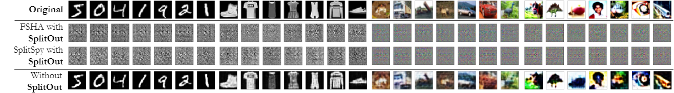
Figure 3: Results obtained by attackers for the MNIST, F-MNIST, CIFAR10, and CIFAR100 datasets with respect to the detection times (as shown in Table I). The first row displays the original images, and the last row displays the results obtained by a FSHA [36] attacker able to run for an arbitrary duration without being detected.

This seemingly contradicts the goal of collaborative ML, which was to outsource computation. However, as we will demonstrate in more detail, clients using a very small share of their local data for the data collection phase still perform accurate detection. Moreover, better data utilization, rather than purely outsourcing computation, might be a stronger reason for using SplitNN in certain scenarios (e.g. financially/technologically capable institutions such as universities or hospitals working on regulated private data). Since to collect training data for LOF we need only one epoch of training with 1% of the whole data, this is still feasible for many scenarios where SplitNN is employed. Recall that in SplitNN, the clients would train several layers (but not the whole neural network) with 100% of their data for multiple epochs, and increasing the number of client-side layers is recommended to make the private data more difficult to reconstruct from the intermediate outputs [14].

3.3 Detecting the Attack

When the SplitNN training begins, the gradients the server sends are input to LOF, and are classified as honest (inlier) or malicious (outlier). Clients can make a decision after each gradient or combine the results from multiple gradients, by classifying the last few gradients and reaching the final decision by a majority vote between them. If a client concludes that the server is launching an attack, it can stop training and prevent further progress of the attack.

For the LOF algorithm, clients need to decide on a hyperparameter $k$, the number of neighbors to consider. We have followed the existing work on automatically choosing the value of $k$ [62], and observed that setting it equal to one less than the number of honest gradients collected (i.e. the highest feasible value) consistently achieves the best performance across all our datasets.

Algorithm 1 explains the attack detection process in detail. Before training, clients allocate a certain share of their training data as a separate set $train_{\text{SIM}}$ and train the client-side layers together with a local copy of the server-side layers using that dataset (lines 10-13). The resulting gradients obtained from server-side layers then constitute the training data for outlier detection, denoted $train_{\text{LOF}}$ (line 12). During the actual training with SplitNN, clients receive the gradients from the server as part of the SplitNN protocol (line 17); each gradient received from the server is input to LOF (line 18), and classified as an outlier/inlier (lines 23-25). With the window size $w$, clients decide that the server is attacking if at least $w$ LOF decisions has been collected and the majority of them are outliers (i.e. malicious gradients). Simple bookkeeping is done to remove the earlier gradients so that the prediction set remains at size $w$ (line 19), and no decision is made for the first $w-1$ iterations (lines 20-22). Training is stopped as soon as an attack is detected.

It is possible to employ another outlier detection method in SplitOut besides LOF. We also experimented with other method such as one-class SVM [45] but found results employing LOF to be far superior, and hence present SplitOut and results as using LOF.

4 Evaluation & Discussion

4.1 Setup

For our experiments, we use the ResNet architecture [21], trained using Adam optimizer [27] with learning rate of 0.001, on the MNIST [32], Fashion-MNIST [60], and CIFAR10/100 [30] datasets. With a batch size of 64, one epoch is equal to 938 batches for MNIST and F-MNIST, and 782 batches for CIFAR10/100. We implemented SplitOut in Python (v 3.10) using the PyTorch (v 2.1.0) [37] and scikit-learn (v 1.2) [39] libraries.

We test SplitOut’s performance when trained on with different shares of client training data (1%, 10%, 25%, 50%, 75%, 100%) and different decision-window sizes (1, 10). As stated earlier, we set the number of neighbors to the highest possible value (i.e. one less than the number of training points): 937 for MNIST/F-MNIST, and 781 for CIFAR10/100 when whole training data was used. If the batch size is expressed as $N_{B}$, the selected number of neighbors $k$ can be calculated as $(\lfloor N_{B}\rfloor-1)$.

For each configuration, we measure the true and false positive rates by testing the method on 100 randomly-initialized runs each for the honest training scenario including training LOF from scratch, and each attack. A positive (attack detected) decision in a training-hijacking run is a true positive, and in an honest run is a false positive. To make sure we can detect the attack early enough, we start the algorithm after the required number of gradients for the decision window has been obtained.

TABLE II: SSIM [57] values comparing reconstructed images by the attackers with the original private image averaged over 10 runs. The bottom row displays SSIM results from FSHA’s reconstructed images without detection. A more successful reconstruction process is implied by a higher SSIM value.

	MNIST	F-MNIST	CIFAR	CIFAR100
FSHA with SplitOut	0.0004	0.0008	0.0002	0.0002
SplitSpy with SplitOut	0.0002	0.0004	0.0013	0.0001
Without detection	0.8902	0.6640	0.5035	0.2078

Figure 4: Results the FSHA attacker obtains when it performs multitask learning until detection for the MNIST, F-MNIST, CIFAR10, and CIFAR100 datasets, returning the gradients resulting from the average of honest training and adversarial objectives. The bottom row displays the original inputs.

4.2 Detecting Training-Hijacking

The effectiveness of SplitOut against all split learning training-hijacking attacks proposed so far (FSHA [36], backdoor attack [65], SplitSpy [16]) is displayed in Table I. We take the window size to be 10 and use as training data for LOF only $1\%$ of the clients’ data, which corresponds to e.g. 9 and 7 training iterations in F-/MNIST and CIFAR10/100 datasets, respectively, with a batch size of 64. More comprehensive results covering a wider range of hyperparameters can be found in Appendix A.

In the more simpler MNIST and F-MNIST datasets, SplitOut achieves a true positive rate (TPR) of 1 and a false positive rate (FPR) of 0, meaning it can detect whether there is an attack or not with perfect accuracy. For the more complex CIFAR datasets, $2\%$ of honest runs are classified as malicious, but that also reduces to zero as more data is allocated for LOF training (see Appendix A), resulting in a higher compute load for the clients. Importantly, LOF’s time to detect attacks does not vary significantly among the different training-hijacking attacks presented so far.

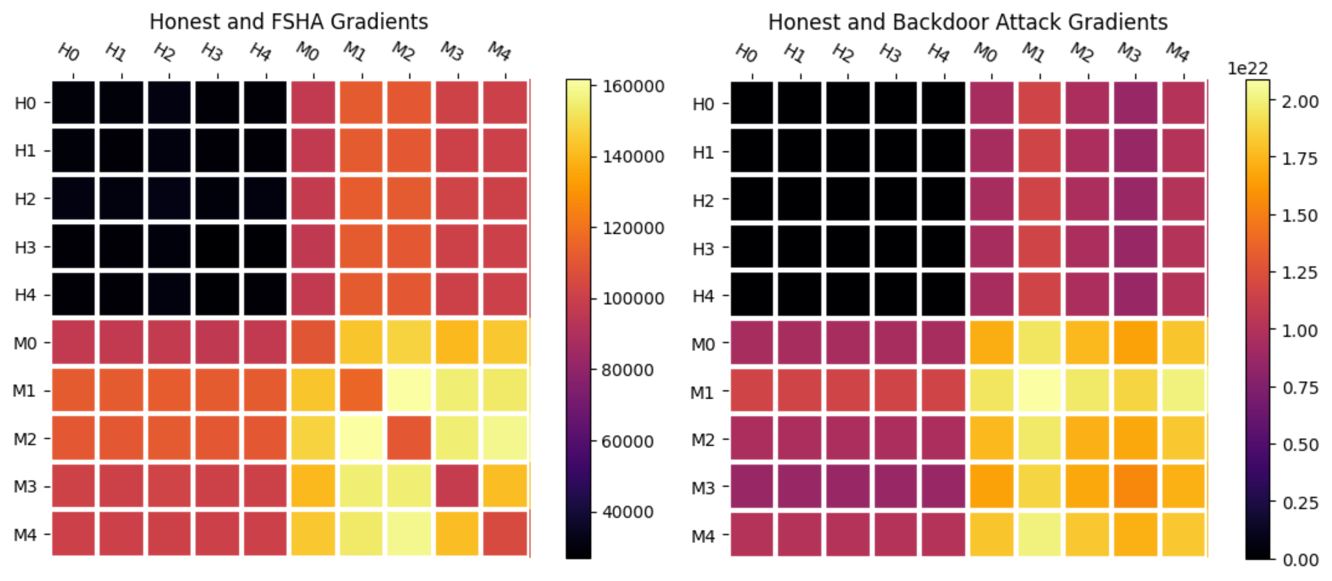
Figure 5: Pair-wise average $L_{2}$ distances between five randomly-chosen sets of gradients (corresponding to the first epoch of training) for honest training, FSHA [36] and the backdoor attack [65], each using the CIFAR10 dataset. In each of the plots, $H$ indicates honest gradients and $M$ malicious. Darker colors imply smaller values.

The structural similarity index measure (SSIM) [57] is a metric used to compare the quality of two different images. In our study, we used SSIM to estimate the image quality of the image reconstructed by the attacker, taking the original input image as a reference. For each dataset, SSIM values of 10 reconstructed images were calculated using the original image as reference, and their averages are shown in Table II. As previously shown in Figure 3 and indicated by the low SSIM values in Table II, SplitOut detects different attacks very early, preventing the malicious server from performing successful image reconstruction.

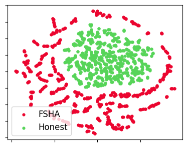
(a) FSHA

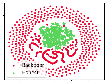
(b) Backdoor Attack

Figure 6: T-SNE [47] dimension reduction comparing honest and malicious (FSHA & the backdoor attack) gradients obtained from a randomly chosen run of the first epoch of training on CIFAR10.

4.3 Adaptive Attacks

To try to overcome a detection mechanism, a training-hijacking attacker can perform multitask learning and combine the feature-space alignment and honest training losses, e.g. by taking their average, and returning the resulting gradients to the client model. To demonstrate this scenario, we consider a FSHA attacker returning the average of the two losses. Table I displays our results against a multitasking FSHA (denoted FSHA-MT) attacker as well across our four benchmark datasets. We can detect all instances of the attack for on MNIST and CIFAR100 datasets, and 98% of the attack instances on F-MNIST and CIFAR10. Furthermore, Figure 4 displays the reconstruction results the attacker achieves under this setting. Compared to the results in Figure 3, the attack is expectedly less effective, since the client model is now updated to optimize the honest training loss as well as the adversarial discriminator loss.

To show that SplitOut can be used cooperatively with the earlier detection work, we also consider the scenario demonstrated in [16], where the training-hijacking attacker has full knowledge of the detection mechanism in [13]. We use our approach in tandem with the method of [13], and consider only the non-randomized batches as inputs to LOF. We use the name SplitSpy for this approach following [16] with the detection results displayed in Table I, where the LOF algorithm detects all instances of the attack similar to the earlier scenarios. This demonstrates that different detection methods can be used together and that even if the attacker circumvents the detection method of [13], the attack can still be detected using SplitOut.

4.4 Avoiding the Curse of Dimensionality

Our method of choice, the local outlier factor technique, is a distance-based method that makes frequent use of nearest-neighbor computations. Since the data we are working with is very high dimensional (e.g. 1728 dimensions for the gradients from the CIFAR tasks), the curse of dimensionality could have an adverse impact and lead to poor performance. More formally, it has been shown in [4] that for all $L_{p}$ norms with $p\geq 1$, as the dimensionality increases, the proportion $D_{\text{max}}/D_{\text{min}}$ of the distance $D_{\text{max}}$ to the farthest point and $D_{\text{min}}$ to the nearest point vanishes, meaning that the concept of a neighborhood basically collapses. Although $L_{p}$ norms with small $p$ values have been shown to be preferable in higher dimensions [1], they are still subject to the curse of dimensionality [67].

Thus, we now analyze the vast amount of data we collected throughout this work to explain the reasons behind the strong performance in a such high-dimensional setting. Figure 5 displays the pair-wise average $L_{2}$ distances between five randomly-chosen sets of gradients from honest training, as well as FSHA [36] and the backdoor attack [65] all corresponding to the first epoch of training. The results are highly informative about the global and local structure of the problem:

• Honest gradients are closer to honest gradients, as the top left quadrant is darker than the top right (and its symmetric bottom left) quadrant.

• Honest gradients are also closer to each other among themselves than malicious gradients are since the top left quadrant is darker than the bottom right quadrant.

• Malicious gradients are closer to honest gradients than they are to other malicious gradients since the bottom left (and top right) quadrants are darker than the bottom right quadrant.

These three observations together imply that the neighborhoods of honest gradients are more likely to be densely populated with honest gradients, while malicious gradients have sparser neighborhoods that contain a number of honest gradients as well as malicious ones.

The t-SNE [47] plots (Figure 6) displaying a dimension reduction of honest and malicious gradients over one epoch are consistent with the observations above since they also visualize honest gradients packed tightly, and malicious gradients covering a larger space essentially encompassing the honest gradients. This significant difference between honest and malicious neighborhoods is the main factor why a neighborhood-based method such as LOF succeeds in this task.

So we conclude that while neighborhood-based methods generally struggle in high dimensions, the intrinsic differences between the honest training and feature-space alignment optimization processes result in them having significantly different forms to their gradient updates, which gives rise to neighborhoods structures easily distinguishable through the $L_{2}$ distance despite the high dimensionality.

4.5 Computational Cost

As stated earlier, the core assumption behind SplitOut is that the clients can reasonably perform forward/backward passes over the entire model for a very small number of batches (e.g. 9 in case of F-/MNIST and 7 in CIFAR10/100). It has also been demonstrated as part of the earlier data reconstruction attacks [14, 36] that higher number of client-side layers makes client outputs harder to invert, giving rise to the privacy/cost trade-off inherent in many privacy-preserving systems. Thus, unlike earlier work on detecting training-hijacking attacks [13, 16] that relied on heuristical rather than computational assumptions as outlined in Section 2.4, our work extends this privacy/cost trade-off by instead giving up on task-related assumptions. This leads in turn to a simpler-to-use detection method that can be applied out-of-the-box without any hyperparameter tuning.

5 Related Work

Split learning has been shown to be vulnerable to various kinds of attacks beyond the training-hijacking literature we have covered. Regarding data privacy, split learning is vulnerable to model inversion attacks [14, 17, 41] aiming to reconstruct private client data, and label leakage attacks [14, 34, 33, 25], where the attacker (server) attempts to infer the private labels from the gradients sent by the client. Furthermore, confidentiality of the client models can be violated through model stealing attacks [14, 17], and the integrity of the system can be damaged through backdoor attacks [3].

Existence of such attacks has motivated the search for defense mechanisms. Differential privacy [12] has been applied to make private data reconstruction [18, 59] and label leakage [63] harder. Further work has considered integrating an additional optimization step to minimize the information the intermediate outputs leak [54], utilizing the permutation-equivariance of certain deep neural network components by shuffling the inputs without a cost to the model performance [61, 64], and using homomorphic encryption to compute part of the system on encrypted data to obtain formal guarantees on information leakage [26, 40].

6 Conclusion and Future Work

We demonstrated that SplitOut, an out-of-the-box outlier detection approach using the local outlier factor algorithm, can detect whether a split learning server is launching a training-hijacking attack or not with almost-perfect accuracy. Compared to earlier such detection work, we make stronger assumptions on the clients’ compute capabilities, but require fewer hyperparameters to be tuned, leading to a simpler to method that can be implemented readily using popular frameworks such as scikit-learn [39] on top of an existing split learning system. Due to the proactive design of our solution (performing outlier detection against honestly trained gradients), it can potentially detect some not-yet-known attacks.

Yet, a main limitation of SplitOut is that the space of training-hijacking attacks so far has been limited to feature-space alignment attacks. While such attacks have demonstrated strong performance for data reconstruction and implementing backdoors, future attacks employing a different training-hijacking approach could potentially behave in a different way than the observations we made in Section 4.4 and make our approach less effective. We leave this as future work.

Appendix A Comprehensive Results For Attack Detection

In this section, we provide our ablation study results. Clients collect training data for LOF by training the entire model over one epoch, with some portion of their data. During this training process, the impact of using their data at different fractions on attack detection was examined. SplitOut’s performance against FSHA [36], backdoor [65] and SplitSpy [16] is shown respectively in Tables I(a), II(a) and III(a), when trained with different shares of client training data (1%, 10%, 25%, 50%, 75%, 100%) and different decision-window sizes (1, 10).

TABLE I: Detecting FSHA using SplitOut [36]. True and false positive rates for our method averaged over 100 runs. LOF data rate is the percentage of client data used in simulating the entire model to obtain training data for the LOF algorithm. Window size is the number of most recent single-gradient decisions to perform a majority vote over to reach the final decision. The $t$ field denotes the average point of detection (as the share of total number of batches).

(a) Window size: 1

Dataset $\rightarrow$	MNIST			F-MNIST			CIFAR10			CIFAR100
LOF Data Rate (%) $\downarrow$	TPR	FPR	$t$	TPR	FPR	$t$	TPR	FPR	$t$	TPR	FPR	$t$
1	1.0	0.03	0.0013	1.0	0.02	0.0023	1.0	0.58	0.0043	1.0	0.70	0.0590
10	1.0	0.03	0.0013	1.0	0.01	0.0023	1.0	0.07	0.0076	1.0	0.23	0.0111
25	1.0	0.03	0.0013	1.0	0.01	0.0023	1.0	0.01	0.0089	1.0	0.10	0.0129
50	1.0	0.03	0.0013	1.0	0.01	0.0023	1.0	0.01	0.0097	1.0	0.02	0.0195
75	1.0	0.03	0.0013	1.0	0.01	0.0024	1.0	0.01	0.0108	1.0	0.03	0.0265
100	1.0	0.03	0.0013	1.0	0.00	0.0024	1.0	0.01	0.0117	1.0	0.02	0.0354

(b) Window size: 10

Dataset $\rightarrow$	MNIST			F-MNIST			CIFAR10			CIFAR100
LOF Data Rate (%) $\downarrow$	TPR	FPR	$t$	TPR	FPR	$t$	TPR	FPR	$t$	TPR	FPR	$t$
1	1.0	0.0	0.0107	1.0	0.0	0.0109	1.0	0.02	0.0132	1.0	0.02	0.0142
10	1.0	0.0	0.0107	1.0	0.0	0.0109	1.0	0.00	0.0145	1.0	0.00	0.0219
25	1.0	0.0	0.0107	1.0	0.0	0.0109	1.0	0.00	0.0156	1.0	0.00	0.0289
50	1.0	0.0	0.0107	1.0	0.0	0.0109	1.0	0.00	0.0170	1.0	0.00	0.0357
75	1.0	0.0	0.0107	1.0	0.0	0.0109	0.99	0.00	0.0170	1.0	0.00	0.0434
100	1.0	0.0	0.0107	1.0	0.0	0.0109	0.99	0.00	0.0183	1.0	0.00	0.0557

TABLE II: Detecting the Backdoor Attack using SplitOut [65]. True and false positive rates for our method averaged over 100 runs. LOF data rate is the percentage of client data used in simulating the entire model to obtain training data for the LOF algorithm. Window size is the number of most recent single-gradient decisions to perform a majority vote over to reach the final decision. The $t$ field denotes the average point of detection (as the share of total number of batches).

(a) Window size: 1

Dataset $\rightarrow$	MNIST			F-MNIST			CIFAR10			CIFAR100
LOF Data Rate (%) $\downarrow$	TPR	FPR	$t$	TPR	FPR	$t$	TPR	FPR	$t$	TPR	FPR	$t$
1	1.0	0.03	0.0011	1.0	0.02	0.0011	1.0	0.58	0.0026	1.0	0.70	0.0028
10	1.0	0.03	0.0011	1.0	0.01	0.0011	1.0	0.07	0.0036	1.0	0.23	0.0039
25	1.0	0.03	0.0011	1.0	0.01	0.0011	1.0	0.01	0.0038	1.0	0.10	0.0041
50	1.0	0.03	0.0011	1.0	0.01	0.0011	1.0	0.01	0.0039	1.0	0.02	0.0044
75	1.0	0.03	0.0011	1.0	0.01	0.0011	1.0	0.01	0.0039	1.0	0.03	0.0045
100	1.0	0.03	0.0011	1.0	0.00	0.0011	1.0	0.01	0.0040	1.0	0.02	0.0046

(b) Window size: 10

Dataset $\rightarrow$	MNIST			F-MNIST			CIFAR10			CIFAR100
LOF Data Rate (%) $\downarrow$	TPR	FPR	$t$	TPR	FPR	$t$	TPR	FPR	$t$	TPR	FPR	$t$
1	1.0	0.0	0.0106	1.0	0.0	0.0107	1.0	0.02	0.0128	1.0	0.02	0.0128
10	1.0	0.0	0.0106	1.0	0.0	0.0107	1.0	0.00	0.0128	1.0	0.00	0.0128
25	1.0	0.0	0.0106	1.0	0.0	0.0107	1.0	0.00	0.0128	1.0	0.00	0.0128
50	1.0	0.0	0.0106	1.0	0.0	0.0107	1.0	0.00	0.0128	1.0	0.00	0.0128
75	1.0	0.0	0.0107	1.0	0.0	0.0107	1.0	0.00	0.0128	1.0	0.00	0.0128
100	1.0	0.0	0.0107	1.0	0.0	0.0107	1.0	0.00	0.0128	1.0	0.00	0.0128

TABLE III: Detecting SplitSpy using SplitOut [16]. True and false positive rates for our method averaged over 100 runs. LOF data rate is the percentage of client data used in simulating the entire model to obtain training data for the LOF algorithm. Window size is the number of most recent single-gradient decisions to perform a majority vote over to reach the final decision. The $t$ field denotes the average point of detection (as the share of total number of batches).

(a) Window size: 1

Dataset $\rightarrow$	MNIST			F-MNIST			CIFAR10			CIFAR100
LOF Data Rate (%) $\downarrow$	TPR	FPR	$t$	TPR	FPR	$t$	TPR	FPR	$t$	TPR	FPR	$t$
1	1.0	0.03	0.001	1.0	0.02	0.0011	1.0	0.58	0.0052	1.0	0.70	0.0056
10	1.0	0.03	0.001	1.0	0.01	0.0011	1.0	0.07	0.0082	1.0	0.23	0.0101
25	1.0	0.03	0.001	1.0	0.01	0.0011	1.0	0.01	0.0100	1.0	0.10	0.1230
50	1.0	0.03	0.001	1.0	0.01	0.0011	1.0	0.01	0.0106	1.0	0.02	0.0171
75	1.0	0.03	0.001	1.0	0.01	0.0012	1.0	0.01	0.0102	1.0	0.03	0.0208
100	1.0	0.03	0.001	1.0	0.00	0.0012	1.0	0.01	0.0114	1.0	0.02	0.0227

(b) Window size: 10

Dataset $\rightarrow$	MNIST			F-MNIST			CIFAR10			CIFAR100
LOF Data Rate (%) $\downarrow$	TPR	FPR	$t$	TPR	FPR	$t$	TPR	FPR	$t$	TPR	FPR	$t$
1	1.0	0.0	0.0106	1.0	0.0	0.0107	1.00	0.02	0.0137	1.0	0.02	0.0173
10	1.0	0.0	0.0106	1.0	0.0	0.0107	1.00	0.00	0.0100	1.0	0.00	0.0199
25	1.0	0.0	0.0106	1.0	0.0	0.0107	0.99	0.00	0.0158	1.0	0.00	0.0250
50	1.0	0.0	0.0106	1.0	0.0	0.0107	0.99	0.00	0.0164	1.0	0.00	0.0347
75	1.0	0.0	0.0106	1.0	0.0	0.0107	1.00	0.00	0.0169	1.0	0.00	0.0423
100	1.0	0.0	0.0106	1.0	0.0	0.0107	0.99	0.00	0.0174	1.0	0.00	0.0456

References

- Aggarwal et al., [2001] Aggarwal, C. C., Hinneburg, A., and Keim, D. A. (2001). On the Surprising Behavior of Distance Metrics in High Dimensional Space. In Goos, G., Hartmanis, J., Van Leeuwen, J., Van Den Bussche, J., and Vianu, V., editors, Database Theory — ICDT 2001, volume 1973, pages 420–434. Springer Berlin Heidelberg, Berlin, Heidelberg.
- Annas, [2003] Annas, G. J. (2003). HIPAA Regulations — A New Era of Medical-Record Privacy? New England Journal of Medicine, 348(15):1486–1490.
- Bai et al., [2023] Bai, Y., Chen, Y., Zhang, H., Xu, W., Weng, H., and Goodman, D. (2023). VILLAIN: Backdoor attacks against vertical split learning. In 32nd USENIX Security Symposium (USENIX Security 23), pages 2743–2760.
- Beyer et al., [1999] Beyer, K., Goldstein, J., Ramakrishnan, R., and Shaft, U. (1999). When is “nearest neighbor” meaningful? In Database Theory—ICDT’99: 7th International Conference Jerusalem, Israel, January 10–12, 1999 Proceedings 7, pages 217–235. Springer.
- Bonawitz et al., [2019] Bonawitz, K., Eichner, H., Grieskamp, W., Huba, D., Ingerman, A., Ivanov, V., Kiddon, C., Konečnỳ, J., Mazzocchi, S., McMahan, B., et al. (2019). Towards federated learning at scale: System design. Proceedings of Machine Learning and Systems, 1:374–388.
- Breunig et al., [2000] Breunig, M. M., Kriegel, H.-P., Ng, R. T., and Sander, J. (2000). Lof: identifying density-based local outliers. In ACM SIGMOD, pages 93–104.
- Bronstein et al., [2021] Bronstein, M. M., Bruna, J., Cohen, T., and Veličković, P. (2021). Geometric deep learning: Grids, groups, graphs, geodesics, and gauges. arXiv preprint arXiv:2104.13478.
- Brown et al., [2020] Brown, T. B., Mann, B., Ryder, N., Subbiah, M., Kaplan, J., Dhariwal, P., Neelakantan, A., Shyam, P., Sastry, G., Askell, A., Agarwal, S., Herbert-Voss, A., Krueger, G., Henighan, T., Child, R., Ramesh, A., Ziegler, D. M., Wu, J., Winter, C., Hesse, C., Chen, M., Sigler, E., Litwin, M., Gray, S., Chess, B., Clark, J., Berner, C., McCandlish, S., Radford, A., Sutskever, I., and Amodei, D. (2020). Language Models are Few-Shot Learners. arXiv:2005.14165 [cs]. arXiv: 2005.14165.
- Carlini et al., [2023] Carlini, N., Hayes, J., Nasr, M., Jagielski, M., Sehwag, V., Tramer, F., Balle, B., Ippolito, D., and Wallace, E. (2023). Extracting training data from diffusion models. In 32nd USENIX Security Symposium (USENIX Security 23), pages 5253–5270.
- Chen et al., [2010] Chen, S., Wang, W., and van Zuylen, H. (2010). A comparison of outlier detection algorithms for its data. Expert Systems with Applications, 37(2):1169–1178.
- Devlin et al., [2018] Devlin, J., Chang, M.-W., Lee, K., and Toutanova, K. (2018). Bert: Pre-training of deep bidirectional transformers for language understanding. arXiv preprint arXiv:1810.04805.
- Dwork et al., [2014] Dwork, C., Roth, A., et al. (2014). The algorithmic foundations of differential privacy. Found. Trends Theor. Comput. Sci., 9(3-4):211–407.
- Erdogan et al., [2022] Erdogan, E., Küpçü, A., and Cicek, A. E. (2022). Splitguard: Detecting and mitigating training-hijacking attacks in split learning. In ACM WPES, page 125–137.
- Erdoğan et al., [2022] Erdoğan, E., Küpçü, A., and Çiçek, A. E. (2022). Unsplit: Data-oblivious model inversion, model stealing, and label inference attacks against split learning. In ACM WPES, page 115–124.
- Fredrikson et al., [2015] Fredrikson, M., Jha, S., and Ristenpart, T. (2015). Model inversion attacks that exploit confidence information and basic countermeasures. In Proceedings of the 22nd ACM SIGSAC conference on computer and communications security, pages 1322–1333.
- Fu et al., [2023] Fu, J., Ma, X., Zhu, B., Hu, P., Zhao, R., Jia, Y., Xu, P., Jin, H., and Zhang, D. (2023). Focusing on Pinocchio’s Nose: A Gradients Scrutinizer to Thwart Split-Learning Hijacking Attacks Using Intrinsic Attributes.
- Gao and Zhang, [2023] Gao, X. and Zhang, L. (2023). PCAT: Functionality and data stealing from split learning by Pseudo-Client attack. In 32nd USENIX Security Symposium (USENIX Security 23), pages 5271–5288.
- Gawron and Stubbings, [2022] Gawron, G. and Stubbings, P. (2022). Feature space hijacking attacks against differentially private split learning. Third AAAI Workshop on Privacy-Preserving Artificial Intelligence.
- Goodfellow et al., [2016] Goodfellow, I., Bengio, Y., and Courville, A. (2016). Deep Learning. MIT Press. http://www.deeplearningbook.org.
- Gupta and Raskar, [2018] Gupta, O. and Raskar, R. (2018). Distributed learning of deep neural network over multiple agents. Journal of Network and Computer Applications, 116:1–8.
- He et al., [2016] He, K., Zhang, X., Ren, S., and Sun, J. (2016). Deep residual learning for image recognition. In Proceedings of the IEEE conference on computer vision and pattern recognition, pages 770–778.
- Hendrycks et al., [2021] Hendrycks, D., Carlini, N., Schulman, J., and Steinhardt, J. (2021). Unsolved problems in ml safety. arXiv preprint arXiv:2109.13916.
- Hornik, [1991] Hornik, K. (1991). Approximation capabilities of multilayer feedforward networks. Neural networks, 4(2):251–257.
- Janssens et al., [2009] Janssens, J. H., Flesch, I., and Postma, E. O. (2009). Outlier detection with one-class classifiers from ml and kdd. In 2009 International Conference on Machine Learning and Applications, pages 147–153. IEEE.
- Kariyappa and Qureshi, [2023] Kariyappa, S. and Qureshi, M. K. (2023). Exploit: Extracting private labels in split learning. In 2023 IEEE Conference on Secure and Trustworthy Machine Learning (SaTML), pages 165–175.
- Khan et al., [2023] Khan, T., Nguyen, K., Michalas, A., and Bakas, A. (2023). Love or hate? share or split? privacy-preserving training using split learning and homomorphic encryption. arXiv preprint arXiv:2309.10517.
- Kingma and Ba, [2017] Kingma, D. P. and Ba, J. (2017). Adam: A Method for Stochastic Optimization. arXiv:1412.6980 [cs]. arXiv: 1412.6980.
- Kipf and Welling, [2016] Kipf, T. N. and Welling, M. (2016). Semi-supervised classification with graph convolutional networks. arXiv preprint arXiv:1609.02907.
- Konečný et al., [2016] Konečný, J., McMahan, H. B., Ramage, D., and Richtárik, P. (2016). Federated Optimization: Distributed Machine Learning for On-Device Intelligence. arXiv:1610.02527 [cs]. arXiv: 1610.02527.
- Krizhevsky, [2009] Krizhevsky, A. (2009). Learning multiple layers of features from tiny images. Master’s thesis, University of Toronto.
- LeCun et al., [1995] LeCun, Y., Bengio, Y., et al. (1995). Convolutional networks for images, speech, and time series. The handbook of brain theory and neural networks, 3361(10):1995.
- LeCun et al., [2010] LeCun, Y., Cortes, C., and Burges, C. (2010). Mnist handwritten digit database. ATT Labs [Online]. Available: http://yann.lecun.com/exdb/mnist, 2.
- Li et al., [2021] Li, O., Sun, J., Yang, X., Gao, W., Zhang, H., Xie, J., Smith, V., and Wang, C. (2021). Label leakage and protection in two-party split learning. arXiv preprint arXiv:2102.08504.
- Liu and Lyu, [2022] Liu, J. and Lyu, X. (2022). Clustering label inference attack against practical split learning. arXiv preprint arXiv:2203.05222.
- Mercuri, [2004] Mercuri, R. T. (2004). The HIPAA-potamus in health care data security. Communications of the ACM, 47(7):25–28.
- Pasquini et al., [2021] Pasquini, D., Ateniese, G., and Bernaschi, M. (2021). Unleashing the tiger: Inference attacks on split learning. In ACM CCS, pages 2113–2129.
- Paszke et al., [2019] Paszke, A., Gross, S., Massa, F., Lerer, A., Bradbury, J., Chanan, G., Killeen, T., Lin, Z., Gimelshein, N., Antiga, L., Desmaison, A., Kopf, A., Yang, E., DeVito, Z., Raison, M., Tejani, A., Chilamkurthy, S., Steiner, B., Fang, L., Bai, J., and Chintala, S. (2019). Pytorch: An imperative style, high-performance deep learning library. In NeurIPS, pages 8024–8035.
- Patterson et al., [2021] Patterson, D., Gonzalez, J., Le, Q., Liang, C., Munguia, L.-M., Rothchild, D., So, D., Texier, M., and Dean, J. (2021). Carbon emissions and large neural network training. arXiv preprint arXiv:2104.10350.
- Pedregosa et al., [2011] Pedregosa, F., Varoquaux, G., Gramfort, A., Michel, V., Thirion, B., Grisel, O., Blondel, M., Prettenhofer, P., Weiss, R., Dubourg, V., Vanderplas, J., Passos, A., Cournapeau, D., Brucher, M., Perrot, M., and Duchesnay, E. (2011). Scikit-learn: Machine learning in Python. Journal of Machine Learning Research, 12:2825–2830.
- Pereteanu et al., [2022] Pereteanu, G.-L., Alansary, A., and Passerat-Palmbach, J. (2022). Split he: Fast secure inference combining split learning and homomorphic encryption. arXiv preprint arXiv:2202.13351.
- Qiu et al., [2023] Qiu, X., Leontiadis, I., Melis, L., Sablayrolles, A., and Stock, P. (2023). EXACT: Extensive Attack for Split Learning.
- Rombach et al., [2022] Rombach, R., Blattmann, A., Lorenz, D., Esser, P., and Ommer, B. (2022). High-resolution image synthesis with latent diffusion models. In Proceedings of the IEEE/CVF conference on computer vision and pattern recognition, pages 10684–10695.
- Rosenblatt, [1958] Rosenblatt, F. (1958). The perceptron: a probabilistic model for information storage and organization in the brain. Psychological review, 65(6):386.
- Rumelhart et al., [1986] Rumelhart, D. E., Hinton, G. E., and Williams, R. J. (1986). Learning representations by back-propagating errors. nature, 323(6088):533–536.
- Schölkopf et al., [1999] Schölkopf, B., Williamson, R. C., Smola, A., Shawe-Taylor, J., and Platt, J. (1999). Support vector method for novelty detection. Advances in neural information processing systems, 12.
- Singh et al., [2019] Singh, A., Vepakomma, P., Gupta, O., and Raskar, R. (2019). Detailed comparison of communication efficiency of split learning and federated learning. arXiv preprint arXiv:1909.09145.
- Van der Maaten and Hinton, [2008] Van der Maaten, L. and Hinton, G. (2008). Visualizing data using t-sne. Journal of machine learning research, 9(11).
- Vapnik, [1991] Vapnik, V. (1991). Principles of risk minimization for learning theory. Advances in neural information processing systems, 4.
- Vaswani et al., [2017] Vaswani, A., Shazeer, N., Parmar, N., Uszkoreit, J., Jones, L., Gomez, A. N., Kaiser, Ł., and Polosukhin, I. (2017). Attention is all you need. Advances in neural information processing systems, 30.
- Veale et al., [2018] Veale, M., Binns, R., and Edwards, L. (2018). Algorithms that Remember: Model Inversion Attacks and Data Protection Law. Philosophical Transactions of the Royal Society A: Mathematical, Physical and Engineering Sciences, 376(2133):20180083.
- Veale and Zuiderveen Borgesius, [2021] Veale, M. and Zuiderveen Borgesius, F. (2021). Demystifying the draft eu artificial intelligence act—analysing the good, the bad, and the unclear elements of the proposed approach. Computer Law Review International, 22(4):97–112.
- Veličković, [2023] Veličković, P. (2023). Everything is connected: Graph neural networks. Current Opinion in Structural Biology, 79:102538.
- [53] Vepakomma, P., Gupta, O., Swedish, T., and Raskar, R. (2018a). Split learning for health: Distributed deep learning without sharing raw patient data. arXiv preprint arXiv:1812.00564.
- Vepakomma et al., [2020] Vepakomma, P., Singh, A., Gupta, O., and Raskar, R. (2020). NoPeek: Information leakage reduction to share activations in distributed deep learning. In 2020 International Conference on Data Mining Workshops (ICDMW), pages 933–942, Sorrento, Italy. IEEE.
- [55] Vepakomma, P., Swedish, T., Raskar, R., Gupta, O., and Dubey, A. (2018b). No peek: A survey of private distributed deep learning. arXiv preprint arXiv:1812.03288.
- Wang et al., [2019] Wang, B., Yao, Y., Shan, S., Li, H., Viswanath, B., Zheng, H., and Zhao, B. Y. (2019). Neural cleanse: Identifying and mitigating backdoor attacks in neural networks. In 2019 IEEE Symposium on Security and Privacy (SP), pages 707–723. IEEE.
- Wang et al., [2004] Wang, Z., Bovik, A., Sheikh, H., and Simoncelli, E. (2004). Image Quality Assessment: From Error Visibility to Structural Similarity. IEEE Transactions on Image Processing, 13(4):600–612.
- White House Office of Science and Technology Policy, [2023] White House Office of Science and Technology Policy (2023). Blueprint for an ai bill of rights.
- Wu et al., [2023] Wu, M., Cheng, G., Li, P., Yu, R., Wu, Y., Pan, M., and Lu, R. (2023). Split learning with differential privacy for integrated terrestrial and non-terrestrial networks. IEEE Wireless Communications.
- Xiao et al., [2017] Xiao, H., Rasul, K., and Vollgraf, R. (2017). Fashion-mnist: a novel image dataset for benchmarking machine learning algorithms. arXiv preprint arXiv:1708.07747.
- Xu et al., [2023] Xu, H., Xiang, L., Ye, H., Yao, D., Chu, P., and Li, B. (2023). Shuffled Transformer for Privacy-Preserving Split Learning.
- Xu et al., [2019] Xu, Z., Kakde, D., and Chaudhuri, A. (2019). Automatic hyperparameter tuning method for local outlier factor, with applications to anomaly detection. In 2019 IEEE International Conference on Big Data (Big Data), pages 4201–4207. IEEE.
- Yang et al., [2022] Yang, X., Sun, J., Yao, Y., Xie, J., and Wang, C. (2022). Differentially private label protection in split learning. arXiv preprint arXiv:2203.02073.
- Yao et al., [2022] Yao, D., Xiang, L., Xu, H., Ye, H., and Chen, Y. (2022). Privacy-Preserving Split Learning via Patch Shuffling over Transformers. In 2022 IEEE International Conference on Data Mining (ICDM), pages 638–647.
- Yu et al., [2023] Yu, F., Wang, L., Zeng, B., Zhao, K., Pang, Z., and Wu, T. (2023). How to backdoor split learning. Neural Networks, 168:326–336.
- Zhu et al., [2019] Zhu, L., Liu, Z., and Han, S. (2019). Deep leakage from gradients. Advances in neural information processing systems, 32.
- Zimek et al., [2012] Zimek, A., Schubert, E., and Kriegel, H.-P. (2012). A survey on unsupervised outlier detection in high-dimensional numerical data. Statistical Analysis and Data Mining: The ASA Data Science Journal, 5(5):363–387.