Uncertainty-Aware Instance Reweighting for Off-Policy Learning

Abstract

Off-policy learning, referring to the procedure of policy optimization with access only to logged feedback data, has shown importance in various important real-world applications, such as search engines and recommender systems. While the ground-truth logging policy is usually unknown, previous work simply takes its estimated value for the off-policy learning, ignoring the negative impact from both high bias and high variance resulted from such an estimator. And these impact is often magnified on samples with small and inaccurately estimated logging probabilities. The contribution of this work is to explicitly model the uncertainty in the estimated logging policy, and propose an Uncertainty-aware Inverse Propensity Score estimator (UIPS) for improved off-policy learning, with a theoretical convergence guarantee. Experiment results on the synthetic and real-world recommendation datasets demonstrate that UIPS significantly improves the quality of the discovered policy, when compared against an extensive list of state-of-the-art baselines.

1 Introduction

In many real-world applications, including search engines Agarwal et al. (2019), online advertisements Strehl et al. (2010), recommender systems Chen et al. (2019); Liu et al. (2022), only logged data is available for subsequent policy learning. For example, in recommender systems, various complex recommendation policies are optimized over logged user interactions (e.g., clicks or stay time) with items recommended by previous recommendation policies (referred to as the logging policy) Zhou et al. (2018); Guo et al. (2017). However, such logged data is often known to be biased, since the feedback on items where the logging policy did not take is unknown. This inevitably distorts the evaluation and optimization of a new policy when it differs from the logging policy.

Off-policy learning Thrun and Littman (2000); Precup (2000) thus emerges as a preferred way to learn an improved policy only from the logged data, by addressing the mismatch between the learning and logging policies. One of the most commonly used off-policy learning methods is the Inverse Propensity Scoring (IPS) Chen et al. (2019); Munos et al. (2016), which assigns per-sample importance weight (i.e., propensity score) to the training objective on the logged data, so as to get an unbiased optimization objective in expectation. The importance weight in IPS is the probability ratio of taking an action between the learning and logging policies.

Unfortunately, oftentimes in practice the ground-truth logging policy is unavailable to the learner, e.g., it is not recorded in the data. One common treatment by many previous work Strehl et al. (2010); Liu et al. (2022); Chen et al. (2019); Ma et al. (2020) is to first estimate the logging policy using a supervised learning method (e.g., logistic regression, neural networks, etc.), and then take the estimated logging policy for off-policy learning. In this work, we first show that such an approximation results in a biased estimator which is sensitive to data with small estimated logging probabilities. Worse still, small estimated logging probabilities usually suggest there are limited related samples in the logged data, whose estimations can have high uncertainties, i.e., being wrong with a high probability. Figure 1 shows a piece of empirical evidence from a large-scale recommendation benchmark KuaiRec dataset Gao et al. (2022), where items with lower frequencies in the logged dataset have lower estimated logging probabilities (via a neural network estimator) and higher uncertainties at the same time. The high bias and variance caused by these samples can greatly hinder the performance of subsequent off-policy learning. We defer detailed discussions of this result in Section 2.

(a) Estimated Logging Probability

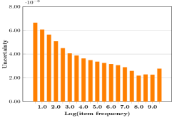
(b) Uncertainty of Estimation

Figure 1: Estimated logging policy and its uncertainty under different item frequency on KuaiRec.

In this work, we explicitly take the uncertainty of the estimated logging policy into consideration and design an Uncertainty-aware Inverse Propensity Score estimator (UIPS) for off-policy learning. UIPS reweighs the propensity score of each logged sample to control its impact on policy optimization, and learns an improved policy by alternating between: (1) Find the optimal weight that makes the estimator as accurate as possible, based on the uncertainty of the estimated logging policy; (2) Improve the policy by optimizing the resulting objective function. The optimal weight for each sample is obtained by minimizing the upper bound of the mean squared error (MSE) to the ground-truth policy evaluation, with a closed-form solution. Furthermore, UIPS ensures that off-policy learning converges to a stationary point where the true policy gradient is zero; while convergence may not be guaranteed when directly using the estimated logging policy. Extensive experiments on a synthetic and three real-world recommendation datasets against a rich set of state-of-the-art baselines demonstrate the power of UIPS. All data and code can be found in supplementary materials for reproducibility.

2 Preliminary: off-policy learning

We focus on the standard contextual bandit setup to explain the key concepts in UIPS. Following the convention Joachims et al. (2018); Saito and Joachims (2022); Su et al. (2020), let $\bm{x}\in\mathcal{X}\subseteq R^{d}$ be a $d$-dimensional context vector drawn from an unknown distribution $p(\bm{x})$. Each context is associated with a finite set of actions denoted by $\mathcal{A}$, where $|\mathcal{A}|<\infty$. Let $\pi:\mathcal{A}\times\mathcal{X}\rightarrow[0,1]$ denote a stochastic policy, such that $\pi(a|\bm{x})$ is the probability of selecting action $a$ under context $\bm{x}$ and $\sum_{a\in\mathcal{A}}\pi(a|\bm{x})=1$. Under a given context, the reward $r_{\bm{x},a}$ is only observed when action $a$ is chosen, i.e., bandit feedback. Without loss of generality, we assume $r_{\bm{x},a}\in[0,1]$. Let $V(\pi)$ denote the expected reward of the policy $\pi$:

$$V(\pi)=\mathbb{E}_{\bm{x}\sim p(\bm{x}),a\sim\pi(a|\bm{x})}[r_{\bm{x},a}].$$ (1)

We look for a policy $\pi(a|\bm{x})$ to maximize $V(\pi)$. In the rest, we denote $\mathbb{E}_{\bm{x}\sim p(\bm{x}),a\sim\pi(a|\bm{x})}[\cdot]$ as $\mathbb{E}_{\pi}[\cdot]$.

In off-policy learning, one can only access a set of logged feedback data $D:=\{(\bm{x}_{n},a_{n},r_{\bm{x}_{n},a_{n}})|n\in[N]\}$. Given $\bm{x}_{n}$, the action $a_{n}$ was generated by a stochastic logging policy $\beta^{\ast}$, i.e., $a_{n}\sim\beta^{\ast}(a|\bm{x}_{n})$, which is usually different from the learning policy $\pi(a|\bm{x})$ Ma et al. (2020); Swaminathan et al. (2017); Chen et al. (2019). The actions $\{a_{1},\ldots,a_{N}\}$ and their corresponding rewards $\{r_{\bm{x}_{1},a_{1}},\ldots,r_{\bm{x}_{N},a_{N}}\}$ are generated independently given $\beta^{\ast}$. The main challenge is then to address the distributional discrepancy between $\beta^{*}(a|\bm{x})$ and $\pi(a|\bm{x})$, when optimizing $\pi(a|\bm{x})$ to maximize $V(\pi)$ with access only to the logged dataset $D$.

One of the most widely used methods to address the distribution shift between $\pi(a|\bm{x})$ and $\beta^{*}(a|\bm{x})$ is the Inverse Propensity Scoring (IPS) Chen et al. (2019); Munos et al. (2016). One can easily get that:

$$V(\pi)=\mathbb{E}_{\beta^{*}}\left[\frac{\pi(a|\bm{x})}{\beta^{*}(a|\bm{x})}r_{\bm{x},a}\right],$$

yielding the following empirical estimator of $V(\pi)$:

$$\hat{V}_{{\rm IPS}}(\pi)=\frac{1}{N}\sum_{n=1}^{N}\frac{\pi(a_{n}|\bm{x}_{n})}{\beta^{*}(a_{n}|\bm{x}_{n})}r_{\bm{x}_{n},a_{n}},$$ (2)

where $\pi(a_{n}|\bm{x}_{n})/\beta^{*}(a_{n}|\bm{x}_{n})$ is referred to as the propensity score. Various algorithms can be readily used for policy optimization under $\hat{V}_{{\rm IPS}}(\pi)$, including value-based methods Silver et al. (2016) and policy-based methods Levine and Koltun (2013); Schulman et al. (2015); Williams (1992). In this work, we adopt a well-known policy gradient algorithm, REINFORCE Williams (1992). Assume the policy $\pi(a|\bm{x})$ is parameterized by $\bm{\vartheta}$, via the “log-trick”, the gradient of $\hat{V}_{{\rm IPS}}(\pi_{\bm{\vartheta}})$ with respect to $\bm{\vartheta}$ can be readily derived as,

$$\nabla_{\bm{\vartheta}}\hat{V}_{{\rm IPS}}(\pi_{\bm{\vartheta}})=\frac{1}{N}\sum_{n=1}^{N}\frac{\pi_{\bm{\vartheta}}(a_{n}|\bm{x}_{n})}{\beta^{*}(a_{n}|\bm{x}_{n})}r_{\bm{x}_{n},a_{n}}\nabla_{\bm{\vartheta}}\log(\pi_{\bm{\vartheta}}(a_{n}|\bm{x}_{n})).\vspace{-1mm}$$

Approximation with an unknown logging policy. In many real-world applications, the ground-truth logging probabilities, i.e., $\beta^{*}(a|\bm{x})$ of each observation $(\bm{x},a)$ in $D$, are unknown. One primary reason is the legacy issue, i.e., the probabilities were not logged when collecting data. As a typical walk-around, previous work employs supervised learning methods such as logistic regression Schnabel et al. (2016) and nerural networks Chen et al. (2019) to estimate the logging policy, and replaces $\beta^{*}(a|\bm{x})$ with its estimated value $\hat{\beta}(a|\bm{x})$ to get the following BIPS estimator for policy learning:

$$\hat{V}_{{\rm BIPS}}(\pi_{\bm{\vartheta}})=\frac{1}{N}\sum_{n=1}^{N}\frac{\pi_{\bm{\vartheta}}(a_{n}|\bm{x}_{n})}{\hat{\beta}(a_{n}|\bm{x}_{n})}r_{\bm{x}_{n},a_{n}}.\vspace{-0.5mm}$$ (3)

However, as shown in the following proposition, inaccurate $\hat{\beta}(a|\bm{x})$ leads to high bias and variance in BIPS. Worse still, smaller and inaccurate $\hat{\beta}(a|\bm{x})$ further enlarges this bias and variance.

Proposition 2.1

The bias and variance of $\hat{V}_{{\rm BIPS}}(\pi_{\bm{\vartheta}})$ can be derived as follows:

$${\rm Bias\left(\hat{V}_{{\rm BIPS}}(\pi_{\bm{\vartheta}})\right)}=\mathbb{E}_{D}\left[\hat{V}_{{\rm BIPS}}(\pi_{\bm{\vartheta}})-V(\pi_{\bm{\vartheta}})\right]=\mathbb{E}_{\pi_{\bm{\vartheta}}}\left[r_{\bm{x},a}\left(\frac{\beta^{*}(a|\bm{x})}{\hat{\beta}(a|\bm{x})}-1\right)\right]$$

$$N\cdot{\rm Var}_{D}\left(\hat{V}_{{\rm BIPS}}(\pi_{\bm{\vartheta}})\right)={\rm Var}_{\pi_{\bm{\vartheta}}}\left(\frac{\beta^{*}(a|\bm{x})}{\hat{\beta}(a|\bm{x})}r_{\bm{x},a}\right)+\mathbb{E}_{\pi_{\bm{\vartheta}}}\left[\left(\frac{\pi_{\bm{\vartheta}}(a|\bm{x})}{\beta^{*}(a|\bm{x})}-1\right)\frac{\beta^{*}(a|\bm{x})^{2}}{\hat{\beta}(a|\bm{x})^{2}}r_{\bm{x},a}^{2}\right]$$

However, smaller $\hat{\beta}(a|\bm{x})$ usually implies less number of related training samples in the logged data, and thus $\hat{\beta}(a|\bm{x})$ can be inaccurate with a higher probability. To make it more explicit, let us revisit the empirical results shown in Figure 1. We followed the method introduced in Chen et al. (2019) to estimate the logging policy on KuaiRec dataset Gao et al. (2022) and plotted the estimated $\hat{\beta}(a|\bm{x})$ and its corresponding uncertainties on items of different observation frequencies in the logged dataset. We adopted the method in Xu et al. (2021) to measure the confidence interval of $\hat{\beta}(a|\bm{x})$ on each instance. A wider confidence interval, i.e., higher uncertainty in estimation, implies that with a high probability the true value may be further away from the empirical mean estimate. We can observe in Figure 1 that as item frequency decreases, the estimated logging probability also decreases, but the estimation uncertainty increases. This implies that a smaller $\hat{\beta}(a|\bm{x})$ is usually 1) more inaccurate and 2) associated with a higher uncertainty.

As a result, with high bias and variance caused by inaccurate $\hat{\beta}(a|\bm{x})$, it is erroneous to learn $\pi_{\bm{\vartheta}}(a|\bm{x})$ by simply optimizing $\hat{V}_{{\rm BIPS}}(\pi_{\bm{\vartheta}})$. Furthermore, this approach may also hinder the convergence of off-policy learning, as discussed later in Section 3.2.

3 Uncertainty-aware off-policy learning

Our idea is to consider the uncertainty of the estimated logging policy by incorporating per-sample weight $\phi_{\bm{x},a}$, and perform policy learning by optimizing the following empirical estimator:

$$\hat{V}_{{\rm UIPS}}(\pi_{\bm{\vartheta}})=\frac{1}{N}\sum_{n=1}^{N}\frac{\pi_{\bm{\vartheta}}(a_{n}|\bm{x}_{n})}{\hat{\beta}(a_{n}|\bm{x}_{n})}\cdot\phi_{\bm{x}_{n},a_{n}}\cdot r_{\bm{x}_{n},a_{n}}.$$ (4)

Intuitively, one should assign lower weights to samples whose $\hat{\beta}(a|\bm{x})$ is small and far away from the ground-truth $\beta^{*}(a|\bm{x})$. We then divide off-policy optimization into two iterative steps:

• Deriving the optimal instance weight: Find the optimal $\phi_{\bm{x},a}$ to make $\hat{V}_{{\rm UIPS}}(\pi_{\bm{\vartheta}})$ approach its ground-truth $V(\pi)$ as closely as possible, so as to facilitate policy learning. The derived optimal weight is denoted as $\phi_{\bm{x},a}^{*}$ (see Theorem 3.2).

• Policy improvement: Update the policy $\pi_{\bm{\vartheta}}(a|\bm{x})$ using the following gradient:

  $$\nabla_{\vartheta}\hat{V}_{{\rm UIPS}}(\pi_{\bm{\vartheta}})=\frac{1}{N}\sum_{n=1}^{N}\frac{\pi_{\bm{\vartheta}}(a_{n}|\bm{x}_{n})}{\hat{\beta}(a_{n}|\bm{x}_{n})}\cdot\phi_{\bm{x}_{n},a_{n}}^{*}\cdot r_{\bm{x}_{n},a_{n}}\nabla_{\bm{\vartheta}}\log(\pi_{\bm{\vartheta}}(a_{n}|\bm{x}_{n}))$$ (5)

The whole algorithm framework and its computational cost, as well as important notations are summarized in Appendix A.1.

3.1 Derive the optimal uncertainty-aware instance weight

We expect to find the optimal weight $\phi_{x,a}$ to make the empirical estimator $\hat{V}_{{\rm UIPS}}(\pi_{\bm{\vartheta}})$ as accurate as possible, taking into account the uncertainty in estimated logging probabilities. Intuitively, a high accuracy of the estimator is crucial for determining the correct direction of policy learning. We follow previous work Su et al. (2020); Saito and Joachims (2022) and measure the mean squared error (MSE) of $\hat{V}_{{\rm UIPS}}(\pi_{\bm{\vartheta}})$ to the ground-truth policy value $V(\pi_{\bm{\vartheta}})$, which captures both the bias and variance of an estimator. A lower MSE indicates a more accurate estimator.

In UIPS, instead of directly minimizing the MSE, which is intractable, we find $\phi_{\bm{x},a}$ to minimize the upper bound of MSE. As we show later, the optimal $\phi_{\bm{x},a}$ has a closed-form solution which relates to both the value of $\pi_{\bm{\vartheta}}(a|\bm{x})/\hat{\beta}(a|\bm{x})$ and the estimation uncertainty of $\hat{\beta}(a|\bm{x})$.

Theorem 3.1

The mean squared error (${\rm MSE}$) between $\hat{V}_{{\rm UIPS}}(\pi_{\bm{\vartheta}})$ and ground-truth estimator $V(\pi_{\bm{\vartheta}})$ is upper bounded as follows:

$$\textstyle{\rm MSE}\left(\hat{V}_{{\rm UIPS}}(\pi_{\bm{\vartheta}})\right)=\textstyle\mathbb{E}_{D}\left[\left(\hat{V}_{{\rm UIPS}}(\pi_{\bm{\vartheta}})-V(\pi_{\bm{\vartheta}})\right)^{2}\right]\textstyle={\rm Bias}\left(\hat{V}_{{\rm UIPS}}(\pi_{\bm{\vartheta}})\right)^{2}+{\rm Var}\left(\hat{V}_{{\rm UIPS}}(\pi_{\bm{\vartheta}})\right)$$

$$\leq\mathbb{E}_{\pi_{\bm{\vartheta}}}\left[r_{\bm{x},a}^{2}\frac{\pi_{\bm{\vartheta}}(a|\bm{x})}{\beta^{*}(a|\bm{x})}\right]\cdot\mathbb{E}_{\beta^{*}}\left[\left(\frac{\beta^{*}(a|\bm{x})}{\hat{\beta}(a|\bm{x})}\phi_{\bm{x},a}-1\right)^{2}\right]+\mathbb{E}_{\beta^{*}}\left[\frac{\pi_{\bm{\vartheta}}(a|\bm{x})^{2}}{\hat{\beta}(a|\bm{x})^{2}}\phi_{\bm{x},a}^{2}\right].$$

As the first expectation term $\mathbb{E}_{\pi_{\bm{\vartheta}}}\left[r_{\bm{x},a}^{2}\frac{\pi_{\bm{\vartheta}}(a|\bm{x})}{\beta^{*}(a|\bm{x})}\right]$ is a non-negative constant, we denote it as $\lambda\in[0,\infty)$ when searching for $\phi_{\bm{x},a}$. To minimize this upper bound of MSE, the optimal $\phi_{\bm{x},a}$ for each sample $(\bm{x},a)$ should minimize the following,

$$\lambda\left(\frac{\beta^{*}(a|\bm{x})}{\hat{\beta}(a|\bm{x})}\phi_{\bm{x},a}-1\right)^{2}+\frac{\pi_{\bm{\vartheta}}(a|\bm{x})^{2}}{\hat{\beta}(a|\bm{x})^{2}}\phi_{\bm{x},a}^{2}.\vspace{-3mm}$$ (6)

An interesting observation is that setting $\phi_{\bm{x},a}=\frac{\hat{\beta}(a|\bm{x})}{\beta^{*}(a|\bm{x})}$, i.e., turning $\frac{\pi(a|\bm{x})}{\hat{\beta}(a|\bm{x})}\phi_{\bm{x},a}$ into $\frac{\pi(a|\bm{x})}{\beta^{*}(a|\bm{x})}$ does not result in the optimal solution of Eq.equation 6. This is because such a setting only reduces bias (i.e., the first term of Eq.equation 6), but fails to control the second term, which is related to the variance. Moreover, we cannot directly minimize Eq.(6) due to the unknown $\beta^{*}(a|\bm{x})$. But it is possible to obtain a confidence interval which contains $\beta^{*}(a|\bm{x})$ with a high probability, when $\hat{\beta}(a|\bm{x})$ is obtained via a specific estimator, e.g., (generalized) linear model or kernel methods.

Following previous work Lopez et al. (2021); Joachims et al. (2018); Liu et al. (2022), we adopt the realizable assumption that $\beta^{*}(a|\bm{x})$ can be represented by a softmax function applied over a parametric function $f_{\bm{\theta^{*}}}(\bm{x},a)$, which is a widely-used parameterization for probability distributions. Moreover, the universal approximation theorem Kidger and Lyons (2020) states that a parametric function with sufficient capacity, when combined with a softmax function, can approximate any distribution. Then we have:

$$\!\!\!\beta^{*}(a|\bm{x})\propto\exp(f_{\bm{\theta^{*}}}(\bm{x},a)),\hat{\beta}(a|\bm{x})\propto\exp(f_{\bm{\theta}}(\bm{x},a)),$$ (7)

where $f_{\bm{\theta}}(\bm{x},a)$ is an estimate of $f_{\bm{\theta^{*}}}(\bm{x},a)$. Following the conventional definition of confidence interval Li et al. (2017), we define $\gamma$ and $U_{\bm{x},a}$ such that $|f_{\bm{\theta^{*}}}(\bm{x},a)-f_{\bm{\theta}}(\bm{x},a)|\leq\gamma U_{\bm{x},a}$ holds with probability at least 1-$\delta$, where $\gamma$ is a function of $\delta$ (typically the smaller $\delta$ is, the larger $\gamma$ is). Then $\gamma U_{\bm{x},a}$ measures the width of confidence interval of $f_{\bm{\theta}}(\bm{x},a)$ against its ground-truth $f_{\bm{\theta^{*}}}(\bm{x},a)$. As derived in Appendix A.2, with probability at least 1-$\delta$, we have $\beta^{*}(a|\bm{x})\in\bm{B}_{\bm{x},a}$ and

$$\bm{B}_{\bm{x},a}=\left[\frac{\hat{Z}\exp\left(-\gamma U_{\bm{x},a}\right)}{Z^{*}}\hat{\beta}(a|\bm{x}),\frac{\hat{Z}\exp\left(\gamma U_{\bm{x},a}\right)}{Z^{*}}\hat{\beta}(a|\bm{x})\right],$$

where $Z^{*}=\sum_{a^{\prime}}\exp(f_{\theta^{*}}(a^{\prime}|\bm{x}))$ and $\hat{Z}=\sum_{a^{\prime}}\exp(f_{\theta}(a^{\prime}|\bm{x}))$.

As $\beta^{*}(a|\bm{x})$ can be any value in $\bm{B}_{\bm{x},a}$ with high probability, we aim to find the optimal $\phi_{\bm{x},a}$ that minimizes the worst case of Eq.(6), thereby ensuring that $\hat{V}_{{\rm UIPS}}(\pi_{\bm{\vartheta}})$ approaches its ground-truth $V(\pi_{\bm{\vartheta}})$ under the sense of MSE, even in the worst possible scenarios. This ensures the subsequent policy improvement direction will not be much worse with high probability. Thus, we formulate the following optimization problem:

$$\min_{\phi_{\bm{x},a}}\max_{\beta_{\bm{x},a}\in\bm{B}_{\bm{x},a}} \lambda\left(\frac{\beta_{\bm{x},a}}{\hat{\beta}(a|\bm{x})}\phi_{\bm{x},a}-1\right)^{2}+\frac{\pi_{\bm{\vartheta}}(a|\bm{x})^{2}}{\hat{\beta}(a|\bm{x})^{2}}\phi_{\bm{x},a}^{2}.$$ (8)

The following theorem derives a closed-form formula for the optimal solution of Eq.(8).

Theorem 3.2

Let $\eta\in[\exp(-\gamma U_{\bm{x}}^{\max}),\exp(\gamma U_{\bm{x}}^{\max})]$, where $U_{\bm{x}}^{\max}=\max_{a}U_{\bm{x},a}$. The optimization problem in Eq.(8) has a closed-form solution:

$$\phi_{\bm{x},a}^{*}=\min\Biggl{(} {\lambda}/\biggl{[}\frac{\lambda}{\eta}\exp\bigl{(}-\gamma U_{\bm{x},a}\bigr{)}+\frac{\eta\pi_{\bm{\vartheta}}(a|\bm{x})^{2}}{\hat{\beta}(a|\bm{x})^{2}\exp\left(-\gamma U_{\bm{x},a}\right)}\biggr{]},{2\eta}/\biggl{[}\exp\bigl{(}\gamma U_{\bm{x},a}\bigr{)}+\exp\bigl{(}-\gamma U_{\bm{x},a}\bigr{)}\biggr{]}\Biggr{)}.$$

The following corollary demonstrates the advantage of UIPS. The detailed proof of Theorem 3.2 and Corollary 3.3 can be found in Appendix A.7.

Corollary 3.3

With $\phi_{\bm{x},a}^{*}$ derived in Theorem 3.2, $\hat{V}_{{\rm UIPS}}(\pi_{\bm{\vartheta}})$ in Eq.(4) achieves a smaller upper bound of MSE than $\hat{V}_{{\rm BIPS}}(\pi_{\bm{\vartheta}})$ in Eq. (3).

Insights about $\phi_{\bm{x},a}^{*}$. The detailed analysis of the effect of $\phi_{\bm{x},a}^{*}$ can be found in Lemma A.1 in Appendix A.7. In summary, we have the following key findings,

• For samples whose largest possible propensity score is under control: i.e., $\frac{\pi_{\bm{\vartheta}}(a|\bm{x})}{\min\bm{B}_{\bm{x},a}}<\sqrt{\lambda}$, higher uncertainty implies smaller values of $\pi/\hat{\beta}$, and UIPS assigns them with an increasing weight $\phi_{\bm{x},a}^{*}$ as uncertainty increases.

• Otherwise, UIPS assigns decreasing $\phi_{\bm{x},a}^{*}$ to the samples with higher uncertainty, to prevent its distortion to policy optimization.

Uncertainty estimation. Now we describe how to calculate $U_{\bm{x},a}$, i.e., the uncertainty of the estimated $\hat{\beta}(a|\bm{x})$. In this work, we choose to estimate ${\beta}^{*}(a|\bm{x})$ using a neural network, because 1) its representation learning capacity has been proved in numerous studies, and 2) various ways Gal and Ghahramani (2016); Xu et al. (2021) can be leveraged to perform the uncertainty estimation in a neural network. We adopt Xu et al. (2021) due to its computational efficiency and theoretical soundness. Following the proof of Theorem 4.4 in Xu et al. (2021), given the logged dataset $D$, we can get with a high probability that there exists $\gamma$ such that:

$$\textstyle|f_{\bm{\theta}}(\bm{x}_{n},a_{n})-f_{\bm{\theta^{*}}}(\bm{x}_{n},a_{n}))|\leq\gamma\sqrt{\bm{g}(\bm{x}_{n},a_{n})^{\top}\bm{M}_{D}^{-1}\bm{g}(\bm{x}_{n},a_{n})}$$

where $\bm{g}(\bm{x}_{n},a_{n})$ is the gradient of $f_{\bm{\theta}}(\bm{x}_{n},a_{n})$ with respect to the neural network’s last layer’s parameter $\bm{\theta}_{w}\subset\bm{\theta}$, i.e., $\bm{g}(\bm{x}_{n},a_{n})=\nabla_{\bm{\theta}_{w}}f_{\bm{\theta}}(\bm{x}_{n},a_{n})$. And $M_{D}=\sum_{n=1}^{N}\bm{g}(\bm{x}_{n},a_{n})\bm{g}(\bm{x}_{n},a_{n})^{\top}$, implying $U_{\bm{x}_{n},a_{n}}=\sqrt{\bm{g}(\bm{x}_{n},a_{n})^{\top}\bm{M}_{D}^{-1}\bm{g}(\bm{x}_{n},a_{n})}$.

3.2 Convergence of policy learning under UIPS

The following theorem provides the convergence result for UIPS, which converges to a stationary point of the expected reward function. The proof is provided in Appendix A.8.

Theorem 3.4

Denote $G_{\max}$ and $\Phi$ as the maximum value of $\|\frac{\partial\pi_{\vartheta}(a|\bm{x})}{\partial\vartheta}\|$ and $\mathbb{E}_{\beta^{*}}\left[\frac{\pi_{\vartheta}^{2}(a|\bm{x})}{\hat{\beta}^{2}(a|\bm{x})}(\phi^{*}_{\bm{x},a})^{2}\right]$ respectively, i.e., $\|\frac{\partial\pi_{\vartheta}(a|\bm{x})}{\partial\vartheta}\|\leq G_{\max}$ and $\mathbb{E}_{\beta^{*}}\left[\frac{\pi_{\vartheta}^{2}(a|\bm{x})}{\hat{\beta}^{2}(a|\bm{x})}(\phi^{*}_{\bm{x},a})^{2}\right]\leq\Phi$. And denote $V_{\max}$ as the finite maximum expected reward that can be achieved, and $\varphi_{\max}=\max_{\bm{x},a}\left\{\left|\frac{\beta^{*}(a|\bm{x})}{\hat{\beta}(a|\bm{x})}\phi^{*}_{\bm{x},a}-1\right|\right\}$. Assume that the expected reward of $\pi_{\vartheta}$, i.e., $V(\pi_{\vartheta})$, is a differentiable and L-smooth function w.r.t $\vartheta$. Denote the policy parameters obtained by Eq.equation 5 at iteration $k\in[K]$ as $\vartheta_{k}$, then $\varphi_{\max}\in(0,1)$ and

$$\frac{1}{K}\sum_{k=1}^{K}\mathbb{E}[\|\nabla V(\pi_{\vartheta_{k}})\|]^{2}\leq\frac{2LV_{\max}}{K(1-\varphi_{\max})}+\left(L+\frac{2V_{\max}}{(1-\varphi_{\max})}\right)\frac{G_{\max}\sqrt{\Phi}}{\sqrt{K}},$$

where $\nabla V(\pi_{\vartheta})$ is the true policy gradient under ground-truth logging probability, i.e., $\nabla V(\pi_{\vartheta})=E_{\beta^{*}}[\frac{\pi_{\vartheta}(a|\bm{x})}{\beta^{*}(a|\bm{x})}r_{\bm{x},a}\nabla_{\vartheta}\log(\pi_{\vartheta}(a|\bm{x}))].$

Theorem  3.4 shows that, as $K\rightarrow\infty$ and with $1/(1-\varphi_{\max})$ and $\Phi$ being controlled, UIPS leads policy update to converge to a stationary point where the true policy gradient $\nabla V(\pi_{\vartheta_{k}})$ is zero. And fortunately, UIPS is effective in controlling both $1/(1-\varphi_{\max})$ and $\Phi$. Specifically, we denote $\varphi_{\bm{x},a}=\left|\frac{\beta^{*}(a|\bm{x})}{\hat{\beta}(a|\bm{x})}\phi^{*}_{\bm{x},a}-1\right|$ and $\Phi_{x,a}=\frac{\pi_{\vartheta}^{2}(a|\bm{x})}{\hat{\beta}^{2}(a|\bm{x})}(\phi^{*}_{\bm{x},a})^{2}$. It is clear to note that $\lambda\varphi_{x,a}^{2}+\Phi_{x,a}$ corresponds to the objective in Eq.(6) for deriving $\phi_{\bm{x},a}^{*}$ for each sample $(\bm{x},a)$. In other words, UIPS selects $\{\phi_{\bm{x},a}^{*}\}$ to minimize $\varphi_{\max}=\max\{\varphi_{x,a}\}$ and $\Phi=\mathbb{E}_{\beta^{*}}[\Phi_{\bm{x},a}]$, which directly accelerate the policy converge to a stationary point with the true policy gradient being zero.

In the case of BIPS in Eq.(3), we have $\phi_{\bm{x},a}\equiv 1$. Although $\Phi$ may be large due to small logging probabilities, the more concerning issue is that the requirement $\varphi_{\max}\in(0,1)$ is no longer satisfied when $\beta^{*}(a|\bm{x})\geq 2\hat{\beta}(a|\bm{x})$, which may happen with a non-negligible probability. Hence, the convergence of policy learning under $\hat{V}_{{\rm BIPS}}$ is no better than that under UIPS.

4 Empirical evaluations

We evaluate UIPS on both synthetic data and three real-world datasets with unbiased collection. We compare UIPS with the following baselines, which can be grouped into five categories:

• Cross-Entropy (CE): A supervised learning method with the cross-entropy loss over its softmax output. No off-policy correction is performed in this method.

• BIPS-Cap Chen et al. (2019): The off-policy learning solution under the BIPS estimator in Eq.(3). The estimated propensity scores are further suppressed to control variance, i.e., taking $\min\left(c,\frac{\pi_{\bm{\vartheta}}(a|\bm{x})}{\hat{\beta}(a|\bm{x})}\right)$ as the propensity score. Setting $c$ to a small value can reduce variance, but introduces bias.

• MinVar & stableVar Zhan et al. (2021), Shrinkage Su et al. (2020): This line of work improves off-policy evaluation by reweighing each sample. For example, MinVar and stableVar reweigh each sample by $\frac{h_{\bm{x},a}}{\sum_{a^{\prime}}h_{\bm{x},a^{\prime}}}$ with $h_{\bm{x},a}=\frac{\hat{\beta}(a|\bm{x})}{\pi_{\bm{\vartheta}}(a|\bm{x})^{2}}$ and $h_{\bm{x},a}=\frac{\sqrt{\hat{\beta}(a|\bm{x})}}{\pi_{\bm{\vartheta}}(a|\bm{x})}$ respectively, since they find that $\pi_{\bm{\vartheta}}(a|\bm{x})^{2}/\hat{\beta}(a|\bm{x})$ is directly related to policy evaluation variance. Su et al. (Su et al., 2020) propose to shrink the propensity score by $\lambda/(\lambda+\frac{\pi_{\bm{\vartheta}}(a|\bm{x})^{2}}{\hat{\beta}(a|\bm{x})^{2}})$, which is a special case of our UIPS with $U_{\bm{x},a}=0$ and $\eta=1$. All these methods simply treat $\hat{\beta}(a|\bm{x})$ as $\beta^{*}(a|\bm{x})$, and none of them consider the uncertainty of $\hat{\beta}(a|\bm{x})$.

• SNIPS Swaminathan and Joachims (2015c), BanditNet Joachims et al. (2018), POEM Swaminathan and Joachims (2015b), POXM Lopez et al. (2021), Adaptive Liu et al. (2022): This line of work aims for more stable and accurate policy learning. For example, SNIPS normalizes the estimator by the sum of propensity scores in each batch. BanditNet extends SNIPS and leverages an additional Lagrangian term to normalize the estimator by an approximated sum of propensity scores of all samples. POEM jointly optimizes the estimator and its variance. POXM controls estimation variance by pruning samples with small logging probabilities. Adaptive proposes a new formulation to utilize negative samples.

• UIPS-P and UIPS-O: These are two variants of our UIPS with different ways of leveraging uncertainties. UIPS-P directly penalizes samples whose estimated logging probabilities are of high uncertainty, i.e., taking $\phi_{\bm{x},a}=1.0/\exp(\gamma U_{\bm{x},a})$, which follows previous work on offline reinforcement learning Wu et al. (2021); An et al. (2021). UIPS-O adversarially uses the worst propensity score for policy learning, i.e., $\phi_{\bm{x},a}=1.0/\exp(-\gamma U_{\bm{x},a})$.

4.1 Synthetic data

Data generation. Following previous work Ma et al. (2020); Lopez et al. (2021), we generate a synthetic dataset by a supervise-to-bandit conversion on Wiki10-31K dataset Bhatia et al. (2016), which is an extreme multi-label classification dataset. The Wiki10-31K dataset contains approximately 20K samples. Each sample is associated with a feature vector $\tilde{\bm{x}}$ of 101,938 dimensions and a label vector $\bm{y}_{\tilde{\bm{x}}}$ of 31K classes with more than one positive class. Let $\bm{y}_{\tilde{\bm{x}},a}$ denote the label of class $a$ under $\tilde{\bm{x}}$, and we take each class as an action. The huge action space creates great challenges in off-policy learning, e.g., sparse observations, and therefore better evaluates different methods.

We split the dataset into train, validation and test sets with size 11K:3K:6K. The test set is from the official split. Since the original feature vector $\tilde{\bm{x}}$ is too sparse, for ease of learning, we first embedded it to dimension $d$ by $\bm{x}=\bm{W}\tilde{\bm{x}}$, and synthesized the ground-truth logging policy $\beta^{*}(a|\bm{x})$ by:

$$\beta^{*}(a|\bm{x})\propto\exp\left(\bm{x}^{\top}\bm{\theta}^{*}_{a}/\tau\right),$$ (9)

where $\bm{W}$ and $\{\bm{\theta}_{a}^{*}\}$ are pre-trained parameters by applying a logistic regression model on the train set, $\tau$ is a positive hyper-parameter that controls the skewness of logging distribution. A small value of $\tau$ leads to a near-deterministic logging policy, while a larger $\tau$ makes it flatter. More implementation details can be found in Appendix A.3.

Table 1: Experiment results on synthetic datasets. The best and second best results are highlighted with bold and underline respectively. The $p$-value under the t-test between UIPS and the best baseline on each dataset is also provided.

	$\tau=0.5$			$\tau=1$			$\tau=2$
Algorithm	P@5	R@5	NDCG@5	P@5	R@5	NDCG@5	P@5	R@5	NDCG@5
IPS-GT	0.5589$\pm 1e^{-3}$	0.1582$\pm 6e^{-4}$	0.6093$\pm 1e^{-3}$	0.5526$\pm 2e^{-3}$	0.1565$\pm 6e^{-4}$	0.6007$\pm 1e^{-3}$	0.5531$\pm 2e^{-3}$	0.1557$\pm 7e^{-4}$	0.6037$\pm 1e^{-3}$
CE	0.5553$\pm 6e^{-4}$	0.1573$\pm 2e^{-4}$	0.6037$\pm 5e^{-4}$	0.5510$\pm 6e^{-4}$	0.1561$\pm 2e^{-4}$	0.5995$\pm 4e^{-4}$	0.5386$\pm 2e^{-3}$	0.1524 $\pm 7e^{-4}$	0.5874$\pm 2e^{-3}$
BIPS-Cap	0.5515$\pm 2e^{-3}$	0.1553 $\pm 8e^{-4}$	0.6031$\pm 2e^{-3}$	0.5526$\pm 2e^{-3}$	0.1561$\pm 6e^{-4}$	0.6016$\pm 1e^{-3}$	0.5409$\pm 3e^{-3}$	0.1529$\pm 9e^{-4}$	0.5901$\pm 2e^{-3}$
MinVar	0.5340$\pm 2e^{-3}$	0.1509 $\pm 6e^{-4}$	0.5857$\pm 2e^{-3}$	0.5282$\pm 2e^{-3}$	0.1491$\pm 7e^{-4}$	0.5791$\pm 2e^{-3}$	0.5036$\pm 4e^{-3}$	0.1415$\pm 1e^{-3}$	0.5543$\pm 3e^{-3}$
stableVar	0.4577$\pm 5e^{-3}$	0.1310 $\pm 1e^{-3}$	0.5111$\pm 2e^{-3}$	0.5373$\pm 3e^{-3}$	0.1523$\pm 9e^{-4}$	0.5866$\pm 3e^{-3}$	0.5279$\pm 3e^{-3}$	0.1492$\pm 8e^{-4}$	0.5781$\pm 3e^{-3}$
Shrinkage	0.5526$\pm 2e^{-3}$	0.1562 $\pm 7e^{-4}$	0.6024$\pm 1e^{-3}$	0.5499$\pm 4e^{-3}$	0.1545$\pm 1e^{-3}$	0.6040$\pm 3e^{-3}$	0.5347$\pm 2e^{-3}$	0.1513 $\pm 6e^{-4}$	0.5824 $\pm 2e^{-3}$
SNIPS	0.2616$\pm 6e^{-2}$	0.0749$\pm 2e^{-2}$	0.3150$\pm 7e^{-2}$	0.3538$\pm 5e^{-2}$	0.0987$\pm 1e^{-2}$	0.4144$\pm 6e^{-2}$	0.4379$\pm 3e^{-2}$	0.1226$\pm 9e^{-3}$	0.5177$\pm 3e^{-2}$
BanditNet	0.4011$\pm 3e^{-2}$	0.1131$\pm 8e^{-3}$	0.4830$\pm 2e^{-2}$	0.3894$\pm 4e^{-2}$	0.1095$\pm 1e^{-2}$	0.4741$\pm 3e^{-2}$	0.4122$\pm 3e^{-2}$	0.1153$\pm 8e^{-3}$	0.4934$\pm 3e^{-2}$
POEM	0.5480$\pm 2e^{-3}$	0.1539$\pm 8e^{-4}$	0.6008$\pm 2e^{-3}$	0.5502$\pm 2e^{-3}$	0.1551$\pm 6e^{-4}$	0.6000$\pm 2e^{-3}$	0.5399$\pm 2e^{-3}$	0.1526$\pm 8e^{-4}$	0.5893$\pm 2e^{-3}$
POXM	0.4006$\pm 3e^{-2}$	0.1130$\pm 8e^{-3}$	0.4828$\pm 2e^{-2}$	0.3616$\pm 4e^{-2}$	0.1019$\pm 1e^{-2}$	0.4522$\pm 4e^{-2}$	0.3816$\pm 4e^{-2}$	0.1069$\pm 1e^{-2}$	0.4680$\pm 4e^{-2}$
Adaptive	0.3831$\pm 2e^{-2}$	0.1050$\pm 4e^{-3}$	0.4382$\pm 2e^{-2}$	0.4734$\pm 4e^{-3}$	0.1325$\pm 1e^{-3}$	0.5326$\pm 3e^{-3}$	0.3936$\pm 1e^{-2}$	0.1097$\pm 4e^{-3}$	0.4368$\pm 2e^{-2}$
UIPS-P	0.4019$\pm 3e^{-2}$	0.1131$\pm 1e^{-2}$	0.4831$\pm 3e^{-2}$	0.3904$\pm 4e^{-2}$	0.1096$\pm 1e^{-2}$	0.4749$\pm 3e^{-2}$	0.4109$\pm 3e^{-2}$	0.1149$\pm 1e^{-2}$	0.4922$\pm 3e^{-2}$
UIPS-O	0.4135$\pm 4e^{-2}$	0.1167$\pm 1e^{-2}$	0.4954$\pm 4e^{-2}$	0.3896$\pm 4e^{-2}$	0.1096$\pm 1e^{-2}$	0.4739$\pm 3e^{-2}$	0.4519$\pm 3e^{-2}$	0.1268$\pm 8e^{-3}$	0.5296$\pm 2e^{-2}$
UIPS	0.5608$\pm 2e^{-3}$	0.1589$\pm 8e^{-4}$	0.6113$\pm 3e^{-3}$	0.5572$\pm 2e^{-3}$	0.1571$\pm 8e^{-4}$	0.6074$\pm 2e^{-3}$	0.5432$\pm 3e^{-3}$	0.1534$\pm 8e^{-4}$	0.5946$\pm 2e^{-3}$
p-value	$4e^{-6}$	$4e^{-5}$	$2e^{-10}$	$2e^{-7}$	$2e^{-3}$	$4e^{-10}$	$1e^{-1}$	$2e^{-1}$	$4e^{-2}$

Table 2: Performance under different uncertainties.

	Actions on Samples with High Uncertainty			Actions on Samples with Low Uncertainty
Algorithm	P@5(RI)	R@5(RI)	NDCG@5(RI)	P@5(RI)	R@5(RI)	NDCG@5(RI)
CE	0.5190	0.1231	0.5526	0.5913	0.1915	0.6549
BIPS-Cap	0.5117 (-1.41%)	0.1202 (-2.33%)	0.5488 ( -0.68%)	0.5913 (+0.00%)	0.1903 (-0.64%)	0.6574 ( +0.39%)
Shrinkage	0.5158 (-0.62%)	0.1217 (-1.11%)	0.5505 (-0.37%)	0.5892 (-0.35%)	0.1905 (-0.55%)	0.6546 ( -0.05%)
UIPS	0.5222 (+0.61%)	0.1237 (+0.50%)	0.5568 (+0.77%)	0.5994 (+1.38%)	0.1940 (+1.28%)	0.6658 (+1.66%)

Evaluation metrics. To evaluate the learned policy $\pi_{\bm{\vartheta}}(a|\bm{x})$, we calculate Precision@K (P@K), Recall@K (R@K) and NDCG@K following previous work Lopez et al. (2021); Ma et al. (2020). Higher P@K, R@K and NDCG@K imply a better policy.

Effectiveness of policy learning. Table 2 shows the average performance and standard deviations of all algorithms under 10 random seeds on three synthetic datasets generated under different $\tau$. As the ground-truth logging policy is accessible on the synthetic datasets, we included a new baseline IPS-GT, which uses the IPS estimator with the ground-truth logging probabilities. We calculated $p$-value under t-test between UIPS and the best baseline to investigate the significance of improvement.

First, we can observe that UIPS achieved similar and even better performance than IPS-GT when $\tau=0.5$ and $\tau=1$, but performed worse than IPS-GT when $\tau=2$. Despite using ground-truth logging probabilities, IPS-GT still suffered from high variance caused by samples with small logging probabilities, which is the main cause of its worse performance when $\tau=0.5$ and $\tau=1$. We can observe that as $\tau$ increases, i.e., the probability of selecting positive actions decreases, the performance of most algorithms dropped, but UIPS still achieved the best performance on all three datasets under all metrics. And as $\tau$ decreases, the improvement of UIPS became larger, though SNIPS, BanditNet, POXM were designed to be robust to small logging probabilities of positive actions. UIPS consistently outperformed Shrinkage (a special case of UIPS with uncertainties always being zero) on all three datasets, demonstrating the benefits of considering the estimation uncertainty. Finally, regardless of the scale of propensity scores, blindly reweighing through uncertainties also led to poor performance, as shown by UIPS-P and UIPS-O.

Performance under different uncertainty levels. As shown in Figure 1, low-frequency samples in the logged dataset suffer higher uncertainties in their propensity estimation. Thus, we divided the test set into two subsets according to the average frequency of associated actions, where the uncertainty in the subset associated with low-frequency actions is on average 8% higher than that in high-frequency actions. Table 2 shows the results on these two subsets when $\tau=0.5$. We only report the results of the best three baselines due to space limit. One can clearly observe that only UIPS performed better than CE on the test set with low-frequency actions, implying the advantage of UIPS in dealing with the inaccurately estimated logging probabilities.

Off-policy Evaluation. We further inspected whether $\hat{V}_{{\rm UIPS}}$ in Eq.(4) leads to more accurate off-policy evaluation. Following previous work Saito and Joachims (2022); Zhan et al. (2021); Su et al. (2020), we evaluated the following $\epsilon$-greedy policy: $\pi(a|\bm{x})=\frac{1-\epsilon}{|M_{x}|}\cdot\mathbb{I}\{a\in M_{x}\}+\epsilon/|\mathcal{A}|$, where $M_{x}$ contains all positive actions associated with instance $\bm{x}$. For each $\bm{x}$ in the test set, we randomly sample 100 actions following the logging policy in Eq.(9) to generate the logged dataset. Table 4 shows the MSE of the estimators to the ground-truth policy value under 20 different random seeds. From Table 4, one can observe that: 1) IPS-GT with a skewer logging policy (i.e., smaller $\tau$) leads to higher MSE, consistent with previous findings Saito and Joachims (2022); Zhan et al. (2021); Su et al. (2020); 2) inaccurate logging probabilities result in high bias and variance, leading to much larger MSE of BIPS compared to IPS-GT. Furthermore, this distortion is particularly pronounced when the ground-truth logging policy is skewed ($\tau=0.5$); and 3) although all using the estimated logging policy, $\hat{V}_{{\rm UIPS}}$ yields the smallest MSE, comparing to other baselines that are designed to improve over BIPS.

Hyper-parameter Tuning. Discussions about hyper-parameter tuning and performance of UIPS under different hyper-parameters can also be found in Appendix A.3.1.

Table 3: MSE of different off-policy estimators. A lower MSE indicates a more accurate estimator.

Algorithm	IPS-GT	BIPS	minVar	stableVar	Shrinage	UIPS
$\tau=0.5$	0.0875$\pm 4e^{-4}$	15.786$\pm 1.51$	0.9021$\pm 7e^{-13}$	0.8612$\pm 5e^{-8}$	0.0718$\pm 5e^{-6}$	0.0210$\pm 2e^{-6}$
$\tau=1.0$	0.0209$\pm 8e^{-5}$	0.5510$\pm 0.388$	0.9019$\pm 8e^{-12}$	0.8578$\pm 2e^{-7}$	0.1978$\pm 2e^{-5}$	0.0093$\pm 1e^{-6}$
$\tau=2.0$	0.0020$\pm 6e^{-6}$	0.5669$\pm 0.013$	0.9015$\pm 5e^{-15}$	0.8342$\pm 5e^{-7}$	0.2952$\pm 3e^{-5}$	0.0043$\pm 4e^{-7}$

Table 4: Experimental results on real-world datasets. The best and second best results are highlighted with bold and underline respectively. The p-value under the t-test between UIPS and the best baseline on each dataset is also provided.

	Yahoo			Coat			KuaiRec
Algorithm	P@5	R@5	NDCG@5	P@5	R@5	NDCG@5	P@50	R@50	NDCG@50
CE	0.2819$\pm 2e^{-3}$	0.7594$\pm 6e^{-3}$	0.6073$\pm 7e^{-3}$	0.2799$\pm 5e^{-3}$	0.4618$\pm 1e^{-2}$	0.4529$\pm 7e^{-3}$	0.8802$\pm 2e^{-3}$	0.0240$\pm 8e^{-5}$	0.8810$\pm 6e^{-3}$
BIPS-Cap	0.2808$\pm 2e^{-3}$	0.7576$\pm 5e^{-3}$	0.6099$\pm 8e^{-3}$	0.2758$\pm 6e^{-3}$	0.4582$\pm 7e^{-3}$	0.4399$\pm 9e^{-3}$	0.8750$\pm 3e^{-3}$	0.0238$\pm 7e^{-5}$	0.8788$\pm 5e^{-3}$
MinVar	0.2843$\pm 4e^{-3}$	0.7685$\pm 1e^{-2}$	0.6168$\pm 1e^{-2}$	0.2813$\pm 3e^{-3}$	0.4668$\pm 9e^{-3}$	0.4414$\pm 8e^{-3}$	0.8827$\pm 1e^{-3}$	0.0240$\pm 5e^{-5}$	0.8886$\pm 2e^{-3}$
stableVar	0.2787$\pm 2e^{-3}$	0.7499$\pm 7e^{-3}$	0.5919$\pm 7e^{-3}$	0.2840$\pm 3e^{-3}$	0.4662$\pm 5e^{-3}$	0.4393$\pm 7e^{-3}$	0.8524$\pm 7e^{-3}$	0.0231$\pm 2e^{-4}$	0.8570$\pm 4e^{-3}$
Shrinkage	0.2843$\pm 3e^{-3}$	0.7654$\pm 8e^{-3}$	0.6204$\pm 7e^{-3}$	0.2790$\pm 5e^{-3}$	0.4636$\pm 4e^{-3}$	0.4464$\pm 1e^{-2}$	0.8744$\pm 3e^{-3}$	0.0238$\pm 9e^{-5}$	0.8771$\pm 6e^{-3}$
SNIPS	0.2222$\pm 4e^{-3}$	0.5828$\pm 1e^{-2}$	0.4357$\pm 1e^{-2}$	0.2643$\pm 7e^{-3}$	0.4287$\pm 1e^{-2}$	0.4009$\pm 9e^{-3}$	0.8411$\pm 6e^{-3}$	0.0228$\pm 2e^{-4}$	0.8431$\pm 6e^{-3}$
BanditNet	0.2413$\pm 8e^{-3}$	0.6442$\pm 2e^{-2}$	0.4988$\pm 2e^{-2}$	0.2781$\pm 8e^{-3}$	0.4527$\pm 1e^{-2}$	0.4251$\pm 1e^{-2}$	0.8758$\pm 5e^{-3}$	0.0239$\pm 2e^{-4}$	0.8810$\pm 4e^{-3}$
POEM	0.2732$\pm 3e^{-3}$	0.7357$\pm 1e^{-2}$	0.5880$\pm 1e^{-2}$	0.2791$\pm 4e^{-3}$	0.4566$\pm 6e^{-3}$	0.4375$\pm 6e^{-3}$	0.7785$\pm 1e^{-2}$	0.0210$\pm 2e^{-4}$	0.7779$\pm 6e^{-3}$
POXM	0.2250$\pm 5e^{-3}$	0.5940$\pm 1e^{-2}$	0.4542$\pm 2e^{-2}$	0.2663$\pm 6e^{-3}$	0.4308$\pm 9e^{-3}$	0.4006$\pm 1e^{-2}$	0.8962$\pm 1e^{-2}$	0.0245$\pm 4e^{-4}$	0.9041$\pm 1e^{-2}$
Adaptive	0.2762$\pm 3e^{-3}$	0.7451$\pm 9e^{-3}$	0.5919$\pm 8e^{-3}$	0.2830$\pm 3e^{-3}$	0.4634$\pm 5e^{-3}$	0.4217$\pm 5e^{-3}$	0.8375$\pm 1e^{-2}$	0.0227$\pm 4e^{-4}$	0.8460$\pm 1e^{-2}$
UIPS-P	0.1829$\pm 8e^{-3}$	0.4560$\pm 3e^{-2}$	0.3300$\pm 1e^{-2}$	0.2685$\pm 7e^{-3}$	0.4364$\pm 9e^{-3}$	0.4087$\pm 7e^{-3}$	0.8638$\pm 8e^{-3}$	0.0235$\pm 3e^{-4}$	0.8685$\pm 7e^{-3}$
UIPS-O	0.1947$\pm 3e^{-3}$	0.4959$\pm 1e^{-2}$	0.3600$\pm 8e^{-3}$	0.2657$\pm 5e^{-3}$	0.4306$\pm 9e^{-3}$	0.4146$\pm 9e^{-3}$	0.8651$\pm 8e^{-3}$	0.0235$\pm 2e^{-4}$	0.8697$\pm 7e^{-3}$
UIPS	0.2868$\pm 2e^{-3}$	0.7742$\pm 5e^{-3}$	0.6274$\pm 5e^{-3}$	0.2877$\pm 3e^{-3}$	0.4757$\pm 5e^{-3}$	0.4576$\pm 8e^{-3}$	0.9120$\pm 1e^{-3}$	0.0250$\pm 5e^{-5}$	0.9174$\pm 7e^{-4}$
p-value	$4e^{-2}$	$1e^{-2}$	$3e^{-2}$	$2e^{-2}$	$6e^{-4}$	$5e^{-5}$	$6e^{-4}$	$6e^{-4}$	$1e^{-3}$

4.2 Real-world data

To demonstrate the effectiveness of UIPS in real-world scenarios, we evaluate it on three recommendation datasets: (1) Yahoo! R3; (2) Coat; (3) KuaiRec Gao et al. (2022), for music, fashion and short-video recommendations respectively. All these datasets contain an unbiased test set collected from a randomized controlled trial where items are randomly selected. The statistics of the three datasets and implementation details, e.g., model architectures and dataset splits, can be found in Appendix A.3.2.

Following Ding et al. (2022), we take $K=5$ on Yahoo! R3 and Coat datasets, and $K=50$ on KuaiRec dataset. The $p$-value under the t-test between UIPS and the best baseline on each dataset is also reported to investigate the significance of improvement. We can first observe from Table 4 that on all three datasets, the proposed UIPS achieved the highest precision, recall and NDCG. BIPS-Cap cannot outperform CE due to the inaccurately estimated logging probabilities. BanditNet, POEM and POXM performed better in problems with a larger action space, while MinVar, stableVar and Shrinkage as well as Adaptive suited better for scenarios with a smaller action size. Again, UIPS outperformed Shrinkage, highlighting the importance of handling uncertainty in the estimated logging policy. But simply reweighing based on uncertainties, ignoring the corresponding propensity scores, led to poor performance, as shown by UIPS-P and UIPS-O.

4.3 Comparisons against other lines of off-policy learning

We discuss about the difference between UIPS and the DICE line of work Nachum et al. (2019); Zhang et al. (2020); Dai et al. (2020) as well as the work on the distributionally robust off-policy learning  Si et al. (2020); Kallus et al. (2022); Xu et al. (2022) in Appendix A.5 and Appendix A.6 respectively. Our empirical evaluations on recent work Nachum et al. (2019); Xu et al. (2022) from both lines suggest that these two lines of work cannot properly handle inaccuracies in the estimated logging probabilities that hinder policy improvement. Moreover, we also integrated the proposed UIPS with the doubly-robust (DR) estimator and our results suggest the accuracy of the imputation model greatly affected policy learning under DR, but UIPS still provides benefits. More details can be found in Appendix A.4.

5 Related work

Our work is the first of its kind to account for the uncertainty of logging policy estimation in off-policy learning. The following two lines of work are most related to this work.

Off-policy learning. In many real-world applications, such as search engines and recommender systems, interactive online model update is expensive and risky Jiang and Li (2016). Off-policy learning has therefore attracted great interest, since it can leverage the already logged feedback data Agarwal et al. (2019); Chen et al. (2019); Liu et al. (2022). The main challenge in off-policy learning is to address the mismatch between the logging policy and the learning policy. One common and widely-applied approach is to leverage the Inverse Propensity Scoring (IPS) method to correct the discrepancy between the two policies. And various methods are proposed to enhance IPS for more stabilizing learning Swaminathan and Joachims (2015c, a); Swaminathan and Joachims (2015b) and improved variance control Lopez et al. (2021); Liu et al. (2022), as well as extensions to more complex problems Swaminathan et al. (2017); Ma et al. (2020).

However, all these solutions directly use the estimated logging policy for off-policy correction, leading to sub-optimal performance as shown in our experiments. A recent study on causal recommendation Ding et al. (2022) also argues that propensity scores may not be correct due to unobserved confounders. They assume the effect of unobserved confounder for any sample can be bounded by a pre-defined hyper-parameter, and adversarially search for the worst-case propensity for learning. Mapping to off-policy learning, their solution is a special case of our UIPS-O variant with uncertainty as a pre-defined constant.

Off-policy learning can be directly built on off-policy evaluation. Several work Su et al. (2020); Zhan et al. (2021) also propose to control the variance of the estimator caused by small logging probabilities through instance reweighing. Again, they directly use the estimated logging policy for correction, and thus performed worse than UIPS as observed in our experiments. A recent study Saito and Joachims (2022) assumed additional structure in the action space and proposed the marginalized IPS. Instead, our work considers the uncertainty in the estimated logging policy and thus does not add any new assumptions about the problem space.

Uncertainty-aware learning. Estimation uncertainty has been extensively studied in bandit literature Xu et al. (2021); Zhou et al. (2020); Abbasi-Yadkori et al. (2011). Recently, several work on offline reinforcement learning Wu et al. (2021); An et al. (2021); Bai et al. (2022) penalize the value function on out-of-distribution states and actions by uncertainty to tackle the extrapolating error. However, blindly penalizing samples of high uncertainty (i.e., UIPS-P) is problematic, as shown in our experiments. Proper correction depends on both uncertainty in logging policy estimation and the actual value of estimated logging probabilities.

6 Conclusion

In this paper, we propose a Uncertainty-aware Inverse Propensity Score estimator (UIPS) to explicitly model the uncertainty of the estimated logging policy for improved off-policy learning. UIPS weighs each logged instance to reduce its policy evaluation error, where the optimal weights have a closed-form solution derived by minimizing the upper bound of the resulting estimator’s mean squared error (MSE) to its ground-truth value. An improved policy is then obtained by optimizing the resulting estimation. Extensive experiments on synthetic and three real-world datasets as well as the theoretical convergence guarantee demonstrate the efficiency of UIPS.

As demonstrated in this work, explicitly modeling the uncertainty of the estimated logging policy is crucial for effective off-policy learning; but the best use of this uncertainty is not to simply down-weigh or drop instances with uncertain estimations, but to balance it with the actually estimated logging probabilities in a per-instance basis. As our future work, it is promising to investigate how UIPS can be extended to value-based learning methods, e.g., actor-critics. And on the other hand, it is also important to analyze how tight our upper bound analysis of policy evaluation error is; and if possible, find new ways to tighten it for improvements.

A Appendix

A.1 Notations and Algorithm Framework.

For ease of reading, we list important notations in Table 5 and summarize the main framework of the proposed UIPS in Algorithm 1.

Notation	Description
$\mathcal{X}$	context space
$\mathcal{A}$	action set
$\bm{x}\in R^{d}$	context vector
$a$	action
$r_{\bm{x},a}$	reward
$\pi(a|\bm{x})$	targeted policy to evaluate
$\beta^{*}(a|\bm{x})$	the unknown ground-truth logging policy
$\hat{\beta}(a|\bm{x})$	the estimated logging policy
$V(\pi)$	value function
$D:=\{(\bm{x}_{n},a_{n},r_{\bm{x}_{n},a_{n}})|n\in[N]\}$	logged dataset containing $N$ samples
$\phi_{\bm{x},a}^{*}$	the optimal uncertainty-aware weight
$f_{\bm{\theta}^{*}}(\bm{x},a)$	the unknown ground-truth function that generates $\beta^{*}(a|\bm{x})=\frac{\exp(f_{\bm{\theta^{*}}}(\bm{x},a))}{\sum_{a^{\prime}}\exp(f_{\bm{\theta^{*}}}(\bm{x},a^{\prime}))}$
$f_{\bm{\theta}}(\bm{x},a)$	the estimate of $f_{\bm{\theta}^{*}}(\bm{x},a)$ that generates $\hat{\beta}(a|\bm{x})$
$\bm{B}_{\bm{x},a}$	confidence interval of $\hat{\beta}(a|\bm{x})$
$U_{\bm{x},a}$	uncertainty defined as $|f_{\bm{\theta^{*}}}(\bm{x},a)-f_{\bm{\theta}}(\bm{x},a)|\leq\gamma U_{\bm{x},a}$
$\bm{g}(\bm{x}_{n},a_{n})$	gradient of $f_{\bm{\theta}}(\bm{x},a)$ regarding to the last layer.

Table 5: Notations

Algorithm 1 UIPS

1:Input: The logged dataset $D:=\{(\bm{x}_{n},a_{n},r_{\bm{x}_{n},a_{n}})|n\in[N]\}$, the estimated logging policy model $\hat{\beta}(a|\bm{x})=\frac{\exp(f_{\bm{\theta}}(\bm{x},a))}{\sum_{a^{\prime}}\exp(f_{\bm{\theta}}(\bm{x},a^{\prime}))}$, dimension $d$.

2:Initialize $\bm{M}_{D}=\bm{I}_{d\times d}$.

3:for $n=1$ to $N$ do

4:     $\bm{M}_{D}=\bm{M}_{D}+\nabla_{\bm{\theta}}f_{\bm{\theta}}(\bm{x}_{n},a_{n})\nabla_{\bm{\theta}}f_{\bm{\theta}}(\bm{x}_{n},a_{n})^{\top}$   $\triangleright$ $\bm{M}_{D}$ for uncertainty calculation.

5:end for

6:for $n=1$ to $N$ do

7:     $U_{\bm{x}_{n},a_{n}}=\sqrt{\nabla_{\bm{\theta}}f_{\bm{\theta}}(\bm{x}_{n},a_{n})^{\top}\bm{M}_{D}^{{-1}}\nabla_{\bm{\theta}}f_{\bm{\theta}}(\bm{x}_{n},a_{n})}$ 

8:end for

9:while not converge do

10:     for $n=1$ to $N$ do

11:         Calculate $\phi_{\bm{x}_{n},a_{n}}^{*}$ as in Theorem 3.2  

12:         Calculate gradients as in Eq.(5) and updating $\pi_{\bm{\vartheta}}(a|\bm{x})$.

13:     end for

14:end while

15:Output:The learnt policy $\pi_{\bm{\vartheta}}(a|\bm{x})$.

Computation Cost. The additional computation cost of UIPS over IPS comes from two parts:

• Pre-calculate uncertainties (line 1-5 in Algorithm 1) : This part calculates uncertainty of the logging probability for each $(s,a)$ pair, and it only needs to be executed once. The computational cost of this step is $O(Nd^{2}+d^{3})$, where $O(Nd^{2})$ is for calculating uncertainties in each $(s,a)$ pair and $O(d^{3})$ is for matrix inverse.

• Calculate $\phi_{\bm{x},a}^{*}$ during training (line 8 in Algorithm 1): It only takes O(1) time, the same computational cost as calculating IPS score.

Note that calculating the logging probability for each sample, which is essential for both UIPS and IPS, takes $O(Nd|\mathcal{A}|)$ time. Since the dimension $d$ is usually much less than action size $|\mathcal{A}|$ and sample size $N$, UIPS does not introduce significant computational overhead compared to the original IPS solution.

A.2 Derivation of confidence interval of logging probability.

Given that $|f_{\bm{\theta^{*}}}(\bm{x},a)-f_{\bm{\theta}}(\bm{x},a)|\leq\gamma U_{\bm{x},a}$ holds with probability at least $1-\sigma$ and

$$\beta^{*}(a|\bm{x})=\frac{\exp(f_{\bm{\theta^{*}}}(\bm{x},a))}{Z^{*}},\hat{\beta}(a|\bm{x})=\frac{\exp(f_{\bm{\theta}}(\bm{x},a))}{\hat{Z}},$$

where $Z^{*}=\sum_{a^{\prime}}\exp(f_{\theta^{*}}(a^{\prime}|\bm{x}))$ and $\hat{Z}=\sum_{a^{\prime}}\exp(f_{\theta}(a^{\prime}|\bm{x}))$, we can get that with probability at least $1-\sigma$:

$$|f_{\bm{\theta^{*}}}(\bm{x},a)-f_{\bm{\theta}}(\bm{x},a)|\leq\gamma U_{\bm{x},a}$$

$$\Leftrightarrow f_{\bm{\theta}}(\bm{x},a)-\gamma U_{\bm{x},a}\leq f_{\bm{\theta^{*}}}(\bm{x},a)\leq f_{\bm{\theta}}(\bm{x},a)+\gamma U_{\bm{x},a}$$

$$\Leftrightarrow \exp(f_{\bm{\theta}}(\bm{x},a))\exp(-\gamma U_{\bm{x},a})\leq\exp(f_{\bm{\theta^{*}}}(\bm{x},a))\leq\exp(f_{\bm{\theta}}(\bm{x},a))\exp(\gamma U_{\bm{x},a})$$

$$\stackrel{{\scriptstyle(1)}}{{\Leftrightarrow}} \hat{Z}\hat{\beta}(a|\bm{x})\exp(-\gamma U_{\bm{x},a})\leq\exp(f_{\bm{\theta^{*}}}(\bm{x},a))\leq\hat{Z}\hat{\beta}(a|\bm{x})\exp(\gamma U_{\bm{x},a})$$

$$\stackrel{{\scriptstyle(2)}}{{\Leftrightarrow}} \frac{\hat{Z}\exp\left(-\gamma U_{\bm{x},a}\right)}{Z^{*}}\hat{\beta}(a|\bm{x})\leq\beta^{*}(a|\bm{x})\leq\frac{\hat{Z}\exp\left(\gamma U_{\bm{x},a}\right)}{Z^{*}}\hat{\beta}(a|\bm{x})$$

The step labeled as $(1)$ is due to the modelling of $\hat{\beta}(a|\bm{x})$. And the step labeled as $(2)$ is because $Z^{*}$ is a positive constant independent of $\hat{\beta}(a|\bm{x})$. Thus with probability at least 1-$\delta$, we have $\beta^{*}(a|\bm{x})\in\bm{B}_{\bm{x},a}$ and

$$\bm{B}_{\bm{x},a}=\left[\frac{\hat{Z}\exp\left(-\gamma U_{\bm{x},a}\right)}{Z^{*}}\hat{\beta}(a|\bm{x}),\frac{\hat{Z}\exp\left(\gamma U_{\bm{x},a}\right)}{Z^{*}}\hat{\beta}(a|\bm{x})\right].$$

A.3 Experiment details

A.3.1 Synthetic Data

Data generation. Given the ground-truth logging policy $\beta^{*}(a|\bm{x})$, we generate the logged dataset as follows. For each sample in train set, we first get the embedded context vector $\bm{x}$ from its original feature vector $\tilde{\bm{x}}$. We then sample an action $a$ according to $\beta^{*}(a|\bm{x})$, and obtain the reward $r_{\bm{x},a}=\bm{y}_{\tilde{\bm{x}},a}$, resulting bandit feedback $(\bm{x},a,r_{\bm{x},a})$, where $\bm{y}_{\tilde{\bm{x}},a}$ is the label of class $a$ under the original feature vector $\tilde{\bm{x}}$. We repeat above process $N$ times to collect the logged dataset. In our experiments, we take $d=64,N=100$.

We model the logging policy as in Eq.(9), where $\{\bm{\theta}_{a}\}$ are the parameters to be estimated. To train the logging policy, we take all samples in the logged dataset $D$ as positive instances, and randomly sample non-selected actions as negative instances as in Chen et al. (2019).

A.3.2 Real-world Data

Statistics of datasets. The statistics of three real-world recommendation datasets with unbiased data can be found in Table 6.

Table 6: The statistics of three real-world datasets.

Dataset	#User	#Item	#Biased Data	#Unbiased Data
Yahoo R3	15,400	1,000	311,704	54,000
Coat	290	300	6,960	4,640
KuaiRec	7,176	10,729	12,530,806	4,676,570

All these datasets contain a set of biased data collected from users’ interactions on the platform, and a set of unbiased data collected from a randomized controlled trial where items are randomly selected. As in Ding et al. (2022), on each dataset, the biased data is used for training, and the unbiased data is for testing, with a small part of unbiased data split for validation purpose (5% on Yahoo R3 and Coat, and 15% on KuaiRec). We take the reward as 1 if : (1) the rating is larger than 3 in Yahoo! R3 and Coat datasets; (2) the user watched more than 70% of the video in KuaiRec. Otherwise, the reward is labeled as 0.

We adopted a two-tower neural network architecture to implement both the logging and learning policy, as shown in Figure 2. For the learning policy, the user representation and item representation are first modelled through two separate neural networks (i.e., the user tower and the item tower), and then their element-by-element product vector is projected to predict the user’s preference for the item. We then re-use the user state generated from the user tower of the learning policy, and model the logging policy with another separate item tower, following Chen et al. (2019). We also block gradients to prevent the logging policy learning interfering the user state of the learning policy. In each learning epoch, we will first estimate the logging policy, and then take the estimated logging probabilities as well as their uncertainties to optimize the learning policy.

Figure 2: Model architecture of the logging and the learning policy in real-world datasets

A.3.3 Implementation details.

To facilitate hyper-parameter tuning, we disentangled two $\eta$s in two the terms of $\phi_{\bm{x},a}^{*}$ in Theorem 3.2, and introduce $\eta_{1}$ and $\eta_{2}$ to represent $\eta$ in the first and second term respectively in our implementation. This is due to the scale of $\eta$ in the first term is closely related to the scale of $\lambda$, with $\lambda/\sqrt{\eta}$ as the truly effective hyper-parameter. But the scale of $\eta$ in the second term is independent from $\lambda$.

Moreover, while $\lambda=\mathbb{E}_{\pi_{\bm{\vartheta}}}\left[r_{\bm{x},a}^{2}\frac{\pi_{\bm{\vartheta}}(a|\bm{x})}{\beta^{*}(a|\bm{x})}\right]$ depends on $\pi_{\theta}$ as discussed in Eq.(6), we cannot adaptively set the value of $\lambda$ since the ground-truth logging policy $\beta^{*}(a|\bm{x})$ is unknown. However, we have:

$$\lambda:=E_{\pi}\left[r_{\bm{x},a}^{2}\frac{\pi_{\theta}(a|\bm{x})}{\beta^{*}(a|\bm{x})}\right]\leq\left(\sum_{a}\pi_{\theta}(a|\bm{x})^{4}\right)\left(\sum_{a}\frac{r_{\bm{x},a}^{4}}{\beta^{*}(a|\bm{x})^{2}}\right)\leq\left(\sum_{a}\frac{r_{\bm{x},a}^{4}}{\beta^{*}(a|\bm{x})^{2}}\right),$$

where the first inequality is due to the Cauchy–Schwarz inequality and the second inequality is because $\sum_{a}\pi_{\theta}(a|\bm{x})^{4}\leq\sum_{a}\pi_{\theta}(a|\bm{x})=1$ with $\pi_{\theta}(a|\bm{x})\in[0,1]$. We denote $\tilde{\lambda}=\left(\sum_{a}\frac{r_{\bm{x},a}^{4}}{\beta^{*}(a|\bm{x})^{2}}\right)$, which is dataset-specific constant and independent from $\pi_{\theta}$. By replacing $\lambda$ in Eq.(6) with $\tilde{\lambda}$, we can still minimize an upper bound of $\text{MSE}(\hat{V}_{{\rm UIPS}}(\pi_{\bm{\vartheta}}))$, which ensures that the result of our analysis still holds. Thus, considering ease of computation and efficiency, we take a fixed $\lambda$ during our policy learning.

We then use grid search to select hyperparameters based on the model’s performance on the validation dataset: the learning rate was searched in {$1e^{-5}$, $1e^{-4}$, $1e^{-3}$, $1e^{-2}$}; $\lambda,\gamma,\eta_{1}$ were searched in {0.5, 0.1, 1, 2,5, 10, 15, 20, 25, 30, 40, 50}. And $\eta_{2}$ was searched in {1, 10, 100, 1000}. For baseline algorithms, we also performed a similar grid search as mentioned above, and the search range follows the original papers.

Ablation study: hyper-parameter tuning. Although UIPS has four hyperparameters ($\lambda$, $\gamma$, $\eta_{1}$, and $\eta_{2}$), one only needs to carefully finetune two of them, i.e., $\gamma$ and $\eta_{1}^{2}/\lambda$, to obtain good performance of UIPS. This is because:

• $\eta_{2}$ acts as a capping threshold to ensure $\phi_{\bm{x},a}^{*}\leq 2\eta_{2}$ holds even when the corresponding propensity scores are very low. Hence, it should be set to a reasonably large value (e.g., 100).

• The key component (i.e., the first term) of $\phi_{\bm{x},a}^{*}$ can be rewritten in the following way. While all $(\bm{x},a)$ pairs will be multiplied by $\phi_{\bm{x},a}^{*}$, $\eta_{1}$ in the numerator will not affect final performance too much, and the key is to find a good value of $\eta_{1}^{2}/\lambda$ to balance the two terms in the denominator:

  $$\eta_{1}/\left[\exp\left(-\gamma U_{\bm{x},a}\right)+\frac{\eta_{1}^{2}/\lambda\cdot\pi_{\bm{\vartheta}}(a|\bm{x})^{2}}{\hat{\beta}(a|\bm{x})^{2}\exp\left(-\gamma U_{\bm{x},a}\right)}\right].$$

Thus with $\eta_{1}$ and $\eta_{2}$ fixed, the effect of hyper-parameter $\gamma$ and $\lambda$ on precision, recall as well as NDCG can be found in Figure 3. We can observe that to make UIPS excel, $\bm{B}_{\bm{x},a}$ needs to be of high confidence, e.g., $\gamma=25$ performed the best on the dataset with $\tau=0.5$. Moreover, the threshold $\sqrt{\lambda}/\eta_{1}$ cannot be too small or too large.

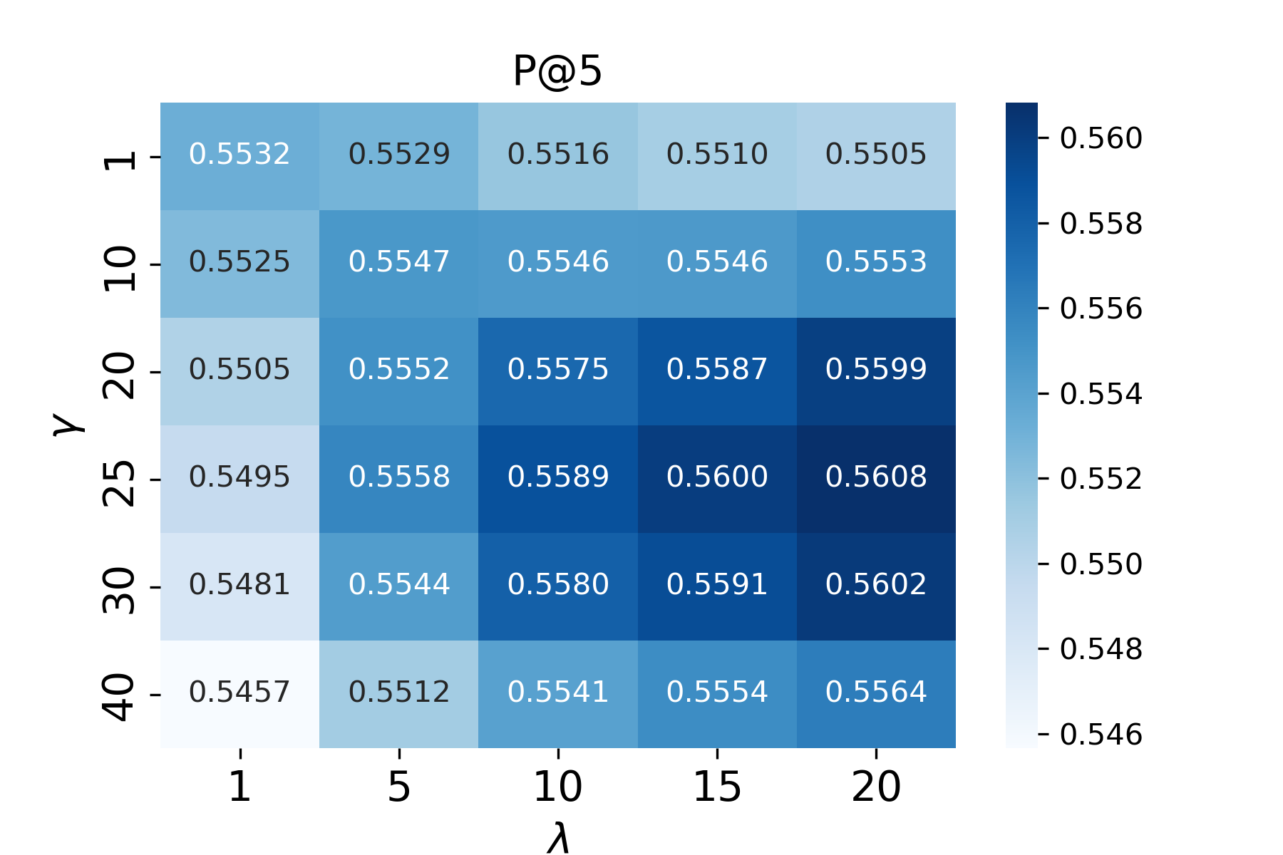
(a) Precision@5

(b) Recall@5

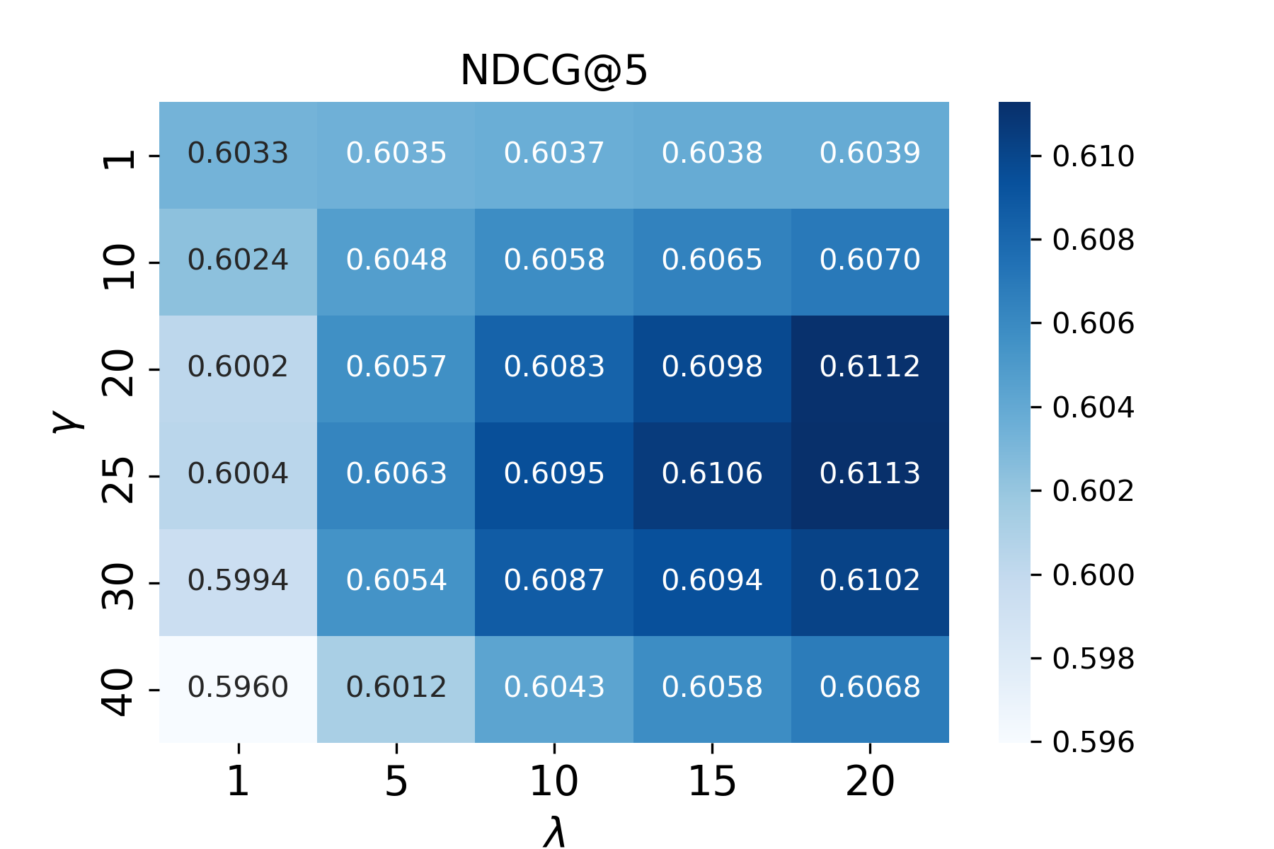
(c) NDCG@5

Figure 3: Effect of $\lambda$ and $\gamma$ on synthetic dataset with $\tau=0.5$

A.4 Experiments on the doubly robust estimators.

The doubly robust (DR) estimator Jiang and Li (2016), which is a hybrid of direct method (DM) estimator and inverse propensity score (IPS) estimator, is also widely used for off-policy evaluation. More specifically, let $\hat{\eta}:\mathcal{X}\times\mathcal{A}\rightarrow R$ be the imputation model in DM that estimates the reward of action $a$ under context vector $\bm{x}$, and $\hat{\beta}(a|\bm{x})$ be the estimated logging policy in the IPS estimator. The DR estimator evaluates policy $\pi$ based on the logged dataset $D:=\{(\bm{x}_{n},a_{n},r_{\bm{x}_{n},a_{n}})|n\in[N]\},$ by:

$$\hat{V}_{\rm DR}(\pi)=\hat{V}_{\rm DM}(\pi)+\frac{1}{N}\sum_{n=1}^{N}\frac{\pi(a_{n}|\bm{x}_{n})}{\hat{\beta}(a_{n}|\bm{x}_{n})}\big{(}r_{\bm{x}_{n},a_{n}}-\hat{\eta}(\bm{x}_{n},a_{n})\big{)}$$ (10)

where $\hat{V}_{\rm DM}(\pi)$ is the DM estimator:

$$\hat{V}_{\rm DM}(\pi)=\frac{1}{N}\sum_{n=1}^{N}\sum_{a\in\mathcal{A}}\pi(a|\bm{x}_{n})\hat{\eta}(\bm{x}_{n},a).$$ (11)

Again assume the policy $\pi(a|\bm{x})$ is parameterized by $\bm{\vartheta}$, the REINFORCE gradient of $\hat{V}_{{\rm DR}}(\pi_{\bm{\vartheta}})$ with respect to $\bm{\vartheta}$ can be readily derived as follows:

$$\nabla_{\bm{\vartheta}}\hat{V}_{{\rm DR}}(\pi_{\bm{\vartheta}})= \frac{1}{N}\sum_{n=1}^{N}\left(\sum_{a\in\mathcal{A}}\pi_{\bm{\vartheta}}(a|\bm{x}_{n})\hat{\eta}(\bm{x}_{n},a)\nabla_{\bm{\vartheta}}\log(\pi_{\bm{\vartheta}}(a|\bm{x}_{n}))\right)$$

$$+\frac{1}{N}\sum_{n=1}^{N}\left(\frac{\pi(a_{n}|\bm{x}_{n})}{\hat{\beta}(a_{n}|\bm{x}_{n})}\big{(}r_{\bm{x}_{n},a_{n}}-\hat{\eta}(\bm{x}_{n},a_{n})\big{)}\nabla_{\bm{\vartheta}}\log(\pi_{\bm{\vartheta}}(a_{n}|\bm{x}_{n})\right).$$ (12)

The imputation model $\hat{\eta}(\bm{x},a)$ is pre-trained following previous work Liu et al. (2022) with the same neural network architecture as the logging policy model. Besides the standard DR estimator, we also adapt UIPS and the best two baselines on off-policy evaluation estimator (i.e., MinVar and Shrinkage based on the results in Table 2 and Table 4) to doubly robust setting using the same imputation model.

Table 8 and Table 8 report the empirical performance of the learned policy on the synthetic datasets and three real-world datasets respectively. For ease of comparison, we also include the experiment results of BIPS-Cap and UIPS on each dataset in these two tables. Two $p$-values are also provided: (1) $p$-value (UIPSDR): The $p$-value under the t-test between UIPSDR and the best DR baseline on each dataset; (2) $p$-value (UIPS): The $p$-value under the t-test between UIPS and the best DR baseline on each dataset. From Table 8 and Table 8, we can first observe that DR cannot consistently outperform BIPS-Cap: It outperformed BIPS-Cap on the Coat and KuaiRec dataset, while achieving much worse performance on the synthetic datasets and Yahoo dataset. This is because the imputation model also plays a very important role in gradient calculation as shown in Eq.(12). Its accuracy greatly affects policy learning. When the imputation model is sufficiently accurate, for example, on the Coat dataset with only $300$ actions, incorporating the DM estimator not only led to better performance of DR over IPS, but also improved performance of UIPSDR over UIPS. And in particular, in this situation UIPSDR performed better than DR with the gain being statistically significant. When the imputation model is not accurate enough, for example, on the KuaiRec dataset with a large action space but sparse reward feedback, DR is still worse than UIPS, and UIPSDR also performs worse than UIPS due to the distortion of the imputation model.

Table 7: Experiment results on synthetic datasets. The best and second best results are highlighted with bold and underline respectively. Two $p$-values are calculated: (1) $p$-value (UIPSDR): The $p$-value under the t-test between UIPSDR and the best DR baseline on each dataset; (2) $p$-value (UIPS): The $p$-value under the t-test between UIPS and the best DR baseline on each dataset.

	$\tau=0.5$			$\tau=1$			$\tau=2$
Algorithm	P@5	R@5	NDCG@5	P@5	R@5	NDCG@5	P@5	R@5	NDCG@5
BIPS-Cap	0.5515$\pm 2e^{-3}$	0.1553 $\pm 8e^{-4}$	0.6031$\pm 2e^{-3}$	0.5526$\pm 2e^{-3}$	0.1561$\pm 6e^{-4}$	0.6016$\pm 1e^{-3}$	0.5409$\pm 3e^{-3}$	0.1529$\pm 9e^{-4}$	0.5901$\pm 2e^{-3}$
UIPS	0.5589$\pm 3e^{-3}$	0.1583$\pm 9e^{-4}$	0.6095$\pm 3e^{-3}$	0.5572$\pm 2e^{-3}$	0.1571$\pm 8e^{-4}$	0.6074$\pm 2e^{-3}$	0.5432$\pm 3e^{-3}$	0.1534$\pm 8e^{-4}$	0.5946$\pm 2e^{-3}$
DR	0.3846$\pm 3e^{-2}$	0.1082$\pm 8e^{-3}$	0.4684$\pm 3e^{-2}$	0.3631$\pm 3e^{-2}$	0.1017$\pm 9e^{-3}$	0.4494$\pm 3e^{-2}$	0.3560$\pm 3e^{-2}$	0.0995$\pm 7e^{-3}$	0.4470$\pm 2e^{-3}$
MinVarDR	0.3212$\pm 3e^{-2}$	0.0908$\pm 8e^{-3}$	0.4062$\pm 3e^{-2}$	0.3240$\pm 5e^{-2}$	0.0903$\pm 1e^{-2}$	0.3905$\pm 5e^{-2}$	0.3234$\pm 5e^{-2}$	0.0910$\pm 1e^{-2}$	0.4059$\pm 4e^{-2}$
ShrinkageDR	0.4139$\pm 2e^{-2}$	0.1161$\pm 7e^{-3}$	0.4969$\pm 3e^{-2}$	0.3944$\pm 3e^{-2}$	0.1101$\pm 8e^{-3}$	0.4797$\pm 2e^{-2}$	0.4080$\pm 3e^{-2}$	0.1135$\pm 7e^{-3}$	0.4901$\pm 2e^{-2}$
UIPSDR	0.4278$\pm 2e^{-2}$	0.1200$\pm 6e^{-3}$	0.5069$\pm 2e^{-2}$	0.4008$\pm 2e^{-2}$	0.1126$\pm 7e^{-3}$	0.4847$\pm 2e^{-2}$	0.4144$\pm 2e^{-2}$	0.1162$\pm 8e^{-3}$	0.4972$\pm 2e^{-2}$
$p$-value (UIPSDR)	$2e^{-1}$	$2e^{-1}$	$3e^{-1}$	$6e^{-1}$	$4e^{-1}$	$6e^{-1}$	$6e^{-1}$	$4e^{-1}$	$5e^{-1}$
$p$-value (UIPS)	$6e^{-13}$	$4e^{-13}$	$4e^{-12}$	$2e^{-12}$	$1e^{-12}$	$5e^{-12}$	$8e^{-12}$	$8e^{-12}$	$2e^{-11}$

Table 8: Experiment results on real-world unbiased datasets. The best and second best results are highlighted with bold and underline respectively. Two $p$-values are calculated: (1) $p$-value (UIPSDR): The $p$-value under the t-test between UIPSDR and the best DR baseline on each dataset; (2) $p$-value (UIPS): The $p$-value under the t-test between UIPS and the best DR baseline on each dataset.

	Yahoo			Coat			KuaiRec
Algorithm	P@5	R@5	NDCG@5	P@5	R@5	NDCG@5	P@50	R@50	NDCG@50
BIPS-Cap	0.2808$\pm 2e^{-3}$	0.7576$\pm 5e^{-3}$	0.6099$\pm 8e^{-3}$	0.2758$\pm 6e^{-3}$	0.4582$\pm 7e^{-3}$	0.4399$\pm 9e^{-3}$	0.8750$\pm 3e^{-3}$	0.0238$\pm 7e^{-5}$	0.8788$\pm 5e^{-3}$
UIPS	0.2868$\pm 2e^{-3}$	0.7742$\pm 5e^{-3}$	0.6274$\pm 5e^{-3}$	0.2877$\pm 3e^{-3}$	0.4757$\pm 5e^{-3}$	0.4576$\pm 8e^{-3}$	0.9120$\pm 1e^{-3}$	0.0250$\pm 5e^{-5}$	0.9174$\pm 7e^{-4}$
DR	0.2670$\pm 2e^{-3}$	0.7174$\pm 6e^{-3}$	0.5636$\pm 6e^{-3}$	0.2884$\pm 3e^{-3}$	0.4760$\pm 5e^{-3}$	0.4541$\pm 5e^{-3}$	0.8794$\pm 1e^{-2}$	0.0240$\pm 5e^{-4}$	0.8824$\pm 2e^{-2}$
MinVarDR	0.2272$\pm 5e^{-3}$	0.5989$\pm 1e^{-2}$	0.4525$\pm 1e^{-2}$	0.2704$\pm 4e^{-3}$	0.4434$\pm 9e^{-3}$	0.4137$\pm 6e^{-3}$	0.8640$\pm 7e^{-3}$	0.0235$\pm 2e^{-4}$	0.8657$\pm 7e^{-3}$
ShrinkageDR	0.2697$\pm 2e^{-3}$	0.7226$\pm 6e^{-3}$	0.5713$\pm 5e^{-3}$	0.2895$\pm 4e^{-3}$	0.4749$\pm 6e^{-3}$	0.4526$\pm 6e^{-3}$	0.8778$\pm 2e^{-2}$	0.0239$\pm 5e^{-4}$	0.8800$\pm 2e^{-2}$
UIPSDR	0.2721$\pm 1e^{-3}$	0.7294$\pm 6e^{-3}$	0.5750$\pm 5e^{-3}$	0.2946$\pm 4e^{-3}$	0.4854$\pm 8e^{-3}$	0.4647$\pm 8e^{-3}$	0.8849$\pm 1e^{-2}$	0.0242$\pm 4e^{-4}$	0.8896$\pm 1e^{-2}$
$p$-value (UIPSDR)	$1e^{-2}$	$2e^{-2}$	$1e^{-1}$	$7e^{-3}$	$5e^{-3}$	$2e^{-3}$	$4e^{-1}$	$4e^{-1}$	$3e^{-1}$
$p$-value (UIPS)	$1e^{-12}$	$6e^{-14}$	$6e^{-15}$	$3e^{-1}$	$8e^{-1}$	$1e^{-1}$	$2e^{-6}$	$2e^{-6}$	$1e^{-3}$

A.5 Difference against DICE-type algorithms.

The DICE line of work Nachum et al. (2019); Zhang et al. (2020); Dai et al. (2020) is proposed for off-policy correction in the multi-step RL setting with the environment following the Markov Decision Process (MDP) assumption. Although the DICE line of work does not require the knowledge of the logging policy, it is fundamentally different from our work. Given a logged dataset $D:=\{(s_{t},a_{t},r_{s_{t},a_{t}},s_{t+1})\}$ collected from an unknown logging policy $\beta^{*}(a_{t}|s_{t})$, DICE-type algorithms propose to directly estimate the discounted stationary distribution correction $w_{\pi/D}(s_{t},a_{t})=\frac{d^{\pi}(s_{t},a_{t})}{d^{D}(s_{t},a_{t})}$ to replace the product-based off-policy correction weight $\prod_{t}\frac{\pi(a_{t}|s_{t})}{\beta^{*}(a_{t}|s_{t})}$, which suffers high variance due to the series of products. While the estimation of $w_{\pi/D}(s_{t},a_{t})$ is agnostic to the logging policy, it highly depends on two assumptions: (1) Environment follows an MDP, i.e., $s_{t+1}\sim T(s_{t},a_{t})$ with $T(\cdot,\cdot)$ denoting the state transition function; (2) Each logged sample should be of a state-action-next-state tuple $(s_{t},a_{t},r_{s_{t},a_{t}},s_{t+1})$ that contains state transition information.

We further inspected how DICE-type algorithms would work in the contextual bandit setting, which can be taken as a one-state MDP. We take DualDICE [1] as an example for illustration, and similar conclusions can be drawn for other DICE-type algorithms. We can easily derive that in the contextual bandit setting, DualDICE degenerates to the IPS estimator that approximates the unknown ground-truth logging policy $\beta^{*}(a|s)$ with its empirical estimate from the given logged dataset $D:=\{(s_{i},a_{i},r_{s_{i},a_{i}})|i\in[N]\}$, which inherits all limitations of IPS estimator, such as high variance on instances with low support in $D$.

More specifically, recall that DualDICE estimates the discounted stationary distribution correction by optimizing the following objective function (Eq.(8) in Nachum et al. (2019)):

$$\min_{x:S\times A\rightarrow C}\quad\frac{1}{2}E_{(s,a)\sim d^{D}}[x(s,a)^{2}]-E_{(s,a)\sim d^{\pi}}[x(s,a)],$$

with the optimizer $x^{*}(s,a)=w_{\pi/D}(s,a)$. In a multi-step RL setting, one cannot directly calculate the second expectation as $d^{\pi}(s,a)$ is inaccessible, thus DualDICE takes the change-of-variable trick to address the above optimization problem. However, in the contextual bandit setting, let $p(s)$ denote the state distribution, $d^{\pi}(s,a)=p(s)\pi(a|s)$ and $d^{D}(s,a)=p(s)\beta^{*}(a|s)$. The optimization problem can be rewritten as :

$$\qquad\qquad\min_{x:S\times A\rightarrow C}\quad E_{s\sim p(s)}\left[\frac{1}{2}E_{a\sim\beta^{*}(a|s)}[x(s,a)^{2}]-E_{a\sim\pi(a|s)}[x(s,a)]\right].$$

With the logged dataset $D$, the empirical estimate of above optimization problem is :

$$\qquad\qquad\min_{x:S\times A\rightarrow C}\quad\sum_{s}\frac{N_{s}}{N}\left(\sum_{a}\frac{N_{s,a}}{2N_{s}}x(s,a)^{2}-\sum_{a}\pi(a|s)x(s,a)\right),$$

yielding $x^{*}(s,a)=\pi(a|s)N_{s}/N_{s,a}$, where $N_{s}$ and $N_{s,a}$ denote the number of logged samples with $s_{i}=s$ and ($s_{i}=s,a_{i}=a$) respectively. This is actually equivalent to the IPS estimator with $N_{s,a}/N_{s}$ as the estimate of $\beta^{*}(a|s)$. We refer to the above estimator as DICE-S, and Table 10 and Table 10 show the empirical performance of the policy learned through DICE-S on the synthetic and real-world datasets respectively. Similar as BIPS-Cap described in Section 4, we also clip propensity scores to control variance. One can observe from Table 10 and Table 10 that DICE-S performs worse than BIPS-Cap in all datasets except the KuaiRec dataset. Additionally, DICE-S underperforms compared to UIPS in all datasets. This is due to the fact that although DICE-S is unbiased, it only becomes accurate with numerous logged samples, and suffers high variance when logged samples are limited, resulting in its poor performance in our experiments.

Table 9: Empirical performance of DICE-S on synthetic datasets.

	$\tau=0.5$			$\tau=1$			$\tau=2$
Algorithm	P@5	R@5	NDCG@5	P@5	R@5	NDCG@5	P@5	R@5	NDCG@5
BIPS-Cap	0.5515$\pm 2e^{-3}$	0.1553 $\pm 8e^{-4}$	0.6031$\pm 2e^{-3}$	0.5526$\pm 2e^{-3}$	0.1561$\pm 6e^{-4}$	0.6016$\pm 1e^{-3}$	0.5409$\pm 3e^{-3}$	0.1529$\pm 9e^{-4}$	0.5901$\pm 2e^{-3}$
DICE-S	0.5416$\pm 4e^{-3}$	0.1520 $\pm 1e^{-3}$	0.5968$\pm 4e^{-3}$	0.5508$\pm 2e^{-3}$	0.1553$\pm 7e^{-4}$	0.6010$\pm 2e^{-3}$	0.5403$\pm 2e^{-3}$	0.1526$\pm 7e^{-4}$	0.5903$\pm 1e^{-3}$
UIPS	0.5589$\pm 3e^{-3}$	0.1583$\pm 9e^{-4}$	0.6095$\pm 3e^{-3}$	0.5572$\pm 2e^{-3}$	0.1571$\pm 8e^{-4}$	0.6074$\pm 2e^{-3}$	0.5432$\pm 3e^{-3}$	0.1534$\pm 8e^{-4}$	0.5946$\pm 2e^{-3}$

Table 10: Empirical performance of DICE-S on real-world datasets.

	Yahoo			Coat			KuaiRec
Algorithm	P@5	R@5	NDCG@5	P@5	R@5	NDCG@5	P@50	R@50	NDCG@50
BIPS-Cap	0.2808$\pm 2e^{-3}$	0.7576$\pm 5e^{-3}$	0.6099$\pm 8e^{-3}$	0.2758$\pm 6e^{-3}$	0.4582$\pm 7e^{-3}$	0.4399$\pm 9e^{-3}$	0.8750$\pm 3e^{-3}$	0.0238$\pm 7e^{-5}$	0.8788$\pm 5e^{-3}$
DICE-S	0.2618$\pm 4e^{-3}$	0.7010 $\pm 1e^{-2}$	0.5627$\pm 9e^{-3}$	0.2686$\pm 5e^{-3}$	0.4422$\pm 6e^{-3}$	0.4265$\pm 5e^{-3}$	0.8842$\pm 2e^{-3}$	0.0241$\pm 6e^{-5}$	0.8908$\pm 2e^{-3}$
UIPS	0.2868$\pm 2e^{-3}$	0.7742$\pm 5e^{-3}$	0.6274$\pm 5e^{-3}$	0.2877$\pm 3e^{-3}$	0.4757$\pm 5e^{-3}$	0.4576$\pm 8e^{-3}$	0.9120$\pm 1e^{-3}$	0.0250$\pm 5e^{-5}$	0.9174$\pm 7e^{-4}$

A.6 Difference against distributionally robust off-policy evaluation and learning.

Our work is fundamentally different from the line of work on distributionally robust off-policy evaluation and learning Si et al. (2020); Kallus et al. (2022); Xu et al. (2022). This results in different objectives that guide the use of min-max optimization.

Specifically, the work in Si et al. (2020); Kallus et al. (2022); Xu et al. (2022) assumes unknown changes exist between their training and deployment environments, such as user preference drift or unforeseen events during policy execution. Thus they choose to maximize the policy value (e.g., $\hat{V}_{{\rm IPS}}(\pi)$) in the worst environment within an uncertainty set around the training environment,

$$\max_{\pi}\min_{\mathcal{U}}\quad\hat{V}_{{\rm IPS}}(\pi).$$

As a result, their uncertainty set is created by introducing a small perturbation to the training environment. For example, the work in  Si et al. (2020); Kallus et al. (2022) searches the worst environment $\mathcal{P_{1}}$ in the $\sigma$-close perturbed environments around the training environment $\mathcal{P}_{0}$ (Eq.(1) in Kallus et al. (2022)):

$$\mathcal{U}(\sigma)=\{\mathcal{P}_{1}:\mathcal{P}_{1}<<\mathcal{P}_{0}\quad\text{and}\quad D_{KL}(\mathcal{P}_{1}||\mathcal{P}_{0})\leq\sigma\}.$$

And the work in Xu et al. (2022) adversarially perturbs the known ground-truth logging policy $\pi_{0}(\cdot|\cdot)$ in searching for the worst case (Eq.(4) in Xu et al. (2022)):

$$\mathcal{U}(\alpha)=\{\pi_{u}:\max_{a,x}~{}~{}\max\{\frac{\pi_{u}(a|x)}{\pi_{0}(a|x)},\frac{\pi_{0}(a|x)}{\pi_{u}(a|x)}\}\leq e^{\alpha}\}.$$

In contrast, UIPS assumes the training and deployment environments stay the same, but the ground-truth logging policy is unknown. To control the high bias and high variance caused by inaccurately and small estimated logging probabilities, UIPS explicitly models the uncertainty in the estimated logging policy by incorporating a per-sample weight $\phi_{\bm{x},a}$ as discussed in Eq.(4). In order to make $\hat{V}_{{\rm UIPS}}(\pi_{\bm{\vartheta}})$ as accurate as possible despite the unknown ground-truth logging policy $\beta^{*}(\cdot|\cdot)$, UIPS solves a min-max optimization problem in Eq.(8). This optimization problem seeks to find the optimal $\phi_{\bm{x},a}$ that minimizes the upper bound of the mean squared error (MSE) of $\hat{V}_{{\rm UIPS}}$ to its ground-truth value, within an uncertainty set of the unknown ground-truth logging policy $\beta^{*}(\cdot|\cdot)$. The closed-form solution for the min-max optimization is also derived as in Theorem 3.2.

Furthermore, observing that work in Xu et al. (2022) also performs optimization over an uncertainty set of the logging policy, we further adapted their method to handle the inaccuracy of the estimated logging policy, by taking $\pi_{0}(\cdot|\cdot)$ as the estimated logging policy, i.e., $\pi_{0}(\cdot|\cdot)=\hat{\beta}(\cdot|\cdot)$. We name the adapted methods as IPS-UN. Table 11 demonstrates the performance of the learned policy under IPS-UN on three synthetic datasets. The results suggest that directly applying IPS-UN to handle inaccurately estimated logging probabilities is not be a feasible solution to our problem. One important reason for the worse performance of IPS-UN is that it strives to optimize for the worst potential environment, which might not be the case in our experiment datatsets. On the other hand, UIPS assumes the training and deployment environments stay same and strives to identify the optimal policy with an unknown ground-truth logging policy.

Table 11: Empirical performance of IPS-UN on synthetic datasets.

	$\tau=0.5$			$\tau=1$			$\tau=2$
Algorithm	P@5	R@5	NDCG@5	P@5	R@5	NDCG@5	P@5	R@5	NDCG@5
BIPS-Cap	0.5515$\pm 2e^{-3}$	0.1553 $\pm 8e^{-4}$	0.6031$\pm 2e^{-3}$	0.5526$\pm 2e^{-3}$	0.1561$\pm 6e^{-4}$	0.6016$\pm 1e^{-3}$	0.5409$\pm 3e^{-3}$	0.1529$\pm 9e^{-4}$	0.5901$\pm 2e^{-3}$
IPS-UN	0.4089$\pm 3e^{-2}$	0.1152 $\pm 8e^{-3}$	0.4916$\pm 2e^{-2}$	0.3911$\pm 3e^{-3}$	0.1100$\pm 9e^{-3}$	0.4754$\pm 3e^{-2}$	0.3599 $\pm 4e^{-2}$	0.1009$\pm 1e^{-2}$	0.4353$\pm 4e^{-2}$
UIPS	0.5589$\pm 3e^{-3}$	0.1583$\pm 9e^{-4}$	0.6095$\pm 3e^{-3}$	0.5572$\pm 2e^{-3}$	0.1571$\pm 8e^{-4}$	0.6074$\pm 2e^{-3}$	0.5432$\pm 3e^{-3}$	0.1534$\pm 8e^{-4}$	0.5946$\pm 2e^{-3}$

A.7 Theoretical Proofs.

Proof of Proposition 2.1:

Proof  Because of the linearity of expectation, we have $\mathbb{E}_{D}\left[\hat{V}_{{\rm BIPS}}(\pi_{\bm{\vartheta}})\right]=\mathbb{E}_{\beta^{*}}\left[\frac{\pi_{\bm{\vartheta}}(a|\bm{x})}{\hat{\beta}(a|\bm{x})}r_{\bm{x},a}\right]$, and thus:

$${\rm Bias\left(\hat{V}_{{\rm BIPS}}(\pi_{\bm{\vartheta}})\right)} =\mathbb{E}_{D}\left[\hat{V}_{{\rm BIPS}}(\pi_{\bm{\vartheta}})-V(\pi_{\bm{\vartheta}})\right]$$

$$=\mathbb{E}_{\beta^{*}}\left[\frac{\pi_{\bm{\vartheta}}(a|\bm{x})}{\hat{\beta}(a|\bm{x})}r_{\bm{x},a}\right]-\mathbb{E}_{\beta^{*}}\left[\frac{\pi_{\bm{\vartheta}}(a|\bm{x})}{\beta^{*}(a|\bm{x})}r_{\bm{x},a}\right]$$

$$=\mathbb{E}_{\beta^{*}}\left[\frac{\pi_{\bm{\vartheta}}(a|\bm{x})}{\beta^{*}(a|\bm{x})}r_{\bm{x},a}\left(\frac{\beta^{*}(a|\bm{x})}{\hat{\beta}(a|\bm{x})}-1\right)\right]$$

$$=\mathbb{E}_{\pi_{\bm{\vartheta}}}\left[r_{\bm{x},a}\left(\frac{\beta^{*}(a|\bm{x})}{\hat{\beta}(a|\bm{x})}-1\right)\right].$$ (13)

Since samples are independently sampled from logging policy, the variance can be computed as:

$${\rm Var}_{D}\left(\hat{V}_{{\rm BIPS}}(\pi_{\bm{\vartheta}})\right) =\frac{1}{N}{\rm Var}_{\beta^{*}}\left(\frac{\pi_{\bm{\vartheta}}(a|\bm{x})}{\hat{\beta}(a|\bm{x})}r_{\bm{x},a}\right).$$

By re-scaling, we get:

$$N\cdot{\rm Var}_{D}\left(\hat{V}_{{\rm BIPS}}(\pi_{\bm{\vartheta}})\right) ={\rm Var}_{\beta^{*}}\left(\frac{\pi_{\bm{\vartheta}}(a|\bm{x})}{\hat{\beta}(a|\bm{x})}r_{\bm{x},a}\right)$$ (14)

$$=\mathbb{E}_{\beta^{*}}\left[\frac{\pi_{\bm{\vartheta}}(a|\bm{x})^{2}}{\hat{\beta}(a|\bm{x})^{2}}r_{\bm{x},a}^{2}\right]-\left(\mathbb{E}_{\beta^{*}}\left[\frac{\pi_{\bm{\vartheta}}(a|\bm{x})}{\hat{\beta}(a|\bm{x})}r_{\bm{x},a}\right]\right)^{2}$$

$$=\mathbb{E}_{\pi_{\bm{\vartheta}}}\left[\frac{\pi_{\bm{\vartheta}}(a|\bm{x})}{\beta^{*}(a|\bm{x})}\cdot\frac{\beta^{*}(a|\bm{x})^{2}}{\hat{\beta}(a|\bm{x})^{2}}r_{\bm{x},a}^{2}\right]-\left(\mathbb{E}_{\pi_{\bm{\vartheta}}}\left[\frac{\beta^{*}(a|\bm{x})}{\hat{\beta}(a|\bm{x})}r_{\bm{x},a}\right]\right)^{2}$$

This completes the proof.  

Proof of Theorem 3.1:

Proof  We can get:

$${\rm MSE}\left(\hat{V}_{{\rm UIPS}}(\pi_{\bm{\vartheta}})\right) =\mathbb{E}_{D}\left[\left(\hat{V}_{{\rm UIPS}}(\pi_{\bm{\vartheta}})-V(\pi_{\bm{\vartheta}})\right)^{2}\right]$$

$$=\left(\mathbb{E}_{D}\left[\hat{V}_{{\rm UIPS}}(\pi_{\bm{\vartheta}})-V(\pi_{\bm{\vartheta}})\right]\right)^{2}+{\rm Var}_{D}\left(\hat{V}_{{\rm UIPS}}(\pi_{\bm{\vartheta}})-V(\pi_{\bm{\vartheta}})\right)$$

$$=\left(\mathbb{E}_{D}\left[\hat{V}_{{\rm UIPS}}(\pi_{\bm{\vartheta}})-V(\pi_{\bm{\vartheta}})\right]\right)^{2}+{\rm Var}_{D}\left(\hat{V}_{{\rm UIPS}}(\pi_{\bm{\vartheta}})\right)$$

$$={\rm Bias}(\hat{V}_{{\rm UIPS}}(\pi_{\bm{\vartheta}}))^{2}+{\rm Var}(\hat{V}_{{\rm UIPS}}(\pi_{\bm{\vartheta}})).$$

We first bound the bias term:

$${\rm Bias}(\hat{V}_{{\rm UIPS}}(\pi_{\bm{\vartheta}})) =\mathbb{E}_{D}\left[\hat{V}_{{\rm UIPS}}(\pi_{\bm{\vartheta}})-V(\pi_{\bm{\vartheta}})\right]$$

$$\stackrel{{\scriptstyle(1)}}{{=}}\mathbb{E}_{\beta^{*}}\left[\frac{\pi_{\bm{\vartheta}}(a|\bm{x})}{\hat{\beta}(a|\bm{x})}\phi_{\bm{x},a}r_{\bm{x},a}\right]-V(\pi_{\bm{\vartheta}})$$

$$=\mathbb{E}_{\beta^{*}}\left[\frac{\pi_{\bm{\vartheta}}(a|\bm{x})}{\hat{\beta}(a|\bm{x})}\phi_{\bm{x},a}r_{\bm{x},a}-\frac{\pi_{\bm{\vartheta}}(a|\bm{x})}{\beta^{*}(a|\bm{x})}r_{\bm{x},a}\right]$$

$$=\mathbb{E}_{\beta^{*}}\left[r_{\bm{x},a}\frac{\pi_{\bm{\vartheta}}(a|\bm{x})}{\beta^{*}(a|\bm{x})}\cdot\left(\frac{\beta^{*}(a|\bm{x})}{\hat{\beta}(a|\bm{x})}\phi_{\bm{x},a}-1\right)\right]$$

$$\stackrel{{\scriptstyle(2)}}{{\leq}}\sqrt{\mathbb{E}_{\pi_{\bm{\vartheta}}}\left[r_{\bm{x},a}^{2}\frac{\pi_{\bm{\vartheta}}(a|\bm{x})}{\beta^{*}(a|\bm{x})}\right]}\cdot\sqrt{\mathbb{E}_{\beta^{*}}\left[\left(\frac{\beta^{*}(a|\bm{x})}{\hat{\beta}(a|\bm{x})}\phi_{\bm{x},a}-1\right)^{2}\right]}$$

Step (1) follows the linearity of expectation and step (2) is due to the Cauchy-Schwarz inequality. We then bound the variance term:

$${\rm Var}(\hat{V}_{{\rm UIPS}}(\pi_{\bm{\vartheta}})) =\frac{1}{N}{\rm Var}_{\beta^{*}}\left(\frac{\pi_{\bm{\vartheta}}(a|\bm{x})}{\hat{\beta}(a|\bm{x})}\phi_{\bm{x},a}r_{\bm{x},a}\right)$$

$$=\frac{1}{N}\left(\mathbb{E}_{\beta^{*}}\left[\frac{\pi_{\bm{\vartheta}}(a|\bm{x})^{2}}{\hat{\beta}(a|\bm{x})^{2}}\phi_{\bm{x},a}^{2}r_{\bm{x},a}^{2}\right]-\left(\mathbb{E}_{\beta^{*}}\left[\frac{\pi_{\bm{\vartheta}}(a|\bm{x})}{\hat{\beta}(a|\bm{x})}\phi_{\bm{x},a}r_{\bm{x},a}\right]\right)^{2}\right)$$

$$\leq\frac{1}{N}\mathbb{E}_{\beta^{*}}\left[\frac{\pi_{\bm{\vartheta}}(a|\bm{x})^{2}}{\hat{\beta}(a|\bm{x})^{2}}\phi_{\bm{x},a}^{2}r_{\bm{x},a}^{2}\right]\leq\mathbb{E}_{\beta^{*}}\left[\frac{\pi_{\bm{\vartheta}}(a|\bm{x})^{2}}{\hat{\beta}(a|\bm{x})^{2}}\phi_{\bm{x},a}^{2}\right]$$

Combining the bound of bias and variance completes the proof.  

Proof of Theorem 3.2:

Proof  We first define several notations:

• $T(\phi_{\bm{x},a},\beta_{\bm{x},a})=\lambda\mathbb{E}_{\beta^{*}}\left[\left(\frac{\beta_{\bm{x},a}}{\hat{\beta}(a|\bm{x})}\phi_{\bm{x},a}-1\right)^{2}\right]+\mathbb{E}_{\beta^{*}}\left[\frac{\pi_{\bm{\vartheta}}(a|\bm{x})^{2}}{\hat{\beta}(a|\bm{x})^{2}}\phi_{\bm{x},a}^{2}\right]$.

• $\tilde{T}(\phi_{\bm{x},a})=\max_{\beta_{\bm{x},a}\in\bm{B}_{\bm{x},a}}T(\phi_{\bm{x},a},\beta_{\bm{x},a})$ denotes the maximum value of inner optimization problem.

• $T^{*}=\min_{\phi_{\bm{x},a}}\tilde{T}(\phi_{\bm{x},a})=\min_{\phi_{\bm{x},a}}\max_{\beta_{\bm{x},a}\in\bm{B}_{\bm{x},a}}T(\phi_{\bm{x},a},\beta_{\bm{x},a})$ denote the optimal min-max value. And $\phi_{\bm{x},a}^{*}=\operatorname*{arg\,min}_{\phi_{\bm{x},a}}\tilde{T}(\phi_{\bm{x},a})$ .

• $\bm{B}_{\bm{x},a}^{-}:=\frac{\hat{Z}\exp\left(-\gamma U_{\bm{x},a}\right)}{Z^{*}}\hat{\beta}(a|\bm{x})$, and $\bm{B}_{\bm{x},a}^{+}:=\frac{\hat{Z}\exp\left(\gamma U_{\bm{x},a}\right)}{Z^{*}}\hat{\beta}(a|\bm{x})$.

We first find the maximum value of the inner optimization problem, i.e., $\tilde{T}(\phi_{\bm{x},a})$ for any fixed $\phi_{\bm{x},a}$. And there are three cases shown in Figure 4:

Figure 4: Three cases for maximizing the inner optimization problem.

Case I: When $\frac{\hat{\beta}(a|\bm{x})}{\phi_{\bm{x},a}}\geq\bm{B}_{\bm{x},a}^{+}$, , $\tilde{T}(\phi_{\bm{x},a})$ achieves the maximum value at $\beta_{\bm{x},a}=\bm{B}_{\bm{x},a}^{-}$. In other words, $\tilde{T}(\phi_{\bm{x},a})=T(\phi_{\bm{x},a},\bm{B}_{\bm{x},a}^{-})$ when $\phi_{\bm{x},a}\leq\frac{\hat{\beta}(a|\bm{x})}{\bm{B}_{\bm{x},a}^{+}}$.

Case II: When $\bm{B}_{\bm{x},a}^{-}\leq\frac{\hat{\beta}(a|\bm{x})}{\phi_{\bm{x},a}}\leq\bm{B}_{\bm{x},a}^{+}$, i.e., $\frac{Z^{*}\exp(-\gamma U_{\bm{x},a})}{\hat{Z}}\leq\phi_{\bm{x},a}\leq\frac{Z^{*}\exp(\gamma U_{\bm{x},a})}{\hat{Z}}$, then $\tilde{T}(\phi_{\bm{x},a})$ will be the maximum between $T(\phi_{\bm{x},a},\bm{B}_{\bm{x},a}^{-})$ and $T(\phi_{\bm{x},a},\bm{B}_{\bm{x},a}^{+})$.

More specifically, when $\frac{\hat{\beta}(a|\bm{x})}{\phi_{\bm{x},a}}\leq\frac{\bm{B}_{\bm{x},a}^{+}+\bm{B}_{\bm{x},a}^{-}}{2}$, i.e., $\phi_{\bm{x},a}\geq\frac{2\hat{\beta}(a|\bm{x})}{\bm{B}_{\bm{x},a}^{+}+\bm{B}_{\bm{x},a}^{-}}$, $\tilde{T}(\phi_{\bm{x},a})=T(\phi_{\bm{x},a},\bm{B}_{\bm{x},a}^{+})$. Otherwise when $\phi_{\bm{x},a}<\frac{2\hat{\beta}(a|\bm{x})}{\bm{B}_{\bm{x},a}^{+}+\bm{B}_{\bm{x},a}^{-}}$, $\tilde{T}(\phi_{\bm{x},a})=T(\phi_{\bm{x},a},\bm{B}_{\bm{x},a}^{-})$.

Case III: When $\phi_{\bm{x},a}\geq\frac{\hat{\beta}(a|\bm{x})}{\bm{B}_{\bm{x},a}^{-}}$. implying $\frac{\hat{\beta}(a|\bm{x})}{\phi_{\bm{x},a}}\leq\bm{B}_{\bm{x},a}^{-}$, $\tilde{T}(\phi_{\bm{x},a})=T(\phi_{\bm{x},a},\bm{B}_{\bm{x},a}^{+})$.

Overall, we get that:

$$\tilde{T}(\phi_{\bm{x},a})=\left\{\begin{array}[]{cc}T(\phi_{\bm{x},a},\bm{B}_{\bm{x},a}^{-}),&\phi_{\bm{x},a}\in(-\infty,\frac{2\hat{\beta}(a|\bm{x})}{\bm{B}_{\bm{x},a}^{+}+\bm{B}_{\bm{x},a}^{-}}]\\ T(\phi_{\bm{x},a},\bm{B}_{\bm{x},a}^{+})&\phi_{\bm{x},a}\in[\frac{2\hat{\beta}(a|\bm{x})}{\bm{B}_{\bm{x},a}^{+}+\bm{B}_{\bm{x},a}^{-}},\infty)\end{array}\right.$$ (15)

Next we try to find the minimum value of $\tilde{T}(\phi_{\bm{x},a})$. We first observe that without considering constraint on $\phi_{\bm{x},a}$, when

$$\phi_{\bm{x},a}^{+}=\frac{\lambda}{\lambda\frac{\bm{B}_{\bm{x},a}^{+}}{\hat{\beta}(a|\bm{x})}+\frac{\pi_{\bm{\vartheta}}(a|\bm{x})^{2}}{\hat{\beta}(a|\bm{x})\bm{B}_{\bm{x},a}^{+}}}$$

$T(\phi_{\bm{x},a},\bm{B}_{\bm{x},a}^{+})$ achieves the global minimum value. However, $\phi_{\bm{x},a}^{+}\leq\frac{\hat{\beta}(a|\bm{x})}{\bm{B}_{\bm{x},a}^{+}}\leq\frac{2\hat{\beta}(a|\bm{x})}{\bm{B}_{\bm{x},a}^{+}+\bm{B}_{\bm{x},a}^{-}}$, which implies when $\phi_{\bm{x},a}\in\left[\frac{2\hat{\beta}(a|\bm{x})}{\bm{B}_{\bm{x},a}^{+}+\bm{B}_{\bm{x},a}^{-}},\infty\right)$, the minimum value of $T(\phi_{\bm{x},a},\bm{B}_{\bm{x},a}^{+})$ is achieved at $\frac{2\hat{\beta}(a|\bm{x})}{\bm{B}_{\bm{x},a}^{+}+\bm{B}_{\bm{x},a}^{-}}$.

On the other hand, without considering any constraint on $\phi_{\bm{x},a}$ , the global minimum value of $T(\phi_{\bm{x},a},\bm{B}_{\bm{x},a}^{-})$ is achieved at:

$$\phi_{\bm{x},a}^{-}=\frac{\lambda}{\lambda\frac{\bm{B}_{\bm{x},a}^{-}}{\hat{\beta}(a|\bm{x})}+\frac{\pi_{\bm{\vartheta}}(a|\bm{x})^{2}}{\hat{\beta}(a|\bm{x})\bm{B}_{\bm{x},a}^{-}}}.$$ (16)

Thus if $\phi_{\bm{x},a}^{-}\leq\frac{2\hat{\beta}(a|\bm{x})}{\bm{B}_{\bm{x},a}^{+}+\bm{B}_{\bm{x},a}^{-}}$, $\phi_{\bm{x},a}^{*}=\phi_{\bm{x},a}^{-}$, since $T(\phi_{\bm{x},a}^{-},\bm{B}_{\bm{x},a}^{-})\leq T(\frac{2\hat{\beta}(a|\bm{x})}{\bm{B}_{\bm{x},a}^{+}+\bm{B}_{\bm{x},a}^{-}},\bm{B}_{\bm{x},a}^{-})=T(\frac{2\hat{\beta}(a|\bm{x})}{\bm{B}_{\bm{x},a}^{+}+\bm{B}_{\bm{x},a}^{-}},\bm{B}_{\bm{x},a}^{+})$. Otherwise, when $\phi_{\bm{x},a}\in(-\infty,\frac{2\hat{\beta}(a|\bm{x})}{\bm{B}_{\bm{x},a}^{+}+\bm{B}_{\bm{x},a}^{-}}]$, the minimum value of $T(\phi_{\bm{x},a},\bm{B}_{\bm{x},a}^{-})$ is also achieved at $\frac{2\hat{\beta}(a|\bm{x})}{\bm{B}_{\bm{x},a}^{+}+\bm{B}_{\bm{x},a}^{-}}$, implying $\phi_{\bm{x},a}^{*}=\frac{2\hat{\beta}(a|\bm{x})}{\bm{B}_{\bm{x},a}^{+}+\bm{B}_{\bm{x},a}^{-}}$.

Overall,

$$\phi_{\bm{x},a}^{*}=\min\left(\frac{\lambda}{\lambda\frac{\bm{B}_{\bm{x},a}^{-}}{\hat{\beta}(a|\bm{x})}+\frac{\pi_{\bm{\vartheta}}(a|\bm{x})^{2}}{\hat{\beta}(a|\bm{x})\bm{B}_{\bm{x},a}^{-}}},\frac{2\hat{\beta}(a|\bm{x})}{\bm{B}_{\bm{x},a}^{+}+\bm{B}_{\bm{x},a}^{-}}\right)$$ (17)

Let $\eta=\frac{Z^{*}}{\hat{Z}}$, we can get

$$\phi_{\bm{x},a}^{*}=\min\left(\frac{\lambda}{\frac{\lambda}{\eta}\exp\left(-\gamma U_{\bm{x},a}\right)+\frac{\eta\pi_{\bm{\vartheta}}(a|\bm{x})^{2}}{\hat{\beta}(a|\bm{x})^{2}\exp\left(-\gamma U_{\bm{x},a}\right)}},\frac{2\eta}{\exp\left(\gamma U_{\bm{x},a}\right)+\exp\left(-\gamma U_{\bm{x},a}\right)}\right).$$ (18)

Note that $\eta\in[\exp(-\gamma U_{s}^{\max}),\exp(\gamma U_{s}^{\max})]$, since $\hat{Z}\exp(-\gamma U_{s}^{\max})\leq Z^{*}=\sum_{a^{\prime}}\exp(f_{\theta^{*}}(a^{\prime}|\bm{x}))\leq\hat{Z}\exp(U_{s}^{\max})$.

This completes the proof .  

Proof of Corollary  3.3:

Proof  Following the similar procedure as in Theorem 3.1, we can derive the mean squared error (${\rm MSE}$) between $\hat{V}_{{\rm BIPS}}(\pi_{\bm{\vartheta}})$ and ground-truth estimator $V(\pi_{\bm{\vartheta}})$ is upper bounded as follows:

$${\rm MSE}\left(\hat{V}_{{\rm BIPS}}(\pi_{\bm{\vartheta}})\right) =\mathbb{E}_{D}\left[\left(\hat{V}_{{\rm BIPS}}(\pi_{\bm{\vartheta}})-V(\pi_{\bm{\vartheta}})\right)^{2}\right]$$

$$\leq\mathbb{E}_{\pi_{\bm{\vartheta}}}\left[r_{\bm{x},a}^{2}\frac{\pi_{\bm{\vartheta}}(a|\bm{x})}{\beta^{*}(a|\bm{x})}\right]\cdot\mathbb{E}_{\beta^{*}}\left[\left(\frac{\beta^{*}(a|\bm{x})}{\hat{\beta}(a|\bm{x})}-1\right)^{2}\right]+\mathbb{E}_{\beta^{*}}\left[\frac{\pi_{\bm{\vartheta}}(a|\bm{x})^{2}}{\hat{\beta}(a|\bm{x})^{2}}\right].$$

When $\beta^{*}(a|\bm{x})\in[\bm{B}_{\bm{x},a}^{-},\bm{B}_{\bm{x},a}^{+}]$, with $\bm{B}_{\bm{x},a}^{-}:=\frac{\hat{Z}\exp\left(-\gamma U_{\bm{x},a}\right)}{Z^{*}}\hat{\beta}(a|\bm{x})$ and $\bm{B}_{\bm{x},a}^{+}:=\frac{\hat{Z}\exp\left(\gamma U_{\bm{x},a}\right)}{Z^{*}}\hat{\beta}(a|\bm{x})$, ${\rm MSE}\left(\hat{V}_{{\rm BIPS}}(\pi_{\bm{\vartheta}})\right)$ can be further upper bounded as follows.

For ease of illustration, we set $\lambda=\mathbb{E}_{\pi_{\bm{\vartheta}}}\left[r_{\bm{x},a}^{2}\frac{\pi_{\bm{\vartheta}}(a|\bm{x})}{\beta^{*}(a|\bm{x})}\right]$ and

$$T(\phi_{\bm{x},a},\beta_{\bm{x},a})=\lambda\mathbb{E}_{\beta^{*}}\left[\left(\frac{\beta_{\bm{x},a}}{\hat{\beta}(a|\bm{x})}\phi_{\bm{x},a}-1\right)^{2}\right]+\mathbb{E}_{\beta^{*}}\left[\frac{\pi_{\bm{\vartheta}}(a|\bm{x})^{2}}{\hat{\beta}(a|\bm{x})^{2}}\phi_{\bm{x},a}^{2}\right].$$

Let $T^{*}_{{\rm BIPS}}$ denote the upper bound of ${\rm MSE}\left(\hat{V}_{{\rm BIPS}}(\pi_{\bm{\vartheta}})\right)$, then we can derive that

$$T^{*}_{{\rm BIPS}}=\left\{\begin{array}[]{cc}T(1,\bm{B}_{\bm{x},a}^{+}),&\hat{\beta}(a|\bm{x})\leq\frac{\bm{B}_{\bm{x},a}^{+}+\bm{B}_{\bm{x},a}^{-}}{2}\\ T(1,\bm{B}_{\bm{x},a}^{-}),&\hat{\beta}(a|\bm{x})>\frac{\bm{B}_{\bm{x},a}^{+}+\bm{B}_{\bm{x},a}^{-}}{2}.\end{array}\right.$$ (19)

Recall that in Theorem 3.2, we show that the upper bound of ${\rm MSE}\left(\hat{V}_{{\rm UIPS}}(\pi_{\bm{\vartheta}})\right)$ is as follows:

$$T^{*}_{{\rm UIPS}}=\left\{\begin{array}[]{lc}T(\phi_{\bm{x},a}^{-},\bm{B}_{\bm{x},a}^{-}),&\phi_{\bm{x},a}^{-}<\frac{2\hat{\beta}(a|\bm{x})}{\bm{B}_{\bm{x},a}^{+}+\bm{B}_{\bm{x},a}^{-}}\\ T(\frac{2\hat{\beta}(a|\bm{x})}{\bm{B}_{\bm{x},a}^{+}+\bm{B}_{\bm{x},a}^{-}},\bm{B}_{\bm{x},a}^{+}),&\phi_{\bm{x},a}^{-}\geq\frac{2\hat{\beta}(a|\bm{x})}{\bm{B}_{\bm{x},a}^{+}+\bm{B}_{\bm{x},a}^{-}}.\end{array}\right.$$ (20)

where $\phi_{\bm{x},a}^{-}$ is defined in Eq.(16). Next we show that $T^{*}_{{\rm UIPS}}\geq T^{*}_{{\rm BIPS}}$.

• When $\hat{\beta}(a|\bm{x})\leq\frac{\bm{B}_{\bm{x},a}^{+}+\bm{B}_{\bm{x},a}^{-}}{2}$, we can get $T^{*}_{{\rm BIPS}}=T(1,\bm{B}_{\bm{x},a}^{+})$ and $\frac{2\hat{\beta}(a|\bm{x})}{\bm{B}_{\bm{x},a}^{+}+\bm{B}_{\bm{x},a}^{-}}\leq 1$. If $\phi_{\bm{x},a}^{-}<\frac{2\hat{\beta}(a|\bm{x})}{\bm{B}_{\bm{x},a}^{+}+\bm{B}_{\bm{x},a}^{-}}$, then $T^{*}_{{\rm UIPS}}=T(\phi_{\bm{x},a}^{-},\bm{B}_{\bm{x},a}^{-})<T(\frac{2\hat{\beta}(a|\bm{x})}{\bm{B}_{\bm{x},a}^{+}+\bm{B}_{\bm{x},a}^{-}},\bm{B}_{\bm{x},a}^{-})=T(\frac{2\hat{\beta}(a|\bm{x})}{\bm{B}_{\bm{x},a}^{+}+\bm{B}_{\bm{x},a}^{-}},\bm{B}_{\bm{x},a}^{+})\leq T(1,\bm{B}_{\bm{x},a}^{+})$. And if $\phi_{\bm{x},a}^{-}\geq\frac{2\hat{\beta}(a|\bm{x})}{\bm{B}_{\bm{x},a}^{+}+\bm{B}_{\bm{x},a}^{-}}$, $T^{*}_{{\rm UIPS}}=T(\frac{2\hat{\beta}(a|\bm{x})}{\bm{B}_{\bm{x},a}^{+}+\bm{B}_{\bm{x},a}^{-}},\bm{B}_{\bm{x},a}^{+})\leq T(1,\bm{B}_{\bm{x},a}^{+})$;

• When $\hat{\beta}(a|\bm{x})>\frac{\bm{B}_{\bm{x},a}^{+}+\bm{B}_{\bm{x},a}^{-}}{2}$, we can get $T^{*}_{{\rm BIPS}}=T(1,\bm{B}_{\bm{x},a}^{-})$ and $\frac{2\hat{\beta}(a|\bm{x})}{\bm{B}_{\bm{x},a}^{+}+\bm{B}_{\bm{x},a}^{-}}>1$. If $\phi_{\bm{x},a}^{-}<\frac{2\hat{\beta}(a|\bm{x})}{\bm{B}_{\bm{x},a}^{+}+\bm{B}_{\bm{x},a}^{-}}$, then $T^{*}_{{\rm UIPS}}=T(\phi_{\bm{x},a}^{-},\bm{B}_{\bm{x},a}^{-})\leq T(1,\bm{B}_{\bm{x},a}^{-})$, since $\phi_{\bm{x},a}^{-}$ is a global minimum. Otherwise when $\phi_{\bm{x},a}^{-}\geq\frac{2\hat{\beta}(a|\bm{x})}{\bm{B}_{\bm{x},a}^{+}+\bm{B}_{\bm{x},a}^{-}}>1$, $T^{*}_{{\rm UIPS}}=T(\frac{2\hat{\beta}(a|\bm{x})}{\bm{B}_{\bm{x},a}^{+}+\bm{B}_{\bm{x},a}^{-}},\bm{B}_{\bm{x},a}^{+})=T(\frac{2\hat{\beta}(a|\bm{x})}{\bm{B}_{\bm{x},a}^{+}+\bm{B}_{\bm{x},a}^{-}},\bm{B}_{\bm{x},a}^{-})<T(1,\bm{B}_{\bm{x},a}^{-})$.

In both cases, we have $T^{*}_{{\rm UIPS}}\leq T^{*}_{{\rm BIPS}}$, thus completing the proof.

 

Lemma A.1

Under fixed $\pi_{\bm{\vartheta}}(a|\bm{x})$ and $\hat{\beta}(a|\bm{x})$, and $\alpha_{\bm{x},a}=\sqrt{\frac{\lambda}{2\eta^{2}}-\frac{\lambda(1-\eta)}{\eta^{2}}\exp(-2\gamma U_{\bm{x},a})}$, we have the following observations:

• If $\frac{\pi_{\bm{\vartheta}}(a|\bm{x})}{\hat{\beta}(a|\bm{x})}\leq\alpha_{\bm{x},a}$, $\phi_{\bm{x},a}^{*}=2\eta/\left[\exp(\gamma U_{\bm{x},a})+\exp(-\gamma U_{\bm{x},a})\right]$. Otherwise $\phi_{\bm{x},a}^{*}={\lambda}/\left[\frac{\lambda}{\eta}\exp\left(-\gamma U_{\bm{x},a}\right)+\frac{\eta\pi_{\bm{\vartheta}}(a|\bm{x})^{2}}{\hat{\beta}^{2}(a|\bm{x})\exp\left(-\gamma U_{\bm{x},a}\right)}]\right]$. In other words, $\phi_{\bm{x},a}^{*}\leq 2\eta$ always holds.

• If $\alpha_{\bm{x},a}\leq\frac{\pi_{\bm{\vartheta}}(a|\bm{x})}{\hat{\beta}(a|\bm{x})}$ and $\frac{\pi_{\bm{\vartheta}}(a|\bm{x})}{\bm{B}_{\bm{x},a}^{-}}<\sqrt{\lambda}$, larger $U_{\bm{x},a}$ brings larger $\phi_{\bm{x},a}^{*}$.

• Otherwise $\phi_{\bm{x},a}^{*}$ decreases as $U_{\bm{x},a}$ increases.

Proof  The following inequality validates the first observation:

$$\frac{\lambda}{\frac{\lambda}{\eta}\exp\left(-\gamma U_{\bm{x},a}\right)+\frac{\eta\pi_{\bm{\vartheta}}(a|\bm{x})^{2}}{\hat{\beta}^{2}(a|\bm{x})\exp\left(-\gamma U_{\bm{x},a}\right)}}\leq\frac{2\eta}{\exp\left(\gamma U_{\bm{x},a}\right)+\exp\left(-\gamma U_{\bm{x},a}\right)}$$

For the second and third observations, $\alpha_{\bm{x},a}\leq\frac{\sqrt{\lambda}}{\sqrt{2}\eta}\leq\frac{\sqrt{\lambda}}{\eta}$. Let $\mathcal{L}(u)=\frac{\lambda}{\eta}\exp(-\gamma u)+\frac{\eta\pi_{\bm{\vartheta}}(a|\bm{x})^{2}}{\hat{\beta}(a|\bm{x})^{2}\exp(-\gamma u)}$, we can have:

$$\nabla_{u}\mathcal{L}(u) =-\gamma\frac{\lambda}{\eta}\exp(-\gamma u)+\gamma\frac{\eta\pi_{\bm{\vartheta}}(a|\bm{x})^{2}}{\hat{\beta}(a|\bm{x})^{2}}\exp(\gamma u)$$

To make $\nabla_{u}\mathcal{L}(u)\geq 0$, we need $u\geq\frac{1}{\gamma}\log\left(\frac{\sqrt{\lambda}\hat{\beta}(a|\bm{x})}{\eta\pi_{\bm{\vartheta}}(a|\bm{x})}\right)$. This implies when $U_{\bm{x},a}\geq\frac{1}{\gamma}\log\left(\frac{\sqrt{\lambda}\hat{\beta}(a|\bm{x})}{\eta\pi_{\bm{\vartheta}}(a|\bm{x})}\right)$, $\phi_{\bm{x},a}^{*}$ will decrease as $U_{\bm{x},a}$ increases; otherwise as $U_{\bm{x},a}$ increases, $\phi_{\bm{x},a}^{*}$ also increases.

More specifically, when $\alpha_{\bm{x},a}\leq\frac{\pi_{\bm{\vartheta}}(a|\bm{x})}{\hat{\beta}(a|\bm{x})}$, we have:

$$U_{\bm{x},a}\leq\frac{1}{\gamma}\log\left(\frac{\sqrt{\lambda}\hat{\beta}(a|\bm{x})}{\eta\pi_{\bm{\vartheta}}(a|\bm{x})}\right)\Leftrightarrow\frac{\pi_{\bm{\vartheta}}(a|\bm{x})}{\bm{B}_{\bm{x},a}^{-}}<\sqrt{\lambda}\quad\Leftrightarrow\quad\frac{\pi_{\bm{\vartheta}}(a|\bm{x})}{\hat{\beta}(a|\bm{x})}<\frac{\sqrt{\lambda}}{\eta}\exp(-\gamma U_{\bm{x},a}).$$

In other words, for these samples, higher uncertainty implies smaller value of $\pi/\hat{\beta}$, and ${\rm UIPS}$ tends to boost such safe sample with higher $\phi_{\bm{x},a}^{*}$.

In other cases, $\phi_{\bm{x},a}^{*}$ decreases as $U_{\bm{x},a}$ increases. This completes the proof.  

A.8 Convergence Analysis

Next we provide the convergence analysis of policy improvement under UIPS.

Definition A.2

A function $f:\mathbb{R}^{d}\rightarrow\mathbb{R}$ is $L$-smooth when $\|\nabla f(x)-\nabla f(y)\|_{2}\leq L\|x-y\|_{2}$, for all $x,y\in\mathbb{R}^{d}$.

We first state and prove a general result, which serves as the basis to complete our convergence analysis of policy improvement under UIPS. The proof is a special case of convergence proof of stochastic gradient descent with biased gradients in Ajalloeian and Stich (2020). Suppose we have a differentiable function $f:\mathbb{R}^{d}\rightarrow\mathbb{R}$, which is $L$-smooth, and attains a finite minimum value $f^{*}:=\min_{x\in\mathbb{R}^{d}}f(x)$.

Suppose we cannot directly assess the gradient $\nabla f(x)$. Instead we can only assess a noisy but unbiased gradient $\zeta(x)\in\mathbb{R}^{d}$ at the given $x$ of the function $\tilde{f}(x)$.

Let $b(x)=\nabla\tilde{f}(x)-\nabla f(x)$ denote the difference between $\nabla\tilde{f}(x)$ and $\nabla f(x)$, and $\delta(x)=\zeta(x)-\nabla\tilde{f}(x)$ denote the noise in gradients. We assume that:

$$\|b(x)\|\leq\varphi\|\nabla f(x)\|\quad\text{and}\quad\mathbb{E}[\delta(x)]=0\quad\text{and}\quad\mathbb{E}[\|\delta(x)\|^{2}|x]\leq M\mathbb{E}[\|\nabla\tilde{f}(x)\|^{2}]+\sigma^{2}$$ (21)

where the constants $\varphi$ and $M$ satisfy $0<\varphi<1$ and $M\geq 0$ respectively. When running stochastic gradient descent algorithms, i.e. $x_{k+1}=x_{k}-\eta_{k}\zeta(x_{k})$, we have the following guarantee on the convergence of $x_{k}$ to an approximate stationary point of $f$.

Theorem A.3

Suppose $f(\cdot)$ is differentiable and $L$-smooth, and the assessed approximate gradient meets the conditions in Eq. equation 21 with parameters $(\sigma_{k},\varphi_{k})$ at iteration $k$. Denote $\sigma_{\max}=\max_{k}\sigma_{k}$ and $\varphi_{\max}=\max_{k}\varphi_{k}$. Set the stepsizes $\{\eta_{k}\}$ to $\eta_{k}=\min\{\frac{1}{(M+1)L},1/(\sigma_{\max}\sqrt{K})\}$, after $K$ iterations, the stochastic gradient descent satisfies :

$$\frac{1}{K}\sum_{k=1}^{K}\mathbb{E}\left[\|\nabla f(x_{k})\|^{2}\right]\leq\frac{2L(f(x_{1})-f^{*})}{K(1-\varphi_{\max})}+\left(L+\frac{2(f(x_{1})-f^{*})}{(1-\varphi_{\max})}\right)\frac{\sigma_{\max}}{\sqrt{K}}$$

Proof  With $\eta_{k}\leq\frac{1}{(M+1)L}$, we have:

$$f(x_{k+1}) \leq f(x_{k})+\langle\nabla f(x_{k}),x_{k+1}-x_{k}\rangle+\frac{L}{2}\|x_{k+1}-x_{k}\|^{2}$$ (22)

$$=f(x_{k})-\eta_{k}\langle\nabla f(x_{k}),\zeta(x_{k})\rangle+\frac{L\eta_{k}^{2}}{2}\|\zeta(x_{k})\|^{2}$$

$$=f(x_{k})-\eta_{k}\langle\nabla f(x_{k}),\delta(x_{k})+b(x_{k})+\nabla f(x_{k})\rangle+\frac{L\eta_{k}^{2}}{2}\|\delta(x_{k})+b(x_{k})+\nabla f(x_{k})\|^{2}$$

By taking expectations on both side, we have:

$$\mathbb{E}[f(x_{k+1})] \leq\mathbb{E}[f(x_{k})]-\eta_{k}\mathbb{E}[\langle\nabla f(x_{k}),\delta(x_{k})\rangle]-\eta_{k}\mathbb{E}[\langle\nabla f(x_{k}),b(x)+\nabla f(x_{k})\rangle]+\frac{L\eta_{k}^{2}}{2}\mathbb{E}[\|\delta(x_{k})+b(x_{k})+\nabla f(x_{k})\|^{2}]$$

$$\stackrel{{\scriptstyle(1)}}{{\leq}}\mathbb{E}[f(x_{k})]-\eta_{k}\mathbb{E}[\langle\nabla f(x_{k}),b(x)+\nabla f(x_{k})\rangle]+\frac{L\eta_{k}^{2}}{2}\left(\mathbb{E}[\|\delta(x_{k})\|^{2}]+\mathbb{E}[\|b(x)+\nabla f(x_{k})\|^{2}]\right)$$

$$\leq\mathbb{E}[f(x_{k})]-\eta_{k}\mathbb{E}[\langle\nabla f(x_{k}),b(x)+\nabla f(x_{k})\rangle]+\frac{L\eta_{k}^{2}}{2}\left((M+1)\mathbb{E}[\|b(x)+\nabla f(x_{k})\|^{2}]+\sigma_{k}^{2}\right)$$

$$\stackrel{{\scriptstyle(2)}}{{\leq}}\mathbb{E}[f(x_{k})]+\frac{\eta_{k}}{2}\mathbb{E}\left[\left(-2\langle\nabla f(x_{k}),b(x)+\nabla f(x_{k})\rangle+\|b(x)+\nabla f(x_{k})\|^{2}\right)\right]+\frac{L\eta_{k}^{2}}{2}\sigma_{k}^{2}$$

$$\leq\mathbb{E}[f(x_{k})]+\frac{\eta_{k}}{2}\mathbb{E}[\left(-\|\nabla f(x_{k})\|^{2}+\|b(x)\|^{2}\right)]+\frac{L\eta_{k}^{2}}{2}\sigma_{k}^{2}$$

$$\stackrel{{\scriptstyle(3)}}{{\leq}}\mathbb{E}[f(x_{k})]+\frac{\eta_{k}}{2}(\varphi_{k}-1)\mathbb{E}[\|\nabla f(x_{k})\|^{2}]+\frac{L\eta_{k}^{2}}{2}\sigma_{k}^{2}$$

where the inequality labeled as (1) is due to $\mathbb{E}[\delta(x)]=0$, inequality labeled as (2) is due to $\eta_{k}\leq\frac{1}{(M+1)L}$, and inequality labeled as (3) is due to $\|b(x_{k})\|\leq\varphi_{k}\|\nabla f(x_{k})\|$.

By summing over iterations $k=1,2,\ldots,K$ and re-arranging the terms, we obtain:

$$\frac{1}{2}\sum_{k=1}^{K}(1-\varphi_{k})\eta_{k}\mathbb{E}[\|\nabla f(x_{k})\|^{2}] \leq f(x_{1})-\mathbb{E}[f(x_{K+1})]+\frac{L}{2}\sum_{k=1}^{K}\eta_{k}^{2}\sigma_{k}^{2}$$

$$\leq f(x_{1})-f^{*}+\frac{L}{2}\sum_{k=1}^{K}\eta_{k}^{2}\sigma_{k}^{2}$$

where the last inequality follows from $f(x_{K+1})\geq f^{*}$. Since $\eta_{k}=\min\{\frac{1}{(M+1)L},\frac{1}{\sigma_{\max}\sqrt{K}}\},\forall k=1,\ldots,K$, we can obtain:

$$(1-\varphi_{\max})\eta_{1}\sum_{k=1}^{K}\mathbb{E}[\|\nabla f(x_{k})\|^{2}]\leq 2(f(x_{1})-f^{*})+LK\eta_{1}^{2}\sigma_{\max}^{2}$$

Dividing both sides of the above inequality by $K\eta_{1}(1-\varphi_{\max})$, we obtain the following,

$$\frac{1}{K}\sum_{k=1}^{K}\mathbb{E}[\|\nabla f(x_{k})\|^{2}] \leq\frac{2(f(x_{1})-f^{*})+LK\eta_{1}^{2}\sigma_{\max}^{2}}{K\eta_{1}(1-\varphi_{\max})}$$

$$\leq\frac{2(f(x_{1})-f^{*})}{K(1-\varphi_{\max})}\max\{L,{\sigma_{\max}\sqrt{K}}\}+L\sigma_{\max}^{2}\frac{1}{\sigma_{\max}\sqrt{K}}$$

$$\leq\frac{2L(f(x_{1})-f^{*})}{K(1-\varphi_{\max})}+\left(L+\frac{2(f(x_{1})-f^{*})}{(1-\varphi_{\max})}\right)\frac{\sigma_{\max}}{\sqrt{K}}$$

 

Given this general result, we can now prove Theorem 3.4 by showing that the gradient in UIPS meets the requirements in Theorem  A.3.

Proof of Theorem 3.4:

Proof  UIPS aims to maximize the expected return $V(\pi_{\vartheta})$. Therefore, we can utilize Theorem A.3 by setting $f=-V(\pi_{\vartheta})$. Since $f^{*}=-V_{\max}$ and the expected reward is always non-negative, it follows that $f(x_{1})-f^{*}\leq V_{\max}$.

We first introduce some additional notations. Let $\rho^{*}_{\vartheta}(\bm{x},a)=\frac{\pi_{\vartheta}(a|\bm{x})}{\beta^{*}(a|\bm{x})}$ denote the propensity score under ground-truth logging policy, and $\hat{\rho}_{\vartheta}(\bm{x},a)=\frac{\pi_{\vartheta}(a|\bm{x})}{\hat{\beta}(a|\bm{x})}\phi^{*}_{\bm{x},a}$ represet the propensity score of UIPS. Recall that $\phi^{*}_{\bm{x},a}$ is derived through solving the optimization problem in Eq equation 8. Let $g_{\vartheta}(\bm{x},a)=\frac{\partial\pi_{\vartheta}(a|\bm{x})}{\partial\vartheta}$. The true off-policy policy gradient is computed as follows:

$$\nabla V(\pi_{\vartheta})=\mathbb{E}_{\beta^{*}}[\rho^{*}rg_{\vartheta}],$$

For UIPS, the approximate policy gradient in each batch with batch size as $B$ is:

$$\nabla\hat{V}_{\rm UIPS}(\pi_{\vartheta})=\frac{1}{B}\sum_{i=1}^{B}\hat{\rho}_{i}r_{i}g_{\vartheta}^{i},$$

which is an unbiased estimate of :

$$\nabla V_{\rm UIPS}(\pi_{\vartheta})=\mathbb{E}_{\beta^{*}}[\hat{\rho}rg_{\vartheta}].$$

To utilize Theorem  A.3, we set $\nabla f=-\nabla V(\pi_{\vartheta})$, $\nabla\tilde{f}=-\nabla V_{\rm UIPS}(\pi_{\vartheta})$, and $\zeta=\nabla\hat{V}_{\rm UIPS}(\pi_{\vartheta})$. We will now demonstrate that the assumptions in Eq. equation 21 can be satisfied.

Let $\varphi_{\vartheta}=\max\left\{\left|\frac{\hat{\rho}_{\vartheta}(\bm{x},a)}{\rho^{*}_{\vartheta}(\bm{x},a)}-1\right|\right\}$, We first have:

$$\|b(\vartheta)\| =\|\nabla V_{\rm UIPS}(\pi_{\vartheta})-\nabla V(\pi_{\vartheta})\|$$

$$=\|\mathbb{E}_{\beta^{*}}[(\hat{\rho}-\rho^{*})rg_{\vartheta}]\|=\|\mathbb{E}_{\beta^{*}}[\rho^{*}(\frac{\hat{\rho}}{\rho^{*}}-1)rg_{\vartheta}]\|$$

$$\leq\varphi_{\vartheta}\|\mathbb{E}_{\beta^{*}}[\rho^{*}rg_{\vartheta}]\|$$ (23)

And next we show that $0<\varphi_{\vartheta}<1$.

$$\varphi_{\vartheta}=\max\left\{\left|\frac{\hat{\rho}_{\vartheta}(\bm{x},a)}{\rho^{*}_{\vartheta}(\bm{x},a)}-1\right|\right\}=\max\left\{\left|\frac{\beta^{*}(a|\bm{x})}{\hat{\beta}(a|\bm{x})}\cdot\phi^{*}_{\bm{x},a}-1\right|\right\}$$ (24)

Recall from Eq.(17) in proof of Theorem 3.2, we have :

$$\phi_{\bm{x},a}^{*}=\min\left(\frac{\lambda}{\lambda\frac{\bm{B}_{\bm{x},a}^{-}}{\hat{\beta}(a|\bm{x})}+\frac{\pi_{\bm{\vartheta}}(a|\bm{x})^{2}}{\hat{\beta}(a|\bm{x})\bm{B}_{\bm{x},a}^{-}}},\frac{2\hat{\beta}(a|\bm{x})}{\bm{B}_{\bm{x},a}^{+}+\bm{B}_{\bm{x},a}^{-}}\right)$$

where $\bm{B}_{\bm{x},a}^{-}:=\frac{\hat{Z}\exp\left(-\gamma U_{\bm{x},a}\right)}{Z^{*}}\hat{\beta}(a|\bm{x})$, and $\bm{B}_{\bm{x},a}^{+}:=\frac{\hat{Z}\exp\left(\gamma U_{\bm{x},a}\right)}{Z^{*}}\hat{\beta}(a|\bm{x})$. Thus we have:

$$\frac{\beta^{*}(a|\bm{x})}{\hat{\beta}(a|\bm{x})}\cdot\phi^{*}_{\bm{x},a}=\min\left(\frac{\lambda}{\lambda\frac{\bm{B}_{\bm{x},a}^{-}}{\beta^{*}(a|\bm{x})}+\frac{\pi_{\bm{\vartheta}}(a|\bm{x})^{2}}{\beta^{*}(a|\bm{x})\bm{B}_{\bm{x},a}^{-}}},\frac{2}{\frac{\bm{B}_{\bm{x},a}^{+}}{\beta^{*}(a|\bm{x})}+\frac{\bm{B}_{\bm{x},a}^{-}}{\beta^{*}(a|\bm{x})}}\right)$$ (25)

Since $\bm{B}_{\bm{x},a}^{+}\geq\beta^{*}(a|\bm{x})$, thus $0\leq\frac{\beta^{*}(a|\bm{x})}{\hat{\beta}(a|\bm{x})}\cdot\phi^{*}_{\bm{x},a}\leq 2$, implying $0<\varphi_{\vartheta}<1$.

Also, since $\nabla\hat{V}_{\rm UIPS}(\pi_{\vartheta})$ is an unbiased estimate of $\nabla V_{\rm UIPS}(\pi_{\vartheta})$, we have:

$$\mathbb{E}[\delta(\vartheta)]=\mathbb{E}[\nabla\hat{V}_{\rm UIPS}(\pi_{\vartheta})-\nabla V_{\rm UIPS}(\pi_{\vartheta})]=\bm{0}$$ (26)

Finally, we have the following,

$$\mathbb{E}[\|\delta(\vartheta)\|^{2}] =\mathbb{E}\left[\|\nabla\hat{V}_{\rm UIPS}(\pi_{\vartheta})-\nabla V_{\rm UIPS}(\pi_{\vartheta})\|^{2}\right]=\mathbb{E}\left[\left\|\frac{1}{B}\sum_{i=1}^{B}\left(\hat{\rho}_{i}r_{i}g_{\vartheta}^{i}-\mathbb{E}_{\beta^{*}}[\hat{\rho}rg_{\vartheta}]\right)\right\|^{2}\right]$$

$$\leq\frac{1}{B^{2}}\mathbb{E}\left[\left(\sum_{i=1}^{B}\|\hat{\rho}_{i}r_{i}g_{\vartheta}^{i}-E_{\beta^{*}}[\hat{\rho}rg_{\vartheta}]\|\right)^{2}\right]\leq\frac{1}{B}\mathbb{E}\left[\sum_{i=1}^{B}\|\hat{\rho}_{i}r_{i}g_{\vartheta}^{i}-\mathbb{E}_{\beta^{*}}[\hat{\rho}rg_{\vartheta}]\|^{2}\right]$$

$$\leq\mathbb{E}_{\beta^{*}}[\|\hat{\rho}rg_{\vartheta}-\mathbb{E}_{\beta^{*}}[\hat{\rho}rg_{\vartheta}]\|^{2}]\stackrel{{\scriptstyle(1)}}{{=}}\mathbb{E}_{\beta^{*}}[\|\hat{\rho}rg_{\vartheta}\|^{2}]-\|\mathbb{E}_{\beta^{*}}[\hat{\rho}rg_{\vartheta}]\|^{2}$$

$$\leq\mathbb{E}_{\beta^{*}}[\|\hat{\rho}rg_{\vartheta}\|^{2}]\leq G_{\max}^{2}\Phi$$ (27)

where the equality labeled as $(1)$ is due to $E[\|Y-E[Y]\|^{2}]=E[\|Y\|^{2}]-\|E[Y]\|^{2}$.

Hence, by applying Theorem  A.3, we have:

$$\frac{1}{K}\sum_{k=1}^{K}\mathbb{E}[\|\nabla V(\pi_{\vartheta_{k}})\|^{2}\leq\frac{2LV_{\max}}{K(1-\varphi_{\max})}+\left(L+\frac{2V_{\max}}{(1-\varphi_{\max})}\right)\frac{G_{\max}\sqrt{\Phi}}{\sqrt{K}}$$ (28)

References

- Abbasi-Yadkori et al. (2011) Yasin Abbasi-Yadkori, Dávid Pál, and Csaba Szepesvári. Improved algorithms for linear stochastic bandits. In Advances in Neural Information Processing Systems, pages 2312–2320, 2011.
- Agarwal et al. (2019) Aman Agarwal, Ivan Zaitsev, Xuanhui Wang, Cheng Li, Marc Najork, and Thorsten Joachims. Estimating position bias without intrusive interventions. In Proceedings of the Twelfth ACM International Conference on Web Search and Data Mining, pages 474–482, 2019.
- Ajalloeian and Stich (2020) Ahmad Ajalloeian and Sebastian U Stich. On the convergence of sgd with biased gradients. arXiv preprint arXiv:2008.00051, 2020.
- An et al. (2021) Gaon An, Seungyong Moon, Jang-Hyun Kim, and Hyun Oh Song. Uncertainty-based offline reinforcement learning with diversified q-ensemble. Advances in neural information processing systems, 34:7436–7447, 2021.
- Bai et al. (2022) Chenjia Bai, Lingxiao Wang, Zhuoran Yang, Zhihong Deng, Animesh Garg, Peng Liu, and Zhaoran Wang. Pessimistic bootstrapping for uncertainty-driven offline reinforcement learning. arXiv preprint arXiv:2202.11566, 2022.
- Bhatia et al. (2016) K. Bhatia, K. Dahiya, H. Jain, P. Kar, A. Mittal, Y. Prabhu, and M. Varma. The extreme classification repository: Multi-label datasets and code, 2016. URL http://manikvarma.org/downloads/XC/XMLRepository.html.
- Chen et al. (2019) Minmin Chen, Alex Beutel, Paul Covington, Sagar Jain, Francois Belletti, and Ed H Chi. Top-k off-policy correction for a reinforce recommender system. In Proceedings of the Twelfth ACM International Conference on Web Search and Data Mining, pages 456–464, 2019.
- Dai et al. (2020) Bo Dai, Ofir Nachum, Yinlam Chow, Lihong Li, Csaba Szepesvári, and Dale Schuurmans. Coindice: Off-policy confidence interval estimation. Advances in neural information processing systems, 33:9398–9411, 2020.
- Ding et al. (2022) Sihao Ding, Peng Wu, Fuli Feng, Yitong Wang, Xiangnan He, Yong Liao, and Yongdong Zhang. Addressing unmeasured confounder for recommendation with sensitivity analysis. In Proceedings of the 28th ACM SIGKDD Conference on Knowledge Discovery and Data Mining, pages 305–315, 2022.
- Gal and Ghahramani (2016) Yarin Gal and Zoubin Ghahramani. Dropout as a bayesian approximation: Representing model uncertainty in deep learning. In international conference on machine learning, pages 1050–1059. PMLR, 2016.
- Gao et al. (2022) Chongming Gao, Shijun Li, Wenqiang Lei, Jiawei Chen, Biao Li, Peng Jiang, Xiangnan He, Jiaxin Mao, and Tat-Seng Chua. Kuairec: A fully-observed dataset and insights for evaluating recommender systems. In Proceedings of the 31st ACM International Conference on Information and Knowledge Management, CIKM ’22, 2022. doi: 10.1145/3511808.3557220. URL https://doi.org/10.1145/3511808.3557220.
- Guo et al. (2017) Huifeng Guo, Ruiming Tang, Yunming Ye, Zhenguo Li, and Xiuqiang He. Deepfm: a factorization-machine based neural network for ctr prediction. arXiv preprint arXiv:1703.04247, 2017.
- Jiang and Li (2016) Nan Jiang and Lihong Li. Doubly robust off-policy value evaluation for reinforcement learning. In International Conference on Machine Learning, pages 652–661. PMLR, 2016.
- Joachims et al. (2018) Thorsten Joachims, Adith Swaminathan, and Maarten De Rijke. Deep learning with logged bandit feedback. In International Conference on Learning Representations, 2018.
- Kallus et al. (2022) Nathan Kallus, Xiaojie Mao, Kaiwen Wang, and Zhengyuan Zhou. Doubly robust distributionally robust off-policy evaluation and learning. In International Conference on Machine Learning, pages 10598–10632. PMLR, 2022.
- Kidger and Lyons (2020) Patrick Kidger and Terry Lyons. Universal approximation with deep narrow networks. In Conference on learning theory, pages 2306–2327. PMLR, 2020.
- Levine and Koltun (2013) Sergey Levine and Vladlen Koltun. Guided policy search. In International conference on machine learning, pages 1–9. PMLR, 2013.
- Li et al. (2017) Lihong Li, Yu Lu, and Dengyong Zhou. Provably optimal algorithms for generalized linear contextual bandits. In International Conference on Machine Learning, pages 2071–2080. PMLR, 2017.
- Liu et al. (2022) Yaxu Liu, Jui-Nan Yen, Bowen Yuan, Rundong Shi, Peng Yan, and Chih-Jen Lin. Practical counterfactual policy learning for top-k recommendations. In Proceedings of the 28th ACM SIGKDD Conference on Knowledge Discovery and Data Mining, pages 1141–1151, 2022.
- Lopez et al. (2021) Romain Lopez, Inderjit S Dhillon, and Michael I Jordan. Learning from extreme bandit feedback. In Proceedings of the AAAI Conference on Artificial Intelligence, volume 35, pages 8732–8740, 2021.
- Ma et al. (2020) Jiaqi Ma, Zhe Zhao, Xinyang Yi, Ji Yang, Minmin Chen, Jiaxi Tang, Lichan Hong, and Ed H Chi. Off-policy learning in two-stage recommender systems. In Proceedings of The Web Conference 2020, pages 463–473, 2020.
- Munos et al. (2016) Rémi Munos, Tom Stepleton, Anna Harutyunyan, and Marc Bellemare. Safe and efficient off-policy reinforcement learning. Advances in neural information processing systems, 29, 2016.
- Nachum et al. (2019) Ofir Nachum, Yinlam Chow, Bo Dai, and Lihong Li. Dualdice: Behavior-agnostic estimation of discounted stationary distribution corrections. Advances in Neural Information Processing Systems, 32, 2019.
- Precup (2000) Doina Precup. Eligibility traces for off-policy policy evaluation. Computer Science Department Faculty Publication Series, page 80, 2000.
- Saito and Joachims (2022) Yuta Saito and Thorsten Joachims. Off-policy evaluation for large action spaces via embeddings. arXiv preprint arXiv:2202.06317, 2022.
- Schnabel et al. (2016) Tobias Schnabel, Adith Swaminathan, Ashudeep Singh, Navin Chandak, and Thorsten Joachims. Recommendations as treatments: Debiasing learning and evaluation. In international conference on machine learning, pages 1670–1679. PMLR, 2016.
- Schulman et al. (2015) John Schulman, Sergey Levine, Pieter Abbeel, Michael Jordan, and Philipp Moritz. Trust region policy optimization. In International conference on machine learning, pages 1889–1897. PMLR, 2015.
- Si et al. (2020) Nian Si, Fan Zhang, Zhengyuan Zhou, and Jose Blanchet. Distributionally robust policy evaluation and learning in offline contextual bandits. In International Conference on Machine Learning, pages 8884–8894. PMLR, 2020.
- Silver et al. (2016) David Silver, Aja Huang, Chris J Maddison, Arthur Guez, Laurent Sifre, George Van Den Driessche, Julian Schrittwieser, Ioannis Antonoglou, Veda Panneershelvam, Marc Lanctot, et al. Mastering the game of go with deep neural networks and tree search. nature, 529(7587):484–489, 2016.
- Strehl et al. (2010) Alex Strehl, John Langford, Lihong Li, and Sham M Kakade. Learning from logged implicit exploration data. Advances in neural information processing systems, 23, 2010.
- Su et al. (2020) Yi Su, Maria Dimakopoulou, Akshay Krishnamurthy, and Miroslav Dudík. Doubly robust off-policy evaluation with shrinkage. In International Conference on Machine Learning, pages 9167–9176. PMLR, 2020.
- Swaminathan and Joachims (2015a) Adith Swaminathan and Thorsten Joachims. Batch learning from logged bandit feedback through counterfactual risk minimization. The Journal of Machine Learning Research, 16(1):1731–1755, 2015a.
- Swaminathan and Joachims (2015b) Adith Swaminathan and Thorsten Joachims. Counterfactual risk minimization: Learning from logged bandit feedback. In International Conference on Machine Learning, pages 814–823. PMLR, 2015b.
- Swaminathan and Joachims (2015c) Adith Swaminathan and Thorsten Joachims. The self-normalized estimator for counterfactual learning. advances in neural information processing systems, 28, 2015c.
- Swaminathan et al. (2017) Adith Swaminathan, Akshay Krishnamurthy, Alekh Agarwal, Miro Dudik, John Langford, Damien Jose, and Imed Zitouni. Off-policy evaluation for slate recommendation. Advances in Neural Information Processing Systems, 30, 2017.
- Thrun and Littman (2000) Sebastian Thrun and Michael L Littman. Reinforcement learning: an introduction. AI Magazine, 21(1):103–103, 2000.
- Williams (1992) Ronald J Williams. Simple statistical gradient-following algorithms for connectionist reinforcement learning. Machine learning, 8(3):229–256, 1992.
- Wu et al. (2021) Yue Wu, Shuangfei Zhai, Nitish Srivastava, Joshua Susskind, Jian Zhang, Ruslan Salakhutdinov, and Hanlin Goh. Uncertainty weighted actor-critic for offline reinforcement learning. arXiv preprint arXiv:2105.08140, 2021.
- Xu et al. (2022) Da Xu, Yuting Ye, Chuanwei Ruan, and Bo Yang. Towards robust off-policy learning for runtime uncertainty. In Proceedings of the AAAI Conference on Artificial Intelligence, volume 36, pages 10101–10109, 2022.
- Xu et al. (2021) Pan Xu, Zheng Wen, Handong Zhao, and Quanquan Gu. Neural contextual bandits with deep representation and shallow exploration. In International Conference on Learning Representations, 2021.
- Zhan et al. (2021) Ruohan Zhan, Vitor Hadad, David A Hirshberg, and Susan Athey. Off-policy evaluation via adaptive weighting with data from contextual bandits. In Proceedings of the 27th ACM SIGKDD Conference on Knowledge Discovery & Data Mining, pages 2125–2135, 2021.
- Zhang et al. (2020) Ruiyi Zhang, Bo Dai, Lihong Li, and Dale Schuurmans. Gendice: Generalized offline estimation of stationary values. arXiv preprint arXiv:2002.09072, 2020.
- Zhou et al. (2020) Dongruo Zhou, Lihong Li, and Quanquan Gu. Neural contextual bandits with ucb-based exploration. In International Conference on Machine Learning, pages 11492–11502. PMLR, 2020.
- Zhou et al. (2018) Guorui Zhou, Xiaoqiang Zhu, Chenru Song, Ying Fan, Han Zhu, Xiao Ma, Yanghui Yan, Junqi Jin, Han Li, and Kun Gai. Deep interest network for click-through rate prediction. In Proceedings of the 24th ACM SIGKDD international conference on knowledge discovery & data mining, pages 1059–1068, 2018.