Identification and multiply robust estimation in causal mediation analysis with treatment noncompliance

Abstract

In experimental and observational studies, there is often interest in understanding the mechanism through which an intervention program improves the final outcome. Causal mediation analyses have been developed for this purpose but are primarily considered for the case of perfect treatment compliance, with a few exceptions that require the exclusion restriction assumption. In this article, we consider a semiparametric framework for assessing causal mediation in the presence of treatment noncompliance without the exclusion restriction. We propose a set of assumptions to identify the natural mediation effects for the entire study population and further, for the principal natural mediation effects within subpopulations characterized by the potential compliance behavior. We derive the efficient influence functions for the principal natural mediation effect estimands and motivate a set of multiply robust estimators for inference. The multiply robust estimators remain consistent to their respective estimands under four types of misspecification of the working models and are efficient when all nuisance models are correctly specified. We further introduce a nonparametric extension of the proposed estimators by incorporating machine learners to estimate the nuisance functions. Sensitivity analysis methods are also discussed for addressing key identification assumptions. We demonstrate the proposed methods via simulations and an application to a real data example.

Keywords: Causal inference, efficient influence function, prinicpal ignorability, principal stratification, sensitivity analysis.

1 Introduction

Causal mediation analysis (Pearl, 2001; VanderWeele, 2015; Imai et al., 2010a) is widely applied in experimental and observational studies to investigate the mechanism underlying a treatment-outcome relationship. Causal mediation methods have been developed under the potential outcomes framework with a primary objective to decompose the total treatment effect into an indirect effect that works through a specified mediator and a direct effect that works around the mediator. While alternative definitions exist, the natural indirect and direct effects have been considered as the most relevant for studying causal mechanisms (Nguyen et al., 2021). The natural indirect effect compares potential outcomes by switching the mediator from the value it would have taken under the control condition to the value it would have taken under the treated condition, while fixing the assignment to the treated condition. The natural direct effect compares potential outcomes by switching the assignment from the control condition to the treated condition, while fixing the mediator to the value it would have taken under the control condition. Parametric regressions (e.g., Valeri and VanderWeele, 2013; Cheng et al., 2021, 2023), semiparametric methods (e.g., Tchetgen Tchetgen and Shpitser, 2012), and nonparametric methods (e.g., Kim et al., 2017) have been proposed for estimating natural mediation effects, typically assuming that all study units perfectly comply with their treatment assignments.

Experimental and observational studies are often subject to treatment noncompliance, where the actual treatment received for each unit may differ from the treatment assignment (Angrist et al., 1996). The intention-to-treat (ITT) effect (Lee et al., 1991) and the principal causal effect (PCE) (Frangakis and Rubin, 2002) represent two typical estimands to quantify the impact of intervention under noncompliance. To elaborate, the ITT estimand quantifies the ‘pragmatic effectiveness’ of the treatment under real-world conditions, by measureing the effect of treatment assignment on the outcome among the study population regardless of the actual treatment receipt. The PCE estimand, on the other hand, is a subgroup causal effect estimand describing the impact of treatment assignment on the outcome within each one of four possible subgroups determined by the joint potential values of the actual treatment receipts. The four subgroups are: (i) always-takers who always take the treatment regardless of assignments; (ii) never-takers who always do not take the treatment regardless of assignments; (iii) compliers who always comply with the assignment; (iv) defiers who always take the opposite of their assignments. Hereafter we pursue the principal stratification framework (Frangakis and Rubin, 2002), and refer to the subgroups as principal strata. Comparing to the ITT estimand, the PCE estimands provide additional insights into the efficacy of treatment and the potential heterogeneity in treatment effects across subgroups classified by the noncompliance behaviours.

When the interest lies in possible causal mechanisms, treatment noncompliance poses unique challenges on identification of the natural mediation effects for either the ITT or PCEs, because the actual treatment receipt status is affected by the treatment assignment and then also affects the mediator and outcome variables (Yamamoto, 2013). In other words, the treatment receipt status is a post-treatment variable confounding the mediator-outcome relationship. To address noncompliance, one approach is to view the assignment as an instrument variable to the actual treatment receipt and use the exclusion restriction assumption to identify the natural mediation effects for the ITT estimand and the PCE among compliers; the exclusion restriction requires that all causal pathways from treatment assignment to the outcome are only through the actual treatment received (see Figure 1 for illustration). For example, Yamamoto (2013) and Park and Kürüm (2018) considered a combination of exclusion restriction, monotonicity of treatment assignment on the treatment receipt status, and ignorability for the mediator to nonparametrically identify the natural mediation effects. In addition to considering treatment assignment as an instrument variable, Frölich and Huber (2017) assumes a second instrumental variable to accommodate endogeneity of the mediator variable, but also requires exclusion restriction to block all causal pathways from treatment assignment to outcome not through the treatment receipt. Under strong monotonicity and exclusion restriction, Park and Kürüm (2020) further developed a parametric mixture model to estimate the natural mediation effects. However, the exclusion restriction assumption can sometimes be difficult to justify, especially in pragmatic or open-label trials, because the treatment may have direct “psychological effect” to the outcome not via the treatment receipt status. Relaxing the monotonicity and exclusion restiction assumptions, Park and Palardy (2020) considered a maximum likelihood approach under a set of distributional assumptions for the outcome and mediator to identify natural mediation estimands, but without further structural assumptions, the validity of their approach often requires the parametric models to be correctly specified and bias can arise under model misspecification (Jo, 2022).

Figure 1: The causal diagram for mediation analysis in the presence of treatment noncompliance, where $Z$ is the treatment assignment, $D$ is the actual treatment receipt status, $M$ is the mediator, $Y$ is the outcome, ${\bm{X}}$ is a vector of pre-treatment covariates. There are four possible causal pathways from the treatment assignment to outcome, indexed by (a)–(d). The exclusion restriction assumption excludes pathways (c) and (d).

In this article, we consider a new set of structural assumptions to nonparametrically identify the natural mediation effects for the ITT and PCE estimands in the presence of noncompliance. Specifically, we assume monotonicity and ignorability conditions to identify the specified natural mediation estimands; the ignorability assumptions are considered plausible when sufficient pre-treatment characteristics are collected and there is no additional intermediate confounders introduced by the actual treatment status for the mediator-outcome relationship. Importantly, our identification assumptions require neither the exclusion restriction nor the parametric modeling assumptions on the mediator and outcome (as opposed to the mixture modeling approach in Park and Kürüm (2020) and Park and Palardy (2020)). Under the assumed set of identification conditions, we characterize the efficient influence function (Hines et al., 2022) to motivate semiparametric estimators for targeting the natural mediation effects among each principal strata. Our estimators are shown to be consistent to the natural mediation effects under four types of misspecification of the working models, and thus are quadruply robust. As a further improvement, nonparametric extensions of the proposed multiply robust estimator are also provided to allow for the incorporation of flexible machine learners for efficient inference (Chernozhukov et al., 2018). Finally, we develop strategies for sensitivity analyses under violations of the key ignorability assumptions in cases when insufficient baseline covariates are collected, or when there is unmeasured treatment-induced confounding between the mediator-outcome relationship.

The remainder of the article is organized as follows. Section 2 introduces notation, causal estimands, and identification assumptions. We explore the connection and difference between our work and causal mediation methods with two intermediate variables in Section 3. Section 4 introduces single-robust moment-type estimators, derives the efficient influence functions for mediation estimands, and presents the resulting multiply-robust estimators as well as their nonparametric machine learning extensions. A simulation study is described in Section 4.6 to investigate empirical performance of the proposed estimators, followed by a real-data application in Section 5 to illustrate the proposed methodology. In Section 6, we discuss a semiparametric sensitivity analysis framework to address two key ignorability assumptions for identifying the mediation effects. Section 7 concludes.

2 Notation, causal estimands and identification

Suppose that we observe $n$ independent and identically distributed copies of the quintuple $\bm{O}=\{{\bm{X}},Z,D,M,Y\}$, where $Z\in\{0,1\}$ is a binary treatment assignment with 1 indicating the treated condition and 0 indicating the control condition, $D\in\{0,1\}$ is the actual treatment receipt status, $M$ is a mediator measured after treatment receipt, $Y$ is the final outcome of interest, and ${\bm{X}}$ is a vector of pre-treatment covariates. A directed acyclic graph (DAG) summarizing the causal relationship among the variables is provided in Figure 1, where treatment assignment $Z$ is allowed to affect $Y$ either directly or through the intermediate variables $D$ and $M$. For any subset of variables $W$ from $\bm{O}$, we use $\mathbb{P}_{W}(w)$ to denote its distribution function and use $\mathbb{E}_{W}[W]=\int_{w}wd\mathbb{P}_{W}(w)$ to denote the associated expectation operator. Moreover, we use $f_{W}(w)$ to denote the population mass/density function of $W$, and define the empirical average operator $\mathbb{P}_{n}[W]=\frac{1}{n}\sum_{i=1}^{n}W_{i}$. Whenever applicable, we abbreviate $\mathbb{P}_{W}(w)$, $\mathbb{E}_{W}[W]$, and $f_{W}(w)$ as $\mathbb{P}(w)$, $\mathbb{E}[W]$, and $f(w)$ without ambiguity. We use $\mathbb{I}(W=w)$ to denote the indicator function such that $\mathbb{I}(W=w)=1$ if $W=w$ and 0 otherwise. We use $|w|$ to denote the abolute value of $w$ and use $\|\cdot\|$ to denote the $L_{2}(\mathbb{P})$-norm such that $\|g\|^{2}=\int g^{2}d\mathbb{P}$.

We pursue the potential outcomes framework to define causal mediation estimands (Imai et al., 2010b). Let $D_{z}$ be the value of the treatment receipt would have taken had treatment assignment been $Z=z$, $M_{zd}$ the value of mediator $M$ would have taken had treatment assignment been $z$ and treatment receipt been $d$, $Y_{zdm}$ the value of outcome would have taken had the treatment assignment been $z$, the actual treatment receipt been $d$, and the mediator been $m$. Furthermore, if we let $M_{z}$ be the potential value of mediator under treatment assignment $Z=z$, we shall have $M_{z}=M_{zD_{z}}$, i.e., the potential value of mediator would have taken had treatment assignment takes value $z$ should be identical to it would have taken had treatment assignment takes value $z$ and the treatment receipt status $D$ takes its ‘natural’ value under treatment assignment $z$. Similarly, we have $Y_{z}=Y_{zD_{z}M_{z}}$ and $Y_{zm}=Y_{zD_{z}m}$. The equalities $M_{z}=M_{zD_{z}}$, $Y_{z}=Y_{zD_{z}M_{z}}$, and $Y_{zm}=Y_{zD_{z}m}$ are collectively referred to as composition of potential values (VanderWeele and Vansteelandt, 2009).

To proceed, we adopt the principal stratification framework (Frangakis and Rubin, 2002) and use the joint potential values of the actual treatment receipt status $U=(D_{1},D_{0})$ to partition the study population into four principal strata, $\{(1,0),(1,1),(0,0),(0,1)\}$, which are referred to as compliers, always-takers, never-takers, and defiers. For notational convenience, we re-express the joint potential values $(D_{1},D_{0})$ as $D_{1}D_{0}$ so that $U\in\{10,11,00,01\}$. A central property is that $U$ is unaffected by the treatment assignment can be treated as a baseline covariate; therefore causal comparisons conditionally on $U$ lead to subgroup causal effects. We define $e_{d_{1}d_{0}}({\bm{X}})=f_{U|{\bm{X}}}(d_{1}d_{0}|{\bm{X}})$ and $e_{d_{1}d_{0}}=f_{U}(d_{1}d_{0})$ as the proportion of principal stratum $U$ conditional on and marginalized over covariates ${\bm{X}}$, where $e_{d_{1}d_{0}}({\bm{X}})$ is also referred to as the principal score (Ding and Lu, 2017). Since the stratum membership $U=D_{1}D_{0}$ is only partially observed, the principal score $e_{d_{1}d_{0}}({\bm{X}})$ and its marginal counterpart $e_{d_{1}d_{0}}$ cannot be estimated without further assumptions.

The PCE is defined as the effect of treatment assignment in each principal stratum (Jo and Stuart, 2009; Ding and Lu, 2017) and is written as:

$$\text{PCE}_{d_{1}d_{0}}=\mathbb{E}\left[Y_{1}-Y_{0}|U=d_{1}d_{0}\right]\quad(d_{1}d_{0}=10,11,00,01)$$

which equals to $\mathbb{E}\left[Y_{1M_{1}}-Y_{0M_{0}}|U=d_{1}d_{0}\right]$ by composition of the potential outcome. For causal mediation analysis with noncompliance, we consider decomposition of the $\text{PCE}_{d_{1}d_{0}}$ in terms of a principal natural indirect effect ($\text{PNIE}_{d_{1}d_{0}}$) and a principal natural direct effect ($\text{PNDE}_{d_{1}d_{0}}$):

$$\underbrace{\mathbb{E}\left[Y_{1M_{1}}-Y_{0M_{0}}|U=d_{1}d_{0}\right]}_{\text{PCE}_{d_{1}d_{0}}}=\underbrace{\mathbb{E}\left[Y_{1M_{1}}-Y_{1M_{0}}|U=d_{1}d_{0}\right]}_{\text{PNIE}_{d_{1}d_{0}}}+\underbrace{\mathbb{E}\left[Y_{1M_{0}}-Y_{0M_{0}}|U=d_{1}d_{0}\right]}_{\text{PNDE}_{d_{1}d_{0}}}.$$ (1)

Intuitively, $\text{PNDE}_{d_{1}d_{0}}$ captures the effect of treatment assignment on outcome among subjects in principal stratum $d_{1}d_{0}$ when the mediator is fixed to the natural value it would have taken under assignment to the control condition. The $\text{PNIE}_{d_{1}d_{0}}$, on the other hand, captures the mean difference of the potential outcome among subjects in principal stratum $d_{1}d_{0}$, when switching the natural value of mediator from the control condition to the treated condition but fixing treatment assignment to the treated condition. In other words, $\text{PNIE}_{d_{1}d_{0}}$ measures the extent to which the causal effect of treatment assignment is mediated through $M$ among the subpopulation in stratum $d_{1}d_{0}$. Similarly, the ITT effect, defined as $\mathbb{E}[Y_{1}-Y_{0}]$, can be decomposed in the usual fashion (ignoring treatment receipt) in terms of a intention-to-treat natural indirect effect (ITT-NIE) and a intention-to-treat natural direct effect (ITT-NDE):

$$\underbrace{\mathbb{E}\left[Y_{1M_{1}}-Y_{0M_{0}}\right]}_{\text{ITT}}=\underbrace{\mathbb{E}\left[Y_{1M_{1}}-Y_{1M_{0}}\right]}_{\text{ITT-NIE}}+\underbrace{\mathbb{E}\left[Y_{1M_{0}}-Y_{0M_{0}}\right]}_{\text{ITT-NDE}}.$$ (2)

One can easily verify that the ITT estimand is a weighted average of PCEs according to the proportion of each principal stratum such that $\text{ITT}=\displaystyle\sum_{d_{1}d_{0}\in\mathcal{U}_{\rm{all}}}e_{d_{1}d_{0}}\times\text{PCE}_{d_{1}d_{0}}$ , where $\mathcal{U}_{\rm{all}}=\{10,11,00,01\}$. Similarly, $\text{ITT-NIE}=\displaystyle\sum_{d_{1}d_{0}\in\mathcal{U}_{\rm{all}}}e_{d_{1}d_{0}}\times\text{PNIE}_{d_{1}d_{0}}$ and $\text{ITT-NDE}=\displaystyle\sum_{d_{1}d_{0}\in\mathcal{U}_{\rm{all}}}e_{d_{1}d_{0}}\times\text{PNDE}_{d_{1}d_{0}}$.

For the purpose of studying causal mediation, we focus on identification of $\theta_{d_{1}d_{0}}^{(zz^{\prime})}=\mathbb{E}\left[Y_{zM_{z^{\prime}}}|U=d_{1}d_{0}\right]$ for any $z$ and $z^{\prime}\in\{0,1\}$, based which all PCEs and their effect decompositions in (1) can be obtained thereafter. We refer to $\theta_{d_{1}d_{0}}^{(zz^{\prime})}$ as the generalized mediation functional (GMF) following the terminology in Tchetgen Tchetgen and Shpitser (2012) and Zhou (2022). Notice that the ITT estimand and its effect decompositions (i.e., ITT-NIE and ITT-NDE) can be also obtained as they are actually weighted averages of the GMFs. Identification of the GMF for each principal strata requires the following structural assumptions.

Assumption 1

(Consistency) For any $z$, $d$, and $m$, we have that $D_{d}=D$ if $Z=z$, $M_{zd}=M$ if $Z=z$ and $D=d$, and $Y_{zdm}=Y$ if $Z=z$, $D=d$ and $M=m$.

Assumption 2

(Ignorability of the treatment assignment) $\{D_{z},M_{z^{\prime}d^{\prime}},Y_{z^{*}d^{\prime}m^{*}}\}\perp\!\!\!\perp Z|{\bm{X}}$ $\forall$ $z$, $z^{\prime}$, $z^{*}$, $d^{\prime}$, and $m^{*}$, where “$\perp\!\!\!\perp$” stands for independence.

Assumption 1 is commonly invoked to exclude unit-level interference and enables us to connect the observed variable with their potential values. Assumption 2 is the no unmeasured confounding for treatment assignment condition that is often required to identify the ITT estimand in the absence of randomization. It is considered plausible when sufficient baseline covariates ${\bm{X}}$ are collected so that no unmeasured confounders would give rise to any differences across the treated and control groups in the distributions of the potential values of treatment receipt status, mediator, and outcome. A stronger statement of Assumption 2, $\{D_{z},M_{z^{\prime}d^{\prime}},Y_{z^{*}d^{\prime}m^{*}},{\bm{X}}\}\perp\!\!\!\perp Z$, is satisfied in randomized trials.

We further assume monotonicity of treatment assignment on its receipt status to help identify the distribution of the principal strata variable $U$. Specifically, we consider two types of monotonicity assumption (Assumptions 3a and 3b), corresponding to two types of noncompliance scenarios – the two-sided noncompliance and one-sided noncompliance. Under two-sided noncompliance, the noncompliance behavior arises in units assigned to both treated and control conditions. In some studies, units assigned to the control condition have no access to treatment, therefore noncompliance behavior only arises in units assigned to the treated condition. This is referred to as one-sided noncompliance (Frölich and Melly, 2013) or all-or-none noncompliance (Frangakis and Rubin, 1999).

Assumption 3

(a) Under two-sided noncompliance, assume standard monotonicity such that $D_{1}\geq D_{0}$ for all units. (b) Under one-sided noncompliance, assume strong monotonicity such that $D_{0}=0$ for all units.

Assumption 3a rules out defiers ($U=01$). The principal scores $e_{d_{1}d_{0}}({\bm{X}})$ for the remaining three principal strata ($U\in\{10,11,00\}$) can thus be identified by using Assumption 3a (Ding and Lu, 2017). Define $p_{zd}({\bm{X}})=f_{D|Z,{\bm{X}}}(d|z,{\bm{X}})$ and $p_{zd}=\mathbb{E}[p_{zd}({\bm{X}})]$ for $z,d\in\{0,1\}$. Because the observed data with $(Z=0,D=1)$ includes only always takers stratum $U=11$, we can identify $e_{11}({\bm{X}})=p_{01}({\bm{X}})$. Also, $e_{00}({\bm{X}})=p_{10}({\bm{X}})$ since the observed strata $(Z=1,D=0)$ includes only never takers stratum $U=00$. It follows that $e_{10}({\bm{X}})=p_{11}({\bm{X}})-p_{01}({\bm{X}})$ since $\displaystyle\sum_{d_{1}d_{0}\in\mathcal{U}_{\text{all}}}\!\!\!e_{d_{1}d_{0}}({\bm{X}})=1$. Similarly, the proportions of the three principal strata are $e_{10}=p_{11}-p_{01}$, $e_{00}=p_{10}$, and $e_{11}=p_{01}$. The strong monotonicity assumption (Assumption 3b) is satisfied in one-sided noncompliance, which rules out both always-takers and defiers ($U=11$ and 10). Under strong monotonicity, only the complier and never-taker strata ($U=10$ and $00$) exist, and we can express the principal score as $e_{11}({\bm{X}})=p_{11}({\bm{X}})$ and $e_{00}({\bm{X}})=p_{00}({\bm{X}})$, and the proportions of two prinicpal strata $e_{11}=p_{11}$ and $e_{00}=p_{00}$, by noticing that $p_{01}({\bm{X}})=p_{01}=0$.

To unify the presentation of results under both two-sided and one-sided noncompliance, we re-express $e_{d_{1}d_{0}}({\bm{X}})$ and $e_{d_{1}d_{0}}$ as:

$$e_{d_{1}d_{0}}({\bm{X}})=p_{z^{*}d^{*}}({\bm{X}})-kp_{01}({\bm{X}})\text{, \quad}e_{d_{1}d_{0}}=p_{z^{*}d^{*}}-kp_{01}$$ (3)

for $d_{1}d_{0}\in\{10,00,11,01\}$, where $k=|d_{1}-d_{0}|$, $z^{*}d^{*}=11$, 10, 01, and 01 if $d_{1}d_{0}=10$, 00, 11, and 01, respectively. Note that $p_{01}({\bm{X}})\equiv p_{01}\equiv 0$ under one-sided noncompliance. Because $\{e_{d_{1}d_{0}}({\bm{X}}),e_{d_{1}d_{0}}\}$ and $\{p_{z^{*}d^{*}}({\bm{X}})-kp_{01}({\bm{X}}),p_{z^{*}d^{*}}-kp_{01}\}$ have a one-to-one mapping relationship, we will use them interchangeably in what follows unless otherwise stated.

We next introduce two ignorability assumptions to exclude the confounding effect with respective to the principal stratification variable and mediator variable.

Assumption 4

(Generalized principal ignorability) $\{M_{zd},Y_{z^{\prime}dm^{\prime}}\}\perp\!\!\!\perp U|{\bm{X}}$ $\forall$ $z$, $z^{\prime}$, $d$, $m^{\prime}$.

Principal ignorability assumption has been introduced to identify the PCEs (Jo and Stuart, 2009; Ding and Lu, 2017; Forastiere et al., 2018). Assumption 4 generalizes it to accommodate the mediator as an additional intermediate outcome. This ignorability assumption assumes that the strata membership variable $U$ does not depend on the mediator and outcome variables once we conditional on ${\bm{X}}$. In other words, it requires that sufficient pre-treatment covariates have been collected to remove the confounding between $U$ and $M$ and that between $U$ and $Y$ such that there are no differences on distributions of the potential mediator and potential outcome across principal strata, within strata of the covariates. This assumption is not testable from the observed data and a formal sensitivity analysis strategy is provided in Section 6.

Assumption 5

(local ignorability of the mediator) $M_{zd}\perp\!\!\!\perp Y_{z^{\prime}d^{\prime}m^{\prime}}|\{Z,U,{\bm{X}}$} $\forall$ $z$, $z^{\prime}$, $d$, $d^{\prime}$, and $m^{\prime}$.

Under Assumption 5, there are no unmeasured baseline confounders for the mediator-outcome relationship and also no treatment-induced confounders for the mediator-outcome relationship, given the observed covariates ${\bm{X}}$ and within each principal strata. In fact, Assumption 5 coupled with Assumptions 2 and 4 generalize the sequential ignorability assumption in standard causal mediation literature (Imai et al., 2010b) to allow for treatment noncompliance. If all units perfectly comply with their treatment assignments (i.e., only the strata $U=10$ remains), Assumption 4 holds automatically (since $U$ degenerates to a point mass) and further, Assumption 2 and 5 simplify to “$\{M_{z},Y_{z^{\prime}m^{\prime}}\}\perp\!\!\!\perp Z|{\bm{X}}$” and “$M_{z}\perp\!\!\!\perp Y_{z^{\prime}m^{\prime}}|Z,{\bm{X}}$” for any $z$, $z^{\prime}$ and $m^{\prime}$, which reduces to the classical sequential ignorability assumption (Imai et al., 2010b).

Lastly, the following positivity assumption is required.

Assumption 6

(Positivity) $f_{Z|{\bm{X}}}(z|{\bm{x}})>0$ for any $z$ and ${\bm{x}}$, $f_{D|Z,{\bm{X}}}(d|1,{\bm{x}})>0$ for any $d$ and ${\bm{x}}$, $f_{D|Z,{\bm{X}}}(0|0,{\bm{x}})>0$ for any ${\bm{x}}$, $f_{M|Z,D,{\bm{X}}}(m|z,d,{\bm{x}})>0$ for any $z$, $d$, $m$, and ${\bm{x}}$. Under two-sided noncompliance, further assume $f_{D|Z,{\bm{X}}}(1|0,{\bm{x}})>0$ for any ${\bm{x}}$.

Let $\mathcal{U}_{\text{2-sided}}=\{10,00,11\}$ be the three strata under two-sided noncompliance and let $\mathcal{U}_{\text{1-sided}}=\{10,00\}$ be the two strata under one-sided noncompliance. Theorem 1 below shows that the GMF is nonparametrically identified under the aforementioned assumptions.

Theorem 1

(Nonparametric identification) Suppose that Assumptions 1–6 hold. For any $z,z^{\prime}\in\{0,1\}$, $d_{1}d_{0}\in\mathcal{U}_{\text{2-sided}}$ in two-sided noncompliance, and $d_{1}d_{0}\in\mathcal{U}_{\text{1-sided}}$ in one-sided noncompliance, the GMF is identified as follows:

$$\theta_{d_{1}d_{0}}^{(zz^{\prime})}=\int_{{\bm{x}}}\frac{e_{d_{1}d_{0}}({\bm{x}})}{e_{d_{1}d_{0}}}\int_{m}\mathbb{E}_{Y|Z,D,M,{\bm{X}}}\left[Y|z,d_{z},m,{\bm{x}}\right]d\mathbb{P}_{M|Z,D,{\bm{X}}}\left(m|z^{\prime},d_{z^{\prime}},{\bm{x}}\right)d\mathbb{P}_{{\bm{X}}}\left({\bm{x}}\right),$$

where $d_{z}=\mathbb{I}(z=1)d_{1}+\mathbb{I}(z=0)d_{0}$ and $d_{z^{\prime}}=\mathbb{I}(z^{\prime}=1)d_{1}+\mathbb{I}(z^{\prime}=0)d_{0}$. Here, $e_{d_{1}d_{0}}({\bm{x}})=p_{z^{*}d^{*}}({\bm{x}})-kp_{01}({\bm{x}})$ and $e_{d_{1}d_{0}}=p_{z^{*}d^{*}}-kp_{01}$ are identified in (3).

According to Theorem 1, the decomposition effects of the PCE can be identified by $\text{PNDE}_{d_{1}d_{0}}=\theta^{(10)}_{d_{1}d_{0}}-\theta^{(00)}_{d_{1}d_{0}}$ and $\text{PNIE}_{d_{1}d_{0}}=\theta^{(11)}_{d_{1}d_{0}}-\theta^{(10)}_{d_{1}d_{0}}$, and the decomposition effects of the ITT effect can also be identified by

$$\text{ITT-NDE}=\sum_{d_{1}d_{0}\in\mathcal{U}}e_{d_{1}d_{0}}\times\left(\theta^{(10)}_{d_{1}d_{0}}-\theta^{(00)}_{d_{1}d_{0}}\right),\quad\text{ITT-NIE}=\sum_{d_{1}d_{0}\in\mathcal{U}}e_{d_{1}d_{0}}\times\left(\theta^{(11)}_{d_{1}d_{0}}-\theta^{(10)}_{d_{1}d_{0}}\right),$$ (4)

respectively, where $\mathcal{U}=\mathcal{U}_{\text{1-sided}}$ for one-sided noncompliance and $\mathcal{U}=\mathcal{U}_{\text{2-sided}}$ for two-sided noncompliance.

3 Connections to the existing literature

Mediation analysis with treatment noncompliance is closely connected to mediation analysis in the presence of treatment-induced confounding (Robins and Richardson, 2010; Tchetgen and VanderWeele, 2014; VanderWeele et al., 2014; Miles et al., 2020; Díaz et al., 2021; Xia and Chan, 2021) or mediation analysis in the presence of causally-ordered mediators (Albert and Nelson, 2011; Daniel et al., 2015; Zhou, 2022). This is because $D$ can be viewed as a binary post-treatment confounder or another mediator sitting in the causal pathway between assignment $Z$ and mediator $M$. When $D$ is viewed as a mediator, several methods have been proposed for identification and inference of the path-specific effects through the four causal pathways illustrated Figure 1(a)–(d) (e.g., Daniel et al., 2015; Zhou, 2022). If $D$ is only viewed as a confounder, a varity of methods have been developed for identifying a few different versions of mediation effects regrading to the mediator $M$, including the interventional mediation effects (VanderWeele et al., 2014; Díaz et al., 2021), the natural mediation effects (Robins and Richardson, 2010; Tchetgen and VanderWeele, 2014; Xia and Chan, 2021), and also the path-specific effect on the causal pathway $Z\shortrightarrow M\shortrightarrow Y$ in Figure 1(c) (VanderWeele et al., 2014; Miles et al., 2017, 2020).

Comparing to methods that view $D$ as a post-treatment confounder, our work addresses a different scientific question of interest. The present article, and also the methods for exploring two causally-ordered mediators, are interested in exploring roles of both $M$ and $D$ in explaining the causal mechanism, whereas mediation analyses with post-treatment confounders focus on investigating the role of $M$ in explaining the causal mechanism and viewing $D$ as a nuisance. For example, Tchetgen and VanderWeele (2014) and Xia and Chan (2021) investigate identification of the natural mediation effects defined in (2), which summarize the causal sequence through $M$ on the outcome marginalized over different level of $D$, but have not explored the causal sequence through both $D$ and $M$ as defined by the principal natural mediation effects in (1). Similarly, the intervential mediation effects in VanderWeele et al. (2014) and Díaz et al. (2021) only consider the causal sequence through mediator $M$ as the estimand of interest. Finally, Miles et al. (2017) and Miles et al. (2020) mainly considered the path-specific effects on the causal pathway $Z\shortrightarrow M\shortrightarrow Y$ in Figure 1(c), where other causal pathways passing through $D$ were assumed of less interest.

Comparing the present work to methods for identifying path-specific effects, a major difference lies in the causal estimands of interest. We specifically focus on decomposing the causal effects within subpopulation characterized by the joint potential values of the $D$, whereas the path-specific effects are targeting the entire study population. A further difference lies in the identification assumptions. Identifying path-specific effects requires certain ignorability assumptions regarding the post-treatment variable $D$, and assumes $D$ can be randomly assigned and thus manipulable by well-designed experiments. To elaborate, Daniel et al. (2015) assumes that $M_{zd}\perp\!\!\!\perp D|\{Z,{\bm{X}}\}$ for any $d$ and $z$, which, at least conceptually, connects with an well-defined experiment where $D$ can be randomly assigned with respect to the potential mediator value (conditional on baseline covariates and $Z$). On the other hand, the identification assumptions in the present work only use the potential values of $D$ to define the subpopulations (rather than requiring $D$ to be manipulable in an experiment) and then invoke ignorability assumptions within each subpopulation.

Despite the aforementioned differences between the current work and existing work, there exist mathematical connections across the requisite identification conditions. Below we compare our identification assumptions to those made in Tchetgen and VanderWeele (2014) (on treatment-induced confounding) and Zhou (2022) (on two causally-ordered mediators). All proofs are provided in the Supplementary Material.

Remark 1

Tchetgen and VanderWeele (2014) used a nonparametric structural equations model with independent errors (NPSEM-IE), coupled with monotonicity, to identify the natural mediation effects (2) with a binary post-treatment confounder. Suppose that the consistency (Assumption 1) and the monotonicity (either Assumption 3a or 3b) hold. Furthermore, if the NPSEM-IE in Tchetgen and VanderWeele (2014) (i.e., Assumption S1 in Supplementary Material) hold, then Assumptions 2, 4, and 5 also hold, but not vice versa.

Remark 1 suggests that we can repurpose the current framework to carry out mediation analysis in the presence of a binary treatment-induced confounder, under monotonicity for $D$. Remark 1 further implies that the identification formulas for the natural mediation effects (4) are equivalent to the identification formulas in Tchetgen and VanderWeele (2014), except that the present work invokes weaker assumptions.

Remark 2

Zhou (2022) uses a set of generalized sequential ignorability assumptions to identify path-specific effects with multiple mediators, and is comparable to the present work in the special case with a binary mediator $D$ and a subsequent continuous/binary mediator $M$. Suppose that the consistency (Assumption 1) holds. Then, under monotonicity (either Assumption 3a or 3b), the set of generalized sequential ignorability assumptions in Zhou (2022) (i.e., Assumption S2 in Supplementary Material) are equivalent to Assumptions 2, 4, and 5.

Remark 2 suggests that the assumptions in the present work is stronger than these in Zhou (2022), since the latter does not consider the monotonicity assumption. However, the stronger assumptions are necessary to identify finer-grained estimands that provide insights on the pathways within each principal stratum which has not been considered in Zhou (2022). Finally, if the monotonicity is plausible by the treatment $Z$ on the first mediator $D$, our assumptions are equivalent to the set of generalized sequential ignorability assumptions in Zhou (2022).

4 Estimation of natural mediation effects

4.1 Nuisance functions and parametric working models

We first define several nuisance functions of observed-data distributions. Let $\pi_{z}({\bm{x}})=\mathbb{P}_{Z|{\bm{X}}}(z|{\bm{x}})$ be the probability of treatment assignment conditional on ${\bm{X}}$, where $\pi_{1}({\bm{x}})$ is the propensity score (Rosenbaum and Rubin, 1983). Note that $\pi_{z}({\bm{x}})$ degenerates to a constant value $\pi_{z}$ in randomized trials. Let $r_{zd}(m,{\bm{x}})=f_{M|Z,D,{\bm{X}}}(m|z,d,{\bm{x}})$ be the probability of the mediator conditional on $Z$, $D$, and ${\bm{X}}$. Let $\mu_{zd}(m,{\bm{x}})=\mathbb{E}_{Y|Z,D,M,{\bm{X}}}[Y|z,d,m,{\bm{x}}]$ be the conditional expectation of the outcome given $Z$, $D$, $M$, and ${\bm{X}}$. Let $h_{nuisance}=\{\pi_{z}({\bm{x}}),p_{zd}({\bm{x}}),r_{zd}(m,{\bm{x}}),\mu_{zd}(m,{\bm{x}})\}$ contain all nuisance functions, where $p_{zd}({\bm{x}})=f_{D|Z,{\bm{X}}}(d|z,{\bm{x}})$ is defined in Section 2.

One approach is to specify parametric working models $h_{nuisance}^{\text{par}}=\{\pi_{z}^{\text{par}}({\bm{x}}),p_{zd}^{\text{par}}({\bm{x}}),\\ r_{zd}^{\text{par}}(m,{\bm{x}}),\mu_{zd}^{\text{par}}(m,{\bm{x}})\}$ for $h_{nuisance}$. Nonparametric estimations of $h_{nuisance}$ will be considered later in Section 4.4. Specification of $h_{nuisance}^{\text{par}}$ can be flexible, and we provide one example as follows. For $\pi_{z}^{\text{par}}({\bm{x}})$, one can consider $f_{Z|{\bm{X}}}(1|{\bm{X}})=\text{expit}\left(\bm{\alpha}^{T}[1,{\bm{X}}^{T}]\right)$ as a logistic regression with coefficients $\bm{\alpha}$ such that $\pi_{z}^{\text{par}}({\bm{x}})=\left\{\text{expit}\left(\bm{\alpha}^{T}[1,{\bm{x}}^{T}]\right)\right\}^{z}\left\{1-\text{expit}\left(\bm{\alpha}^{T}[1,{\bm{x}}^{T}]\right)\right\}^{1-z}$, where $\text{expit}(x)=\frac{1}{1+\exp(-x)}$ is the logistic function. Specification of $p_{zd}^{\text{par}}({\bm{x}})$ differs between the one-sided and two-sided noncompliance scenarios. Under two-sided noncompliance, one can consider $f_{D|Z,{\bm{X}}}(1|Z,{\bm{X}})=\text{expit}\left(\bm{\beta}^{T}[1,Z,{\bm{X}}^{T}]\right)$ as a logistic regression with coefficients $\bm{\beta}$, leading to $p_{zd}^{\text{par}}({\bm{x}})=\left\{\text{expit}\left(\bm{\beta}^{T}[1,z,{\bm{x}}^{T}]\right)\right\}^{d}\left\{1-\text{expit}\left(\bm{\beta}^{T}[1,z,{\bm{x}}^{T}]\right)\right\}^{1-d}$. Under one-sided noncompliance, we already know $p_{0d}({\bm{x}})\equiv 1-d$ by the strong monotonicity and therefore we can fix $p_{0d}^{\text{par}}({\bm{x}})=1-d$ and only specify a working model for $p_{1d}^{\text{par}}({\bm{x}})$; for example, one can consider $f_{D|Z,{\bm{X}}}(1|1,{\bm{X}})=\text{expit}\left(\bm{\beta}^{T}[1,{\bm{X}}^{T}]\right)$ such that $p_{1d}^{\text{par}}({\bm{x}})=\left\{\text{expit}\left(\bm{\beta}^{T}[1,{\bm{x}}^{T}]\right)\right\}^{d}\left\{1-\text{expit}\left(\bm{\beta}^{T}[1,{\bm{x}}^{T}]\right)\right\}^{1-d}$. If $M$ is binary, we can further consider $f_{M|Z,D,{\bm{X}}}(1|Z,D,{\bm{X}})=\text{expit}\left(\bm{\gamma}^{T}[1,Z,D,{\bm{X}}^{T}]\right)$ as a logistic regression with coefficients $\bm{\gamma}$ such that $r_{zd}^{\text{par}}(m,{\bm{x}})=\left\{\text{expit}\left(\bm{\gamma}^{T}[1,z,d,{\bm{x}}^{T}]\right)\right\}^{m}\left\{1-\text{expit}\left(\bm{\gamma}^{T}[1,z,d,{\bm{x}}^{T}]\right)\right\}^{1-m}$. For a continuous $M$, a feasible working model is $M|Z,D,{\bm{X}}\sim N(\bm{\gamma}^{T}[1,Z,D,{\bm{X}}^{T}],\sigma_{\gamma}^{2})$, which implies that $r_{zd}^{\text{par}}(m,{\bm{x}})=\phi(\bm{\gamma}^{T}[1,z,d,{\bm{x}}^{T}],\sigma_{\gamma}^{2})$, where $\phi(\mu,\sigma^{2})$ is the density function of $N(\mu,\sigma^{2})$. When $Y$ is a continuous or binary, one can specify $\mathbb{E}[Y|Z,D,M,{\bm{X}}]=\text{expit}\left(\bm{\kappa}^{T}[1,Z,D,M,{\bm{X}}^{T}]\right)$ or $\bm{\kappa}^{T}[1,Z,D,M,{\bm{X}}^{T}]$ with coefficients $\bm{\kappa}$, leading to $\mu_{zd}^{\text{par}}(m,{\bm{x}};\bm{\kappa})=\text{expit}\left(\bm{\kappa}^{T}[1,z,d,m,{\bm{x}}^{T}]\right)$ or $\bm{\kappa}^{T}[1,z,d,m,{\bm{x}}^{T}]$. Estimators of the parameters in the parametric working models, $\{\widehat{\bm{\alpha}},\widehat{\bm{\beta}},\widehat{\bm{\gamma}},\widehat{\sigma}_{\gamma}^{2},\widehat{\bm{\kappa}}\}$, can proceed by maximum likelihood. Estimators of nuisance functions are therefore $\widehat{h}_{nuisance}^{\text{par}}=\left\{\widehat{\pi}_{z}^{\text{par}}({\bm{x}}),\widehat{p}_{zd}^{\text{par}}({\bm{x}}),\widehat{r}_{zd}^{\text{par}}(m,{\bm{x}}),\widehat{\mu}_{zd}^{\text{par}}(m,{\bm{x}})\right\}$, which is $h_{nuisance}^{\text{par}}$ evaluated at $\{\widehat{\bm{\alpha}},\widehat{\bm{\beta}},\widehat{\bm{\gamma}},\widehat{\sigma}_{\gamma}^{2},\widehat{\bm{\kappa}}\}$. Hereafter, we use $\mathcal{M}_{\pi},\mathcal{M}_{e},\mathcal{M}_{m},\mathcal{M}_{o}$ to denote the parametric working models $\pi_{z}^{\text{par}}({\bm{x}})$, $p_{zd}^{\text{par}}({\bm{x}})$, $r_{zd}^{\text{par}}(m,{\bm{x}})$, $\mu_{zd}^{\text{par}}(m,{\bm{x}})$, respectively. In addition, we use the subscript “+” to denote the intersection models; for example, $\mathcal{M}_{\pi+e}$ denotes correctly specification of both $\mathcal{M}_{\pi}$ and $\mathcal{M}_{e}$. Moreover, we use “$\cup$” denote the union models, for example, we use $\mathcal{M}_{\pi}\cup\mathcal{M}_{e}$ to denotes correctly specification of either $\mathcal{M}_{\pi}$ or $\mathcal{M}_{e}$, but not necessarily both.

As suggested in Theorem 1, one also need to estimate $e_{d_{1}d_{0}}$, or equivalently $p_{zd}$, in order to estimate $\theta_{d_{1}d_{0}}^{(zz^{\prime})}$. There are multiple ways to estimate $p_{zd}$, as one can use the inverse probability weighting estimator $\mathbb{P}_{n}\left[\frac{\mathbb{I}(Z=z,D=d)}{\widehat{\pi}_{z}^{\text{par}}({\bm{X}})}\right]$ or simply use the plug-in estimator $\mathbb{P}_{n}[\widehat{p}_{zd}^{\text{par}}({\bm{X}})]$ by noticing the relationship $p_{zd}=\mathbb{E}[p_{zd}({\bm{X}})]$. In what follows, we consider the doubly robust estimator in Jiang et al. (2022),

$$\widehat{p}_{zd}^{\text{dr}}=\mathbb{P}_{n}\left[\frac{\mathbb{I}(Z=z)\left\{\mathbb{I}(D=d)-\widehat{p}_{zd}^{\text{par}}({\bm{X}})\right\}}{\widehat{\pi}_{z}^{\text{par}}({\bm{X}})}+\widehat{p}_{zd}^{\text{par}}({\bm{X}})\right],$$ (5)

which is consistent to $p_{zd}$ under $\mathcal{M}_{\pi}\cup\mathcal{M}_{e}$.

4.2 Moment-type estimators

We first provide four distinct identification expressions of the GMF in Theorem 1; each expression uses only part, but not all, of the nuisance functions $h_{nusiance}$ and the principal strata proportion $p_{zd}$.

Theorem 2

For $z,z^{\prime}\in\{0,1\}$, $d_{1}d_{0}\in\mathcal{U}_{\text{2-sided}}$ or $d_{1}d_{0}\in\mathcal{U}_{\text{1-sided}}$ under two-sided or one-sided noncompliance, we have $\theta_{d_{1}d_{0}}^{(zz^{\prime})}=\theta^{(zz^{\prime}),\textrm{a}}_{d_{1}d_{0}}=\theta^{(zz^{\prime}),\textrm{b}}_{d_{1}d_{0}}=\theta^{(zz^{\prime}),\textrm{c}}_{d_{1}d_{0}}=\theta^{(zz^{\prime}),\textrm{d}}_{d_{1}d_{0}}$, where

$$\theta^{(zz^{\prime}),\textrm{a}}_{d_{1}d_{0}} =\mathbb{E}\left[\frac{p_{z^{*}d^{*}}({\bm{X}})-kp_{01}({\bm{X}})}{p_{z^{*}d^{*}}-kp_{01}}\frac{\mathbb{I}(D=d_{z},Z=z)}{p_{zd_{z}}({\bm{X}})\pi_{z}({\bm{X}})}\frac{r_{z^{\prime}d_{z^{\prime}}}(M,{\bm{X}})}{r_{zd_{z}}(M,{\bm{X}})}Y\right],$$

$$\theta^{(zz^{\prime}),\textrm{b}}_{d_{1}d_{0}} =\mathbb{E}\left[\left\{\frac{\mathbb{I}(Z=z^{*},D=d^{*})}{\pi_{z^{*}}({\bm{X}})}-k\frac{(1-Z)D}{\pi_{0}({\bm{X}})}\right\}\frac{\eta_{zz^{\prime}}({\bm{X}})}{p_{z^{*}d^{*}}-kp_{01}}\right],$$

$$\theta^{(zz^{\prime}),\textrm{c}}_{d_{1}d_{0}} =\mathbb{E}\left[\frac{p_{z^{*}d^{*}}({\bm{X}})-kp_{01}({\bm{X}})}{p_{z^{*}d^{*}}-kp_{01}}\frac{\mathbb{I}(D=d_{z^{\prime}},Z=z^{\prime})}{p_{z^{\prime}d_{z^{\prime}}}({\bm{X}})\pi_{z^{\prime}}({\bm{X}})}\mu_{zd_{z}}(M,{\bm{X}})\right],$$

$$\theta^{(zz^{\prime}),\textrm{d}}_{d_{1}d_{0}} =\mathbb{E}\left[\frac{p_{z^{*}d^{*}}({\bm{X}})-kp_{01}({\bm{X}})}{p_{z^{*}d^{*}}-kp_{01}}\eta_{zz^{\prime}}({\bm{X}})\right].$$

with $\eta_{zz^{\prime}}({\bm{X}})=\int_{m}\mu_{zd_{z}}(m,{\bm{X}})r_{z^{\prime}d_{z^{\prime}}}(m,{\bm{X}})dm$, $k=|d_{1}-d_{0}|$, $z^{*}d^{*}=$11, 10, 01 if $d_{1}d_{0}=$10, 00, and 11, respectively.

The first expression is an average of outcome by the product of four different weights, where the first weight, $\frac{p_{z^{*}d^{*}}({\bm{X}})-kp_{01}({\bm{X}})}{p_{z^{*}d^{*}}-kp_{01}}=\frac{e_{d_{1}d_{0}}({\bm{X}})}{e_{d_{1}d_{0}}}$, is the principal score weight (Jiang et al., 2022), which creates a pseudo-population of the principal stratum $U=d_{1}d_{0}$. The other three weights, including the inverse probability of assignment weight ($\frac{\mathbb{I}(Z=z)}{\pi_{z}({\bm{X}})}$), the inverse probability of the actual treatment receipt weight ($\frac{\mathbb{I}(D=d)}{p_{zd_{z}}({\bm{X}})}$), and the mediator density ratio weight ($\frac{r_{z^{\prime}d_{z^{\prime}}}(M,{\bm{X}})}{r_{zd_{z}}(M,{\bm{X}})}$), correct for selection bias associated with the assignment, treatment receipt, and the observed mediator value, within the pseudo population created by the principal score weight. The second expression can be seen as a product of two components, where the first component, $\left\{\frac{\mathbb{I}(Z=z^{*},D=d^{*})}{\pi_{z^{*}}({\bm{X}})}-k\frac{(1-Z)D}{\pi_{0}({\bm{X}})}\right\}\Big{/}(p_{z^{*}d^{*}}-kp_{01})$, plays a similar role to the principal score weight to create a pseudo-population of the principal strata $U=d_{1}d_{0}$, and the second component, $\eta_{zz^{\prime}}({\bm{X}})=\mathbb{E}[Y_{zM_{z^{\prime}}}|U=d_{1}d_{0},{\bm{X}}]$ is the conditional GMF given fixed values of baseline covariates and within the principal stratum $U=d_{1}d_{0}$. Construction of the third expression bears some resemblances to the first expression, both of which use the principal score weight to create the pseudo population of $U=d_{1}d_{0}$, but the third expression uses slight different weighting scheme coupled with the conditional expectation of outcome $\mu_{zd_{z}}(M,{\bm{X}})$ instead of weighting directly on the observed outcome. The fourth expression shares a similar form to the second expression, but with $\left\{\frac{\mathbb{I}(Z=z^{*},D=d^{*})}{\pi_{z^{*}}({\bm{X}})}-k\frac{(1-Z)D}{\pi_{0}({\bm{X}})}\right\}\Big{/}(p_{z^{*}d^{*}}-kp_{01})$ in replacement by the principal score weight, both of which are meant for creating the pseudo-population of $U=d_{1}d_{0}$.

According to Theorem 2, we can obtain the four moment-type estimators by replacing the unknown nuisance functions with their estimates from parametric working models and substituting the outer expectation operator $\mathbb{E}$ by the empircal average operator $\mathbb{P}_{n}$:

$$\widehat{\theta}^{(zz^{\prime}),\rm{a}}_{d_{1}d_{0}} =\mathbb{P}_{n}\left[\frac{\widehat{p}_{z^{*}d^{*}}^{\text{par}}({\bm{X}})-k\widehat{p}_{01}^{\text{par}}({\bm{X}})}{\widehat{p}_{z^{*}d^{*}}^{\text{dr}}-k\widehat{p}_{01}^{\text{dr}}}\frac{\mathbb{I}(D=d_{z},Z=z)}{\widehat{p}_{zd_{z}}^{\text{par}}({\bm{X}})\widehat{\pi}_{z}^{\text{par}}({\bm{X}})}\frac{\widehat{r}_{z^{\prime}d_{z^{\prime}}}^{\text{par}}(M,{\bm{X}})}{\widehat{r}_{zd_{z}}^{\text{par}}(M,{\bm{X}})}Y\right],$$

$$\widehat{\theta}^{(zz^{\prime}),\rm{b}}_{d_{1}d_{0}} =\mathbb{P}_{n}\left[\left\{\frac{\mathbb{I}(Z=z^{*},D=d^{*})}{\widehat{\pi}_{z^{*}}^{\text{par}}({\bm{X}})}-k\frac{(1-Z)D}{\widehat{\pi}_{0}^{\text{par}}({\bm{X}})}\right\}\frac{\widehat{\eta}_{zz^{\prime}}^{\text{par}}({\bm{X}})}{\widehat{p}_{z^{*}d^{*}}^{\text{dr}}-k\widehat{p}_{01}^{\text{dr}}}\right],$$

$$\widehat{\theta}^{(zz^{\prime}),\rm{c}}_{d_{1}d_{0}} =\mathbb{P}_{n}\left[\frac{\widehat{p}_{z^{*}d^{*}}^{\text{par}}({\bm{X}})-k\widehat{p}_{01}^{\text{par}}({\bm{X}})}{\widehat{p}_{z^{*}d^{*}}^{\text{dr}}-k\widehat{p}_{01}^{\text{dr}}}\frac{\mathbb{I}(D=d_{z^{\prime}},Z=z^{\prime})}{\widehat{p}_{z^{\prime}d_{z^{\prime}}}^{\text{par}}({\bm{X}})\widehat{\pi}_{z^{\prime}}^{\text{par}}({\bm{X}})}\widehat{\mu}_{zd_{z}}^{\text{par}}(M,{\bm{X}})\right],$$

$$\widehat{\theta}^{(zz^{\prime}),\rm{d}}_{d_{1}d_{0}} =\mathbb{P}_{n}\left[\frac{\widehat{p}_{z^{*}d^{*}}^{\text{par}}({\bm{X}})-k\widehat{p}_{01}^{\text{par}}({\bm{X}})}{\widehat{p}_{z^{*}d^{*}}^{\text{dr}}-k\widehat{p}_{01}^{\text{dr}}}\widehat{\eta}_{zz^{\prime}}^{\text{par}}({\bm{X}})\right],$$

where

$$\widehat{\eta}_{zz^{\prime}}^{\text{par}}({\bm{X}})=\int_{m}\widehat{\mu}_{zd_{z}}^{\text{par}}(m,{\bm{X}})\widehat{r}_{z^{\prime}d_{z^{\prime}}}^{\text{par}}(m,{\bm{X}})dm.$$ (6)

Here, the integral in $\widehat{\eta}_{zz^{\prime}}^{\text{par}}({\bm{X}})$ becomes simple summations when the mediator is a categorical variable and, if the mediator is a continuous variable, numerical integration can be used for an approximate calculation. We summarize the asymptotic properties of the four moment-type estimators.

Proposition 1

Suppose that the regularity conditions outlined in the Supplmentary Material hold. Then, $\widehat{\theta}^{(zz^{\prime}),\rm{a}}_{d_{1}d_{0}}$, $\widehat{\theta}^{(zz^{\prime}),\rm{b}}_{d_{1}d_{0}}$, $\widehat{\theta}^{(zz^{\prime}),\rm{c}}_{d_{1}d_{0}}$, and $\widehat{\theta}^{(zz^{\prime}),\rm{d}}_{d_{1}d_{0}}$ are consistent and asymptotic normal under $\mathcal{M}_{\pi+e+m}$, $\mathcal{M}_{\pi+m+o}$, $\mathcal{M}_{\pi+e+o}$, and $\mathcal{M}_{e+m+o}$, respectively.

4.3 From efficient influence function to multiply robust estimator

Let $\mathcal{M}_{np}$ denote the nonparametric model over the observed data $\bm{O}$, where all laws in $\mathcal{M}_{np}$ satisfy the Positivity Assumption 6. The efficient influence function (EIF) of $\theta_{d_{1}d_{0}}^{(zz^{\prime})}$ under $\mathcal{M}_{np}$ is derived in Theorem 3, which also implies the semiparametric efficiency bound, i.e., the lower bound of the asymptotic variance among all regular and asymptotic linear estimators of $\theta_{d_{1}d_{0}}^{(zz^{\prime})}$ under the nonparametric model $\mathcal{M}_{np}$.

Theorem 3

The EIF of $\theta_{d_{1}d_{0}}^{(zz^{\prime})}$ over $\mathcal{M}_{np}$ is

$$\mathcal{D}^{(zz^{\prime})}_{d_{1}d_{0}}(\bm{O})=\frac{\psi_{d_{1}d_{0}}^{(zz^{\prime})}(\bm{O})-\theta_{d_{1}d_{0}}^{(zz^{\prime})}\delta_{d_{1}d_{0}}(\bm{O})}{p_{z^{*}d^{*}}-kp_{01}},$$

where

$$\psi_{d_{1}d_{0}}^{(zz^{\prime})}({\bm{O}})= \left(\frac{\mathbb{I}(Z=z^{*})\left\{\mathbb{I}(D=d^{*})-p_{z^{*}d^{*}}({\bm{X}})\right\}}{\pi_{z^{*}}({\bm{X}})}-k\frac{(1-Z)\left\{D-p_{01}({\bm{X}})\right\}}{\pi_{0}({\bm{X}})}\right)\eta_{zz^{\prime}}({\bm{X}})$$

$$+\left\{p_{z^{*}d^{*}}({\bm{X}})-kp_{01}({\bm{X}})\right\}\frac{\mathbb{I}(D=d_{z},Z=z)}{p_{zd_{z}}({\bm{X}})\pi_{z}({\bm{X}})}\frac{r_{z^{\prime}d_{z^{\prime}}}(M,{\bm{X}})}{r_{zd_{z}}(M,{\bm{X}})}\left\{Y-\mu_{zd_{z}}(M,{\bm{X}})\right\}$$

$$+\left\{p_{z^{*}d^{*}}({\bm{X}})-kp_{01}({\bm{X}})\right\}\frac{\mathbb{I}(D=d_{z^{\prime}},Z=z^{\prime})}{p_{z^{\prime}d^{\prime}}({\bm{X}})\pi_{z^{\prime}}({\bm{X}})}\left\{\mu_{zd_{z}}(M,{\bm{X}})-\eta_{zz^{\prime}}({\bm{X}})\right\}$$

$$+\left\{p_{z^{*}d^{*}}({\bm{X}})-kp_{01}({\bm{X}})\right\}\eta_{zz^{\prime}}({\bm{X}}),$$

$$\delta_{d_{1}d_{0}}({\bm{O}})= \frac{\mathbb{I}(Z=z^{*})\left\{\mathbb{I}(D=d^{*})-p_{z^{*}d^{*}}({\bm{X}})\right\}}{\pi_{z^{*}}({\bm{X}})}-k\frac{(1-Z)\left\{D-p_{01}({\bm{X}})\right\}}{\pi_{0}({\bm{X}})}+p_{z^{*}d^{*}}({\bm{X}})-kp_{01}({\bm{X}}),$$

$k=|d_{1}-d_{0}|$, $z^{*}d^{*}=$11, 10, 01 if $d_{1}d_{0}=$10, 00, and 11, respectively. Therefore, the semiparametric efficiency bound for estimation of $\theta_{d_{1}d_{0}}^{(zz^{\prime})}$ is $\mathbb{E}\left[\left\{\mathcal{D}^{(zz^{\prime})}_{d_{1}d_{0}}(\bm{O})\right\}^{2}\right]$.

Theorem 3 inspires a new estimator of $\theta_{d_{1}d_{0}}^{(zz^{\prime})}$ by solving the following EIF-induced estimating equation $\mathbb{P}_{n}\left[\frac{\psi_{d_{1}d_{0}}^{(zz^{\prime})}(\bm{O})-\theta_{d_{1}d_{0}}^{(zz^{\prime})}\delta_{d_{1}d_{0}}(\bm{O})}{p_{z^{*}d^{*}}-kp_{01}}\right]=0$, where $\psi_{d_{1}d_{0}}^{(zz^{\prime})}(\bm{O})$ and $\delta_{d_{1}d_{0}}(\bm{O})$ depend on nuisance functions $h_{nuisance}$ and the denominator $p_{z^{*}d^{*}}-kp_{01}$ is a constant that does not affect the solution of the estimating equation. Therefore, the new estimator, which we hereafter call it multiply robust estimator, can be constructed as $\widehat{\theta}^{(zz^{\prime}),\text{mr}}_{d_{1}d_{0}}=\frac{\mathbb{P}_{n}\left[\widehat{\psi}_{d_{1}d_{0}}^{(zz^{\prime}),\text{par}}(\bm{O})\right]}{\mathbb{P}_{n}\left[\widehat{\delta}_{d_{1}d_{0}}^{\text{par}}(\bm{O})\right]},$ where $\widehat{\psi}_{d_{1}d_{0}}^{(zz^{\prime}),\text{par}}(\bm{O})$ and $\widehat{\delta}_{d_{1}d_{0}}^{\text{par}}(\bm{O})$ are $\psi_{d_{1}d_{0}}^{(zz^{\prime})}(\bm{O})$ and $\delta_{d_{1}d_{0}}(\bm{O})$ evaluated with their nuisance functions $h_{nuisance}$ in replacement by their working model estimates $\widehat{h}_{nuisance}^{\text{par}}$. Explicitly, the proposed multiply robust estimator takes the following form

$$\widehat{\theta}^{(zz^{\prime}),\text{mr}}_{d_{1}d_{0}}= \mathbb{P}_{n}\Big{\{}\left(\frac{\mathbb{I}(Z=z^{*})\left\{\mathbb{I}(D=d^{*})-\widehat{p}_{z^{*}d^{*}}^{\text{par}}({\bm{X}})\right\}}{\widehat{\pi}_{z^{*}}^{\text{par}}({\bm{X}})}-k\frac{(1-Z)\left\{D-\widehat{p}_{01}^{\text{par}}({\bm{X}})\right\}}{\widehat{\pi}_{0}^{\text{par}}({\bm{X}})}\right)\frac{\widehat{\eta}_{zz^{\prime}}^{\text{par}}({\bm{X}})}{\widehat{p}_{z^{*}d^{*}}^{\text{dr}}-k\widehat{p}_{01}^{\text{dr}}}$$

$$+\frac{\widehat{p}_{z^{*}d^{*}}^{\text{par}}({\bm{X}})-k\widehat{p}_{01}^{\text{par}}({\bm{X}})}{\widehat{p}_{z^{*}d^{*}}^{\text{dr}}-k\widehat{p}_{01}^{\text{dr}}}\frac{\mathbb{I}(D=d_{z},Z=z)}{\widehat{p}_{zd_{z}}^{\text{par}}({\bm{X}})\widehat{\pi}_{z}^{\text{par}}({\bm{X}})}\frac{\widehat{r}_{z^{\prime}d_{z^{\prime}}}^{\text{par}}(M,{\bm{X}})}{\widehat{r}_{zd_{z}}^{\text{par}}(M,{\bm{X}})}\left\{Y-\widehat{\mu}_{zd_{z}}^{\text{par}}(M,{\bm{X}})\right\}$$

$$+\frac{\widehat{p}_{z^{*}d^{*}}^{\text{par}}({\bm{X}})-k\widehat{p}_{01}^{\text{par}}({\bm{X}})}{\widehat{p}_{z^{*}d^{*}}^{\text{dr}}-k\widehat{p}_{01}^{\text{dr}}}\frac{\mathbb{I}(D=d_{z^{\prime}},Z=z^{\prime})}{\widehat{p}_{z^{\prime}d_{z^{\prime}}}^{\text{par}}({\bm{X}})\widehat{\pi}_{z^{\prime}}^{\text{par}}({\bm{X}})}\left\{\widehat{\mu}_{zd_{z}}^{\text{par}}(M,{\bm{X}})-\widehat{\eta}_{zz^{\prime}}^{\text{par}}({\bm{X}})\right\}$$

$$+\frac{\widehat{p}_{z^{*}d^{*}}^{\text{par}}({\bm{X}})-k\widehat{p}_{01}^{\text{par}}({\bm{X}})}{\widehat{p}_{z^{*}d^{*}}^{\text{dr}}-k\widehat{p}_{01}^{\text{dr}}}\widehat{\eta}_{zz^{\prime}}^{\text{par}}({\bm{X}})\Big{\}},$$ (7)

where $\widehat{\eta}_{zz^{\prime}}^{\text{par}}({\bm{X}})$ is given in (6) and $\widehat{p}_{zd}^{\text{dr}}$ is defined in (5). Theorem 4 summarizes the asymptotic properties of the multiply robust estimator.

Theorem 4

Suppose that the regularity conditions outlined in Supplementary Material hold. If the union model $\mathcal{M}_{\pi+e+m}\cup\mathcal{M}_{\pi+m+o}\cup\mathcal{M}_{\pi+e+o}\cup\mathcal{M}_{e+m+o}$ is correctly specified, the multiply robust estimator $\widehat{\theta}^{(zz^{\prime}),\text{mr}}_{d_{1}d_{0}}$ is consistent and asymptotically normal such that $\sqrt{n}\left(\widehat{\theta}^{(zz^{\prime}),\text{mr}}_{d_{1}d_{0}}-\theta_{d_{1}d_{0}}^{(zz^{\prime})}\right)$ converges to a zero-mean normal distribution with finite variance $V_{\text{mr}}$. Moreover, if $\mathcal{M}_{\pi+e+m+o}$ is correctly specified, $V_{\text{mr}}$ achieves the semiparametric efficiency bound.

An attractive property of $\widehat{\theta}^{(zz^{\prime}),\text{mr}}_{d_{1}d_{0}}$ is that it offers four types of protection against misspecification of the parametric working models, such that it is consistent under either $\mathcal{M}_{\pi+e+m}$, $\mathcal{M}_{\pi+m+o}$, $\mathcal{M}_{\pi+e+o}$, or $\mathcal{M}_{e+m+o}$. Notice that the four moment-type estimators provided in Section 4.2 are only single robust; for example, $\widehat{\theta}^{(zz^{\prime}),\text{a}}_{d_{1}d_{0}}$ is only consistent under $\mathcal{M}_{\pi+e+m}$ and $\widehat{\theta}^{(zz^{\prime}),\text{b}}_{d_{1}d_{0}}$ is only consistent under $\mathcal{M}_{\pi+m+o}$. By contrast, $\widehat{\theta}^{(zz^{\prime}),\text{mr}}_{d_{1}d_{0}}$ is quadruply robust such that it is consistent for $\theta_{d_{1}d_{0}}^{(zz^{\prime})}$ even if one of the four working models, $\mathcal{M}_{\pi}$, $\mathcal{M}_{e}$, $\mathcal{M}_{m}$, and $\mathcal{M}_{o}$, is misspecified. In addition, $\widehat{\theta}^{(zz^{\prime}),\text{mr}}_{d_{1}d_{0}}$ is also locally efficient when all of the four working models are correctly specified. In practice, one can use nonparametric bootstrap to construct the standard error and confidence interval of $\widehat{\theta}^{(zz^{\prime}),\text{mr}}_{d_{1}d_{0}}$.

To gain some intuition of the quadruply robustness, we provide a sketch of proof for the consistency of $\widehat{\theta}^{(zz^{\prime}),\text{mr}}_{d_{1}d_{0}}$ under $\mathcal{M}_{\pi+e+m}$, where the outcome model $\mathcal{M}_{o}$ can be misspecified. The large sample limit of $\widehat{\theta}^{(zz^{\prime}),\text{mr}}_{d_{1}d_{0}}$ under $\mathcal{M}_{\pi+e+m}$ is $\sum_{j=1}^{4}\Delta_{j}$ with

$$\Delta_{1} =\mathbb{E}\left[\left(\frac{\mathbb{I}(Z=z^{*})\left\{\mathbb{I}(D=d^{*})-p_{z^{*}d^{*}}({\bm{X}})\right\}}{\pi_{z^{*}}({\bm{X}})}-k\frac{(1-Z)\left\{D-p_{01}({\bm{X}})\right\}}{\pi_{0}({\bm{X}})}\right)\frac{\int_{m}\widetilde{\mu}_{zd_{z}}(m,{\bm{X}})r_{z^{\prime}d_{z^{\prime}}}(m,{\bm{X}})\text{d}m}{p_{z^{*}d^{*}}-kp_{01}}\right],$$

$$\Delta_{2} =\mathbb{E}\left[\frac{p_{z^{*}d^{*}}({\bm{X}})-kp_{01}({\bm{X}})}{p_{z^{*}d^{*}}-kp_{01}}\frac{\mathbb{I}(D=d_{z},Z=z)}{p_{zd_{z}}({\bm{X}})\pi_{z}({\bm{X}})}\frac{r_{z^{\prime}d_{z^{\prime}}}(M,{\bm{X}})}{r_{zd_{z}}(M,{\bm{X}})}Y\right],$$

$$\Delta_{3} =\mathbb{E}\left[\frac{p_{z^{*}d^{*}}({\bm{X}})-kp_{01}({\bm{X}})}{p_{z^{*}d^{*}}-kp_{01}}\left\{\frac{\mathbb{I}(D=d_{z^{\prime}},Z=z^{\prime})}{p_{z^{\prime}d_{z^{\prime}}}({\bm{X}})\pi_{z^{\prime}}({\bm{X}})}-\frac{\mathbb{I}(D=d_{z},Z=z)}{p_{zd_{z}}({\bm{X}})\pi_{z}({\bm{X}})}\frac{r_{z^{\prime}d_{z^{\prime}}}(M,{\bm{X}})}{r_{zd_{z}}(M,{\bm{X}})}\right\}\widetilde{\mu}_{zd_{z}}(M,{\bm{X}})\right],$$

$$\Delta_{4} =\mathbb{E}\left[\frac{p_{z^{*}d^{*}}({\bm{X}})-kp_{01}({\bm{X}})}{p_{z^{*}d^{*}}-kp_{01}}\left\{1-\frac{\mathbb{I}(D=d_{z^{\prime}},Z=z^{\prime})}{p_{z^{\prime}d_{z^{\prime}}}({\bm{X}})\pi_{z^{\prime}}({\bm{X}})}\right\}\int_{m}\widetilde{\mu}_{zd_{z}}(m,{\bm{X}})r_{z^{\prime}d_{z^{\prime}}}(m,{\bm{X}})\text{d}m\right],$$

where $\widetilde{\mu}_{zd}(M,{\bm{X}})$ is large-sample limit of $\widehat{\mu}_{zd}^{\text{par}}(M,{\bm{X}})$, which may not equal to $\mu_{zd}(M,{\bm{X}})$ due to misspecification of $\mathcal{M}_{o}$. Notice that $\Delta_{2}$ coincides with $\theta^{(zz^{\prime}),\text{a}}_{d_{1}d_{0}}$ in Theorem 2, and we can show the other three terms, $\Delta_{1}$, $\Delta_{3}$, and $\Delta_{4}$, are exactly 0 by using the law of iterated expectations, although they all involve the misspecified quantity $\widetilde{\mu}_{zd}(M,{\bm{X}})$. This concludes that $\widehat{\theta}^{(zz^{\prime}),\text{mr}}_{d_{1}d_{0}}$ is consistent under $\mathcal{M}_{\pi+e+m}$. Using a similar strategy, we can show the large sample limit of $\widehat{\theta}^{(zz^{\prime}),\text{mr}}_{d_{1}d_{0}}$ under the other three misspecification scenarios can be written as a summation of four terms, where one term coninsides with one expression in Theorem 2 and the other three terms are exactly zero. A formal proof is given in Supplementary Material.

4.4 Nonparametric EIF-based estimation

We extend the proposed multiply robust estimator by estimating the nuisance functions, $h_{\text{nuisance}}$, via flexible nonparametric methods or modern data-adaptive machine learning methods; for example, the random forest (Wager and Walther, 2015), neural networks (Chen and White, 1999), or the nonparametric series estimator (Andrews, 1991). We denote the new estimator as $\widehat{\theta}^{(zz^{\prime}),\text{np}}_{d_{1}d_{0}}$ with the superscript “np” to indicate using nonparametric algorithms. The cross-splitting procedure (Chernozhukov et al., 2018) is employed to circumvent the bias due to overfitting of nonparametric estimation on the nuisance functions. Specifically, we randomly partition the dataset into $V$ groups with approximately equal size such that the group size difference is at most 1. For each $v$, let $\mathcal{O}_{v}$ be the data in $v$-th group and $\mathcal{O}_{-v}=\displaystyle\cup_{v^{\prime}\in\{1,\dots,V\}\setminus v}\mathcal{O}_{v^{\prime}}$ be the data excluding the $v$-th group. For $v=1,\dots,V$, we calculate the nuisance function estimates on data $\mathcal{O}_{v}$, denoted by $\widehat{h}_{nuisance}^{\text{np},v}=\{\widehat{\pi}_{z}^{\text{np},v}({\bm{x}}),\widehat{p}_{zd}^{\text{np},v}({\bm{x}}),\widehat{r}_{zd}^{\text{np},v}(m,{\bm{x}}),\widehat{\mu}_{zd}^{\text{np},v}(m,{\bm{x}})\}$, based on machine learning or nonparametric methods trained on data $\mathcal{O}_{-v}$. The nuisance function estimates evaluated over the entire dataset, $\widehat{h}_{nuisance}^{\text{np}}$, is therefore a combination of $\widehat{h}_{nuisance}^{\text{np},1}$, $\widehat{h}_{nuisance}^{\text{np},2}$, $\dots$, $\widehat{h}_{nuisance}^{\text{np},V}$. Finally, $\widehat{\theta}^{(zz^{\prime}),\text{np}}_{d_{1}d_{0}}$ is given by the solution of $\mathbb{P}_{n}\left[\frac{\widehat{\psi}_{d_{1}d_{0}}^{(zz^{\prime}),\text{np}}(\bm{O})-\theta_{d_{1}d_{0}}^{(zz^{\prime})}\widehat{\delta}_{d_{1}d_{0}}^{\text{np}}(\bm{O})}{p_{z^{*}d^{*}}-kp_{01}}\right]=0$ so that $\widehat{\theta}^{(zz^{\prime}),\text{np}}_{d_{1}d_{0}}=\mathbb{P}_{n}[\widehat{\psi}_{d_{1}d_{0}}^{(zz^{\prime}),\text{np}}(\bm{O})]/\mathbb{P}_{n}[\widehat{\delta}_{d_{1}d_{0}}^{\text{np}}(\bm{O})]$, where $\widehat{\psi}_{d_{1}d_{0}}^{(zz^{\prime}),\text{np}}(\bm{O})$ and $\widehat{\delta}_{d_{1}d_{0}}^{\text{np}}(\bm{O})$ are $\psi_{d_{1}d_{0}}^{(zz^{\prime})}(\bm{O})$ and $\delta_{d_{1}d_{0}}(\bm{O})$ evaluated based on $\widehat{h}_{nuisance}^{\text{np}}$.

Theorem 5

Suppose Assumptions 1–6 hold. Then, $\widehat{\theta}^{(zz^{\prime}),\text{np}}_{d_{1}d_{0}}$ is consistent if any three of the four nuisance functions in $\widehat{h}_{nuisance}^{\text{np}}$ are consistently estimated in the $L_{2}(\mathbb{P})$-norm. Furthermore, if all elements in $\widehat{h}_{nuisance}^{\text{np}}$ are consistent in the $L_{2}(\mathbb{P})$-norm and $\|\widehat{l}^{\text{np}}-l\|\times\|\widehat{g}^{\text{np}}-g\|=o_{p}(n^{-1/2})$ for any $l\neq g\in\{\pi_{z}({\bm{x}}),p_{zd}({\bm{x}}),r_{zd}(m,{\bm{x}}),\mu_{zd}(m,{\bm{x}})\}$, then $\widehat{\theta}^{(zz^{\prime}),\text{np}}_{d_{1}d_{0}}$ is asymptotically normal and its asymptotic variance achieves the efficiency lower bound.

Theorem 5 indicates that $\widehat{\theta}^{(zz^{\prime}),\text{np}}_{d_{1}d_{0}}$ is consistent, asymptotically normal, and also achieves semiparametric efficiency lower bound, if all nuisance functions can be consistently estimated with a $n^{-1/4}$ rate (which can be achieved by many state-of-the-art machine learners). When nuisance functions are estimated via data-dapative methods, the bootstrap variance for $\widehat{\theta}^{(zz^{\prime}),\text{np}}_{d_{1}d_{0}}$ is not justified, therefore we consider using the empirical variance of the estimated EIF to construct the variance estimator. Specifically, we can use $\widehat{\text{Var}}(\widehat{\theta}^{(zz^{\prime}),\text{np}}_{d_{1}d_{0}})=\frac{1}{n}\mathbb{P}_{n}\left[\left\{\frac{\widehat{\psi}_{d_{1}d_{0}}^{(zz^{\prime}),\text{np}}(\bm{O})-\widehat{\theta}_{d_{1}d_{0}}^{(zz^{\prime}),\text{np}}\widehat{\delta}_{d_{1}d_{0}}^{\text{np}}(\bm{O})}{\widehat{p}_{z^{*}d^{*}}^{\text{np}}-k\widehat{p}_{01}^{\text{np}}}\right\}^{2}\right]$ for purpose of inference, where $\widehat{p}_{zd}^{\text{np}}$ is constructed analogous to $\widehat{p}_{zd}^{\text{dr}}$ in (5) but evaluated using $\widehat{h}_{nuisance}^{\text{np}}$.

4.5 From estimation of GMF to natural mediation effects

Once we obtain $\widehat{\theta}_{d_{1}d_{0}}^{(zz^{\prime})}$, estimators of $\text{PNIE}_{d_{1}d_{0}}$ and $\text{PNDE}_{d_{1}d_{0}}$ can be easily constructed based on (1). For example, we can construct $\widehat{\text{PNIE}}_{d_{1}d_{0}}^{\text{s}}=\widehat{\theta}^{(11),\text{s}}_{d_{1}d_{0}}-\widehat{\theta}^{(10),\text{s}}_{d_{1}d_{0}}$ and $\widehat{\text{PNDE}}_{d_{1}d_{0}}^{\text{s}}=\widehat{\theta}^{(10),\text{s}}_{d_{1}d_{0}}-\widehat{\theta}^{(00),\text{s}}_{d_{1}d_{0}}$, if either the moment-type method (s=a, b, c or d), multiply robust estimator (s=mr), or nonparametric efficient estimator (s=np) is used for the GMFs. Analogously, ITT-NIE and ITT-NDE can estimated via using (4) by replacing $e_{d_{1}d_{0}}=p_{z^{*}d^{*}}-kp_{01}$ and $\theta_{d_{1}d_{0}}^{(zz^{\prime})}$ with their corresponding estimators. Specifically, we can construct estimators of ITT-NIE and ITT-NDE as $\widehat{\text{ITT-NDE}}^{\text{s}}=\displaystyle\sum_{d_{1}d_{0}\in\mathcal{U}}\widehat{e}_{d_{1}d_{0}}^{\text{dr}}\times\left(\widehat{\theta}^{(10),\text{s}}_{d_{1}d_{0}}-\widehat{\theta}^{(00),\text{s}}_{d_{1}d_{0}}\right)$ and $\widehat{\text{ITT-NIE}}^{\text{s}}=\displaystyle\sum_{d_{1}d_{0}\in\mathcal{U}}\widehat{e}_{d_{1}d_{0}}^{\text{dr}}\times\left(\widehat{\theta}^{(11),\text{s}}_{d_{1}d_{0}}-\theta^{(10),\text{s}}_{d_{1}d_{0}}\right)$ if either the moment-type method (s=a, b, c or d) or the multiply robust estimator (s=mr) is used for estimating GMFs, where $\widehat{e}_{d_{1}d_{0}}^{\text{dr}}=\widehat{p}_{z^{*}d^{*}}^{\text{dr}}-k\widehat{p}_{01}^{\text{dr}}$ and $\mathcal{U}=\mathcal{U}_{\text{1-sided}}$ and $\mathcal{U}_{\text{2-sided}}$ in one-sided and two-sided noncompliance scenarios, respectively. In particular, the multiply robust estimators have the following explicit expressions

$$\widehat{\text{ITT-NDE}}^{\text{mr}}=\mathbb{P}_{n}\left[\sum_{d_{1}d_{0}\in\mathcal{U}}\widehat{\psi}_{d_{1}d_{0}}^{(10),\text{par}}-\widehat{\psi}_{d_{1}d_{0}}^{(00),\text{par}}\right],\quad\widehat{\text{ITT-NIE}}^{\text{mr}}=\mathbb{P}_{n}\left[\sum_{d_{1}d_{0}\in\mathcal{U}}\widehat{\psi}_{d_{1}d_{0}}^{(11),\text{par}}-\widehat{\psi}_{d_{1}d_{0}}^{(10),\text{par}}\right].$$ (8)

Similarly, the nonparametric estimators $\widehat{\text{ITT-NDE}}^{\text{np}}$ and $\widehat{\text{ITT-NIE}}^{\text{np}}$ can be obtained by replacing all $\widehat{\psi}_{d_{1}d_{0}}^{(zz^{\prime}),\text{par}}$ in (8) with $\widehat{\psi}_{d_{1}d_{0}}^{(zz^{\prime}),\text{np}}$.

In the Supplementary Material, we show that, for all $\tau\in\{\text{PNIE}_{d_{1}d_{0}},\text{PNDE}_{d_{1}d_{0}},\text{ITT-NIE},\\ \text{ITT-NDE}\}$, $\widehat{\tau}^{\text{np}}$ is consistent and semiparametrically efficient if conditions in Theorem 5 are satisified and $\widehat{\tau}^{\text{mr}}$ is still quadruply robust and locally efficient when all working models in $h_{nuisance}$ are correctly specified. For purpose of inference, nonparametric bootstrap can be used for the moment-type and multiply robust estimators, where the asymptotic variance of $\widehat{\tau}^{\text{np}}$ can be estimated by the empirical variance of its EIF and additional details are given in the Supplementary Material.

4.6 A simulation study

We investigate finite-sample performance of the proposed methods via simulation studies with a focus on two-sided noncompliance. We consider the following data generation process modified from that in Kang and Schafer (2007), in which the positivity assumptions are practically violated in the context of estimation under model misspecifications. Specifically, we generate 1000 Monte Carlo samples with $n=1000$ by the following process

$${\bm{X}}=[X_{1},X_{2},X_{3},X_{4}]\overset{i.i.d}{\sim}N(0,1),$$

$$Z|{\bm{X}}\sim\text{Bernoulli}\left(\text{expit}([-1,0.5,-0.25,-0.1]^{T}{\bm{X}})\right),$$

$$D|Z,{\bm{X}}\sim\text{Bernoulli}\left(\text{expit}(-1+2Z+[1,-0.8,0.6,-1]^{T}{\bm{X}})\right),$$

$$M|D,Z,{\bm{X}}\sim\text{Bernoulli}\left(\text{expit}(-1.8+2Z+1.5D+[1,-0.5,0.9,-1]^{T}{\bm{X}})\right),$$

$$Y|M,D,Z,{\bm{X}}\sim N\left(210+1.5Z-D+M+[27.4,13.7,13.7,13.7]^{T}{\bm{X}},1\right).$$

The parametric working models specified in Section 4.1 are employed as a basis for constructing the moment-type estimators and multiply robust estimators, which are consistent with the above data generation process. In correctly specified working models, we directly include the true baseline covariates ${\bm{X}}$ into the working model. Otherwise, we include a set of transformed covariates, $\widetilde{{\bm{X}}}=[\widetilde{X}_{1},\widetilde{X}_{2},\widetilde{X}_{3},\widetilde{X}_{4}]$, into misspecified working models, where $\widetilde{X}_{1}=\exp(0.5X_{1})$, $\widetilde{X}_{2}=\frac{X_{2}}{1+X_{1}}$, $\widetilde{X}_{2}=\left(\frac{X_{2}X_{3}}{25}+0.6\right)^{3}$, and $\widetilde{X}_{4}=\left(X_{2}+X_{4}+20\right)^{2}$. We evaluate each of the proposed moment-type estimators and multiply robust estimators under 6 different scenarios: (i) $\mathcal{M}_{\pi+e+m+o}$ is correctly specified; (ii) $\mathcal{M}_{e+m+o}$ is correctly specified but $\mathcal{M}_{\pi}$ is misspecified; (iii) $\mathcal{M}_{\pi+m+o}$ is correctly specified but $M_{e}$ is misspecified; (iv) $\mathcal{M}_{\pi+e+o}$ is correctly specified but $\mathcal{M}_{m}$ is misspecified; (v) $\mathcal{M}_{\pi+e+m}$ is correctly specified but $\mathcal{M}_{o}$ is misspecified; (vi) all $\mathcal{M}_{\pi}$, $\mathcal{M}_{e}$, $\mathcal{M}_{m}$, and $\mathcal{M}_{o}$ are misspecified.

For the nonparametric estimator, we consider a five-folded cross-fitting with the nuisance functions estimated by the super leaner (Van der Laan et al., 2007) with a combination of random forest and generalized linear models libraries. Although super learner is more flexible than parametric working models, its performance still depends on quality of the input feature matrix. In each of Scenarios (i)–(vi), we input the true covariates ${\bm{X}}$ as the feature matrix in correctly specified nuisance functions and the transformed covariates $\widetilde{{\bm{X}}}$ as the feature matrix in the misspecified nuisance functions, in order to to compare its performance with its parametric counterpart of the multiply robust estimator.

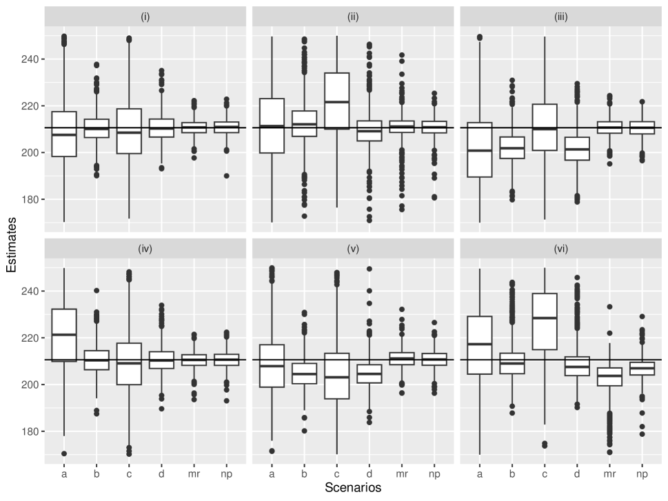
Figure 2: Simulation results for estimators of $\theta_{10}^{(10)}$ among 6 different scenarios with sample size $n=1,000$. Scenarios (i)–(vi) are described in Section 4.6. The horizontal line in each panel is the true value of $\theta_{10}^{(10)}$.

Figure 2 presents the boxplots of different estimators of $\theta_{10}^{(10)}=\mathbb{E}[Y_{1M_{0}}|U=10]$ over 1000 Monte Carlo simulations, with each panel corresponding to a specific simulation scenario. As expected, the moment-type estimators are centered around the true value if the required parametric working models are all correctly specified but generally diverge from the true value otherwise. Also, the multiply robust estimator exhibits minimum bias in Scenarios (i)–(v), confirming the quadruply robust property, but it exhibits certain bias when all of the working models are misspecied as demonstrated in scenario (vi). The nonparametric EIF-based estimator performs fairly well with minimal bias in scenarios (i)–(v), and its bias in scenario (vi) are also smaller than that of the multiply robust estimator coupled with parametric working models. For each scenario, we also investigate the 95% Wald-type confidence interval coverage rate in Table 1, where the variance is estimated by bootstrap in moment-type and multiply robust estimator and by the empirical variance of the EIF in the nonparametric method. Both $\widehat{\theta}_{10}^{(10),\text{mr}}$ and $\widehat{\theta}_{10}^{(10),\text{np}}$ present close-to-norminal coverage in scenarios (i)–(v), although their coverage rates are slightly attenuated in scenario (vi). We also evaluate estimators of $\theta_{11}^{(10)}$ and $\theta_{00}^{(10)}$ and results are qualitatively similar. The detailed additional simulation results are provided in the Supplementary Material Figures 1–2.

Table 1: Simulation results of the 95% confidence interval coverage rate among different estimators of $\theta_{10}^{(10)}$. Scenarios (i)–(vi) are described in Section 4.6.

Scenario	$\widehat{\theta}_{10}^{(10),\text{a}}$	$\widehat{\theta}_{10}^{(10),\text{b}}$	$\widehat{\theta}_{10}^{(10),\text{c}}$	$\widehat{\theta}_{10}^{(10),\text{d}}$	$\widehat{\theta}_{10}^{(10),\text{mr}}$	$\widehat{\theta}_{10}^{(10),\text{np}}$
(i)	0.951	0.924	0.910	0.930	0.929	0.969
(ii)	0.955	0.941	0.874	0.921	0.932	0.953
(iii)	0.871	0.738	0.926	0.717	0.918	0.951
(iv)	0.938	0.921	0.907	0.932	0.943	0.953
(v)	0.954	0.799	0.873	0.748	0.946	0.958
(vi)	0.953	0.919	0.657	0.870	0.732	0.812

5 Application to JOBS II randomized experiment

We reanalyze the Job Search Invervention Study (JOBS II) to illustrate the proposed methodology. JOBS II is a randomized field experiment for unemployed workers to examine the efficacy of a job training intervention to enhance individuals’ mental health and to promote high-quality reemployment (Price et al., 1992). A total of 1,801 unemployed individuals were enrolled into the study after a screening questionnaire determining their eligibility. All participants received an instructional booklet describing job-searching skills, regardless of their randomization status. Furthermore, participants in the treatment group ($Z=1$) were assigned to a job skills workshop for learning job-searching skills and enhancing inoculation against setbacks during the job-searching process. In JOBS II, the job skills workshop was only available to participants in the treatment group ($Z=1$) and participants in the control group ($Z=0$) had no access to the workshops. About 45% of the participants in the treatment group did not showed up in the job skills workshop, and this one-sided noncompliance may mask the actual benefit of the intervention. We define the actual treatment receipt as $D=1$ if the participant attend at the the job skills workshop and $D=0$ otherwise. Under our framework, we divide the study participants into two principal strata, the compliers with $D_{1}D_{0}=10$ and never takers with $D_{1}D_{0}=00$ who would always take control regardless of their assignments.

Price et al. (1992) demonstrated that the intervention is effective to reduce the unemployed workers’ depression. In this analysis, we investigate the extent to which the protective effect of the intervention on depression is transmitted through sense of mastery, a mediator identified in Price et al. (1992). Previous analyses has also examined the role of sense of mastery in disentangling the intervention-depression relationship, but some studies did not take the treatment noncompliance into consideration (for example, Imai et al., 2010a; Tchetgen Tchetgen and Shpitser, 2012) and the others who considered noncompliance invoked the exclusion restriction assumption to remove all causal pathways from the treatment assignment to the mediator and the outcome not through the actual treatment receipt (for example, Park and Kürüm, 2018, 2020). Our analysis is distinct from the previous analyses in that it addresses noncompliance without invoking exclusion restriction and hence permits the exploration of causal mechanism even among the never-takers.

The outcome $Y$ is a continuous measure of depression at 6 months after randomization based on an 11-item index of depressive symptoms, and ranges from 1 to 4 with a higher value indicating more severe depression. For the mediator, the sense of mastery was measured in a Likert scale at 6 weeks after randomization, according to the questionnaire question “how confident are you about having the skills and resources to find a suitable job in the next 4 months if you need to?” For illustration, we dichotomize this variable such that $M=0$ with answer not at all, a little or somewhat and $M=0$ with answer pretty much or a great deal. The baselines covariates ($\bm{X}$) include age, gender, race, marital status, education, assertiveness, level of economic hardship, and level of depression, which were all measured prior to randomization and considered sufficient for the ignorability assumptions for now. For the moment-type and multiply robust estimators, we used the parametric working models described in Section 4.1 for the nuisance functions. In principle, the propensity score $\pi({\bm{X}})$ is known by randomization in the JOBS II study, and therefore the working logistic regression of $\pi_{z}^{\text{par}}({\bm{X}})$ is not subject to misspecification, but we still include all baseline covariates into this working logistic regression to adjust for any chance imbalance (Zeng et al., 2021). For the nonparametric estimator, we used Super Learner with the random forest and generalized linear model libraries for estimating the nuisance functions.

Table 2 presents the estimated principal causal effect for the compliers and never takers, together with their corresponding mediation effect decompositions. It is observed all estimators closely agree with each other for all point estimates of the PNIE, PNDE, and PCE. Specifically, all estimators suggest that the JOBS II intervention exerts protective and statistically significant effect on reducing depression for compliers, and depending on the estimators in consideration, approximately 22%–26% of the principal causal effect can be explained by improvement of sense of mastery. For the never-takers, all estimators indicate a smaller but still beneficial effect of the intervention on reducing depression, but the 95% confidence interval of estimates of $\text{PCE}_{00}$ crosses zero. For example, the multiply robust estimator of $\text{PCE}_{00}$ is $-0.06$ with 95% confidence interval $(-0.16,0.03)$, which is consistent with the nonparametric estimator ($-0.05$ with 95% confidence interval $(-0.15,0.05)$) and the moment-type estimators. However, a much smaller indirect effect was detected for the never-takers, and the nonparametric estimator suggests a null indirect effect through sense of mastery ($\widehat{\text{PNIE}}_{00}^{\text{np}}=-0.001$ and 95% confidence interval $(-0.003,0.001)$). Therefore, the sense of mastery does not appear to be a mediator for intervention-depression relationship among the never-takers.

Table 2: Estimated causal effects and their 95% confidence interval in the JOBS II study.

Method	Estimand	Compliers	Never takers
a	PNIE	$-$0.030 ($-$0.062, $-$0.010)	0.014 ($-$0.068, 0.100)
	PNDE	$-$0.085 ($-$0.165, 0.006)	$-$0.080 ($-$0.171, 0.013)
	PCE	$-$0.114 ($-$0.196, $-$0.019)	$-$0.067 ($-$0.159, 0.027)
b	PNIE	$-$0.024 ($-$0.050, $-$0.006)	0.020 ($-$0.063, 0.115)
	PNDE	$-$0.088 ($-$0.169, $-$0.008)	$-$0.083 ($-$0.178, 0.017)
	PCE	$-$0.112 ($-$0.191, $-$0.023)	$-$0.064 ($-$0.161, 0.025)
c	PNIE	$-$0.026 ($-$0.064, 0.004)	0.017 ($-$0.064, 0.114)
	PNDE	$-$0.089 ($-$0.170, $-$0.011)	$-$0.083 ($-$0.180, 0.011)
	PCE	$-$0.115 ($-$0.198, $-$0.019)	$-$0.066 ($-$0.158, 0.026)
d	PNIE	$-$0.024 ($-$0.050, $-$0.006)	0.026 ($-$0.062, 0.120)
	PNDE	$-$0.087 ($-$0.170, $-$0.012)	$-$0.088 ($-$0.182, 0.008)
	PCE	$-$0.111 ($-$0.193, $-$0.024)	$-$0.062 ($-$0.160, 0.026)
mr	PNIE	$-$0.026 ($-$0.052, $-$0.008)	0.023 ($-$0.057, 0.115)
	PNDE	$-$0.089 ($-$0.169, $-$0.004)	$-$0.084 ($-$0.173, 0.013)
	PCE	$-$0.115 ($-$0.200, $-$0.026)	$-$0.061 ($-$0.157, 0.030)
np	PNIE	$-$0.021 ($-$0.044, 0.001)	$-$0.001 ($-$0.003, 0.001)
	PNDE	$-$0.076 ($-$0.162, 0.012)	$-$0.050 ($-$0.147, 0.047)
	PCE	$-$0.097 ($-$0.183, $-$0.012)	$-$0.051 ($-$0.148, 0.046)

6 A framework for sensitivity analysis

The principal ignorability (Assumption 4) and local ignorability of the mediator (Assumption 5) are two crucial assumptions for identification of the GMFs in Theorem 1. These two assumptions, however, cannot be empirically verified. Sensitivity analysis can be a useful tool to assess how the study conclusions might change under assumed violations of the ignorability conditions. In the Supplementary Material, we develop a semiparametric sensitivity analysis framework to assess the impact of violation of Assumption 4 and Assumption 5 on inference about the GMFs and mediation effects under both one-sided and two-sided noncompliance scenarios. The proposed sensitivity analysis strategy relies on the confounding function approach (Tchetgen Tchetgen and Shpitser, 2012; Ding and Lu, 2017). Once the confounding functions are developed, we further provide a generalized multiply robust estimator for the GMFs and natural mediation effects and prove its consistency and multiply robustness, assuming known confounding function. In practice, the confounding function is unknown and therefore users can specify a working sensitivity function in terms of sensitivity parameters and then report the generalized multiply robust estimator under a range of values of sensitivity parameters, in order to identify tipping points that might reverse the causal conclusions. In the Supplementary Material, we illustrate the application of the sensitivity analysis framework in the context of the JOBS II study.

7 Discussion

Our contributions to the existing literature of causal mediation methods are several-folded. First, we consider a set of new identification assumptions for studying the natural mediation effects under treatment noncompliance. The absence of exclusion restriction allows us to explore whether or not any causal effect exists among the always takers and never takers strata, and if it exists, the extent to which of such an effect works through a hypothesized mediator. Second, we derive the efficient influence function for the principal natural mediation effects and further propose quadruply robust estimators, which provide four opportunities to achieve consistency and offer stronger protection against model misspecifications. Finally, a nonparametric extension of our estimators has been developed to alleviate concerns on model misspecification and achieve efficient estimation of the principal natural mediation effects.

Our theoretical results rely on several ignorability conditions (Assumptions 2, 4, and 5). The ignorability of treatment assignment (Assumptions 2) is automatically satisfied in experimental studies where the assignment is randomized. In contrast, the principal ignorability (Assumption 4) and the local ignorability of the mediator (Assumption 5) rely critically on the the collection of pre-treatment covariates, and can still be violated even under experimental studies. Therefore, the proposed sensitivity analysis framework can be a useful tool to investigate the robustness of the estimation under departure from the assumptions of principal ignorability and local ignorability of the mediator. In the context of JOBS II randomized experiment, we illustrate the application of the proposed sensitivity analysis methods to understand the changes in mediation effect estimates under assumed departure of the ignorability assumptions, and the results are provided in Supplementary Material Figures 3–5.

While we primarly consider a single mediator under noncompliance, the proposed semparametric efficiency theory and quadruply robust estimator can be expanded to accommodate multiple mediators, such as long the lines of Zhou (2022) and Xia and Chan (2022). The extension, however, may require a careful definition of mediation effect estimands within each principal stratum, because the decomposition of the total treatment effect is no longer unique in the presence of multiple mediators (Daniel et al., 2015) and can depend on the causal ordering of the mediators. To identify those more complicated estimands, it is worth exploring the necessity of additional identification assumptions to achieve point estimation of the principal mediation effects, and investigating the properties of the multiply robust estimators. We plan to pursue such extensions in our future work.

Supplementary Material to “Identification and multiply robust estimation in mediation analysis with noncompliance”

In Section A, we provide a semiparametric sensitivity analysis framework for the principal ignorability assumption and local ignorability of the mediator assumption. In Section B, we provide the proofs for all theorems, propositions, and remarks in the main manuscript. In Section C, we present web figures referenced in the main manuscript.

A Sensitivity analysis

The principal ignorability (Assumption 4) and local ignorability of the mediator (Assumption 5) are required for the identification of the GMFs in Theorem 1. However, these two assumptions are not empirically verifiable based on the observed data. We propose sensitivity analysis strategies to assess the impact of violation of these two assumptions on inference about the GMFs. When evaluating the sensitivity to violation of one specific assumption, we shall assume all other structural assumptions hold. To fix ideas, we consider that the mediator $M$ is a multi-valued variable with finite support $M\in\{0,1,\dots,m_{\max}\}$, and the results can be generalized to a continuous mediator.

A.1 Sensitivity analysis for the principal ignorability assumption

We first focus on the scenario of two-sided noncompliance, and methods for one-sided noncompliance are discussed at end of this section. To begin with, we notice that Theorem 1 holds under a weaker version of Assumption 4 which consists of two statements:

• $\mathbb{E}_{Y_{1m}|U,\!{\bm{X}}}[Y_{1m}|10,\!{\bm{X}}]\!=\!\mathbb{E}_{Y_{1m}|U,{\bm{X}}}[Y_{1m}|11,\!{\bm{X}}]$ and $\mathbb{E}_{Y_{0m}|U,\!{\bm{X}}}[Y_{0m}|10,\!{\bm{X}}]\!=\!\mathbb{E}_{Y_{0m}|U,\!{\bm{X}}}[Y_{0m}|00,\!{\bm{X}}]$ for any $m\in\{0,\dots,m_{\max}\}$.

• $f_{M_{1}|U,{\bm{X}}}(m|10,{\bm{X}})=f_{M_{1}|U,{\bm{X}}}(m|11,{\bm{X}})$ and $f_{M_{0}|U,{\bm{X}}}(m|10,{\bm{X}})=f_{M_{0}|U,{\bm{X}}}(m|00,{\bm{X}})$ for any $m\in\{1,\dots,m_{\max}\}$.

Statement (i) requires that the expectation of $Y_{1m}$ is same between the complier and always-takers strata and the expectation of $Y_{0m}$ is same between the complier and never-takers strata, conditional on all observed covariates. Statement (ii) implicitly suggests that $f_{M_{1}|U,{\bm{X}}}(0|10,{\bm{X}})=f_{M_{1}|U,{\bm{X}}}(0|11,{\bm{X}})$ and $f_{M_{0}|U,{\bm{X}}}(0|10,{\bm{X}})=f_{M_{0}|U,{\bm{X}}}(0|00,{\bm{X}})$. Therefore, Statement (ii) requires that the distribution of $M_{1}$ are same between the complier and always-takers strata and the distribution of $M_{0}$ are same between the complier and never-takers strata, conditional on all observed covariates. Our sensitivity analysis is based on the following confounding functions measuring departure from the weaker version of principal ignorability:

$$\xi_{Y}^{(1)}(m,{\bm{x}})=\frac{\mathbb{E}_{Y_{1m}|U,{\bm{X}}}[Y_{1m}|10,{\bm{x}}]}{\mathbb{E}_{Y_{1m}|U,{\bm{X}}}[Y_{1m}|11,{\bm{x}}]},\quad\xi_{Y}^{(0)}(m,{\bm{x}})=\frac{\mathbb{E}_{Y_{0m}|U,{\bm{X}}}[Y_{0m}|10,{\bm{x}}]}{\mathbb{E}_{Y_{0m}|U,{\bm{X}}}[Y_{0m}|00,{\bm{x}}]}\quad\text{for $m=0,\dots,m_{\max}$}$$

$$\xi_{M}^{(1)}(m,{\bm{x}})=\frac{f_{M_{1}|U,{\bm{X}}}(m|10,{\bm{x}})}{f_{M_{1}|U,{\bm{X}}}(m|11,{\bm{x}})},\quad\xi_{M}^{(0)}(m,{\bm{x}})=\frac{f_{M_{0}|U,{\bm{X}}}(m|10,{\bm{x}})}{f_{M_{0}|U,{\bm{X}}}(m|00,{\bm{x}})}\quad\text{for $m=1,\dots,m_{\max}$}.$$

The first two confounding functions measure deviation of principal ignorability in the outcome variable, where $\xi_{Y}^{(1)}(m,{\bm{x}})$ measures the ratio of the mean of $Y_{1m}$ among compliers versus always-takers and $\xi_{Y}^{(0)}(m,{\bm{x}})$ measures the ratio of the mean of $Y_{0m}$ among compliers versus never-takers, conditional on ${\bm{X}}={\bm{x}}$. On the other hand, the last two confounding functions measure deviation of principal ignorability in the mediator variable, where $\xi_{M}^{(1)}(m,{\bm{x}})$ measures the relative risk of compliers against always-takers on the treated potential mediator at level $m$ and $\xi_{M}^{(0)}(m,{\bm{x}})$ measures the relative risk of compliers against never-takers on the control potential mediator at level $m$, conditional on ${\bm{X}}={\bm{x}}$. Notice that $\xi_{M}^{(1)}(m,{\bm{x}})$ and $\xi_{M}^{(0)}(m,{\bm{x}})$ are only defined for $m\geq 1$, which will determine the values of $\xi_{M}^{(1)}(0,{\bm{x}}):=\frac{f_{M_{1}|U,{\bm{X}}}(0|10,{\bm{x}})}{f_{M_{1}|U,{\bm{X}}}(0|11,{\bm{x}})}$ and $\xi_{M}^{(0)}(0,{\bm{x}}):=\frac{f_{M_{0}|U,{\bm{X}}}(0|10,{\bm{x}})}{f_{M_{0}|U,{\bm{X}}}(0|00,{\bm{x}})}$ as shown in Section B.8, where we have provided the following explicit expressions in terms of $\{\xi_{M}^{(1)}(m,{\bm{x}}),\xi_{M}^{(0)}(m,{\bm{x}})\text{ for }m=1,\dots,m_{\max}\}$:

$$\xi_{M}^{(1)}(0,{\bm{x}}) =\frac{1-\displaystyle\sum_{j=1}^{m_{\max}}\frac{\xi_{M}^{(1)}(j,{\bm{x}})p_{11}({\bm{x}})}{\xi_{M}^{(1)}(j,{\bm{x}})(p_{11}({\bm{x}})-p_{01}({\bm{x}}))+p_{01}({\bm{x}})}r_{11}(j,{\bm{x}})}{1-\displaystyle\sum_{j=1}^{m_{\max}}\frac{p_{11}({\bm{x}})}{\xi_{M}^{(1)}(j,{\bm{x}})(p_{11}({\bm{x}})-p_{01}({\bm{x}}))+p_{01}({\bm{x}})}r_{11}(j,{\bm{x}})},$$

$$\xi_{M}^{(0)}(0,{\bm{x}}) =\frac{1-\displaystyle\sum_{j=1}^{m_{\max}}\frac{\xi_{M}^{(0)}(j,{\bm{x}})p_{00}({\bm{x}})}{\xi_{M}^{(0)}(j,{\bm{x}})(p_{11}({\bm{x}})-p_{01}({\bm{x}}))+p_{10}({\bm{x}})}r_{00}(j,{\bm{x}})}{1-\displaystyle\sum_{j=1}^{m_{\max}}\frac{p_{00}({\bm{x}})}{\xi_{M}^{(0)}(j,{\bm{x}})(p_{11}({\bm{x}})-p_{01}({\bm{x}}))+p_{10}({\bm{x}})}r_{00}(j,{\bm{x}})}.$$

Theorem 1 holds if all sensitivity functions in $\xi=\Big{\{}\left(\xi_{M}^{(1)}(m,{\bm{x}}),\xi_{M}^{(0)}(m,{\bm{x}})\right)\text{ for }m=1,\dots,m_{\max}\text{ and }\left(\xi_{Y}^{(1)}(m,{\bm{x}}),\xi_{Y}^{(0)}(m,{\bm{x}})\right)\text{ for }m=0,\dots,m_{\max}\Big{\}}$ are equal to 1. The following proposition generalizes Theorem 1 to the scenario when at least one confounding function has value different from 1.

Proposition S1

Suppose that Assumptions 1, 2, 3a, 5, and 6 hold with a two-sided noncompliance scenario and known values of the confounding functions ($\xi$), we can identify $\theta_{d_{1}d_{0}}^{(zz^{\prime})}$ by

$$\theta_{d_{1}d_{0}}^{(zz^{\prime})}=\int_{{\bm{x}}}\frac{e_{d_{1}d_{0}}({\bm{x}})}{e_{d_{1}d_{0}}}\left\{\sum_{m=0}^{m_{\max}}w_{d_{1}d_{0}}^{(zz^{\prime})}(m,{\bm{x}})\mu_{zd_{z}}(m,{\bm{x}})r_{z^{\prime}d_{z^{\prime}}}(m,{\bm{x}})\right\}\text{d}\mathbb{P}_{{\bm{X}}}({\bm{x}}),$$

for any $d_{1}d_{0}\in\mathcal{U}_{\text{2-sided}}$. Here $w_{d_{1}d_{0}}^{(zz^{\prime})}(m,{\bm{x}})$ is a sensitivity weight defined in Section B.8, which depends on the confounding functions $\xi$ and the observed-data nuisance functions $p_{zd}({\bm{x}})$ and $r_{zd}(m,{\bm{x}})$. As an example,

$$w_{10}^{(10)}(m,{\bm{x}})=\begin{cases}\displaystyle\frac{\xi_{M}^{(0)}(m,{\bm{x}})p_{00}({\bm{x}})}{\xi_{M}^{(0)}(m,{\bm{x}})(p_{11}({\bm{x}})-p_{01}({\bm{x}}))+p_{10}({\bm{x}})}\displaystyle\frac{\xi_{M}^{(1)}(m,{\bm{x}})(p_{11}({\bm{x}})-p_{01}({\bm{x}}))+p_{01}({\bm{x}})}{p_{01}({\bm{x}})/\xi_{Y}^{(1)}(m,{\bm{x}})+\xi_{M}^{(1)}(m,{\bm{x}})(p_{11}({\bm{x}})-p_{01}({\bm{x}}))},&\text{if }m\geq 1,\\ \left\{\displaystyle\frac{1}{r_{00}(0,{\bm{x}})}-\displaystyle\sum_{j=1}^{m_{\max}}\frac{\xi_{M}^{(0)}(j,{\bm{x}})p_{00}({\bm{x}})r_{00}(j,{\bm{x}})/r_{00}(0,{\bm{x}})}{\xi_{M}^{(0)}(j,{\bm{x}})(p_{11}({\bm{x}})-p_{01}({\bm{x}}))+p_{10}({\bm{x}})}\right\}\displaystyle\frac{\xi_{M}^{(1)}(0,{\bm{X}})(p_{11}({\bm{x}})-p_{01}({\bm{x}}))+p_{01}({\bm{x}})}{p_{01}({\bm{x}})/\xi_{Y}^{(1)}(0,{\bm{x}})+\xi_{M}^{(1)}(0,{\bm{x}})(p_{11}({\bm{x}})-p_{01}({\bm{x}}))},&\text{if }m=0.\end{cases}$$

If $\xi$ is known, we can construct a new estimator of the GMF by carefully re-weighting each term in the original multiply robust estimator $\widehat{\theta}^{(zz^{\prime}),\text{mr}}_{d_{1}d_{0}}$ by the sensitivity weight $w_{d_{1}d_{0}}^{(zz^{\prime})}(m,{\bm{x}})$. Specifically, the new estimator, $\widehat{\theta}^{(zz^{\prime}),\text{mr}}_{d_{1}d_{0}}(\xi)$, takes the following form:

$$\widehat{\theta}^{(zz^{\prime}),\text{mr}}_{d_{1}d_{0}}(\xi)= \mathbb{P}_{n}\Big{\{}\left(\frac{\mathbb{I}(Z=z^{*})\left\{\mathbb{I}(D=d^{*})-\widehat{p}_{z^{*}d^{*}}^{\text{par}}({\bm{X}})\right\}}{\widehat{\pi}_{z^{*}}^{\text{par}}({\bm{X}})}-k\frac{(1-Z)\left\{D-\widehat{p}_{01}^{\text{par}}({\bm{X}})\right\}}{\widehat{\pi}_{0}^{\text{par}}({\bm{X}})}\right)\frac{\widehat{\eta}_{zz^{\prime}}^{w,\text{par}}({\bm{X}})}{\widehat{p}_{z^{*}d^{*}}^{\text{dr}}-k\widehat{p}_{01}^{\text{dr}}}$$

$$+\frac{\widehat{p}_{z^{*}d^{*}}^{\text{par}}({\bm{X}})-k\widehat{p}_{01}^{\text{par}}({\bm{X}})}{\widehat{p}_{z^{*}d^{*}}^{\text{dr}}-k\widehat{p}_{01}^{\text{dr}}}\frac{\mathbb{I}(D=d_{z},Z=z)}{\widehat{p}_{zd_{z}}^{\text{par}}({\bm{X}})\widehat{\pi}_{z}^{\text{par}}({\bm{X}})}\frac{\widehat{r}_{z^{\prime}d_{z^{\prime}}}^{\text{par}}(M,{\bm{X}})}{\widehat{r}_{zd_{z}}^{\text{par}}(M,{\bm{X}})}\widehat{w}_{d_{1}d_{0}}^{(zz^{\prime})}(M,{\bm{X}})\left\{Y-\widehat{\mu}_{zd_{z}}^{\text{par}}(M,{\bm{X}})\right\}$$

$$+\frac{\widehat{p}_{z^{*}d^{*}}^{\text{par}}({\bm{X}})-k\widehat{p}_{01}^{\text{par}}({\bm{X}})}{\widehat{p}_{z^{*}d^{*}}^{\text{dr}}-k\widehat{p}_{01}^{\text{dr}}}\frac{\mathbb{I}(D=d_{z^{\prime}},Z=z^{\prime})}{\widehat{p}_{z^{\prime}d_{z^{\prime}}}^{\text{par}}({\bm{X}})\widehat{\pi}_{z^{\prime}}^{\text{par}}({\bm{X}})}\left\{\widehat{w}_{d_{1}d_{0}}^{(zz^{\prime})}(M,{\bm{X}})\widehat{\mu}_{zd_{z}}^{\text{par}}(M,{\bm{X}})-\widehat{\eta}_{zz^{\prime}}^{w,\text{par}}({\bm{X}})\right\}$$

$$+\frac{\widehat{p}_{z^{*}d^{*}}^{\text{par}}({\bm{X}})-k\widehat{p}_{01}^{\text{par}}({\bm{X}})}{\widehat{p}_{z^{*}d^{*}}^{\text{dr}}-k\widehat{p}_{01}^{\text{dr}}}\widehat{\eta}_{zz^{\prime}}^{w,\text{par}}({\bm{X}})\Big{\}},$$ (s9)

where $\widehat{\eta}_{zz^{\prime}}^{w,\text{par}}({\bm{x}})=\displaystyle\sum_{m=0}^{m_{\max}}\widehat{w}_{d_{1}d_{0}}^{(zz^{\prime})}(m,{\bm{x}})\widehat{\mu}_{zd_{z}}^{\text{par}}(m,{\bm{x}})\widehat{r}_{z^{\prime}d_{z^{\prime}}}^{\text{par}}(m,{\bm{x}})$ and $\widehat{w}_{d_{1}d_{0}}^{(zz^{\prime})}(m,{\bm{x}})$ is $w_{d_{1}d_{0}}^{(zz^{\prime})}(m,{\bm{x}})$ evaluated at $\left\{\widehat{p}_{zd}^{\text{par}}({\bm{x}}),\widehat{r}_{zd}^{\text{par}}(m,{\bm{x}})\right\}$. The following proposition shows that $\widehat{\theta}^{(zz^{\prime}),\text{mr}}_{d_{1}d_{0}}(\xi)$ is a doubly robust estimator under $\mathcal{M}_{\pi+e+m}\cup\mathcal{M}_{e+m+o}$.

Proposition S2

Suppose that Assumptions 1, 2, 3a, 5, and 6 hold under two-sided noncompliance. Then, the estimator $\widehat{\theta}^{(zz^{\prime}),\text{mr}}_{d_{1}d_{0}}(\xi)$ is consistent and asymptotically normal for any $d_{1}d_{0}\in\mathcal{U}_{\text{2-sided}}$ if either $\mathcal{M}_{\pi+e+m}$ or $\mathcal{M}_{e+m+o}$ is correctly specified.

In practice, the confounding functions in $\xi$ are unknown. To conduct the sensitivity analysis, one can specify a parametric form of $\xi$ indexed by a finite dimensional parameter $\bm{\lambda}$, say $\xi_{\bm{\lambda}}$. Then, one can report $\widehat{\theta}^{(zz^{\prime}),\text{mr}}_{d_{1}d_{0}}(\xi_{\bm{\lambda}})$ and its confidence intervals over a sequence of values of $\bm{\lambda}$, which summarizes how sensitive the inference are affected under assumed departure from the principal ignorability assumption.

The above sensitivity analysis strategy can be easily extended to the scenario of one-sided noncompliance. Because there are no always-takers under one-sided noncompliance, we only need to quantify departure of the principal ignorability between the never-takers and compliers strata, that is, only $\xi_{M}^{(0)}(m,{\bm{x}})$ and $\xi_{Y}^{(0)}(m,{\bm{x}})$ are needed for sensitivity analysis. Similar to the construction of (s9), we can develop an estimator, $\widehat{\theta}^{(zz^{\prime}),\text{mr}}_{d_{1}d_{0}}(\kappa)$, based on a set of confounding functions, $\kappa=\{\xi_{M}^{(0)}(m,{\bm{x}})\text{ for $m=1,\dots,m_{\max}$},~{}\xi_{Y}^{(0)}(m,{\bm{x}})\text{ for $m=0,\dots,m_{\max}$}\}$, and this estimator is consistent to $\theta^{(zz^{\prime})}_{d_{1}d_{0}}$ under $\mathcal{M}_{\pi+e+m}\cup\mathcal{M}_{e+m+o}$ for any $d_{1}d_{0}\in\mathcal{U}_{\text{1-sided}}$. Details of $\widehat{\theta}^{(zz^{\prime}),\text{mr}}_{d_{1}d_{0}}(\kappa)$ are given in Section B.9. Analogously, one can report $\widehat{\theta}^{(zz^{\prime}),\text{mr}}_{d_{1}d_{0}}(\kappa_{\bm{\lambda}})$ over a set of choices of $\bm{\lambda}$ to quantify the values of GMF under assumed departure from principal ignorability, where $\kappa_{\bm{\lambda}}$ is user-specified parametric functions of $\kappa$.

A.2 Sensitivity analysis for the local ignorability assumption

We develop a sensitivity analysis framework to assess the extent to which the violation of Assumption 5 might affect inference of $\theta_{d_{1}d_{0}}^{(10)}$; identification of $\theta_{d_{1}d_{0}}^{(11)}$ and $\theta_{d_{1}d_{0}}^{(00)}$, however, does not depend on Assumption 5. In Section B.10, we show that the expression of $\theta_{d_{1}d_{0}}^{(10)}$ in Theorem 1 holds under a weaker version of Assumption 5 such that $\mathbb{E}_{Y_{zm}|Z,M,U,{\bm{X}}}[Y_{zm}|z,m,d_{1}d_{0},{\bm{X}}]=\mathbb{E}_{Y_{zm}|Z,M,U,{\bm{X}}}[Y_{zm}|z,0,d_{1}d_{0},{\bm{X}}]$, for all $m>0$, $z\in\{0,1\}$, $d_{1}d_{0}\in\mathcal{U}_{\text{2-sided}}$ under two-sided noncompliance, and $d_{1}d_{0}\in\mathcal{U}_{\text{1-sided}}$ under one-sided noncompliance. This weaker assumption only requires mean independence between the potential outcome and the mediator conditional the treatment assignment, principal strata, and baseline covariates. Recognizing the sufficiency of this weaker assumption, we propose the following sensitivity function to assess violations of the weaker version of Assumption 5:

$$t(z,m,d_{1}d_{0},{\bm{x}})=\frac{\mathbb{E}_{Y_{1m}|Z,M,U,{\bm{X}}}[Y_{1m}|z,m,d_{1}d_{0},{\bm{x}}]}{\mathbb{E}_{Y_{1m}|Z,M,U,{\bm{X}}}[Y_{1m}|z,0,d_{1}d_{0},{\bm{x}}]},$$

for $m\in\{0,1,\dots,m_{\max}\}$, where $t(z,0,d_{1}d_{0},{\bm{x}})\equiv 1$ by definition. If $t(z,m,d_{1}d_{0},{\bm{x}})$ differs from 1, then the identification formula of $\theta^{(10)}_{d_{1}d_{0}}$ in Theorem 1 no longer holds. The following proposition generalizes Theorem 1 to the scenario for a known $t(z,m,d_{1}d_{0},{\bm{x}})$.

Proposition S3

Suppose that Assumptions 1–4 and 6 hold. Based on the confounding function $t(z,m,d_{1}d_{0},{\bm{x}})$, we can identify $\theta^{(10)}_{d_{1}d_{0}}$ as

$$\theta^{(10)}_{d_{1}d_{0}}=\int_{{\bm{x}}}\frac{e_{d_{1}d_{0}}({\bm{x}})}{e_{d_{1}d_{0}}}\left\{\sum_{m=0}^{m_{\max}}\rho_{d_{1}d_{0}}^{(10)}(m,{\bm{x}})\mu_{1d_{1}}(m,{\bm{x}})r_{0d_{0}}(m,{\bm{x}})\right\}\text{d}\mathbb{P}_{{\bm{X}}}({\bm{x}}),$$

for any $d_{1}d_{0}\in\mathcal{U}_{\text{1-sided}}$ under one-sided noncompliance scenario and any $d_{1}d_{0}\in\mathcal{U}_{\text{2-sided}}$ under two-sided noncompliance scenario, where

$$\rho_{d_{1}d_{0}}^{(10)}(m,{\bm{x}})=\left\{\sum_{j=0}^{m_{\max}}\frac{t(1,j,d_{1}d_{0},{\bm{x}})}{t(1,m,d_{1}d_{0},{\bm{x}})}r_{1d_{1}}(j,{\bm{x}})\right\}\Big{/}\left\{\sum_{j=0}^{m_{\max}}\frac{t(0,j,d_{1}d_{0},{\bm{x}})}{t(0,m,d_{1}d_{0},{\bm{x}})}r_{0d_{0}}(j,{\bm{x}})\right\}$$

is the sensitivity weight which depends on the confounding function $t(z,m,d_{1}d_{0},{\bm{x}})$ and the observed-data nuisance function $r_{zd}(m,{\bm{x}})$.

If the sensitivity function $t=t(z,m,d_{1}d_{0},{\bm{x}})$ is known, we show in Section B.10 that a consistent estimator of $\theta^{(10)}_{d_{1}d_{0}}$ can be obtained by re-weighting each term in the multiply robust estimator by the sensitivity weight $\rho_{d_{1}d_{0}}^{(10)}(m,{\bm{X}})$, and takes the following form:

$$\widehat{\theta}^{(10),\text{mr}}_{d_{1}d_{0}}(t)= \mathbb{P}_{n}\Big{\{}\left(\frac{\mathbb{I}(Z=z^{*})\left\{\mathbb{I}(D=d^{*})-\widehat{p}_{z^{*}d^{*}}^{\text{par}}({\bm{X}})\right\}}{\widehat{\pi}_{z^{*}}^{\text{par}}({\bm{X}})}-k\frac{(1-Z)\left\{D-\widehat{p}_{01}^{\text{par}}({\bm{X}})\right\}}{\widehat{\pi}_{0}^{\text{par}}({\bm{X}})}\right)\frac{\widehat{\eta}_{10}^{\rho,\text{par}}({\bm{X}})}{\widehat{p}_{z^{*}d^{*}}^{\text{dr}}-k\widehat{p}_{01}^{\text{dr}}}$$

$$+\frac{\widehat{p}_{z^{*}d^{*}}^{\text{par}}({\bm{X}})-k\widehat{p}_{01}^{\text{par}}({\bm{X}})}{\widehat{p}_{z^{*}d^{*}}^{\text{dr}}-k\widehat{p}_{01}^{\text{dr}}}\frac{\mathbb{I}(D=d_{1},Z=1)}{\widehat{p}_{1d_{1}}^{\text{par}}({\bm{X}})\widehat{\pi}_{1}^{\text{par}}({\bm{X}})}\frac{\widehat{r}_{0d_{0}}^{\text{par}}(M,{\bm{X}})}{\widehat{r}_{1d_{1}}^{\text{par}}(M,{\bm{X}})}\widehat{\rho}_{d_{1}d_{0}}^{(10)}(M,{\bm{X}})\left\{Y-\widehat{\mu}_{1d_{1}}^{\text{par}}(M,{\bm{X}})\right\}$$

$$+\frac{\widehat{p}_{z^{*}d^{*}}^{\text{par}}({\bm{X}})-k\widehat{p}_{01}^{\text{par}}({\bm{X}})}{\widehat{p}_{z^{*}d^{*}}^{\text{dr}}-k\widehat{p}_{01}^{\text{dr}}}\frac{\mathbb{I}(D=d^{\prime},Z=z^{\prime})}{\widehat{p}_{0d_{0}}^{\text{par}}({\bm{X}})\widehat{\pi}_{0}^{\text{par}}({\bm{X}})}\left\{\widehat{\rho}_{d_{1}d_{0}}^{(10)}(M,{\bm{X}})\widehat{\mu}_{1d_{1}}^{\text{par}}(M,{\bm{X}})-\widehat{\eta}_{10}^{\rho,\text{par}}({\bm{X}})\right\}$$

$$+\frac{\widehat{p}_{z^{*}d^{*}}^{\text{par}}({\bm{X}})-k\widehat{p}_{01}^{\text{par}}({\bm{X}})}{\widehat{p}_{z^{*}d^{*}}^{\text{dr}}-k\widehat{p}_{01}^{\text{dr}}}\widehat{\eta}_{10}^{\rho,\text{par}}({\bm{X}})\Big{\}},$$

where $\widehat{\eta}_{10}^{\rho,\text{par}}({\bm{X}})=\displaystyle\sum_{m=0}^{m_{\max}}\widehat{\rho}_{d_{1}d_{0}}^{(10)}(m,{\bm{x}})\widehat{\mu}_{1d_{1}}^{\text{par}}(m,{\bm{x}})\widehat{r}_{0d_{0}}^{\text{par}}(m,{\bm{x}})$ and $\widehat{\rho}_{d_{1}d_{0}}^{(10)}(m,{\bm{x}})$ is ${\rho}_{d_{1}d_{0}}^{(10)}(m,{\bm{x}})$ evaluated at $\widehat{r}_{zd}^{\text{par}}(m,{\bm{x}})$. The following proposition shows that $\widehat{\theta}^{(10),\text{mr}}_{d_{1}d_{0}}(t)$ is a triply robust estimator under $\mathcal{M}_{\pi+e+m}\cup\mathcal{M}_{e+m+o}\cup\mathcal{M}_{\pi+m+o}$.

Proposition S4

Suppose that Assumptions 1–4 and 6 hold. Then, the estimator $\widehat{\theta}^{(10),\text{mr}}_{d_{1}d_{0}}(t)$ is consistent and asymptotically normal for any $d_{1}d_{0}\in\mathcal{U}_{\text{2-sided}}$ under two-sided noncompliance scenario and $d_{1}d_{0}\in\mathcal{U}_{\text{1-sided}}$ under one-sided noncompliance scenario, if either $\mathcal{M}_{\pi+e+m}$, $\mathcal{M}_{e+m+o}$, or $\mathcal{M}_{\pi+m+o}$ is correctly specified.

To conduct the sensitivity analysis, one can specify a parametric form of $t$ indexed by a finite dimensional parameter $\bm{\zeta}$, $t_{\bm{\zeta}}=t(z,m,d_{1}d_{0},{\bm{x}};\bm{\zeta})$. Then, one can report $\widehat{\theta}^{(zz^{\prime}),\text{mr}}_{d_{1}d_{0}}(t_{\bm{\zeta}})$ over a range of choices of $\bm{\zeta}$, which captures the sensitivity of the conclusion under departure from Assumption 5.

A.3 Illustration of the sensitivity analysis framework based on the JOBS II study

This section re-visits the JOBS II study in Section 5 to assess robustness of our conclusions to the violation of the proposed structural assumptions. The ignorability assumption of treatment assignment (Assumption 2) and strong monotonicity assumption (Assumption 3) are satisfied in JOBS II study by design, but the the principal ignorability (Assumption 4) and the local ignorability of the mediator (Assumption 5) are generally not empirically verifiable without additional data. Henceforth, we apply the proposed sensitivity analysis framework to assess robustness of the estimated principal mediation effects to the violation of Assumptions 4 and 5, separately. For the purpose of illustration, we only assess the range of the estimated principal natural mediation effects among the compliers stratum. While examining the violation of one assumption, we assume all other assumptions hold.

A.3.1 Sensitivity analysis for principal ignorability

As we discussed in Section A.1, under a one-sided noncompliance scenario with a binary mediator, the confounding functions $\kappa=\{\xi_{M}^{(0)}(1,{\bm{x}}),\xi_{Y}^{(0)}(1,{\bm{x}})\}$ can be used to measure the extent to deviation of the prinicpal ignorability assumption. Specifically, $\xi_{M}^{(0)}(1,{\bm{x}})=\frac{f_{M_{0}|U,{\bm{X}}}(1|10,{\bm{x}})}{f_{M_{0}|U,{\bm{X}}}(1|00,{\bm{x}})}$ measures the relative risk between compliers against the never-takers on the sense of mastery under the control condition and $\xi_{Y}^{(0)}(1,{\bm{x}})=\frac{E_{Y_{0m}|U,{\bm{X}}}[Y_{0m}|10,{\bm{x}}]}{E_{Y_{0m}|U,{\bm{X}}}[Y_{0m}|00,{\bm{x}}]}$ measures the ratio of the potential outcome mean (under the control condition) between compliers and never-takers. For simplicity (and this is often a practical strategy for sensitivity analysis without additional content knowledge), we assume the two confounding functions do not depend on the measured baseline covariates such that $\xi_{M}^{(0)}(1,{\bm{x}})=\lambda_{M}$ and $\xi_{Y}^{(0)}(1,{\bm{x}})=\lambda_{Y}$. Our specified parametric confounding function is thus $\kappa_{\bm{\lambda}}=\{\lambda_{M},\lambda_{Y}\}$.

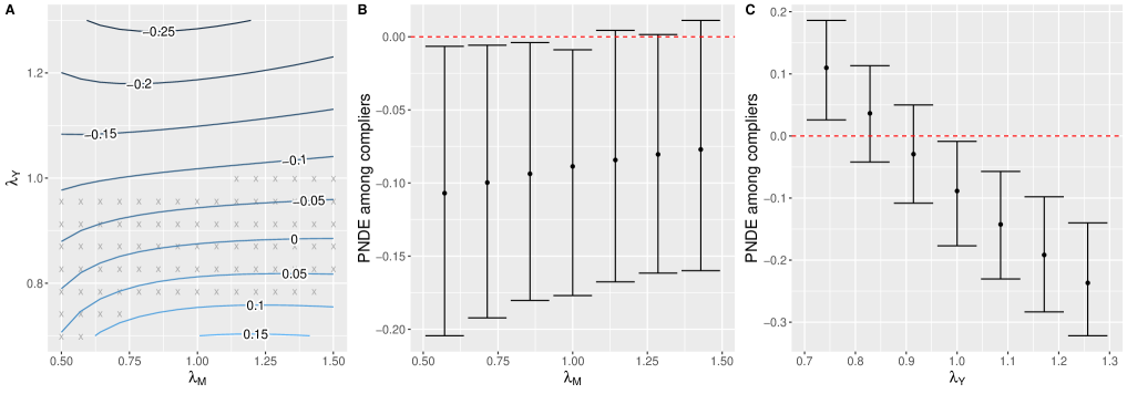
Figure S3: Sensitivity analysis of $\text{PNDE}_{10}$ to violation of the principal ignorability assumption in JOBS II study. Panel A: Contour plot of $\widehat{\text{PNDE}}_{10}=\widehat{\theta}_{10}^{(10),\text{mr}}(\xi_{\bm{\lambda}})-\widehat{\theta}_{10}^{(00),\text{mr}}(\xi_{\bm{\lambda}})$ for fixed values the sensitivity parameter $\{\lambda_{M},\lambda_{Y}\}\in[0.5,1.5]\times[0.75,1.25]$, where pixels with the mark ‘$\times$’ suggest that the corresponding 95% interval estimate covers 0. Panel B: $\widehat{\text{PNDE}}_{10}$ with its 95% interval estimate for $\lambda_{M}$ ranging from 0.5 to 1.5 while fixing $\lambda_{Y}=1$. Panel C: $\widehat{\text{PNDE}}_{10}$ with its 95% interval estimate for $\lambda_{Y}$ ranging from 0.75 to 1.25 while fixing $\lambda_{M}=1$.

Figure S3 presents the bias-corrected $\text{PNDE}_{10}$ estimate, $\widehat{\text{PNDE}}_{10}=\widehat{\theta}_{10}^{(10),\text{mr}}(\kappa_{\bm{\lambda}})-\widehat{\theta}_{10}^{(00),\text{mr}}(\kappa_{\bm{\lambda}})$, with fixed values of $\{\lambda_{M},\lambda_{Y}\}$ ranging within $[0.5,1.5]\times[0.75,1.25]$. The results suggest that ${\text{PNDE}}_{10}$ is robust to violation of the principal ignorability on the mediator variable as $\widehat{\text{PNDE}}_{10}$ has relatively small fluctuations with different values of $\lambda_{M}$. For example, $\widehat{\text{PNDE}}_{10}$ only increases from $-$0.111 (95% CI: $[-0.216,-0.008]$) to $-$0.075 (95% CI: $[-0.156,0.010]$) when varying $\lambda_{M}$ from 0.5 to 1.5 with $\lambda_{Y}$ fixed at 1 (Figure S3, Panel B). In contrast, ${\text{PNDE}}_{10}$ is more sensitive to violation of the principal ignorability on the outcome variable, because $\widehat{\text{PNDE}}_{10}$ moved toward null when $\lambda_{Y}$ decreases from $1$ and the sign of $\widehat{\text{PNDE}}_{10}$ can even be reverted to positive when $\xi_{Y}\leq 0.87$.

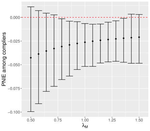
Figure S4: Sensitivity analysis of $\text{PNIE}_{10}$ to violation of the principal ignorability assumption in JOBS II study. We report $\widehat{\text{PNIE}}_{10}=\widehat{\theta}_{10}^{(11),\text{mr}}(\xi_{\bm{\lambda}})-\widehat{\theta}_{10}^{(10),\text{mr}}(\xi_{\bm{\lambda}})$ and its 95% bootstrap confidence interval with the sensitivity parameter $\lambda_{M}$ ranging from 0.5 to 1.5.

Next, we assess robustness of our conclusions on $\text{PNIE}_{10}$ under departure from principal ignorability. In the one-sided noncompliance scenario, the validity of $\widehat{\text{PNIE}}_{10}$ only depends on the principal ignorability assumption on the mediator variable (as we clarify in Section B.9, violation of principal ignorabilty on the outcome variable has no impact on $\widehat{\text{PNIE}}_{10}$). Therefore, we provide the bias-corrected $\text{PNIE}_{10}$ estimate, $\widehat{\text{PNIE}}_{10}=\widehat{\theta}_{10}^{(11),\text{mr}}(\kappa_{\bm{\lambda}})-\widehat{\theta}_{10}^{(10),\text{mr}}(\kappa_{\bm{\lambda}})$, for $\lambda_{M}$ ranging from 0.5 to 1.5 in Figure S4. The results suggest that estimates of $\text{PNIE}_{10}$ are robust against violations of principal ignorability, because $\widehat{\text{PNIE}}_{10}$ remains negative among all values of $\lambda_{M}$ considered. The estimated 95% confidence intervals, however, straddle zero when $\lambda_{M}<0.75$ or $\lambda_{M}>1.35$.

A.3.2 Sensitivity analysis for local ignorability of the mediator

We then investigate whether the conclusion about the principal mediation effects among the compliers will be subject to change if the local ignorability of the mediator is violated (while assuming all remaining assumptions hold). As indicated in Section A.2, the confounding function $t(z,1,d_{1}d_{0},{\bm{x}})=\frac{\mathbb{E}_{Y_{1m}|Z,M,U,{\bm{X}}}[Y_{1m}|z,1,d_{1}d_{0},{\bm{x}}]}{\mathbb{E}_{Y_{1m}|Z,M,U,{\bm{X}}}[Y_{1m}|z,0,d_{1}d_{0},{\bm{x}}]}$ can be used to quantify the degree of violation of the local ignorability of the mediator assumption. For simplicity, we assume $t(z,1,d_{1}d_{0},{\bm{x}})$ is constant across all levels of $z$, $d_{1}d_{0}$, and ${\bm{x}}$ and therefore focus on a one-dimensional sensitivity parameter $\zeta$ for $t(z,1,d_{1}d_{0},{\bm{x}})$; in other words, the parametric confounding function is simply taken as $t_{\bm{\zeta}}:=t(z,1,d_{1}d_{0},{\bm{x}};\zeta)=\zeta$.

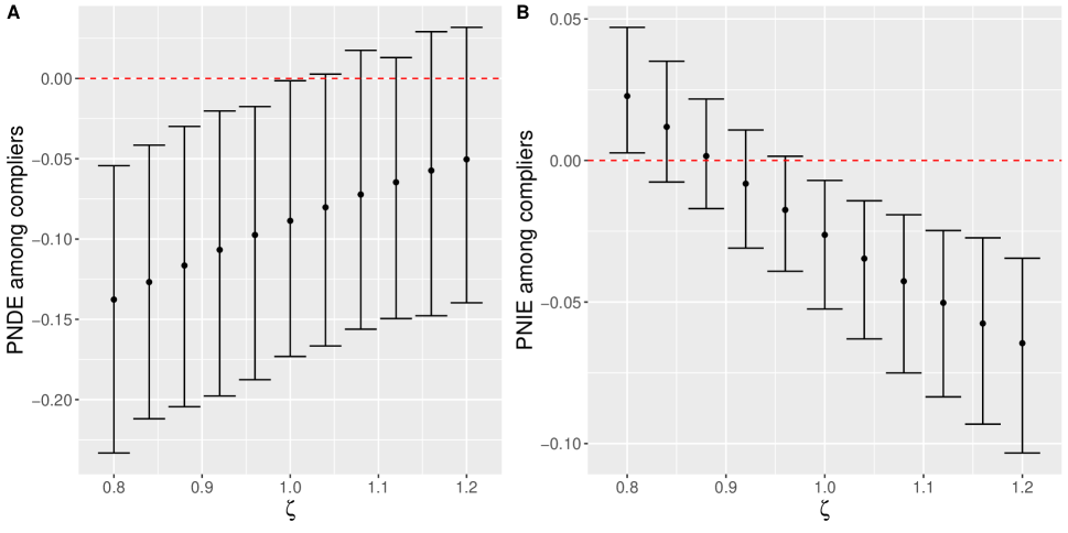
Figure S5: Sensitivity analysis of principal mediation effects among complies to violation of the local ignorability of mediator assumption in JOBS II study. Panel A: $\widehat{\text{PNDE}}_{10}=\widehat{\theta}_{10}^{(10),\text{mr}}(t_{\bm{\zeta}})-\widehat{\theta}_{10}^{(00),\text{mr}}$ and its 95% interval estimate with $\zeta$ ranging from 0.8 to 1.2. Panel B: $\widehat{\text{PNIE}}_{10}=\widehat{\theta}_{10}^{(11),\text{mr}}-\widehat{\theta}_{10}^{(10),\text{mr}}(t_{\bm{\zeta}})$ and its 95% interval estimate with $\zeta$ ranging from 0.8 to 1.2.

Figure S5 presents the bias-corrected estimates of $\text{PNDE}_{10}$, by $\widehat{\text{PNDE}}_{10}=\widehat{\theta}_{10}^{(10),\text{mr}}(t_{\bm{\zeta}})-\widehat{\theta}_{10}^{(00),\text{mr}}$, and the bias-corrected estimates of $\text{PNIE}_{10}$, by $\widehat{\text{PNIE}}_{10}=\widehat{\theta}_{10}^{(11),\text{mr}}-\widehat{\theta}_{10}^{(10),\text{mr}}(t_{\bm{\zeta}})$, with $\zeta$ varying from 0.8 to 1.2. We observe that $\widehat{\text{PNDE}}_{10}$ and $\widehat{\text{PNIE}}_{10}$ move towards null with a larger and smaller value of $\zeta$, respectively. Specifically, we observe that $\widehat{\text{PNDE}}_{10}$ remains negative under all assumed values of $\zeta$, but the point estimate increases from $-$0.137 (95% CI: $[-0.233-0.0542]$) to $-$0.050 (95% CI: $[-0.139,0.031]$) when $\zeta$ moves from 0.8 to 1.2. On the other hand, $\widehat{\text{PNIE}}_{10}$ decreases from 0.022 (95% CI: $[0.003,0.047]$) to $-$0.065 (95% CI: $[-0.103,-0.034]$), when $\zeta$ increases from 0.8 and 1.2, suggesting that $\widehat{\text{PNIE}}_{10}$ is relatively more sensitive to violation of Assumption 5.

B Proofs and technical details

B.1 The nonparametric identification result (Theorem 1)

Lemma S1

Let $X$ and $V$ be two random variables with densities $f_{X}(x)$ and $f_{V}(v)$. Then, we have that $\mathbb{E}[h(X)|V=v]=\int_{v}\frac{f_{V|X}(v|x)}{f_{V}(v)}h(x)\text{d}\mathbb{P}_{X}(x)$.

Proof.

The proof is straightforward and omitted. $\square$

Lemma S2

Let $X$, $V$, and $G$ be three random variables, then

$$X\perp\!\!\!\perp\{V,G\}\Longleftrightarrow X\perp\!\!\!\perp V|G\text{ and }X\perp\!\!\!\perp G|V.$$

Proof.

First suppose that $X\perp\!\!\!\perp\{V,G\}$ holds, then we have that for any $x$, $v$, $g$,

$$f_{X,V|G}(c,v|g)=\frac{f_{X,V,G}(x,v,g)}{f_{G}(g)}=\frac{f_{X}(x)f_{V,G}(v,g)}{f_{G}(g)}=f_{X}(x)f_{V|G}(v|g)=f_{X|G}(x|g)f_{V|G}(v|g),$$

which implies that $X\perp\!\!\!\perp V|G$. Using the same argument but switching the role of $G$ and $V$, we can show $X\perp\!\!\!\perp G|V$ under $X\perp\!\!\!\perp\{V,G\}$. Next suppose $X\perp\!\!\!\perp V|G\text{ and }X\perp\!\!\!\perp G|V$, which imply that

$$f_{X}(x) =\int_{g}f_{X|G}(x|g)\text{d}\mathbb{P}_{G}(g)=\int_{g}f_{X|G,V}(x|g,v)\text{d}\mathbb{P}_{G}(g)=\int_{g}f_{X|V}(x|v)\text{d}\mathbb{P}_{G}(g)$$

$$=f_{X|V}(x|v),$$ (s10)

for any $x$ and $v$. Therefore, we can show that for any $x,v,g$:

$$f_{X,V,G}(x,v,g) =f_{X|V,G}(x|v,g)f_{V,G}(v,g)=f_{X|V}(x|v)f_{V,G}(v,g)=f_{X}(x)f_{V,G}(v,g),$$

where the last equality follows from equation (s10). This concludes $X\perp\!\!\!\perp\{V,G\}$. $\square$

Lemma S3

The principal ignorability assumption (Assumption 4) indicates that $\{M_{zd},Y_{z^{\prime}dm^{\prime}}\}\perp\!\!\!\perp\{D_{1},D_{0}\}|{\bm{X}}$ for any $z$, $z^{\prime}$, $d$, and $m^{\prime}$, which further implies

$$M_{zd}\perp\!\!\!\perp D_{1-z}|D_{z},{\bm{X}}\text{ and }Y_{z^{\prime}dm^{\prime}}\perp\!\!\!\perp D_{1-z^{\prime}}|M_{zd},D_{z^{\prime}},{\bm{X}}.$$

Proof.

Observing $U=\{D_{1},D_{0}\}$, we can see that Assumption 4 is equivalent to $\{M_{zd},Y_{z^{\prime}dm^{\prime}}\}\perp\!\!\!\perp\{D_{1},D_{0}\}|{\bm{X}}$, which implies

$$M_{zd}\perp\!\!\!\perp\{D_{1},D_{0}\}|{\bm{X}}\text{ and }\{Y_{z^{\prime}dm^{\prime}},M_{zd}\}\perp\!\!\!\perp\{D_{1},D_{0}\}|{\bm{X}}.$$

In addition, since $\{D_{1},D_{0}\}$ is equivalent to $\{D_{z},D_{1-z}\}$ or $\{D_{z^{\prime}},D_{1-z^{\prime}}\}$, one can verify that

$$M_{zd}\perp\!\!\!\perp\{D_{z},D_{1-z}\}|{\bm{X}}\text{ and }\{Y_{z^{\prime}dm^{\prime}},M_{zd}\}\perp\!\!\!\perp\{D_{z^{\prime}},D_{1-z^{\prime}}\}|{\bm{X}}$$

hold. Therefore, $M_{zd}\perp\!\!\!\perp D_{1-z}|D_{z},{\bm{X}}$ follows from Lemma S2, with $X=M_{zd}$, $V=D_{1-z}$, and $G=D_{z}$, conditional on ${\bm{X}}$. Similarly, one can show $\{Y_{z^{\prime}dm^{\prime}},M_{zd}\}\perp\!\!\!\perp D_{1-z^{\prime}}|D_{z^{\prime}},{\bm{X}}$ by applying Lemma S2, with $X=\{Y_{z^{\prime}dm^{\prime}},M_{zd}\}$, $V=D_{1-z^{\prime}}$, and $G=D_{z^{\prime}}$, conditional on ${\bm{X}}$. Finally, $Y_{z^{\prime}dm^{\prime}}\perp\!\!\!\perp D_{1-z^{\prime}}|M_{zd},D_{z^{\prime}},{\bm{X}}$ follows by applying Lemma S2 again, with $X=D_{1-z^{\prime}}$, $V=Y_{z^{\prime}dm^{\prime}}$, and $G=M_{zd}$, conditional on ${\bm{X}}$. $\square$

Lemma S4

Let $V$ and $G$ be two binary random variables satisfying $V\geq G$ and $X$ be any random variable, then we have

$$X\perp\!\!\!\perp\{V,G\}\Longleftrightarrow X\perp\!\!\!\perp V\text{ and }X\perp\!\!\!\perp G.$$

Proof.

This follows from Lemma S1 in Forastiere et al. (2018). $\square$

Lemma S5

Under monotonicity (either Assumption 3a or 3b), Assumption 2 implies that $\{U,M_{z^{\prime}d^{\prime}},Y_{z^{*}d^{*}m^{*}}\}\perp\!\!\!\perp Z|{\bm{X}},$ for any $z^{\prime}$, $z^{*}$, $d^{\prime}$, $d^{*}$, $m^{*}$.

Proof.

Assumption 2 suggests that

$$\{D_{1},M_{z^{\prime}d^{\prime}},Y_{z^{*}d^{\prime}m^{*}}\}\perp\!\!\!\perp Z|{\bm{X}}\text{ and }\{D_{0},M_{z^{\prime}d^{\prime}},Y_{z^{*}d^{\prime}m^{*}}\}\perp\!\!\!\perp Z|{\bm{X}},$$

for any $z^{\prime}$, $z^{*}$, $d^{\prime}$, and $m^{*}$. Therefore,

$$D_{1}\perp\!\!\!\perp Z|M_{z^{\prime}d^{\prime}},Y_{z^{*}d^{\prime}m^{*}},{\bm{X}}\text{ and }D_{0}\perp\!\!\!\perp Z|{\bm{X}},M_{z^{\prime}d^{\prime}},Y_{z^{*}d^{\prime}m^{*}}$$ (s11)

follow from Lemma S2. Moreover, (s11) further implies

$$\{D_{1},D_{0}\}\perp\!\!\!\perp Z|M_{z^{\prime}d^{\prime}},Y_{z^{*}d^{\prime}m^{*}},{\bm{X}}\Longleftrightarrow U\perp\!\!\!\perp Z|M_{z^{\prime}d^{\prime}},Y_{z^{*}d^{\prime}m^{*}},{\bm{X}},$$ (s12)

by applying Lemma S4, with $V=D_{1}$, $G=D_{0}$, and $X=Z$, conditional on $\{M_{z^{\prime}d^{\prime}},Y_{z^{*}d^{\prime}m^{*}},{\bm{X}}\}$. Therefore, we have that

$$f(Z,U,M_{z^{\prime}d^{\prime}},Y_{z^{*}d^{\prime}m^{*}}|{\bm{X}})$$

$$= f(Z,U|M_{z^{\prime}d^{\prime}},Y_{z^{*}d^{\prime}m^{*}},{\bm{X}})f(M_{z^{\prime}d^{\prime}},Y_{z^{*}d^{\prime}m^{*}}|{\bm{X}})$$

$$= f(Z|M_{z^{\prime}d^{\prime}},Y_{z^{*}d^{\prime}m^{*}},{\bm{X}})f(U|M_{z^{\prime}d^{\prime}},Y_{z^{*}d^{\prime}m^{*}},{\bm{X}})f(M_{z^{\prime}d^{\prime}},Y_{z^{*}d^{\prime}m^{*}}|{\bm{X}})\quad(\text{by \eqref{eq:lemma5_2}})$$

$$= f(Z|{\bm{X}})f(U|M_{z^{\prime}d^{\prime}},Y_{z^{*}d^{\prime}m^{*}},{\bm{X}})f(M_{z^{\prime}d^{\prime}},Y_{z^{*}d^{\prime}m^{*}}|{\bm{X}})\quad(\text{by Assumption 2})$$

$$= f(Z|{\bm{X}})f(U,M_{z^{\prime}d^{\prime}},Y_{z^{*}d^{\prime}m^{*}}|{\bm{X}}).$$

This equation then shows that $\{U,M_{z^{\prime}d^{\prime}},Y_{z^{*}d^{\prime}m^{*}}\}\perp\!\!\!\perp Z|{\bm{X}}$ for any $z^{\prime}$, $z^{*}$, $d^{\prime}$, and $m^{*}$. $\square$

Proof of Theorem 1. Define $d_{z}=\mathbb{I}(z=1)d_{1}+\mathbb{I}(z=0)d_{0}$ such that $d_{z}=d_{1}$ and $d_{0}$ if $z$ in $\theta_{d_{1}d_{0}}^{(zz^{\prime})}$ is 1 and 0, respectively. Similarly, define $d_{z^{\prime}}=\mathbb{I}(z^{\prime}=1)d_{1}+\mathbb{I}(z^{\prime}=0)d_{0}$, $d_{1-z}=\mathbb{I}(z=0)d_{1}+\mathbb{I}(z=1)d_{0}$, and $d_{1-z^{\prime}}=\mathbb{I}(z^{\prime}=0)d_{1}+\mathbb{I}(z^{\prime}=1)d_{0}$. By the definition of $\theta_{d_{1}d_{0}}^{(zz^{\prime})}$, we have that

$$\theta_{d_{1}d_{0}}^{(zz^{\prime})} =\mathbb{E}[Y_{zM_{z^{\prime}}}|U=d_{1}d_{0}]$$

$$=\mathbb{E}\left[\mathbb{E}[Y_{zM_{z^{\prime}}}|U=d_{1}d_{0},{\bm{X}}]\Big{|}U=d_{1}d_{0}\right]\quad\text{(by law of iterated expectations)}$$

$$=\mathbb{E}\left[\mathbb{E}[Y_{zM_{z^{\prime}}}|Z=z,U=d_{1}d_{0},{\bm{X}}]\Big{|}U=d_{1}d_{0}\right]\quad\text{(by Lemma \ref{lemma:randomization2})}$$

$$=\mathbb{E}\left[\int_{m}\mathbb{E}[Y_{zm}|Z=z,M_{z^{\prime}}=m,U=d_{1}d_{0},{\bm{X}}]\text{d}\mathbb{P}_{M_{z^{\prime}}|Z,U,{\bm{X}}}(m|z,d_{1}d_{0},{\bm{X}})\Big{|}U=d_{1}d_{0}\right]$$

$$=\mathbb{E}\left[\int_{m}\mathbb{E}[Y_{zm}|Z=z,M_{z}=m,U=d_{1}d_{0},{\bm{X}}]\text{d}\mathbb{P}_{M_{z^{\prime}}|Z,U,{\bm{X}}}(m|z,d_{1}d_{0},{\bm{X}})\Big{|}U=d_{1}d_{0}\right]$$

(by Assumption 5)

$$=\mathbb{E}\left[\int_{m}\mathbb{E}[Y_{zm}|M_{z}=m,U=d_{1}d_{0},{\bm{X}}]\text{d}\mathbb{P}_{M_{z^{\prime}}|U,{\bm{X}}}(m|d_{1}d_{0},{\bm{X}})\Big{|}U=d_{1}d_{0}\right]\quad\text{(by Lemma \ref{lemma:randomization2})}$$

$$=\mathbb{E}\left[\int_{m}\mathbb{E}[Y_{zD_{z}m}|M_{zD_{z}}=m,U=d_{1}d_{0},{\bm{X}}]\text{d}\mathbb{P}_{M_{z^{\prime}D_{z^{\prime}}}|U,{\bm{X}}}(m|d_{1}d_{0},{\bm{X}})\Big{|}U=d_{1}d_{0}\right]$$

(by composition of potential values)

$$=\mathbb{E}\left[\int_{m}\mathbb{E}[Y_{zD_{z}m}|D_{z}\!=\!d_{z},D_{1\!-\!z}\!=\!d_{1-z},M_{zD_{z}}\!=\!m,{\bm{X}}]\text{d}\mathbb{P}_{M_{z^{\prime}D_{z^{\prime}}}|D_{z^{\prime}},D_{1-z^{\prime}},{\bm{X}}}(m|d_{z^{\prime}},d_{1-z^{\prime}},{\bm{X}})\Big{|}U\!=\!d_{1}d_{0}\right]$$

$$=\mathbb{E}\left[\int_{m}\mathbb{E}[Y_{zD_{z}m}|D_{z}\!=\!d_{z},M_{zD_{z}}\!=\!m,{\bm{X}}]\text{d}\mathbb{P}_{M_{z^{\prime}D_{z^{\prime}}}|D_{z^{\prime}},{\bm{X}}}(m|d_{z^{\prime}},{\bm{X}})\Big{|}U\!=\!d_{1}d_{0}\right]\quad\text{(by Lemma \ref{lemma:pi_v2})}$$

$$=\mathbb{E}\left[\int_{m}\mathbb{E}[Y_{zD_{z}m}|Z=z,D_{z}\!=\!d_{z},M_{zD_{z}}\!=\!m,{\bm{X}}]\text{d}\mathbb{P}_{M_{z^{\prime}D_{z^{\prime}}}|Z,D_{z^{\prime}},{\bm{X}}}(m|z^{\prime},d_{z^{\prime}},{\bm{X}})\Big{|}U\!=\!d_{1}d_{0}\right]$$

$$=\mathbb{E}\left[\int_{m}\mathbb{E}[Y|Z=z,D=d_{z},M=m,{\bm{X}}]\text{d}\mathbb{P}_{M|Z,D,{\bm{X}}}(m|z^{\prime},d_{z^{\prime}},{\bm{X}})\Big{|}U=d_{1}d_{0}\right]\quad\text{(by Assumption 1)}$$

$$=\int_{{\bm{x}}}\frac{f_{U|{\bm{X}}}(d_{1}d_{0}|{\bm{x}})}{f_{U}(d_{1}d_{0})}\int_{m}\mathbb{E}_{Y|Z,D,M,{\bm{X}}}[Y|z,d_{z},m,{\bm{X}}]\text{d}\mathbb{P}_{M|Z,D,{\bm{X}}}(m|z^{\prime},d_{z^{\prime}},{\bm{X}})\text{d}\mathbb{P}_{{\bm{X}}}({\bm{x}})\quad\text{(by Lemma \ref{lemma:expectation})}$$

$$=\int_{{\bm{x}}}\frac{e_{d_{1}d_{0}}({\bm{x}})}{e_{d_{1}d_{0}}}\int_{m}\mathbb{E}_{Y|Z,D,M,{\bm{X}}}[Y|z,d_{z},m,{\bm{X}}]\text{d}\mathbb{P}_{M|Z,D,{\bm{X}}}(m|z^{\prime},d_{z^{\prime}},{\bm{X}})\text{d}\mathbb{P}_{{\bm{X}}}({\bm{x}}),$$

where $e_{d_{1}d_{0}}({\bm{x}})=p_{z^{*}d^{*}}({\bm{x}})-kp_{01}({\bm{x}})$ and $e_{d_{1}d_{0}}=p_{z^{*}d^{*}}-kp_{01}$ are identified in equation (3) of the main manuscript under the monotonicity assumption (either Assumption 3a or 3b). This completes the proof. $\square$

B.2 Connections to existing literature (Remarks 1 and 2)

We compare the identification assumptions used in the current article to the identification assumptions in Zhou (2022) and VanderWeele et al. (2014). Specifically, Zhou (2022) considers identification of path-specific effects in the presence of multiple causally-ordered mediators and VanderWeele et al. (2014) considers identification of mediation effects in the presence of an exposure-induced confounder.

We focus on a comparable scenario with two intermediate variables, a binary variable $D$ and a binary/continuous variable $M$, both of which sit in the causal pathway between the treatment assignment $Z$ and an outcome $Y$, and we further assume the monotonicity assumption of $Z$ on $D$ (either Assumption 3a or Assumption 3b) holds. These two intermediate variables, $(D,M)$, have different names in these three papers; they are referred to as the actual treatment receipt status and the mediator in the the current paper, as the first mediator and the second mediator in Zhou (2022), and as the treatment-induced confounder and the mediator in VanderWeele et al. (2014). All three papers consider the consistency assumption (Assumption 1) and slightly different versions of positivity assumption. To offer a common ground for comparison of key identification assumptions, throughout the comparison, we always assume the consistency (Assumption 1) and the positivity (Assumption 6) hold. Besides the consistency and positivity assumptions, VanderWeele et al. (2014) consider the monotonicity assumption (Assumption 3a) and the following NPSEM-IE holds:

Assumption S1 (NPSEM-IE in VanderWeele et al., 2014)

Suppose the following nonparametric structural equation models with independent errors hold:

• ${\bm{X}}=g_{\bm{X}}(\epsilon_{\bm{X}})$,

• $Z=g_{Z}({\bm{X}},\epsilon_{Z})$,

• $D=g_{D}(Z,{\bm{X}},\epsilon_{D})$,

• $M=g_{M}(Z,D,{\bm{X}},\epsilon_{M})$,

• $Y=g_{Y}(Z,D,M,{\bm{X}},\epsilon_{Y})$,

where $\{g_{\bm{X}},g_{Z},g_{D},g_{M},g_{Y}\}$ are nonparametric functions and the errors $\{\epsilon_{\bm{X}},\epsilon_{Z},\epsilon_{D},\epsilon_{M},\epsilon_{Y}\}$ are mutually independent.

Besides the consistency and positivity assumptions, Zhou (2022) consider the following generalized sequential ignorability assumptions:

Assumption S2 (Assumption 2 in Zhou, 2022)

Suppose the following set of ignorability assumptions hold:

• $\{D_{z},M_{z^{\prime}d^{\prime}},Y_{z^{*}d^{\prime}m^{*}}\}\perp\!\!\!\perp Z|{\bm{X}}$ for any $z$, $z^{\prime}$, $d^{\prime}$, $z^{*}$, $m^{*}$,

• $\{M_{zd},Y_{z^{\prime}dm^{\prime}}\}\perp\!\!\!\perp D_{z^{*}}|Z,{\bm{X}}$ for any $z$, $z^{\prime}$, $z^{*}$, $d$, $m^{\prime}$,

• $M_{zd}\perp\!\!\!\perp Y_{z^{\prime}d^{\prime}m^{\prime}}|Z,D,{\bm{X}}$ for any $z$, $z^{\prime}$, $d$, $d^{\prime}$, $m^{\prime}$.

Besides the consistency and positivity assumptions, the current work considers Assumptions 2, 4, 5. To facilitate exposition, we restate these three assumptions:

Assumption S3 (Assumptions 2, 4 and 5 in current work)

Suppose the following ignorability assumptions hold:

• $\{D_{z},M_{z^{\prime}d^{\prime}},Y_{z^{*}d^{\prime}m^{*}}\}\perp\!\!\!\perp Z|{\bm{X}}$ for any $z$, $z^{\prime}$, $z^{*}$, $d^{\prime}$, and $m^{*}$,

• $\{M_{zd},Y_{z^{\prime}dm^{\prime}}\}\perp\!\!\!\perp U|{\bm{X}}$ for any $z$, $z^{\prime}$, $d$, and $m^{\prime}$,

• $M_{zd}\perp\!\!\!\perp Y_{z^{\prime}d^{\prime}m^{\prime}}|Z,U,{\bm{X}}$ for any $z$, $z^{\prime}$, $d$, $d^{\prime}$, $m^{\prime}$.

The following two lemmas are useful to prove Remarks 1 and 2 in the paper.

Lemma S6

Suppose that Assumptions 1 and 3 hold. Then, if Assumption S1 holds, Assumption S2 also holds, but not vice versa.

Proof.

First suppose that Assumption S1 holds. According to Assumption S1 and by the consistency (Assumption 1) and composition of potential values, we have

$$Z =g_{Z}({\bm{X}},\epsilon_{Z})$$

$$D_{z} =g_{D}(z,{\bm{X}},\epsilon_{D})$$ (s13)

$$M_{z^{\prime}d^{\prime}} =g_{M}(z^{\prime},d^{\prime},{\bm{X}},\epsilon_{M})$$ (s14)

$$Y_{z^{*}d^{\prime}m^{*}} =g_{Y}(z^{*},d^{\prime},m^{*},{\bm{X}},\epsilon_{Y})$$ (s15)

for any $z$, $z^{\prime}$, $z^{*}$, $d^{\prime}$, and $m^{*}$, which indicates that $\{D_{z},M_{z^{\prime}d^{\prime}},Y_{z^{*}d^{\prime}m^{*}}\}\perp\!\!\!\perp Z|{\bm{X}}$ because $\{\epsilon_{Z},\epsilon_{D},\epsilon_{M},\epsilon_{Y}\}$ are mutually independent. Therefore, Assumption S2(i) holds. Moreover, equations (s13), (s14), and (s15) suggest that

$$\{M_{zd},Y_{z^{\prime}dm^{\prime}}\}\perp\!\!\!\perp D_{z^{*}}|{\bm{X}},$$ (s16)

for any $z$, $z^{\prime}$, $z^{*}$, $d$, $m^{\prime}$. This implies

$$f(M_{zd},Y_{z^{\prime}dm^{\prime}},D_{z^{*}}|{\bm{X}})=f(M_{zd},Y_{z^{\prime}dm^{\prime}}|{\bm{X}})f(D_{z^{*}}|{\bm{X}}),$$

which, together with Assumption S2(i), implies that

$$f(M_{zd},Y_{z^{\prime}dm^{\prime}},D_{z^{*}}|Z,{\bm{X}})=f(M_{zd},Y_{z^{\prime}dm^{\prime}}|Z,{\bm{X}})f(D_{z^{*}}|Z,{\bm{X}}).$$

Therefore, Assumption S2(ii) hold. Similarly, equations (s14) and (s15) suggest that $M_{zd}\perp\!\!\!\perp Y_{z^{\prime}d^{\prime}m^{\prime}}|{\bm{X}}$ for any $z$, $z^{\prime}$, $d$, $d^{\prime}$, $m^{\prime}$, which indicates

$$f(M_{zd},Y_{z^{\prime}d^{\prime}m^{\prime}}|{\bm{X}})=f(M_{zd}|{\bm{X}})f(Y_{z^{\prime}d^{\prime}m^{\prime}}|{\bm{X}}).$$

This, coupled with (s16), suggests that

$$f(M_{zd},Y_{z^{\prime}d^{\prime}m^{\prime}}|D_{z^{*}},{\bm{X}})=f(M_{zd}|D_{z^{*}},{\bm{X}})f(Y_{z^{\prime}d^{\prime}m^{\prime}}|D_{z^{*}},{\bm{X}}),$$

for any $z^{*}$, which further implies

$$f(M_{zd},Y_{z^{\prime}d^{\prime}m^{\prime}}|Z=z^{*},D_{z^{*}},{\bm{X}})=f(M_{zd}|Z=z^{*},D_{z^{*}},{\bm{X}})f(M_{zd}|Z=z^{*},D_{z^{*}},{\bm{X}})$$

as a consequence of Assumption S2(i). Because $D_{z^{*}}=D$ if $Z=z^{*}$, we conclude that Assumption S2(iii) holds. Now we complete the proof that Assumption S2 also holds if Assumption S1 is valid. However, Assumption S1 may not hold under Assumption S2; that is, Assumption S1 is stronger than Assumption S2. For example, Assumption S2 does not require $\{M_{zd},M_{z^{\prime}d^{\prime}}\}\perp\!\!\!\perp Z|{\bm{X}}$ for $zd\neq z^{\prime}d^{\prime}$, but Assumption S1 implicitly require this by the following set of nonparamteric structural equations:

$$Z =g_{Z}({\bm{X}},\epsilon_{Z}),$$

$$M_{zd} =g_{M}(z,d,{\bm{X}},\epsilon_{M}),$$

$$M_{z^{\prime}d^{\prime}} =g_{M}(z^{\prime},d^{\prime},{\bm{X}},\epsilon_{M}).$$

$\square$

Lemma S7

Suppose that Assumptions 1 and 3 hold. Then, Assumption S2 is equivalent to Assumption S3.

Proof.

Assumption S2(i) is same to Assumption S3(i) by direct comparison. Next we show Assumption S2(ii) is equivalent to Assumption S3(ii) under Assumption S2(i) (or equivalently Assumption S3(i)). Specifically, under Assumption S2(i), Assumption S2(ii) suggests that

$$f(M_{zd},Y_{z^{\prime}dm^{\prime}},D_{z^{*}}|{\bm{X}}) =f(M_{zd},Y_{z^{\prime}dm^{\prime}},D_{z^{*}}|Z,{\bm{X}})$$

$$=f(M_{zd},Y_{z^{\prime}dm^{\prime}}|Z,{\bm{X}})f(D_{z^{*}}|Z,{\bm{X}})$$

$$=f(M_{zd},Y_{z^{\prime}dm^{\prime}}|{\bm{X}})f(D_{z^{*}}|{\bm{X}}).$$

That is, $\{M_{zd},Y_{z^{\prime}dm^{\prime}}\}\perp\!\!\!\perp D_{z^{*}}|{\bm{X}}$ for any $z$, $z^{\prime}$, $z^{*}$, $d$, and $m^{\prime}$, which further implies that

$$\{M_{zd},Y_{z^{\prime}dm^{\prime}}\}\perp\!\!\!\perp D_{1}|{\bm{X}}\text{ and }\{M_{zd},Y_{z^{\prime}dm^{\prime}}\}\perp\!\!\!\perp D_{0}|{\bm{X}}.$$

Applying Lemma S4 to the previous equation and noting that $D_{1}\geq D_{0}$ by monotonicity, we obtain $\{M_{zd},Y_{z^{\prime}dm^{\prime}}\}\perp\!\!\!\perp U|{\bm{X}}$; i.e., Assumption S3(ii) holds under Assumption S2(i)–(ii). On the other hand, suppose that Assumption S3(ii) hold, then we can obtain that $\{M_{zd},Y_{z^{\prime}dm^{\prime}}\}\perp\!\!\!\perp D_{1}|{\bm{X}}\text{ and }\{M_{zd},Y_{z^{\prime}dm^{\prime}}\}\perp\!\!\!\perp D_{0}|{\bm{X}}$, by Lemma S4. This suggests that

$$\{M_{zd},Y_{z^{\prime}dm^{\prime}}\}\perp\!\!\!\perp D_{z^{*}}|{\bm{X}},$$

for any $z$, $z^{\prime}$, $z^{*}$, $d$, and $m^{\prime}$. Then applying Assumption S2(i), we have

$$f(M_{zd},Y_{z^{\prime}dm^{\prime}},D_{z^{*}}|Z,{\bm{X}})= f(M_{zd},Y_{z^{\prime}dm^{\prime}},D_{z^{*}}|{\bm{X}})=f(M_{zd},Y_{z^{\prime}dm^{\prime}}|{\bm{X}})f(D_{z^{*}}|{\bm{X}}),$$

$$= f(M_{zd},Y_{z^{\prime}dm^{\prime}}|Z,{\bm{X}})f(D_{z^{*}}|Z,{\bm{X}})$$

thus Assumption S2(ii) also holds under Assumption S3(i)–(ii). Therefore, we have verified that S2(i)–(ii) are equivalent to Assumption S3(i)–(ii).

Next, we show that Assumption S2(iii) is equivalent to Assumption S3(iii) under Assumption S2(i)–(ii) (or equivalently, Assumption S3(i)–(ii)). When the monotonicity assumption (Assumption 3) holds, the following statements are equivalent under Assumption S2(i)–(ii) and Assumption S3(i)–(ii):

Assumption S3(iii)

$$\Longleftrightarrow f(M_{zd},Y_{z^{\prime}d^{\prime}m^{\prime}}|Z,U,{\bm{X}})=f(Y_{z^{\prime}d^{\prime}m^{\prime}}|Z,U,{\bm{X}})f(M_{zd}|Z,U,{\bm{X}})$$

(by Lemma S5)

$$\Longleftrightarrow f(M_{zd},Y_{z^{\prime}d^{\prime}m^{\prime}}|U,{\bm{X}})=f(Y_{z^{\prime}d^{\prime}m^{\prime}}|U,{\bm{X}})f(M_{zd}|U,{\bm{X}})$$

(by Assumption S3(ii))

$$\Longleftrightarrow f(M_{zd},Y_{z^{\prime}d^{\prime}m^{\prime}}|{\bm{X}})=f(Y_{z^{\prime}d^{\prime}m^{\prime}}|{\bm{X}})f(M_{zd}|{\bm{X}})$$

(by Assumption S3(i) or Assumption S2(i))

$$\Longleftrightarrow f(M_{zd},Y_{z^{\prime}d^{\prime}m^{\prime}}|Z,{\bm{X}})=f(Y_{z^{\prime}d^{\prime}m^{\prime}}|Z,{\bm{X}})f(M_{zd}|Z,{\bm{X}})$$

(by Assumption S2(ii))

$$\Longleftrightarrow f(M_{zd},Y_{z^{\prime}d^{\prime}m^{\prime}}|Z,D_{z^{*}},{\bm{X}})=f(Y_{z^{\prime}d^{\prime}m^{\prime}}|Z,D_{z^{*}},{\bm{X}})f(M_{zd}|Z,D_{z^{*}},{\bm{X}})$$

$$\Longleftrightarrow f(M_{zd},Y_{z^{\prime}d^{\prime}m^{\prime}}|Z=z^{*},D_{z^{*}},{\bm{X}})=f(Y_{z^{\prime}d^{\prime}m^{\prime}}|Z=z^{*},D_{z^{*}},{\bm{X}})f(M_{zd}|Z=z^{*},D_{z^{*}},{\bm{X}})$$

$$\Longleftrightarrow f(M_{zd},Y_{z^{\prime}d^{\prime}m^{\prime}}|Z,D,{\bm{X}})=f(Y_{z^{\prime}d^{\prime}m^{\prime}}|Z,D,{\bm{X}})f(M_{zd}|Z,D,{\bm{X}})$$

$$\Longleftrightarrow \text{Assumption \ref{assum:zhou}(iii)}.$$

Then we conclude the proof. $\square$

Proof of Remark 1 and Remark 2. Remark 2 follows from Lemma S7. Also, noting that Lemma S7 suggests that Assumptions 2, 4, and 5 are equivalent to Lemma S7 when the consistency (Assumption 1) and monotonicity (Assumption 3) hold. Remark 1 then directly follows from Lemma S6. $\square$

B.3 Moment type estimators (Theorem 2 and Proposition 1)

Proof of Theorem 2. One can easily verify that $\theta_{d_{1}d_{0}}^{(zz^{\prime})}=\theta_{d_{1}d_{0}}^{(zz^{\prime}),\text{d}}$ by direct comparison. Below we show $\theta_{d_{1}d_{0}}^{(zz^{\prime}),\text{c}}=\theta_{d_{1}d_{0}}^{(zz^{\prime}),\text{d}}$:

$$\theta_{d_{1}d_{0}}^{(zz^{\prime}),\text{c}}= \mathbb{E}\left[\frac{p_{z^{*}d^{*}}({\bm{X}})-kp_{01}({\bm{X}})}{p_{z^{*}d^{*}}-kp_{01}}\frac{\mathbb{I}(D=d_{z^{\prime}},Z=z^{\prime})}{p_{z^{\prime}d_{z^{\prime}}}({\bm{X}})\pi_{z^{\prime}}({\bm{X}})}\mu_{zd_{z}}(M,{\bm{X}})\right]$$

$$= \int_{{\bm{x}}}\int_{m}\left\{\frac{p_{z^{*}d^{*}}({\bm{x}})-kp_{01}({\bm{x}})}{p_{z^{*}d^{*}}-kp_{01}}\frac{1}{p_{z^{\prime}d_{z^{\prime}}}({\bm{x}})\pi_{z^{\prime}}({\bm{x}})}\mu_{zd_{z}}(m,{\bm{x}})\right\}f_{D|Z,{\bm{X}}}(d_{z^{\prime}}|z^{\prime},{\bm{x}})f_{Z|{\bm{X}}}(z^{\prime}|{\bm{x}})$$

$$\quad\text{d}\mathbb{P}_{M|Z,D,{\bm{X}}}(m|z^{\prime},d_{z^{\prime}},{\bm{x}})\text{d}\mathbb{P}_{{\bm{X}}}({\bm{x}})$$

$$= \int_{{\bm{x}}}\int_{m}\left\{\frac{p_{z^{*}d^{*}}({\bm{x}})-kp_{01}({\bm{x}})}{p_{z^{*}d^{*}}-kp_{01}}\mu_{zd_{z}}(m,{\bm{x}})\text{d}\mathbb{P}_{M|Z,D,{\bm{X}}}(m|z^{\prime},d_{z^{\prime}},{\bm{x}})\text{d}\mathbb{P}_{{\bm{X}}}({\bm{x}})\right\}$$

$$= \int_{{\bm{x}}}\frac{p_{z^{*}d^{*}}({\bm{x}})-kp_{01}({\bm{x}})}{p_{z^{*}d^{*}}-kp_{01}}\int_{m}\mu_{zd_{z}}(m,{\bm{x}})r_{zd_{z^{\prime}}}(m,{\bm{x}})\text{d}m\text{d}\mathbb{P}_{{\bm{X}}}({\bm{x}})$$

$$= \int_{{\bm{x}}}\frac{p_{z^{*}d^{*}}({\bm{x}})-kp_{01}({\bm{x}})}{p_{z^{*}d^{*}}-kp_{01}}\eta_{zz^{\prime}}({\bm{x}})\text{d}\mathbb{P}_{{\bm{X}}}({\bm{x}})=\theta_{d_{1}d_{0}}^{(zz^{\prime}),\text{d}}.$$

Next, we show $\theta_{d_{1}d_{0}}^{(zz^{\prime}),\text{b}}=\theta_{d_{1}d_{0}}^{(zz^{\prime}),\text{d}}$:

$$\theta_{d_{1}d_{0}}^{(zz^{\prime}),\text{b}}= \mathbb{E}\left[\left\{\frac{\mathbb{I}(Z=z^{*},D=d^{*})}{\pi_{z^{*}}({\bm{X}})}-k\frac{(1-Z)D}{\pi_{0}({\bm{X}})}\right\}\frac{\eta_{zz^{\prime}}({\bm{X}})}{p_{z^{*}d^{*}}-kp_{01}}\right]$$

$$= \int_{{\bm{x}}}\left\{\frac{1}{\pi_{z^{*}}({\bm{x}})}\frac{\eta_{zz^{\prime}}({\bm{x}})}{p_{z^{*}d^{*}}-kp_{01}}\right\}f_{D|Z,{\bm{X}}}(d^{*}|z^{*},{\bm{x}})f_{Z|{\bm{X}}}(z^{*}|{\bm{x}})\text{d}\mathbb{P}_{\bm{X}}({\bm{x}})$$

$$-\int_{{\bm{x}}}\left\{\frac{k}{\pi_{0}({\bm{x}})}\frac{\eta_{zz^{\prime}}({\bm{x}})}{p_{z^{*}d^{*}}-kp_{01}}\right\}f_{D|Z,{\bm{X}}}(1|0,{\bm{x}})f_{Z|{\bm{X}}}(0|{\bm{x}})\text{d}\mathbb{P}_{\bm{X}}({\bm{x}})$$

$$= \int_{{\bm{x}}}\left\{f_{D|Z,{\bm{X}}}(d^{*}|z^{*},{\bm{x}})-kf_{D|Z,{\bm{X}}}(1|0,{\bm{x}})\right\}\frac{\eta_{zz^{\prime}}({\bm{x}})}{p_{z^{*}d^{*}}-kp_{01}}\text{d}\mathbb{P}_{\bm{X}}({\bm{x}})$$

$$= \int_{{\bm{x}}}\frac{p_{z^{*}d^{*}}({\bm{x}})-kp_{01}({\bm{x}})}{p_{z^{*}d^{*}}-kp_{01}}\eta_{zz^{\prime}}({\bm{x}})\text{d}\mathbb{P}_{{\bm{X}}}({\bm{x}})=\theta_{d_{1}d_{0}}^{(zz^{\prime}),\text{d}}.$$

Finally, we show $\theta_{d_{1}d_{0}}^{(zz^{\prime}),\text{a}}=\theta_{d_{1}d_{0}}^{(zz^{\prime}),\text{d}}$:

$$\theta_{d_{1}d_{0}}^{(zz^{\prime}),\text{a}}= \mathbb{E}\left[\frac{p_{z^{*}d^{*}}({\bm{X}})-kp_{01}({\bm{X}})}{p_{z^{*}d^{*}}-kp_{01}}\frac{\mathbb{I}(D=d_{z},Z=z)}{p_{zd_{z}}({\bm{X}})\pi_{z}({\bm{X}})}\frac{r_{z^{\prime}d_{z^{\prime}}}(M,{\bm{X}})}{r_{zd_{z}}(M,{\bm{X}})}Y\right]$$

$$= \int_{{\bm{x}}}\int_{m}\int_{y}\left\{\frac{p_{z^{*}d^{*}}({\bm{x}})-kp_{01}({\bm{x}})}{p_{z^{*}d^{*}}-kp_{01}}\frac{1}{p_{zd_{z}}({\bm{x}})\pi_{z}({\bm{x}})}\frac{r_{z^{\prime}d_{z^{\prime}}}(m,{\bm{x}})}{r_{zd_{z}}(m,{\bm{x}})}y\right\}f_{D|Z,{\bm{X}}}(d_{z}|z,{\bm{x}})f_{Z|{\bm{X}}}(z|{\bm{x}})$$

$$\quad\text{d}\mathbb{P}_{Y|Z,D,M{\bm{X}}}(y|z,d_{z},m,{\bm{x}})\text{d}\mathbb{P}_{M|Z,D,{\bm{X}}}(m|z^{\prime},d_{z^{\prime}},{\bm{x}})\text{d}\mathbb{P}_{{\bm{X}}}({\bm{x}})$$

$$= \int_{{\bm{x}}}\int_{m}\int_{y}\frac{p_{z^{*}d^{*}}({\bm{x}})-kp_{01}({\bm{x}})}{p_{z^{*}d^{*}}-kp_{01}}\frac{r_{z^{\prime}d_{z^{\prime}}}(m,{\bm{x}})}{r_{zd_{z}}(m,{\bm{x}})}y\text{d}\mathbb{P}_{Y|Z,D,M{\bm{X}}}(y|z,d_{z},m,{\bm{x}})$$

$$\quad\quad\text{d}\mathbb{P}_{M|Z,D,{\bm{X}}}(m|z^{\prime},d_{z^{\prime}},{\bm{x}})\text{d}\mathbb{P}_{{\bm{X}}}({\bm{x}})$$

$$= \int_{{\bm{x}}}\frac{p_{z^{*}d^{*}}({\bm{x}})-kp_{01}({\bm{x}})}{p_{z^{*}d^{*}}-kp_{01}}\int_{m}\frac{r_{z^{\prime}d_{z^{\prime}}}(m,{\bm{x}})}{r_{zd_{z}}(m,{\bm{x}})}\int_{y}y\text{d}\mathbb{P}_{Y|Z,D,M{\bm{X}}}(y|z,d_{z},m,{\bm{x}})$$

$$\quad\quad\text{d}\mathbb{P}_{M|Z,D,{\bm{X}}}(m|z^{\prime},d_{z^{\prime}},{\bm{x}})\text{d}\mathbb{P}_{{\bm{X}}}({\bm{x}})$$

$$= \int_{{\bm{x}}}\frac{p_{z^{*}d^{*}}({\bm{x}})-kp_{01}({\bm{x}})}{p_{z^{*}d^{*}}-kp_{01}}\int_{m}\frac{r_{z^{\prime}d_{z^{\prime}}}(m,{\bm{x}})}{r_{zd_{z}}(m,{\bm{x}})}\mu_{zd_{z}}(m,{\bm{x}})\text{d}\mathbb{P}_{M|Z,D,{\bm{X}}}(m|z^{\prime},d_{z^{\prime}},{\bm{x}})\text{d}\mathbb{P}_{{\bm{X}}}({\bm{x}})$$

$$= \int_{{\bm{x}}}\frac{p_{z^{*}d^{*}}({\bm{x}})-kp_{01}({\bm{x}})}{p_{z^{*}d^{*}}-kp_{01}}\int_{m}r_{z^{\prime}d_{z^{\prime}}}(m,{\bm{x}})\mu_{zd_{z}}(m,{\bm{x}})\text{d}m\text{d}\mathbb{P}_{{\bm{X}}}({\bm{x}})$$

$$= \int_{{\bm{x}}}\frac{p_{z^{*}d^{*}}({\bm{x}})-kp_{01}({\bm{x}})}{p_{z^{*}d^{*}}-kp_{01}}\eta_{zz^{\prime}}({\bm{x}})\text{d}\mathbb{P}_{{\bm{X}}}({\bm{x}})=\theta_{d_{1}d_{0}}^{(zz^{\prime}),\text{d}}.$$

This concludes that $\theta_{d_{1}d_{0}}^{(zz^{\prime})}=\theta^{(zz^{\prime}),\textrm{a}}_{d_{1}d_{0}}=\theta^{(zz^{\prime}),\textrm{b}}_{d_{1}d_{0}}=\theta^{(zz^{\prime}),\textrm{c}}_{d_{1}d_{0}}=\theta^{(zz^{\prime}),\textrm{d}}_{d_{1}d_{0}}$. $\square$

Next, we proceed with the proof of Proposition 1.

Proof of Proposition 1. Here we only prove the consistency and asymptotic normality of $\widehat{\theta}_{d_{1}d_{0}}^{(zz^{\prime}),\text{d}}$ under $\mathcal{M}_{e+m+o}$, and the proof can be easily extended to the other three moment-type estimators, $\widehat{\theta}_{d_{1}d_{0}}^{(zz^{\prime}),\text{a}}$, $\widehat{\theta}_{d_{1}d_{0}}^{(zz^{\prime}),\text{b}}$, and $\widehat{\theta}_{d_{1}d_{0}}^{(zz^{\prime}),\text{c}}$.

Let $\bm{\tau}$ be all of the parameters in the parametric working models of $h_{nuisance}^{\text{par}}$, and let $\bm{\tau}^{*}$ be the probability limit of $\widehat{\bm{\tau}}$. Let $\widetilde{h}_{nuisance}=\{\widetilde{\pi}_{z}({\bm{x}}),\widetilde{p}_{zd}({\bm{x}}),\widetilde{r}_{zd}(m,{\bm{x}}),\widetilde{\mu}_{zd}(m,{\bm{x}})\}$ be the value of $h_{nuisance}^{\text{par}}$ when it is evaluated at $\bm{\tau}^{*}$; $\widetilde{h}_{nuisance}$ is taken as the probability limit of $\widehat{h}_{nuisance}^{\text{par}}$. When $\mathcal{M}_{e+m+o}$ is correctly specified, $\widetilde{p}_{zd}({\bm{x}})=p_{zd}({\bm{x}})$, $\widetilde{r}_{zd}(m,{\bm{x}})=r_{zd}(m,{\bm{x}})$, $\widetilde{\mu}_{zd}(m,{\bm{x}})=\mu_{zd}(m,{\bm{x}})$, but we allow $\widetilde{\pi}_{z}({\bm{x}})\neq\pi_{z}({\bm{x}})$ due to possible misspecification of $\mathcal{M}_{\pi}$. Let $\widetilde{p}_{zd}=\mathbb{E}\left[\frac{\mathbb{I}(Z=z)(\mathbb{I}(D=d)-\widetilde{p}_{zd}({\bm{X}}))}{\widetilde{\pi}_{z}({\bm{X}})}+\widetilde{p}_{zd}({\bm{X}})\right]$ be the probability limit of $p_{zd}^{\text{dr}}$. According to Jiang et al. (2022), $\widetilde{p}_{zd}=p_{zd}$ under $\mathcal{M}_{\pi}\cup\mathcal{M}_{e}$, a condition that is nested within $\mathcal{M}_{e+m+o}$.

Next we prove the consistency and asymptotic normality of $\widehat{\theta}^{(zz^{\prime}),\text{d}}_{d_{1}d_{0}}$. Notice that $\widehat{\theta}^{(zz^{\prime}),\text{d}}_{d_{1}d_{0}}$ can be viewed as the solution of the following estimating equation

$$\mathbb{P}_{n}\left[S_{\text{d}}\left({\bm{O}};\theta_{d_{1}d_{0}}^{(zz^{\prime})},\widehat{\bm{\tau}}\right)\right]=\mathbb{P}_{n}\left[\mathcal{S}_{1}(\bm{O};\widehat{\bm{\tau}})-\theta_{d_{1}d_{0}}^{(zz^{\prime})}\mathcal{S}_{0}(\bm{O};\widehat{\bm{\tau}})\right]=0,$$

where

$$\mathcal{S}_{1}(\bm{O};\bm{\tau})=\frac{p_{z^{*}d^{*}}^{\text{par}}({\bm{X}})-kp_{01}^{\text{par}}({\bm{X}})}{p_{z^{*}d^{*}}^{\text{dr}}-kp_{01}^{\text{dr}}}\int_{m}\mu_{zd_{z}}^{\text{par}}(m,{\bm{X}})r_{z^{\prime}d_{z^{\prime}}}^{\text{par}}(m,{\bm{X}})dm$$

and

$$\mathcal{S}_{0}(\bm{O};\bm{\tau})=\mathbb{P}_{n}\left[\frac{\mathbb{I}(Z=z)\left\{\mathbb{I}(D=d)-p_{zd}^{\text{par}}({\bm{X}})\right\}}{{\pi}_{z}^{\text{par}}({\bm{X}})}+p_{zd}^{\text{par}}({\bm{X}})\right].$$

In addition, assume that the following regularity conditions hold:

• Assume that $\sqrt{n}(\widehat{\bm{\tau}}-\bm{\tau}^{*})=\sqrt{n}\mathbb{P}_{n}\left[\text{IF}_{\bm{\tau}}(\bm{O};\bm{\tau}^{*})\right]+o_{p}(1)$, where $\text{IF}_{\bm{\tau}}(\bm{O};\bm{\tau}^{*})$ is the influence function of $\widehat{\bm{\tau}}$ and $o_{p}(1)$ is a remainder term that converges in probability to 0. Also, assume that $\mathbb{P}_{n}\left[\left\{\text{IF}_{\bm{\tau}}(\bm{O};\bm{\tau}^{*})\right\}^{\otimes 2}\right]$ converges to a positive definite matrix.

• Let $\bm{\Xi}$ be a bounded convex neighborhood of $\bm{\tau}^{*}$. Assume that the class of functions $\Big{\{}\mathcal{S}_{1}(\bm{O};\bm{\tau}),\frac{\partial}{\partial\bm{\tau}}\mathcal{S}_{1}(\bm{O};\bm{\tau}),\left\{\mathcal{S}_{1}(\bm{O};\bm{\tau})\right\}^{2},\mathcal{S}_{0}(\bm{O};\bm{\tau}),\frac{\partial}{\partial\bm{\tau}}\mathcal{S}_{0}(\bm{O};\bm{\tau}),\left\{\mathcal{S}_{0}(\bm{O};\bm{\tau})\right\}^{2},\mathcal{S}_{0}(\bm{O};\bm{\tau}),\\ \text{IF}_{\bm{\tau}}(\bm{O};\bm{\tau}),\left\{\text{IF}_{\bm{\tau}}(\bm{O};\bm{\tau})\right\}^{\otimes 2}\Big{\}}$ is a Glivenko-Cantelli class in $\bm{\Xi}$.

• Assume that $\mathbb{P}_{n}[\mathcal{S}_{0}(\bm{O};\bm{\tau}^{*})]$ converges to a positive value. In addition, we assume that both $\mathbb{P}_{n}[\left\{\mathcal{S}_{1}(\bm{O};\bm{\tau}^{*})\right\}^{2}]$ and $\mathbb{P}_{n}[\left\{\mathcal{S}_{0}(\bm{O};\bm{\tau}^{*})\right\}^{2}]$ converge to a positive value.

To prove asymptotic normality, we use a Taylor series, along with the above conditions, to deduce that

$$0=\mathbb{P}_{n}\left[S_{\text{d}}\left({\bm{O}};\widehat{\theta}_{d_{1}d_{0}}^{(zz^{\prime}),\text{d}},\widehat{\bm{\tau}}\right)\right]= \mathbb{P}_{n}\left[\mathcal{S}_{1}(\bm{O};\widehat{\bm{\tau}})-\widehat{\theta}_{d_{1}d_{0}}^{(zz^{\prime}),\text{d}}\mathcal{S}_{0}(\bm{O};\widehat{\bm{\tau}})\right]$$

$$= \mathbb{P}_{n}\left[\mathcal{S}_{1}(\bm{O};\bm{\tau}^{*})-\theta_{d_{1}d_{0}}^{(zz^{\prime}),\text{d}}\mathcal{S}_{0}(\bm{O};\bm{\tau}^{*})\right]$$

$$-\mathbb{P}_{n}\left[\mathcal{S}_{0}(\bm{O};\bm{\tau}^{*})\right]\left(\widehat{\theta}_{d_{1}d_{0}}^{(zz^{\prime}),\text{d}}-\theta_{d_{1}d_{0}}^{(zz^{\prime}),\text{d}}\right)$$

$$+\mathbb{P}_{n}\left[\frac{\partial}{\partial\bm{\tau}}\mathcal{S}_{1}(\bm{O};\bm{\tau}^{*})-\theta_{d_{1}d_{0}}^{(zz^{\prime}),\text{d}}\frac{\partial}{\partial\bm{\tau}}\mathcal{S}_{0}(\bm{O};\bm{\tau}^{*})\right](\widehat{\bm{\tau}}-\bm{\tau}^{*})+o_{p}(n^{-1/2}),$$

which suggests that

$$\sqrt{n}\left(\widehat{\theta}_{d_{1}d_{0}}^{(zz^{\prime}),\text{d}}-\theta_{d_{1}d_{0}}^{(zz^{\prime}),\text{d}}\right)$$

$$= \left\{\mathbb{E}[\mathcal{S}_{0}(\bm{O};\bm{\tau}^{*})]\right\}^{-1}\mathbb{P}_{n}\left\{\mathcal{S}_{1}(\bm{O};\bm{\tau}^{*})-\theta_{d_{1}d_{0}}^{(zz^{\prime}),\text{d}}\mathcal{S}_{0}(\bm{O};\bm{\tau}^{*})+R(\theta_{d_{1}d_{0}}^{(zz^{\prime}),\text{d}},\bm{\tau}^{*})\text{IF}_{\bm{\tau}}(\bm{O};\bm{\tau}^{*})\right\}+o_{p}(1),$$

where $R(\theta_{d_{1}d_{0}}^{(zz^{\prime}),\text{d}},\bm{\tau}^{*})=\mathbb{E}\left[\frac{\partial}{\partial\bm{\tau}}\mathcal{S}_{1}(\bm{O};\bm{\tau}^{*})-\theta_{d_{1}d_{0}}^{(zz^{\prime}),\text{d}}\frac{\partial}{\partial\bm{\tau}}\mathcal{S}_{0}(\bm{O};\bm{\tau}^{*})\right]$. Then, by applying the central limit theorem and noticing that $\theta_{d_{1}d_{0}}^{(zz^{\prime}),\text{d}}=\theta_{d_{1}d_{0}}^{(zz^{\prime})}$ under $\mathcal{M}_{e+m+o}$, we can show that $\sqrt{n}\left(\widehat{\theta}_{d_{1}d_{0}}^{(zz^{\prime}),\text{d}}-\theta_{d_{1}d_{0}}^{(zz^{\prime})}\right)$ converges to a zero-mean normal distribution with variance

$$V_{\text{d}}=\left\{\mathbb{E}[\mathcal{S}_{0}(\bm{O};\bm{\tau}^{*})]\right\}^{-2}\mathbb{E}\left[\left\{\mathcal{S}_{1}(\bm{O};\bm{\tau}^{*})-\theta_{d_{1}d_{0}}^{(zz^{\prime})}\mathcal{S}_{0}(\bm{O};\bm{\tau}^{*})+R(\theta_{d_{1}d_{0}}^{(zz^{\prime})},\bm{\tau}^{*})\text{IF}_{\bm{\tau}}(\bm{O};\bm{\tau}^{*})\right\}^{2}\right].$$

B.4 The efficient influence function (Theorem 3)

We derive the efficient influence function (EIF) of $\theta_{d_{1}d_{0}}^{(zz^{\prime})}$ under the nonparamatic model over the observed data $\bm{O}=\{{\bm{X}},Z,D,M,Y\}$. Define $H_{d_{1}d_{0}}^{(zz^{\prime})}=\mathbb{E}\left[(p_{z^{*}d^{*}}({\bm{X}})-kp_{01}({\bm{X}}))\eta_{zz^{\prime}}({\bm{X}})\right]$, where $k=|d_{1}-d_{0}|$ and $z^{*}d^{*}=11,10,01$ if $d_{1}d_{0}=10,00,11$, respectively. Then we can rewrite the GMF as $\theta_{d_{1}d_{0}}^{(zz^{\prime})}=H_{d_{1}d_{0}}^{(zz^{\prime})}/e_{d_{1}d_{0}}$, where $e_{d_{1}d_{0}}=p_{z^{*}d^{*}}-kp_{01}=\mathbb{E}[p_{z^{*}d^{*}}({\bm{X}})-kp_{01}({\bm{X}})]$. The following lemma demonstrates the EIFs of $H_{d_{1}d_{0}}^{(zz^{\prime})}$ and $e_{d_{1}d_{0}}$, separately.

Lemma S8

For any $z,z^{\prime}\in\{0,1\}$, $d_{1}d_{0}\in\mathcal{U}_{\text{2-sided}}$ in two-sided noncompliance, and $d_{1}d_{0}\in\mathcal{U}_{\text{1-sided}}$ in one-sided noncompliance, the EIF of $H_{d_{1}d_{0}}^{(zz^{\prime})}$ over $\mathcal{M}_{np}$ is $\mathcal{D}_{d_{1}d_{0}}^{(zz^{\prime}),H}(\bm{O})=\psi_{d_{1}d_{0}}^{(zz^{\prime})}({\bm{O}})-H_{d_{1}d_{0}}^{(zz^{\prime})}$, where

$$\psi_{d_{1}d_{0}}^{(zz^{\prime})}({\bm{O}})= \left(\frac{\mathbb{I}(Z=z^{*})\left\{\mathbb{I}(D=d^{*})-p_{z^{*}d^{*}}({\bm{X}})\right\}}{\pi_{z^{*}}({\bm{X}})}-k\frac{(1-Z)\left\{D-p_{01}({\bm{X}})\right\}}{\pi_{0}({\bm{X}})}\right)\eta_{zz^{\prime}}({\bm{X}})$$

$$+\left\{p_{z^{*}d^{*}}({\bm{X}})-kp_{01}({\bm{X}})\right\}\frac{\mathbb{I}(D=d_{z},Z=z)}{p_{zd_{z}}({\bm{X}})\pi_{z}({\bm{X}})}\frac{r_{z^{\prime}d_{z^{\prime}}}(M,{\bm{X}})}{r_{zd_{z}}(M,{\bm{X}})}\left\{Y-\mu_{zd_{z}}(M,{\bm{X}})\right\}$$

$$+\left\{p_{z^{*}d^{*}}({\bm{X}})-kp_{01}({\bm{X}})\right\}\frac{\mathbb{I}(D=d_{z^{\prime}},Z=z^{\prime})}{p_{z^{\prime}d^{\prime}}({\bm{X}})\pi_{z^{\prime}}({\bm{X}})}\left\{\mu_{zd_{z}}(M,{\bm{X}})-\eta_{zz^{\prime}}({\bm{X}})\right\}$$

$$+\left\{p_{z^{*}d^{*}}({\bm{X}})-kp_{01}({\bm{X}})\right\}\eta_{zz^{\prime}}({\bm{X}}),$$

and $d_{z}$, $d_{z^{\prime}}$, and $\eta_{zz^{\prime}}({\bm{X}})$ are defined in Theorem 1. The EIF of $e_{d_{1}d_{0}}$ over $\mathcal{M}_{np}$ is $\mathcal{D}_{d_{1}d_{0}}^{e}(\bm{O})=\delta_{d_{1}d_{0}}(\bm{O})-e_{d_{1}d_{0}}$, where

$$\delta_{d_{1}d_{0}}(\bm{O})=\frac{\mathbb{I}(Z=z^{*})\left\{\mathbb{I}(D=d^{*})-p_{z^{*}d^{*}}({\bm{X}})\right\}}{\pi_{z^{*}}({\bm{X}})}-k\frac{(1-Z)\left\{D-p_{01}({\bm{X}})\right\}}{\pi_{0}({\bm{X}})}+p_{z^{*}d^{*}}({\bm{X}})-kp_{01}({\bm{X}}).$$

Proof.

To simplify notation, we abbreviate $f_{Y|Z,D,M,{\bm{X}}}(y|z,d,m,{\bm{x}})$, $f_{M|Z,D,{\bm{X}}}(m|z,d,{\bm{x}})$, $f_{D|Z,{\bm{X}}}(d|z,{\bm{x}})$, $f_{Z|{\bm{X}}}(z|{\bm{x}})$, and $f_{{\bm{X}}}({\bm{x}})$ as $f(y|z,d,m,{\bm{x}})$, $f(m|z,d,{\bm{x}})$, $f(d|z,{\bm{x}})$, $f(z|{\bm{x}})$, and $f({\bm{x}})$, respectively. We let $f_{\bm{O}}(\bm{o})$ be the joint density of the observed data $\bm{O}$, which is abbreviated as $f(\bm{o})$ hereafter. Notice that $f(\bm{o})$ can be factorized as

$$f(\bm{o})=f(y|z,d,m,{\bm{x}})f(m|z,d,{\bm{x}})f(d|z,{\bm{x}})f(z|{\bm{x}})f({\bm{x}}).$$

We consider a parametric submodel $f_{t}(\bm{o})$ for $f(\bm{o})$, which depends on a one-dimensional parameter $t$. We assume that $f_{t}(\bm{o})$ contains the true model $f(\bm{o})$ at $t=0$; i.e., $f_{t=0}(\bm{o})=f(\bm{o})$. Let $S_{t}(y,m,d,z,{\bm{x}})=S_{t}(\bm{o})$ be the score function of this parametric submodel, which is defined as

$$S_{t}(\bm{o})=\triangledown_{t}\log f_{t}(\bm{o})$$

where $\triangledown_{t}\log f_{t}(\cdot)=\frac{\partial\log f_{t}(\cdot)}{\partial t}$. We can decompose the score function as a summation of the following 5 parts:

$$S_{t}(\bm{o})=S_{t}(y|z,d,m,{\bm{x}})+S_{t}(m|z,d,{\bm{x}})+S_{t}(d|z,{\bm{x}})+S_{t}(z|{\bm{x}})+S_{t}({\bm{x}}),$$

where $S_{t}(y|z,d,m,{\bm{x}})=\triangledown_{t}\log f_{t}(y|z,d,m,{\bm{x}})$, and $S_{t}(m|z,d,{\bm{x}})$, $S_{t}(d|z,{\bm{x}})$, $S_{t}(z|{\bm{x}})$, and $S_{t}({\bm{x}})$ are similarly defined. According to the semiparametric efficiency theory (Bickel et al., 1993), the EIF of $H_{d_{1}d_{0}}^{(zz^{\prime})}$, denoted by $\mathcal{D}_{d_{1}d_{0}}^{(zz^{\prime}),H}(\bm{O})$, must satisfy the following equation:

$$\mathbb{E}\left[\mathcal{D}_{d_{1}d_{0}}^{(zz^{\prime}),H}(\bm{O})S_{t=0}(\bm{O})\right]=\triangledown_{t=0}H_{d_{1}d_{0}}^{(zz^{\prime})}(t),$$

where

$$H_{d_{1}d_{0}}^{(zz^{\prime})}(t)\!=\!\iiint_{{\bm{x}},m,y}\!\!\!\!\!\left\{f_{t}(d^{*}|z^{*},{\bm{x}})\!-\!kf_{t}(D\!=\!0|Z\!=\!1,{\bm{x}})\right\}yf_{t}(y|z,d_{z},m,{\bm{x}})f_{t}(m|z^{\prime},d_{z^{\prime}},{\bm{x}})f_{t}({\bm{x}})\text{d}y\text{d}m\text{d}{\bm{x}}$$

is $H_{d_{1}d_{0}}^{(zz^{\prime})}$ evaluated under the parametric submodel $f_{t}(\bm{o})$.

Below we derive $\mathcal{D}_{d_{1}d_{0}}^{(zz^{\prime}),H}(\bm{O})$ by solving $\triangledown_{t=0}H_{d_{1}d_{0}}^{(zz^{\prime})}(t)$ directly. Specifically, we can show

$$\triangledown_{t=0}H_{d_{1}d_{0}}^{(zz^{\prime})}(t)$$

$$= \int_{{\bm{x}}}\!\!\left\{\triangledown_{t=0}f_{t}(d^{*}|z^{*},{\bm{x}})\!-\!k\triangledown_{t=0}f_{t}(D\!=\!0|Z\!=\!1,{\bm{x}})\right\}\iint_{m,y}yf(y|z,d_{z},m,{\bm{x}})f(m|z^{\prime},d_{z^{\prime}},{\bm{x}})f({\bm{x}})\text{d}y\text{d}m\text{d}{\bm{x}}$$ (s17)

$$+\int_{{\bm{x}}}\!\!\left\{f(d^{*}|z^{*},{\bm{x}})\!-\!kf(D\!=\!0|Z\!=\!1,{\bm{x}})\right\}\iint_{m,y}y\triangledown_{t=0}f_{t}(y|z,d_{z},m,{\bm{x}})f(m|z^{\prime},d_{z^{\prime}},{\bm{x}})f({\bm{x}})\text{d}y\text{d}m\text{d}{\bm{x}}$$ (s18)

$$+\int_{{\bm{x}}}\!\!\left\{f(d^{*}|z^{*},{\bm{x}})\!-\!kf(D\!=\!0|Z\!=\!1,{\bm{x}})\right\}\iint_{m,y}yf(y|z,d_{z},m,{\bm{x}})\triangledown_{t=0}f_{t}(m|z^{\prime},d_{z^{\prime}},{\bm{x}})f({\bm{x}})\text{d}y\text{d}m\text{d}{\bm{x}}$$ (s19)

$$+\int_{{\bm{x}}}\!\!\left\{f(d^{*}|z^{*},{\bm{x}})\!-\!kf(D\!=\!0|Z\!=\!1,{\bm{x}})\right\}\iint_{m,y}yf(y|z,d_{z},m,{\bm{x}})f(m|z^{\prime},d_{z^{\prime}},{\bm{x}})\triangledown_{t=0}f_{t}({\bm{x}})\text{d}y\text{d}m\text{d}{\bm{x}},$$ (s20)

where

$$\eqref{eq:eif1}$$

$$= \iint_{{\bm{x}},m}\left\{\triangledown_{t=0}f_{t}(d^{*}|z^{*},{\bm{x}})\!-\!k\triangledown_{t=0}f_{t}(D\!=\!0|Z\!=\!1,{\bm{x}})\right\}\mathbb{E}[Y|z,d_{z},m,{\bm{x}}]f(m|z^{\prime},d_{z^{\prime}},{\bm{x}})\text{d}mf({\bm{x}})\text{d}{\bm{x}}$$

$$= \int_{{\bm{x}}}\triangledown_{t=0}f_{t}(d^{*}|z^{*},{\bm{x}})\eta_{zz^{\prime}}({\bm{x}})f({\bm{x}})\text{d}{\bm{x}}-k\int_{{\bm{x}}}\triangledown_{t=0}f_{t}(D\!=\!0|Z\!=\!1,{\bm{x}})\eta_{zz^{\prime}}({\bm{x}})f({\bm{x}})\text{d}{\bm{x}}$$

$$= \int_{{\bm{x}}}f(d^{*}|z^{*},{\bm{x}})\left\{\mathbb{E}_{Y,M|Z,D,{\bm{X}}}[S_{t=0}(Y,M,d^{*},z^{*},{\bm{x}})|z^{*},d^{*},{\bm{x}}]-\mathbb{E}_{Y,M,D|Z,{\bm{X}}}[S_{t=0}(Y,M,D,z^{*},{\bm{x}})|z^{*},{\bm{x}}]\right\}\eta_{zz^{\prime}}({\bm{x}})f({\bm{x}})\text{d}{\bm{x}}$$

$$-k\int_{{\bm{x}}}f(D=0|Z=1,{\bm{x}})\left\{\mathbb{E}_{Y,M|D,Z,{\bm{X}}}[S_{t=0}(Y,M,0,1,{\bm{x}})|1,0,{\bm{x}}]-\mathbb{E}_{Y,M,D|Z,{\bm{X}}}[S_{t=0}(Y,M,D,1,{\bm{x}})|1,{\bm{x}}]\right\}\eta_{zz^{\prime}}({\bm{x}})f({\bm{x}})\text{d}{\bm{x}}$$

$$= \iiint_{{\bm{x}},m,y}f(d^{*}|z^{*},{\bm{x}})\eta_{zz^{\prime}}({\bm{x}})S_{t=0}(y,m,d^{*},z^{*},{\bm{x}})f(y|z^{*},d^{*},m,{\bm{x}})f(m|z^{*},d^{*},{\bm{x}})f({\bm{x}})\text{d}y\text{d}m\text{d}{\bm{x}}$$

$$-\iiiint_{{\bm{x}},d,m,y}f(d^{*}|z^{*},{\bm{x}})\eta_{zz^{\prime}}({\bm{x}})S_{t=0}(y,m,d,z^{*},{\bm{x}})f(y|z^{*},d,m,{\bm{x}})f(m|z^{*},d,{\bm{x}})f(d|z^{*},{\bm{x}})f({\bm{x}})\text{d}y\text{d}m\text{d}d\text{d}{\bm{x}}$$

$$-k\iiint_{{\bm{x}},m,y}f(D=0|Z=1,{\bm{x}})\eta_{zz^{\prime}}({\bm{x}})S_{t=0}(y,m,0,1,{\bm{x}})f(y|1,0,m,{\bm{x}})f(m|1,0,{\bm{x}})f({\bm{x}})\text{d}y\text{d}m\text{d}{\bm{x}}$$

$$+k\iiiint_{{\bm{x}},d,m,y}f(D=0|Z=1,{\bm{x}})\eta_{zz^{\prime}}({\bm{x}})S_{t=0}(y,m,d,1,{\bm{x}})f(y|1,d,m,{\bm{x}})f(m|1,d,{\bm{x}})f(d|1,{\bm{x}})f({\bm{x}})\text{d}y\text{d}m\text{d}d\text{d}{\bm{x}}$$

$$= \mathbb{E}\left[\frac{\mathbb{I}(D=d^{*},Z=z^{*})}{p_{z^{*}d^{*}}({\bm{X}})\pi_{z}^{*}({\bm{X}})}p_{z^{*}d^{*}}({\bm{X}})\eta_{zz^{\prime}}({\bm{X}})S_{t=0}(\bm{O})\right]-\mathbb{E}\left[\frac{\mathbb{I}(Z=z^{*})}{\pi_{z^{*}}({\bm{X}})}p_{z^{*}d^{*}}({\bm{X}})\eta_{zz^{\prime}}({\bm{X}})S_{t=0}(\bm{O})\right]$$

$$-k\mathbb{E}\left[\frac{\mathbb{I}(D=0,Z=1)}{p_{01}({\bm{X}})\pi_{0}({\bm{X}})}p_{01}({\bm{X}})\eta_{zz^{\prime}}({\bm{X}})S_{t=0}(\bm{O})\right]+k\mathbb{E}\left[\frac{\mathbb{I}(Z=0)}{\pi_{0}({\bm{X}})}p_{01}({\bm{X}})\eta_{zz^{\prime}}({\bm{X}})S_{t=0}(\bm{O})\right]$$

$$= \mathbb{E}\left[\left(\frac{\mathbb{I}(Z=z^{*})\left\{\mathbb{I}(D=d^{*})-p_{z^{*}d^{*}}({\bm{X}})\right\}}{\pi_{z^{*}}({\bm{X}})}-k\frac{(1-Z)\left\{D-p_{01}({\bm{X}})\right\}}{\pi_{0}({\bm{X}})}\right)\eta_{zz^{\prime}}({\bm{X}})S_{t=0}({\bm{O}})\right]$$

and

$$\eqref{eq:eif2}= \int_{{\bm{x}}}\left\{p_{z^{*}d^{*}}({\bm{x}})-kp_{01}({\bm{x}})\right\}\iint_{m,y}y\triangledown_{t=0}f_{t}(y|z,d_{z},m,{\bm{x}})f(m|z^{\prime},d_{z^{\prime}},{\bm{x}})f({\bm{x}})\text{d}y\text{d}m\text{d}{\bm{x}}$$

$$= \iiint_{{\bm{x}},m,y}\left\{p_{z^{*}d^{*}}({\bm{x}})\!-\!kp_{01}({\bm{x}})\right\}yf(y|z,d_{z},m,{\bm{x}})\left\{S_{t=0}(y,m,d_{z},z,{\bm{x}})-\mathbb{E}_{Y|M,D,Z,{\bm{X}}}[S(Y,m,d_{z},z,{\bm{x}})|m,d_{z},z,{\bm{x}}]\right\}$$

$$\quad f(m|z^{\prime},d_{z^{\prime}},{\bm{x}})f({\bm{x}})\text{d}y\text{d}m\text{d}{\bm{x}}$$

$$= \iiint_{{\bm{x}},m,y}\left\{p_{z^{*}d^{*}}({\bm{x}})\!-\!kp_{01}({\bm{x}})\right\}yf(y|z,d_{z},m,{\bm{x}})S_{t=0}(y,m,d_{z},z,{\bm{x}})f(m|z^{\prime},d_{z^{\prime}},{\bm{x}})f({\bm{x}})\text{d}y\text{d}m\text{d}{\bm{x}}$$

$$-\iiint_{{\bm{x}},m,y}\left\{p_{z^{*}d^{*}}({\bm{x}})\!-\!kp_{01}({\bm{x}})\right\}\mathbb{E}_{Y|Z,D,M,{\bm{X}}}[Y|z,d_{z},m,{\bm{x}}]S_{t=0}(y,m,d_{z},z,{\bm{x}})f(y|z,d_{z},m,{\bm{x}})$$

$$\quad\quad f(m|z^{\prime},d_{z^{\prime}},{\bm{x}})f({\bm{x}})\text{d}y\text{d}m\text{d}{\bm{x}}$$

$$= \iiint_{{\bm{x}},m,y}\!\!\!\!\left\{p_{z^{*}d^{*}}({\bm{x}})\!-\!kp_{01}({\bm{x}})\right\}y\frac{f(m|z^{\prime},d_{z^{\prime}},{\bm{x}})}{f(m|z,d_{z},{\bm{x}})}S_{t=0}(y,m,d_{z},z,{\bm{x}})f(y|z,d_{z},m,{\bm{x}})f(m|z,d_{z},{\bm{x}})f({\bm{x}})\text{d}y\text{d}m\text{d}{\bm{x}}$$

$$-\iiint_{{\bm{x}},m,y}\!\!\!\!\left\{p_{z^{*}d^{*}}({\bm{x}})\!-\!kp_{01}({\bm{x}})\right\}\mu_{zd_{z}}(m,{\bm{x}})\frac{f(m|z^{\prime},d_{z^{\prime}},{\bm{x}})}{f(m|z,d_{z},{\bm{x}})}S_{t=0}(y,m,d_{z},z,{\bm{x}})f(y|z,d_{z},m,{\bm{x}})$$

$$\quad\quad f(m|z,d_{z},{\bm{x}})f({\bm{x}})\text{d}y\text{d}m\text{d}{\bm{x}}$$

$$= \mathbb{E}\left[\left\{p_{z^{*}d^{*}}({\bm{X}})-kp_{01}({\bm{X}})\right\}\frac{\mathbb{I}(D=d_{z},Z=z)}{p_{zd_{z}}({\bm{X}})\pi_{z}({\bm{X}})}\frac{r_{z^{\prime}d_{z^{\prime}}}(M,{\bm{X}})}{r_{zd_{z}}(M,{\bm{X}})}\left\{Y-\mu_{zd_{z}}(M,{\bm{X}})\right\}S_{t=0}({\bm{O}})\right]$$

and

$$\eqref{eq:eif3}= \iint_{{\bm{x}},m}\left\{p_{z^{*}d^{*}}({\bm{x}})-kp_{01}({\bm{x}})\right\}\mu_{zd_{z}}(m,{\bm{x}})\triangledown_{t=0}f_{t}(m|z^{\prime},d_{z^{\prime}},{\bm{x}})f({\bm{x}})\text{d}m\text{d}{\bm{x}}$$

$$= \iint_{{\bm{x}},m}\left\{p_{z^{*}d^{*}}({\bm{x}})-kp_{01}({\bm{x}})\right\}\mu_{zd_{z}}(m,{\bm{x}})f(m|z^{\prime},d_{z^{\prime}},{\bm{x}})\Big{\{}\mathbb{E}_{Y|Z,D,M,{\bm{X}}}[S_{t=0}(Y,m,d_{z^{\prime}},z^{\prime},{\bm{x}})|z^{\prime},d_{z^{\prime}},m,{\bm{x}}]$$

$$\quad\quad-\mathbb{E}_{Y,M|Z,D,{\bm{X}}}[S_{t=0}(Y,M,d_{z^{\prime}},z^{\prime},{\bm{x}})|z^{\prime},d_{z^{\prime}},{\bm{x}}]\Big{\}}f({\bm{x}})\text{d}m\text{d}{\bm{x}}$$

$$= \iiint_{{\bm{x}},m,y}\!\!\!\left\{p_{z^{*}d^{*}}({\bm{x}})-kp_{01}({\bm{x}})\right\}\mu_{zd_{z}}(m,{\bm{x}})S_{t=0}(y,m,d_{z^{\prime}},z^{\prime},{\bm{x}})f(y|z^{\prime},d_{z^{\prime}},m,{\bm{x}})f(m|z^{\prime},d_{z^{\prime}},{\bm{x}})f({\bm{x}})\text{d}y\text{d}m\text{d}{\bm{x}}$$

$$-\iiint_{{\bm{x}},m,y}\!\!\!\left\{p_{z^{*}d^{*}}({\bm{x}})-kp_{01}({\bm{x}})\right\}\eta_{zz^{\prime}}({\bm{x}})S_{t=0}(y,m,d_{z^{\prime}},z^{\prime},{\bm{x}})f(y|z^{\prime},d_{z^{\prime}},m,{\bm{x}})f(m|z^{\prime},d_{z^{\prime}},{\bm{x}})f({\bm{x}})\text{d}y\text{d}m\text{d}{\bm{x}}$$

$$= \mathbb{E}\left[\left\{p_{z^{*}d^{*}}({\bm{X}})-kp_{01}({\bm{X}})\right\}\frac{\mathbb{I}(D=d_{z^{\prime}},Z=z^{\prime})}{p_{z^{\prime}d^{\prime}}({\bm{X}})\pi_{z^{\prime}}({\bm{X}})}\left\{\mu_{zd_{z}}(M,{\bm{X}})-\eta_{zz^{\prime}}({\bm{X}})\right\}S_{t=0}({\bm{O}})\right]$$

and

$$\eqref{eq:eif4}= \int_{{\bm{x}}}\left\{p_{z^{*}d^{*}}({\bm{x}})-kp_{01}({\bm{x}})\right\}\eta_{zz^{\prime}}({\bm{x}})\triangledown_{t=0}f_{t}({\bm{x}})\text{d}{\bm{x}}$$

$$= \int_{{\bm{x}}}\left\{p_{z^{*}d^{*}}({\bm{x}})-kp_{01}({\bm{x}})\right\}\eta_{zz^{\prime}}({\bm{x}})f({\bm{x}})\left\{\mathbb{E}_{Y,M,D,Z|{\bm{X}}}[S_{t=0}(Y,M,D,Z,{\bm{x}})|{\bm{x}}]-\mathbb{E}[S_{t=0}(Y,M,S,Z,{\bm{X}})]\right\}\text{d}{\bm{x}}$$

$$= \mathbb{E}\left[\left\{p_{z^{*}d^{*}}({\bm{X}})-kp_{01}({\bm{X}})\right\}\eta_{zz^{\prime}}({\bm{X}})S_{t=0}({\bm{O}})\right]-H_{d_{1}d_{0}}^{(zz^{\prime})}\mathbb{E}\left[S_{t=0}({\bm{O}})\right]$$

$$= \mathbb{E}\left[\left(\left\{p_{z^{*}d^{*}}({\bm{X}})-kp_{01}({\bm{X}})\right\}\eta_{zz^{\prime}}({\bm{X}})-H_{d_{1}d_{0}}^{(zz^{\prime})}\right)S_{t=0}({\bm{O}})\right].$$

Therefore,

$$\triangledown_{t=0}H_{d_{1}d_{0}}^{(zz^{\prime})}(t) =\eqref{eq:eif1}+\eqref{eq:eif2}+\eqref{eq:eif3}+\eqref{eq:eif4}$$

$$=\mathbb{E}\left[\left\{\psi_{d_{1}d_{0}}^{(zz^{\prime})}({\bm{O}})-H_{d_{1}d_{0}}^{(zz^{\prime})}\right\}S_{t=0}(\bm{O})\right].$$

Now we conclude that the EIF of $H_{d_{1}d_{0}}^{(zz^{\prime})}$ is $\mathcal{D}_{d_{1}d_{0}}^{(zz^{\prime}),H}(\bm{O})=\psi_{d_{1}d_{0}}^{(zz^{\prime})}({\bm{O}})-H_{d_{1}d_{0}}^{(zz^{\prime})}$.

Next, we drive the EIF of $e_{d_{1}d_{0}}$, denoted by $\mathcal{D}_{d_{1}d_{0}}^{e}(\bm{O})$. By the semiparametric efficiency theory (Bickel et al., 1993), $\mathcal{D}_{d_{1}d_{0}}^{e}(\bm{O})$ must satisfy the following equation

$$\mathbb{E}\left[\mathcal{D}_{d_{1}d_{0}}^{e}(\bm{O})S_{t=0}(\bm{O})\right]=\triangledown_{t=0}e_{d_{1}d_{0}}(t),$$

where $e_{d_{1}d_{0}}(t)=\int_{{\bm{x}}}\left\{f_{t}(d^{*}|z^{*},{\bm{x}})-kf_{t}(D=0|Z=1,{\bm{x}})\right\}f_{t}({\bm{x}})\text{d}{\bm{x}}$ is $e_{d_{1}d_{0}}$ evaluated under the parametric submodel. We can show

$$\triangledown_{t=0}e_{d_{1}d_{0}}(t)= \int_{{\bm{x}}}\left\{\triangledown_{t=0}f_{t}(d^{*}|z^{*},{\bm{x}})-k\triangledown_{t=0}f_{t}(D=0|Z=1,{\bm{x}})\right\}f({\bm{x}})\text{d}{\bm{x}}$$ (s21)

$$+\int_{{\bm{x}}}\left\{f(d^{*}|z^{*},{\bm{x}})-kf(D=0|Z=1,{\bm{x}})\right\}\triangledown_{t=0}f_{t}({\bm{x}})\text{d}{\bm{x}},$$ (s22)

where

$$\!\!\!\eqref{eq:q_eif1}= \int_{{\bm{x}}}\triangledown_{t=0}f_{t}(d^{*}|z^{*},{\bm{x}})f({\bm{x}})\text{d}{\bm{x}}-k\int_{{\bm{x}}}\triangledown_{t=0}f_{t}(D\!=\!0|Z\!=\!1,{\bm{x}})f({\bm{x}})\text{d}{\bm{x}}$$

$$= \int_{{\bm{x}}}f(d^{*}|z^{*},{\bm{x}})\left\{\mathbb{E}_{Y,M|Z,D,{\bm{X}}}[S_{t=0}(Y,M,d^{*},z^{*},{\bm{x}})|z^{*},d^{*},{\bm{x}}]-\mathbb{E}_{Y,M,D|Z,{\bm{X}}}[S_{t=0}(Y,M,D,z^{*},{\bm{x}})|z^{*},{\bm{x}}]\right\}f({\bm{x}})\text{d}{\bm{x}}$$

$$-k\int_{{\bm{x}}}f(D=0|Z=1,{\bm{x}})\left\{\mathbb{E}_{Y,M|D,Z,{\bm{X}}}[S_{t=0}(Y,M,0,1,{\bm{x}})|1,0,{\bm{x}}]-\mathbb{E}_{Y,M,D|Z,{\bm{X}}}[S_{t=0}(Y,M,D,1,{\bm{x}})|1,{\bm{x}}]\right\}f({\bm{x}})\text{d}{\bm{x}}$$

$$= \iiint_{{\bm{x}},m,y}f(d^{*}|z^{*},{\bm{x}})S_{t=0}(y,m,d^{*},z^{*},{\bm{x}})f(y|z^{*},d^{*},m,{\bm{x}})f(m|z^{*},d^{*},{\bm{x}})f({\bm{x}})\text{d}y\text{d}m\text{d}{\bm{x}}$$

$$-\iiiint_{{\bm{x}},d,m,y}f(d^{*}|z^{*},{\bm{x}})S_{t=0}(y,m,d,z^{*},{\bm{x}})f(y|z^{*},d,m,{\bm{x}})f(m|z^{*},d,{\bm{x}})f(d|z^{*},{\bm{x}})f({\bm{x}})\text{d}y\text{d}m\text{d}d\text{d}{\bm{x}}$$

$$-k\iiint_{{\bm{x}},m,y}f(D=0|Z=1,{\bm{x}})S_{t=0}(y,m,0,1,{\bm{x}})f(y|1,0,m,{\bm{x}})f(m|1,0,{\bm{x}})f({\bm{x}})\text{d}y\text{d}m\text{d}{\bm{x}}$$

$$+k\iiiint_{{\bm{x}},d,m,y}f(D=0|Z=1,{\bm{x}})S_{t=0}(y,m,d,1,{\bm{x}})f(y|1,d,m,{\bm{x}})f(m|1,d,{\bm{x}})f(d|1,{\bm{x}})f({\bm{x}})\text{d}y\text{d}m\text{d}d\text{d}{\bm{x}}$$

$$= \mathbb{E}\left[\frac{\mathbb{I}(D=d^{*},Z=z^{*})}{p_{z^{*}d^{*}}({\bm{X}})\pi_{z}^{*}({\bm{X}})}p_{z^{*}d^{*}}({\bm{X}})S_{t=0}(\bm{O})\right]-\mathbb{E}\left[\frac{\mathbb{I}(Z=z^{*})}{\pi_{z^{*}}({\bm{X}})}p_{z^{*}d^{*}}({\bm{X}})S_{t=0}(\bm{O})\right]$$

$$-k\mathbb{E}\left[\frac{\mathbb{I}(D=0,Z=1)}{p_{01}({\bm{X}})\pi_{0}({\bm{X}})}p_{01}({\bm{X}})S_{t=0}(\bm{O})\right]+k\mathbb{E}\left[\frac{\mathbb{I}(Z=0)}{\pi_{0}({\bm{X}})}p_{01}({\bm{X}})S_{t=0}(\bm{O})\right]$$

$$= \mathbb{E}\left[\left(\frac{\mathbb{I}(Z=z^{*})\left\{\mathbb{I}(D=d^{*})-p_{z^{*}d^{*}}({\bm{X}})\right\}}{\pi_{z^{*}}({\bm{X}})}-k\frac{(1-Z)\left\{D-p_{01}({\bm{X}})\right\}}{\pi_{0}({\bm{X}})}\right)S_{t=0}({\bm{O}})\right]$$

and

$$\eqref{eq:q_eif2}= \int_{{\bm{x}}}\left\{p_{z^{*}d^{*}}({\bm{x}})-kp_{01}({\bm{x}})\right\}\triangledown_{t=0}f_{t}({\bm{x}})\text{d}{\bm{x}}$$

$$= \int_{{\bm{x}}}\left\{p_{z^{*}d^{*}}({\bm{x}})-kp_{01}({\bm{x}})\right\}f({\bm{x}})\left\{\mathbb{E}_{Y,M,D,Z|{\bm{X}}}[S_{t=0}(Y,M,D,Z,{\bm{x}})|{\bm{x}}]-\mathbb{E}[S_{t=0}(Y,M,S,Z,{\bm{X}})]\right\}\text{d}{\bm{x}}$$

$$= \mathbb{E}\left[\left\{p_{z^{*}d^{*}}({\bm{X}})-kp_{01}({\bm{X}})\right\}S_{t=0}({\bm{O}})\right]-e_{d_{1}d_{0}}\mathbb{E}\left[S_{t=0}({\bm{O}})\right]$$

$$= \mathbb{E}\left[\left(\left\{p_{z^{*}d^{*}}({\bm{X}})-kp_{01}({\bm{X}})\right\}-e_{d_{1}d_{0}}\right)S_{t=0}({\bm{O}})\right].$$

Henceforth, we have that

$$\triangledown_{t=0}e_{d_{1}d_{0}}(t)=\eqref{eq:q_eif1}+\eqref{eq:q_eif2}=\mathbb{E}\left[\left\{\delta_{d_{1}d_{0}}^{(zz^{\prime})}({\bm{O}})-e_{d_{1}d_{0}}\right\}S_{t=0}(\bm{O})\right].$$

Therefore, the EIF of $e_{d_{1}d_{0}}$ is $\mathcal{D}_{d_{1}d_{0}}^{e}(\bm{O})=\delta_{d_{1}d_{0}}({\bm{O}})-e_{d_{1}d_{0}}$. $\square$

Lemma S9

Assume that $\alpha_{1}$ and $\alpha_{2}$ are two causal estimands and their EIFs based on the nonparametric model $\mathcal{M}_{np}$ in the observed data $\bm{O}$ are $\mathcal{D}_{1}(\bm{O})$ and $\mathcal{D}_{2}(\bm{O})$, respectively. Then, the EIF of $\alpha_{3}=\alpha_{1}+\alpha_{2}$ is

$$\mathcal{D}_{3}(\bm{O})=\mathcal{D}_{1}(\bm{O})+\mathcal{D}_{2}(\bm{O}).$$

Moreover, if $\alpha_{2}\neq 0$, the EIF of $\alpha_{4}=\alpha_{1}/\alpha_{2}$ is

$$\mathcal{D}_{4}(\bm{O})=\frac{1}{\alpha_{2}}\left\{\mathcal{D}_{1}(\bm{O})-\alpha_{4}\mathcal{D}_{2}(\bm{O})\right\}.$$

Proof.

We shall follow the notations in the proof of Lemma S8. Define $\alpha_{1}(t)$ and $\alpha_{2}(t)$ as the nonparametric identification formulas of the causal estimands $\alpha_{1}$ and $\alpha_{2}$, which are evaluated under the parametric submodel $f_{t}(\bm{o})$. By the semiparametric efficiency theory, we have that

$$\mathbb{E}\left[\mathcal{D}_{1}(\bm{O})S_{t=0}(\bm{O})\right]=\triangledown_{t=0}\alpha_{1}(t)\text{ and }\mathbb{E}\left[\mathcal{D}_{2}(\bm{O})S_{t=0}(\bm{O})\right]=\triangledown_{t=0}\alpha_{2}(t).$$

Also, since $\alpha_{3}=\alpha_{1}+\alpha_{2}$, a valid nonparametric identification formula of $\alpha_{3}$ under the parametric submodel is $\alpha_{3}(t)=\alpha_{1}(t)+\alpha_{2}(t)$. Then, noting

$$\triangledown_{t=0}\alpha_{3}(t) =\triangledown_{t=0}\alpha_{1}(t)+\triangledown_{t=0}\alpha_{2}(t)$$

$$=\mathbb{E}\left[\left\{\mathcal{D}_{1}(\bm{O})+\mathcal{D}_{2}(\bm{O})\right\}S_{t=0}(\bm{O})\right]$$

$$=\mathbb{E}\left[\mathcal{D}_{3}(\bm{O})S_{t=0}(\bm{O})\right],$$

we conclude that $\mathcal{D}_{3}(\bm{O})$ is the EIF of $\alpha_{3}$. Similarly, because $\alpha_{4}=\alpha_{1}/\alpha_{2}$, a valid nonparametric identification formula of $\alpha_{4}$ under the parametric submodel is $\alpha_{4}(t)=\alpha_{1}(t)/\alpha_{2}(t)$. Then, we have that

$$\triangledown_{t=0}\alpha_{4}(t) =\triangledown_{t=0}\left\{\frac{\alpha_{1}(t)}{\alpha_{2}(t)}\right\}=\frac{\alpha_{2}\triangledown_{t=0}\alpha_{1}(t)-\alpha_{1}\triangledown_{t=0}\alpha_{2}(t)}{\alpha_{2}^{2}}$$

$$=\frac{1}{\alpha_{2}}\mathbb{E}\left[\mathcal{D}_{1}(\bm{O})S_{t=0}(\bm{O})\right]-\frac{\alpha_{1}}{\alpha_{2}}\mathbb{E}\left[\mathcal{D}_{1}(\bm{O})S_{t=0}(\bm{O})\right]$$

$$=\mathbb{E}\left[\frac{\mathcal{D}_{1}(\bm{O})-\alpha_{4}\mathcal{D}_{2}(\bm{O})}{\alpha_{2}}S_{t=0}(\bm{O})\right],$$

thus $\mathcal{D}_{4}(\bm{O})$ is the EIF of $\alpha_{4}$. $\square$

Proof of Theorem 3. Notice that $\theta_{d_{1}d_{0}}^{(zz^{\prime})}=\frac{\mathbb{E}\left[(p_{z^{*}d^{*}}({\bm{X}})-kp_{01}({\bm{X}}))\eta_{zz^{\prime}}({\bm{X}})\right]}{p_{z^{*}d^{*}}-kp_{01}}$ is a ratio parameter, and the EIFs of its nominator and denominator, $H_{d_{1}d_{0}}^{(zz^{\prime})}=\mathbb{E}\left[(p_{z^{*}d^{*}}({\bm{X}})-kp_{01}({\bm{X}}))\eta_{zz^{\prime}}({\bm{X}})\right]$ and $e_{d_{1}d_{0}}=p_{z^{*}d^{*}}-kp_{01}$, have been derived in Lemma S8. Therefore, one can verify that the EIF shown in Theorem 3 holds by applying Lemma S9. $\square$

B.5 The multiply robust estimator (Theorem 4)

Proof of Theorem 4. Let $\bm{\tau}$ be all of the parameters in the parametric working models of $h_{nuisance}^{\text{par}}$, and let $\bm{\tau}^{*}$ be the probability limit of $\widehat{\bm{\tau}}$, where some components of $\bm{\tau}^{*}$ may not equal to either true value due to misspecification. Let $\widetilde{h}_{nuisance}=\{\widetilde{\pi}_{z}({\bm{x}}),\widetilde{p}_{zd}({\bm{x}}),\widetilde{r}_{zd}(m,{\bm{x}}),\\ \widetilde{\mu}_{zd}(m,{\bm{x}})\}$ be the value of $h_{nuisance}^{\text{par}}$ when it is evaluated at $\bm{\tau}^{*}$, which is the probability limit of $\widehat{h}_{nuisance}^{\text{par}}$. Notice that $\widetilde{\pi}_{z}({\bm{x}})=\pi_{z}({\bm{x}})$, $\widetilde{p}_{zd}({\bm{x}})=p_{zd}({\bm{x}})$, $\widetilde{r}_{zd}(m,{\bm{x}})=r_{zd}(m,{\bm{x}})$, $\widetilde{\mu}_{zd}(m,{\bm{x}})=\mu_{zd}(m,{\bm{x}})$, when $\mathcal{M}_{\pi}$, $\mathcal{M}_{e}$, $\mathcal{M}_{m}$, and $\mathcal{M}_{o}$ is correctly specified, respectively, but the equalities generally do not hold when the corresponding working model is misspecified. Let $\widetilde{p}_{zd}=\mathbb{E}\left[\frac{\mathbb{I}(Z=z)(\mathbb{I}(D=d)-\widetilde{p}_{zd}({\bm{X}}))}{\widetilde{\pi}_{z}({\bm{X}})}+\widetilde{p}_{zd}({\bm{X}})\right]$ be the probability limit of $p_{zd}^{\text{dr}}$. According to Jiang et al. (2022), $\widetilde{p}_{zd}=p_{zd}$ under $\mathcal{M}_{\pi}\cup\mathcal{M}_{e}$. Because $\mathcal{M}_{\pi+e+m}\cup\mathcal{M}_{\pi+m+o}\cup\mathcal{M}_{\pi+e+o}\cup\mathcal{M}_{e+m+o}$ belongs to $\mathcal{M}_{\pi}\cup\mathcal{M}_{e}$, we deduce that $\widetilde{p}_{zd}=p_{zd}$ also holds under $\mathcal{M}_{\pi+e+m}\cup\mathcal{M}_{\pi+m+o}\cup\mathcal{M}_{\pi+e+o}\cup\mathcal{M}_{e+m+o}$. The previous discussion suggests that the probability limit of $\widehat{\theta}_{d_{1}d_{0}}^{(zz^{\prime}),\text{mr}}$ is

$$\theta^{(zz^{\prime}),\text{mr}}_{d_{1}d_{0}}= \mathbb{E}\Big{\{}\left(\frac{\mathbb{I}(Z=z^{*})\left\{\mathbb{I}(D=d^{*})-\widetilde{p}_{z^{*}d^{*}}({\bm{X}})\right\}}{\widetilde{\pi}_{z^{*}}({\bm{X}})}-k\frac{(1-Z)\left\{D-\widetilde{p}_{01}({\bm{X}})\right\}}{\widetilde{\pi}_{0}({\bm{X}})}\right)\frac{\widetilde{\eta}_{zz^{\prime}}({\bm{X}})}{\widetilde{p}_{z^{*}d^{*}}-k\widetilde{p}_{01}}$$

$$+\frac{\widetilde{p}_{z^{*}d^{*}}({\bm{X}})-k\widetilde{p}_{01}({\bm{X}})}{\widetilde{p}_{z^{*}d^{*}}-k\widetilde{p}_{01}}\frac{\mathbb{I}(D=d_{z},Z=z)}{\widetilde{p}_{zd_{z}}({\bm{X}})\widetilde{\pi}_{z}({\bm{X}})}\frac{\widetilde{r}_{z^{\prime}d_{z^{\prime}}}(M,{\bm{X}})}{\widetilde{r}_{zd_{z}}(M,{\bm{X}})}\left\{Y-\widetilde{\mu}_{zd_{z}}(M,{\bm{X}})\right\}$$

$$+\frac{\widetilde{p}_{z^{*}d^{*}}({\bm{X}})-k\widetilde{p}_{01}({\bm{X}})}{\widetilde{p}_{z^{*}d^{*}}-k\widetilde{p}_{01}}\frac{\mathbb{I}(D=d_{z^{\prime}},Z=z^{\prime})}{\widetilde{p}_{z^{\prime}d_{z^{\prime}}}({\bm{X}})\widetilde{\pi}_{z^{\prime}}({\bm{X}})}\left\{\widetilde{\mu}_{zd_{z}}(M,{\bm{X}})-\widetilde{\eta}_{zz^{\prime}}({\bm{X}})\right\}$$

$$+\frac{\widetilde{p}_{z^{*}d^{*}}({\bm{X}})-k\widetilde{p}_{01}({\bm{X}})}{\widetilde{p}_{z^{*}d^{*}}-k\widetilde{p}_{01}}\widetilde{\eta}_{zz^{\prime}}({\bm{X}})\Big{\}},$$

where $\widetilde{\eta}_{zz^{\prime}}({\bm{X}})=\int_{m}\widetilde{\mu}_{zd_{z}}(m,{\bm{X}})\widetilde{r}_{z^{\prime}d_{z^{\prime}}}(m,{\bm{X}})\text{d}m$. In what follows, we show that $\theta^{(zz^{\prime}),\text{mr}}_{d_{1}d_{0}}=\theta_{d_{1}d_{0}}^{(zz^{\prime})}$ under Scenario I ($\mathcal{M}_{\pi+e+m}$), II ($\mathcal{M}_{\pi+m+o}$), III ($\mathcal{M}_{\pi+e+o}$), or IV ($\mathcal{M}_{e+m+o}$), which collectively verify the quadruple robustness of $\widehat{\theta}_{d_{1}d_{0}}^{(zz^{\prime}),\text{mr}}$.

Scenario I: $\mathcal{M}_{\pi+e+m}$ is correctly specified but $\mathcal{M}_{o}$ may be misspecified.

In Scenario I, $\widetilde{\pi}_{z}({\bm{x}})=\pi_{z}({\bm{x}})$, $\widetilde{p}_{zd}({\bm{x}})=p_{zd}({\bm{x}})$, $\widetilde{r}_{zd}(m,{\bm{x}})=r_{zd}(m,{\bm{x}})$, but generally $\widetilde{\mu}_{zd}(m,{\bm{x}})\neq\mu_{zd}(m,{\bm{x}})$. By the doubly robustness of $\widetilde{p}_{zd}$, we also have $\widetilde{p}_{zd}=p_{zd}$. Observing this, we can rewrite $\theta^{(zz^{\prime}),\text{mr}}_{d_{1}d_{0}}=\sum_{j=1}^{4}\Delta_{j}$, where

$$\Delta_{1} =\mathbb{E}\left[\left(\frac{\mathbb{I}(Z=z^{*})\left\{\mathbb{I}(D=d^{*})-p_{z^{*}d^{*}}({\bm{X}})\right\}}{\pi_{z^{*}}({\bm{X}})}-k\frac{(1-Z)\left\{D-p_{01}({\bm{X}})\right\}}{\pi_{0}({\bm{X}})}\right)\frac{\int_{m}\widetilde{\mu}_{zd_{z}}(m,{\bm{X}})r_{z^{\prime}d_{z^{\prime}}}(m,{\bm{X}})\text{d}m}{p_{z^{*}d^{*}}-kp_{01}}\right],$$

$$\Delta_{2} =\mathbb{E}\left[\frac{p_{z^{*}d^{*}}({\bm{X}})-kp_{01}({\bm{X}})}{p_{z^{*}d^{*}}-kp_{01}}\frac{\mathbb{I}(D=d_{z},Z=z)}{p_{zd_{z}}({\bm{X}})\pi_{z}({\bm{X}})}\frac{r_{z^{\prime}d_{z^{\prime}}}(M,{\bm{X}})}{r_{zd_{z}}(M,{\bm{X}})}Y\right],$$

$$\Delta_{3} =\mathbb{E}\left[\frac{p_{z^{*}d^{*}}({\bm{X}})-kp_{01}({\bm{X}})}{p_{z^{*}d^{*}}-kp_{01}}\left\{\frac{\mathbb{I}(D=d_{z^{\prime}},Z=z^{\prime})}{p_{z^{\prime}d_{z^{\prime}}}({\bm{X}})\pi_{z^{\prime}}({\bm{X}})}-\frac{\mathbb{I}(D=d_{z},Z=z)}{p_{zd_{z}}({\bm{X}})\pi_{z}({\bm{X}})}\frac{r_{z^{\prime}d_{z^{\prime}}}(M,{\bm{X}})}{r_{zd_{z}}(M,{\bm{X}})}\right\}\widetilde{\mu}_{zd_{z}}(M,{\bm{X}})\right],$$

$$\Delta_{4} =\mathbb{E}\left[\frac{p_{z^{*}d^{*}}({\bm{X}})-kp_{01}({\bm{X}})}{p_{z^{*}d^{*}}-kp_{01}}\left\{1-\frac{\mathbb{I}(D=d_{z^{\prime}},Z=z^{\prime})}{p_{z^{\prime}d_{z^{\prime}}}({\bm{X}})\pi_{z^{\prime}}({\bm{X}})}\right\}\int_{m}\widetilde{\mu}_{zd_{z}}(m,{\bm{X}})r_{z^{\prime}d_{z^{\prime}}}(m,{\bm{X}})\text{d}m\right].$$

It is obvious that $\Delta_{2}=\theta_{d_{1}d_{0}}^{(zz^{\prime}),\text{a}}$. Moreover,

$$\Delta_{1}= \mathbb{E}\left[\frac{\mathbb{I}(Z=z^{*})\left\{\mathbb{I}(D=d^{*})-p_{z^{*}d^{*}}({\bm{X}})\right\}}{\pi_{z^{*}}({\bm{X}})}\frac{\int_{m}\widetilde{\mu}_{zd_{z}}(m,{\bm{X}})r_{z^{\prime}d_{z^{\prime}}}(m,{\bm{X}})\text{d}m}{p_{z^{*}d^{*}}-kp_{01}}\right]$$

$$-k\mathbb{E}\left[\frac{(1-Z)\left\{D-p_{01}({\bm{X}})\right\}}{\pi_{0}({\bm{X}})}\frac{\int_{m}\widetilde{\mu}_{zd_{z}}(m,{\bm{X}})r_{z^{\prime}d_{z^{\prime}}}(m,{\bm{X}})\text{d}m}{p_{z^{*}d^{*}}-kp_{01}}\right]$$

$$= \mathbb{E}\left[\frac{\mathbb{I}(Z=z^{*})}{\pi_{z^{*}}({\bm{X}})}\frac{\int_{m}\widetilde{\mu}_{zd_{z}}(m,{\bm{X}})r_{z^{\prime}d_{z^{\prime}}}(m,{\bm{X}})\text{d}m}{p_{z^{*}d^{*}}-kp_{01}}\underbrace{\left\{\mathbb{E}_{D|Z,{\bm{X}}}[\mathbb{I}(D=d^{*})|z^{*},{\bm{X}}]-p_{z^{*}d^{*}}({\bm{X}})\right\}}_{=0}\right]$$

$$-k\mathbb{E}\left[\frac{(1-Z)}{\pi_{0}({\bm{X}})}\frac{\int_{m}\widetilde{\mu}_{zd_{z}}(m,{\bm{X}})r_{z^{\prime}d_{z^{\prime}}}(m,{\bm{X}})\text{d}m}{p_{z^{*}d^{*}}-kp_{01}}\underbrace{\left\{\mathbb{E}_{D|Z,{\bm{X}}}[D|0,{\bm{X}}]-p_{01}({\bm{X}})\right\}}_{=0}\right]$$

$$= 0-k\times 0=0,$$

$$\Delta_{3}= \mathbb{E}\left[\frac{p_{z^{*}d^{*}}({\bm{X}})-kp_{01}({\bm{X}})}{p_{z^{*}d^{*}}-kp_{01}}\frac{\mathbb{I}(D=d_{z^{\prime}},Z=z^{\prime})}{p_{z^{\prime}d_{z^{\prime}}}({\bm{X}})\pi_{z^{\prime}}({\bm{X}})}\widetilde{\mu}_{zd_{z}}(M,{\bm{X}})\right]$$

$$-\mathbb{E}\left[\frac{p_{z^{*}d^{*}}({\bm{X}})-kp_{01}({\bm{X}})}{p_{z^{*}d^{*}}-kp_{01}}\frac{\mathbb{I}(D=d_{z},Z=z)}{p_{zd_{z}}({\bm{X}})\pi_{z}({\bm{X}})}\frac{r_{z^{\prime}d_{z^{\prime}}}(M,{\bm{X}})}{r_{zd_{z}}(M,{\bm{X}})}\widetilde{\mu}_{zd_{z}}(M,{\bm{X}})\right]$$

$$= \mathbb{E}\left[\frac{p_{z^{*}d^{*}}({\bm{X}})-kp_{01}({\bm{X}})}{p_{z^{*}d^{*}}-kp_{01}}\frac{\mathbb{I}(D=d_{z^{\prime}},Z=z^{\prime})}{p_{z^{\prime}d_{z^{\prime}}}({\bm{X}})\pi_{z^{\prime}}({\bm{X}})}\mathbb{E}_{M|Z,D,{\bm{X}}}[\widetilde{\mu}_{zd_{z}}(M,{\bm{X}})|z^{\prime},d_{z^{\prime}},{\bm{X}}]\right]$$

$$-\mathbb{E}\left[\frac{p_{z^{*}d^{*}}({\bm{X}})-kp_{01}({\bm{X}})}{p_{z^{*}d^{*}}-kp_{01}}\frac{\mathbb{I}(D=d_{z},Z=z)}{p_{zd_{z}}({\bm{X}})\pi_{z}({\bm{X}})}\mathbb{E}_{M|Z,D,{\bm{X}}}\left[\frac{r_{z^{\prime}d_{z^{\prime}}}(M,{\bm{X}})}{r_{zd_{z}}(M,{\bm{X}})}\widetilde{\mu}_{zd_{z}}(M,{\bm{X}})\Big{|}z,d_{z},{\bm{X}}\right]\right]$$

$$= \mathbb{E}\left[\frac{p_{z^{*}d^{*}}({\bm{X}})-kp_{01}({\bm{X}})}{p_{z^{*}d^{*}}-kp_{01}}\mathbb{E}_{M|Z,D,{\bm{X}}}[\widetilde{\mu}_{zd_{z}}(M,{\bm{X}})|z^{\prime},d_{z^{\prime}},{\bm{X}}]\right]$$

$$-\mathbb{E}\left[\frac{p_{z^{*}d^{*}}({\bm{X}})-kp_{01}({\bm{X}})}{p_{z^{*}d^{*}}-kp_{01}}\mathbb{E}_{M|Z,D,{\bm{X}}}\left[\frac{r_{z^{\prime}d_{z^{\prime}}}(M,{\bm{X}})}{r_{zd_{z}}(M,{\bm{X}})}\widetilde{\mu}_{zd_{z}}(M,{\bm{X}})\Big{|}z,d_{z},{\bm{X}}\right]\right]$$

$$= \mathbb{E}\left[\frac{p_{z^{*}d^{*}}({\bm{X}})-kp_{01}({\bm{X}})}{p_{z^{*}d^{*}}-kp_{01}}\mathbb{E}_{M|Z,D,{\bm{X}}}[\widetilde{\mu}_{zd_{z}}(M,{\bm{X}})|z^{\prime},d_{z^{\prime}},{\bm{X}}]\right]$$

$$-\mathbb{E}\left[\frac{p_{z^{*}d^{*}}({\bm{X}})-kp_{01}({\bm{X}})}{p_{z^{*}d^{*}}-kp_{01}}\mathbb{E}_{M|Z,D,{\bm{X}}}\left[\widetilde{\mu}_{zd_{z}}(M,{\bm{X}})\Big{|}z^{\prime},d_{z^{\prime}},{\bm{X}}\right]\right]$$

$$= 0,$$

$$\Delta_{4}= \mathbb{E}\left[\frac{p_{z^{*}d^{*}}({\bm{X}})-kp_{01}({\bm{X}})}{p_{z^{*}d^{*}}-kp_{01}}\mathbb{E}_{M|Z,D,{\bm{X}}}[\widetilde{\mu}_{zd_{z}}(m,{\bm{X}})|z^{\prime},d_{z^{\prime}},{\bm{X}}]\left\{1-\frac{\mathbb{I}(D=d_{z^{\prime}},Z=z^{\prime})}{p_{z^{\prime}d_{z^{\prime}}}({\bm{X}})\pi_{z^{\prime}}({\bm{X}})}\right\}\right]$$

$$= \mathbb{E}\left[\frac{p_{z^{*}d^{*}}({\bm{X}})-kp_{01}({\bm{X}})}{p_{z^{*}d^{*}}-kp_{01}}\mathbb{E}_{M|Z,D,{\bm{X}}}[\widetilde{\mu}_{zd_{z}}(m,{\bm{X}})|z^{\prime},d_{z^{\prime}},{\bm{X}}]\left\{1-1\right\}\right]$$

$$= 0,$$

which suggests that $\theta^{(zz^{\prime}),\text{mr}}_{d_{1}d_{0}}=\sum_{j=1}^{4}\Delta_{j}=\theta^{(zz^{\prime}),\text{a}}_{d_{1}d_{0}}=\theta^{(zz^{\prime})}_{d_{1}d_{0}}$ under $\mathcal{M}_{\pi+e+m}$.

Scenario II: $\mathcal{M}_{\pi+m+o}$ is correctly specified but $\mathcal{M}_{e}$ may be misspecified.

In Scenario II, $\widetilde{\pi}_{z}({\bm{x}})=\pi_{z}({\bm{x}})$, $\widetilde{r}_{zd}(m,{\bm{x}})=r_{zd}(m,{\bm{x}})$, $\widetilde{\mu}_{zd}(m,{\bm{x}})=\mu_{zd}(m,{\bm{x}})$, but generally $\widetilde{p}_{zd}({\bm{x}})\neq p_{zd}({\bm{x}})$. Observing this, we can rewrite $\theta^{(zz^{\prime}),\text{mr}}_{d_{1}d_{0}}=\sum_{j=1}^{4}\Delta_{j}$, where

$$\Delta_{1} =\mathbb{E}\left[\left\{\frac{\mathbb{I}(Z=z^{*},D=d^{*})}{\pi_{z^{*}}({\bm{X}})}-k\frac{(1-Z)D}{\pi_{0}({\bm{X}})}\right\}\frac{\eta_{zz^{\prime}}({\bm{X}})}{p_{z^{*}d^{*}}-kp_{01}}\right],$$

$$\Delta_{2} =\mathbb{E}\left[\frac{\widetilde{p}_{z^{*}d^{*}}({\bm{X}})-k\widetilde{p}_{01}({\bm{X}})}{p_{z^{*}d^{*}}-kp_{01}}\frac{\mathbb{I}(D=d_{z},Z=z)}{\widetilde{p}_{zd_{z}}({\bm{X}})\pi_{z}({\bm{X}})}\frac{r_{z^{\prime}d_{z^{\prime}}}(M,{\bm{X}})}{r_{zd_{z}}(M,{\bm{X}})}\left\{Y-\mu_{zd_{z}}(M,{\bm{X}})\right\}\right],$$

$$\Delta_{3} =\mathbb{E}\left[\frac{\widetilde{p}_{z^{*}d^{*}}({\bm{X}})-k\widetilde{p}_{01}({\bm{X}})}{p_{z^{*}d^{*}}-kp_{01}}\frac{\mathbb{I}(D=d_{z^{\prime}},Z=z^{\prime})}{\widetilde{p}_{z^{\prime}d_{z^{\prime}}}({\bm{X}})\pi_{z^{\prime}}({\bm{X}})}\left\{\mu_{zd_{z}}(M,{\bm{X}})-\eta_{zz^{\prime}}({\bm{X}})\right\}\right],$$

$$\Delta_{4} =\mathbb{E}\left[\left(\left\{1-\frac{\mathbb{I}(Z=z^{*})}{\pi_{z^{*}}({\bm{X}})}\right\}\widetilde{p}_{z^{*}d^{*}}({\bm{X}})-k\left\{1-\frac{1-Z}{\pi_{0}({\bm{X}})}\right\}\widetilde{p}_{01}({\bm{X}})\right)\frac{\eta_{zz^{\prime}}({\bm{X}})}{p_{z^{*}d^{*}}-kp_{01}}\right].$$

One can verify $\Delta_{1}=\theta_{d_{1}d_{0}}^{(zz^{\prime}),\text{b}}$,

$$\Delta_{2}= \mathbb{E}\left[\frac{\widetilde{p}_{z^{*}d^{*}}({\bm{X}})-k\widetilde{p}_{01}({\bm{X}})}{p_{z^{*}d^{*}}-kp_{01}}\frac{\mathbb{I}(D=d_{z},Z=z)}{\widetilde{p}_{zd_{z}}({\bm{X}})\pi_{z}({\bm{X}})}\frac{r_{z^{\prime}d_{z^{\prime}}}(M,{\bm{X}})}{r_{zd_{z}}(M,{\bm{X}})}\left\{Y-\mu_{zd_{z}}(M,{\bm{X}})\right\}\right]$$

$$= \mathbb{E}\left[\frac{\widetilde{p}_{z^{*}d^{*}}({\bm{X}})-k\widetilde{p}_{01}({\bm{X}})}{p_{z^{*}d^{*}}-kp_{01}}\frac{\mathbb{I}(D=d_{z},Z=z)}{\widetilde{p}_{zd_{z}}({\bm{X}})\pi_{z}({\bm{X}})}\frac{r_{z^{\prime}d_{z^{\prime}}}(M,{\bm{X}})}{r_{zd_{z}}(M,{\bm{X}})}\underbrace{\left\{\mathbb{E}_{Y|Z,D,M,{\bm{X}}}[Y|z,d_{z},M,{\bm{X}}]-\mu_{zd_{z}}(M,{\bm{X}})\right\}}_{=0}\right]$$

$$= 0$$

$$\Delta_{3}= \mathbb{E}\left[\frac{\widetilde{p}_{z^{*}d^{*}}({\bm{X}})-k\widetilde{p}_{01}({\bm{X}})}{p_{z^{*}d^{*}}-kp_{01}}\frac{\mathbb{I}(D=d_{z^{\prime}},Z=z^{\prime})}{\widetilde{p}_{z^{\prime}d_{z^{\prime}}}({\bm{X}})\pi_{z^{\prime}}({\bm{X}})}\left\{\mathbb{E}_{M|Z,D,{\bm{X}}}[\mu_{zd_{z}}(M,{\bm{X}})|z^{\prime},d_{z^{\prime}},{\bm{X}}]-\eta_{zz^{\prime}}({\bm{X}})\right\}\right]$$

$$= \mathbb{E}\left[\frac{\widetilde{p}_{z^{*}d^{*}}({\bm{X}})-k\widetilde{p}_{01}({\bm{X}})}{p_{z^{*}d^{*}}-kp_{01}}\frac{\mathbb{I}(D=d_{z^{\prime}},Z=z^{\prime})}{\widetilde{p}_{z^{\prime}d_{z^{\prime}}}({\bm{X}})\pi_{z^{\prime}}({\bm{X}})}\left\{\eta_{zz^{\prime}}({\bm{X}})-\eta_{zz^{\prime}}({\bm{X}})\right\}\right]$$

$$= 0$$

$$\Delta_{4}= \mathbb{E}\left[\left(\left\{1-\frac{\mathbb{I}(Z=z^{*})}{\pi_{z^{*}}({\bm{X}})}\right\}\widetilde{p}_{z^{*}d^{*}}({\bm{X}})-k\left\{1-\frac{1-Z}{\pi_{0}({\bm{X}})}\right\}\widetilde{p}_{01}({\bm{X}})\right)\frac{\eta_{zz^{\prime}}({\bm{X}})}{p_{z^{*}d^{*}}-kp_{01}}\right]$$

$$= \mathbb{E}\left[\left(\left\{1-\frac{\mathbb{E}_{Z|{\bm{X}}}\left[\mathbb{I}(Z=z^{*})|{\bm{X}}\right]}{\pi_{z^{*}}({\bm{X}})}\right\}\widetilde{p}_{z^{*}d^{*}}({\bm{X}})-k\left\{1-\frac{\mathbb{E}_{Z|{\bm{X}}}[1-Z|{\bm{X}}]}{\pi_{0}({\bm{X}})}\right\}\widetilde{p}_{01}({\bm{X}})\right)\frac{\eta_{zz^{\prime}}({\bm{X}})}{p_{z^{*}d^{*}}-kp_{01}}\right]$$

$$= 0.$$

Therefore, we have obtained $\theta^{(zz^{\prime}),\text{mr}}_{d_{1}d_{0}}=\sum_{j=1}^{4}\Delta_{j}=\theta^{(zz^{\prime}),\text{b}}_{d_{1}d_{0}}=\theta^{(zz^{\prime})}_{d_{1}d_{0}}$ under $\mathcal{M}_{\pi+m+o}$.

Scenario III: $\mathcal{M}_{\pi+e+o}$ is correctly specified but $\mathcal{M}_{m}$ may be misspecified.

In Scenario III, $\widetilde{\pi}_{z}({\bm{x}})=\pi_{z}({\bm{x}})$, $\widetilde{p}_{zd}({\bm{x}})=p_{zd}({\bm{x}})$, $\widetilde{\mu}_{zd}(m,{\bm{x}})=\mu_{zd}(m,{\bm{x}})$, but generally $\widetilde{r}_{zd}(m,{\bm{x}})\neq r_{zd}(m,{\bm{x}})$. Observing this, we can rewrite $\theta^{(zz^{\prime}),\text{mr}}_{d_{1}d_{0}}=\sum_{j=1}^{4}\Delta_{j}$, where

$$\Delta_{1} =\mathbb{E}\left[\left(\frac{\mathbb{I}(Z=z^{*})\left\{\mathbb{I}(D=d^{*})-p_{z^{*}d^{*}}({\bm{X}})\right\}}{\pi_{z^{*}}({\bm{X}})}-k\frac{(1-Z)\left\{D-p_{01}({\bm{X}})\right\}}{\pi_{0}({\bm{X}})}\right)\frac{\int_{m}{\mu}_{zd_{z}}(m,{\bm{X}})\widetilde{r}_{z^{\prime}d_{z^{\prime}}}(m,{\bm{X}})\text{d}m}{p_{z^{*}d^{*}}-kp_{01}}\right],$$

$$\Delta_{2} =\mathbb{E}\left[\frac{p_{z^{*}d^{*}}({\bm{X}})-kp_{01}({\bm{X}})}{p_{z^{*}d^{*}}-kp_{01}}\frac{\mathbb{I}(D=d_{z},Z=z)}{p_{zd_{z}}({\bm{X}})\pi_{z}({\bm{X}})}\frac{\widetilde{r}_{z^{\prime}d_{z^{\prime}}}(M,{\bm{X}})}{\widetilde{r}_{zd_{z}}(M,{\bm{X}})}\left\{Y-\mu_{zd_{z}}(M,{\bm{X}})\right\}\right],$$

$$\Delta_{3} =\mathbb{E}\left[\frac{p_{z^{*}d^{*}}({\bm{X}})-kp_{01}({\bm{X}})}{p_{z^{*}d^{*}}-kp_{01}}\frac{\mathbb{I}(D=d_{z^{\prime}},Z=z^{\prime})}{p_{z^{\prime}d_{z^{\prime}}}({\bm{X}})\pi_{z^{\prime}}({\bm{X}})}\mu_{zd_{z}}(M,{\bm{X}})\right],$$

$$\Delta_{4} =\mathbb{E}\left[\frac{p_{z^{*}d^{*}}({\bm{X}})-kp_{01}({\bm{X}})}{p_{z^{*}d^{*}}-kp_{01}}\left\{1-\frac{\mathbb{I}(D=d_{z^{\prime}},Z=z^{\prime})}{p_{z^{\prime}d_{z^{\prime}}}({\bm{X}})\pi_{z^{\prime}}({\bm{X}})}\right\}\int_{m}{\mu}_{zd_{z}}(m,{\bm{X}})\widetilde{r}_{z^{\prime}d_{z^{\prime}}}(m,{\bm{X}})\text{d}m\right].$$

Noting that $\Delta_{3}=\theta_{d_{1}d_{0}}^{(zz^{\prime}),\text{c}}$,

$$\Delta_{1}= \mathbb{E}\left[\frac{\mathbb{I}(Z=z^{*})\left\{\mathbb{I}(D=d^{*})-p_{z^{*}d^{*}}({\bm{X}})\right\}}{\pi_{z^{*}}({\bm{X}})}\frac{\int_{m}{\mu}_{zd_{z}}(m,{\bm{X}})\widetilde{r}_{z^{\prime}d_{z^{\prime}}}(m,{\bm{X}})\text{d}m}{p_{z^{*}d^{*}}-kp_{01}}\right]$$

$$-k\mathbb{E}\left[\frac{(1-Z)\left\{D-p_{01}({\bm{X}})\right\}}{\pi_{0}({\bm{X}})}\frac{\int_{m}{\mu}_{zd_{z}}(m,{\bm{X}})\widetilde{r}_{z^{\prime}d_{z^{\prime}}}(m,{\bm{X}})\text{d}m}{p_{z^{*}d^{*}}-kp_{01}}\right]$$

$$= \mathbb{E}\left[\frac{\mathbb{I}(Z=z^{*})}{\pi_{z^{*}}({\bm{X}})}\frac{\int_{m}{\mu}_{zd_{z}}(m,{\bm{X}})\widetilde{r}_{z^{\prime}d_{z^{\prime}}}(m,{\bm{X}})\text{d}m}{p_{z^{*}d^{*}}-kp_{01}}\underbrace{\left\{\mathbb{E}_{D|Z,{\bm{X}}}[\mathbb{I}(D=d^{*})|z^{*},{\bm{X}}]-p_{z^{*}d^{*}}({\bm{X}})\right\}}_{=0}\right]$$

$$-k\mathbb{E}\left[\frac{(1-Z)}{\pi_{0}({\bm{X}})}\frac{\int_{m}{\mu}_{zd_{z}}(m,{\bm{X}})\widetilde{r}_{z^{\prime}d_{z^{\prime}}}(m,{\bm{X}})\text{d}m}{p_{z^{*}d^{*}}-kp_{01}}\underbrace{\left\{\mathbb{E}_{D|Z,{\bm{X}}}[D|0,{\bm{X}}]-p_{01}({\bm{X}})\right\}}_{=0}\right]$$

$$= 0-k\times 0=0,$$

$$\Delta_{2}= \mathbb{E}\left[\frac{p_{z^{*}d^{*}}({\bm{X}})-kp_{01}({\bm{X}})}{p_{z^{*}d^{*}}-kp_{01}}\frac{\mathbb{I}(D=d_{z},Z=z)}{p_{zd_{z}}({\bm{X}})\pi_{z}({\bm{X}})}\frac{\widetilde{r}_{z^{\prime}d_{z^{\prime}}}(M,{\bm{X}})}{\widetilde{r}_{zd_{z}}(M,{\bm{X}})}\left\{Y-\mu_{zd_{z}}(M,{\bm{X}})\right\}\right]$$

$$= \mathbb{E}\left[\frac{p_{z^{*}d^{*}}({\bm{X}})-kp_{01}({\bm{X}})}{p_{z^{*}d^{*}}-kp_{01}}\frac{\mathbb{I}(D=d_{z},Z=z)}{p_{zd_{z}}({\bm{X}})\pi_{z}({\bm{X}})}\frac{\widetilde{r}_{z^{\prime}d_{z^{\prime}}}(M,{\bm{X}})}{\widetilde{r}_{zd_{z}}(M,{\bm{X}})}\underbrace{\left\{\mathbb{E}_{Y|Z,D,M,{\bm{X}}}[Y|z,d_{z},M,{\bm{X}}]-\mu_{zd_{z}}(M,{\bm{X}})\right\}}_{=0}\right]$$

$$= 0,$$

$$\Delta_{4}= \mathbb{E}\left[\frac{p_{z^{*}d^{*}}({\bm{X}})-kp_{01}({\bm{X}})}{p_{z^{*}d^{*}}-kp_{01}}\int_{m}{\mu}_{zd_{z}}(m,{\bm{X}})\widetilde{r}_{z^{\prime}d_{z^{\prime}}}(m,{\bm{X}})\left\{1-\mathbb{E}_{Z,D|{\bm{X}}}\left[\frac{\mathbb{I}(D=d_{z^{\prime}},Z=z^{\prime})}{p_{z^{\prime}d_{z^{\prime}}}({\bm{X}})\pi_{z^{\prime}}({\bm{X}})}|{\bm{X}}\right]\right\}\text{d}m\right]$$

$$= \mathbb{E}\left[\frac{p_{z^{*}d^{*}}({\bm{X}})-kp_{01}({\bm{X}})}{p_{z^{*}d^{*}}-kp_{01}}\int_{m}{\mu}_{zd_{z}}(m,{\bm{X}})\widetilde{r}_{z^{\prime}d_{z^{\prime}}}(m,{\bm{X}})\left\{1-1\right\}\text{d}m\right]$$

$$= 0,$$

we have obtained $\theta^{(zz^{\prime}),\text{mr}}_{d_{1}d_{0}}=\sum_{j=1}^{4}\Delta_{j}=\theta^{(zz^{\prime}),\text{c}}_{d_{1}d_{0}}=\theta^{(zz^{\prime})}_{d_{1}d_{0}}$ under $\mathcal{M}_{\pi+e+o}$.

Scenario IV: $\mathcal{M}_{e+m+o}$ is correctly specified but $\mathcal{M}_{\pi}$ may be misspecified.

In Scenario IV, $\widetilde{p}_{zd}({\bm{x}})=p_{zd}({\bm{x}})$, $\widetilde{r}_{zd}(m,{\bm{x}})=r_{zd}(m,{\bm{x}})$, $\widetilde{\mu}_{zd}(m,{\bm{x}})=\mu_{zd}(m,{\bm{x}})$, but generally $\widetilde{\pi}_{z}({\bm{x}})\neq\pi_{z}({\bm{x}})$. Therefore, we have $\theta^{(zz^{\prime}),\text{mr}}_{d_{1}d_{0}}=\sum_{j=1}^{4}\Delta_{j}$, where

$$\Delta_{1} =\mathbb{E}\left[\left(\frac{\mathbb{I}(Z=z^{*})\left\{\mathbb{I}(D=d^{*})-p_{z^{*}d^{*}}({\bm{X}})\right\}}{\widetilde{\pi}_{z^{*}}({\bm{X}})}-k\frac{(1-Z)\left\{D-p_{01}({\bm{X}})\right\}}{\widetilde{\pi}_{0}({\bm{X}})}\right)\frac{\eta_{zz^{\prime}}({\bm{X}})}{p_{z^{*}d^{*}}-kp_{01}}\right],$$

$$\Delta_{2} =\mathbb{E}\left[\frac{p_{z^{*}d^{*}}({\bm{X}})-kp_{01}({\bm{X}})}{p_{z^{*}d^{*}}-kp_{01}}\frac{\mathbb{I}(D=d_{z},Z=z)}{p_{zd_{z}}({\bm{X}})\widetilde{\pi}_{z}({\bm{X}})}\frac{r_{z^{\prime}d_{z^{\prime}}}(M,{\bm{X}})}{r_{zd_{z}}(M,{\bm{X}})}\left\{Y-\mu_{zd_{z}}(M,{\bm{X}})\right\}\right],$$

$$\Delta_{3} =\mathbb{E}\left[\frac{p_{z^{*}d^{*}}({\bm{X}})-kp_{01}({\bm{X}})}{p_{z^{*}d^{*}}-kp_{01}}\frac{\mathbb{I}(D=d_{z^{\prime}},Z=z^{\prime})}{p_{z^{\prime}d_{z^{\prime}}}({\bm{X}})\widetilde{\pi}_{z^{\prime}}({\bm{X}})}\left\{\mu_{zd_{z}}(M,{\bm{X}})-\eta_{zz^{\prime}}({\bm{X}})\right\}\right],$$

$$\Delta_{4} =\mathbb{E}\left[\frac{p_{z^{*}d^{*}}({\bm{X}})-kp_{01}({\bm{X}})}{p_{z^{*}d^{*}}-kp_{01}}\eta_{zz^{\prime}}({\bm{X}})\right].$$

Noting that $\Delta_{4}=\theta_{d_{1}d_{0}}^{(zz^{\prime}),\text{d}}$,

$$\Delta_{1}= \mathbb{E}\left[\frac{\mathbb{I}(Z=z^{*})\left\{\mathbb{I}(D=d^{*})-p_{z^{*}d^{*}}({\bm{X}})\right\}}{\widetilde{\pi}_{z^{*}}({\bm{X}})}\frac{\eta_{zz^{\prime}}({\bm{X}})}{p_{z^{*}d^{*}}-kp_{01}}\right]-k\mathbb{E}\left[\frac{(1-Z)\left\{D-p_{01}({\bm{X}})\right\}}{\widetilde{\pi}_{0}({\bm{X}})}\frac{\eta_{zz^{\prime}}({\bm{X}})}{p_{z^{*}d^{*}}-kp_{01}}\right]$$

$$= \mathbb{E}\left[\frac{\mathbb{I}(Z=z^{*})}{\widetilde{\pi}_{z^{*}}({\bm{X}})}\frac{\eta_{zz^{\prime}}({\bm{X}})}{p_{z^{*}d^{*}}-kp_{01}}\underbrace{\left\{\mathbb{E}_{D|Z,{\bm{X}}}[\mathbb{I}(D=d^{*})|z^{*},{\bm{X}}]-p_{z^{*}d^{*}}({\bm{X}})\right\}}_{=0}\right]$$

$$-k\mathbb{E}\left[\frac{(1-Z)}{\widetilde{\pi}_{0}({\bm{X}})}\frac{\eta_{zz^{\prime}}({\bm{X}})}{p_{z^{*}d^{*}}-kp_{01}}\underbrace{\left\{\mathbb{E}_{D|Z,{\bm{X}}}[D|0,{\bm{X}}]-p_{01}({\bm{X}})\right\}}_{=0}\right]$$

$$= 0-k\times 0=0,$$

$$\Delta_{2}= \mathbb{E}\left[\frac{p_{z^{*}d^{*}}({\bm{X}})-kp_{01}({\bm{X}})}{p_{z^{*}d^{*}}-kp_{01}}\frac{\mathbb{I}(D=d_{z},Z=z)}{p_{zd_{z}}({\bm{X}})\widetilde{\pi}_{z}({\bm{X}})}\frac{r_{z^{\prime}d_{z^{\prime}}}(M,{\bm{X}})}{r_{zd_{z}}(M,{\bm{X}})}\left\{Y-\mu_{zd_{z}}(M,{\bm{X}})\right\}\right]$$

$$= \mathbb{E}\left[\frac{p_{z^{*}d^{*}}({\bm{X}})-kp_{01}({\bm{X}})}{p_{z^{*}d^{*}}-kp_{01}}\frac{\mathbb{I}(D=d_{z},Z=z)}{p_{zd_{z}}({\bm{X}})\widetilde{\pi}_{z}({\bm{X}})}\frac{r_{z^{\prime}d_{z^{\prime}}}(M,{\bm{X}})}{r_{zd_{z}}(M,{\bm{X}})}\underbrace{\left\{\mathbb{E}_{Y|Z,D,M,{\bm{X}}}[Y|z,d_{z},M,{\bm{X}}]-\mu_{zd_{z}}(M,{\bm{X}})\right\}}_{=0}\right]$$

$$= 0,$$

$$\Delta_{3}= \mathbb{E}\left[\frac{p_{z^{*}d^{*}}({\bm{X}})-kp_{01}({\bm{X}})}{p_{z^{*}d^{*}}-kp_{01}}\frac{\mathbb{I}(D=d_{z^{\prime}},Z=z^{\prime})}{p_{z^{\prime}d_{z^{\prime}}}({\bm{X}})\widetilde{\pi}_{z^{\prime}}({\bm{X}})}\left\{\mathbb{E}_{M|Z,D,{\bm{X}}}[\mu_{zd_{z}}(M,{\bm{X}})|z^{\prime},d_{z^{\prime}},{\bm{X}}]-\eta_{zz^{\prime}}({\bm{X}})\right\}\right]$$

$$= \mathbb{E}\left[\frac{p_{z^{*}d^{*}}({\bm{X}})-kp_{01}({\bm{X}})}{p_{z^{*}d^{*}}-kp_{01}}\frac{\mathbb{I}(D=d_{z^{\prime}},Z=z^{\prime})}{p_{z^{\prime}d_{z^{\prime}}}({\bm{X}})\widetilde{\pi}_{z^{\prime}}({\bm{X}})}\left\{\eta_{zz^{\prime}}({\bm{X}})-\eta_{zz^{\prime}}({\bm{X}})\right\}\right]$$

$$= 0,$$

we have that $\theta^{(zz^{\prime}),\text{mr}}_{d_{1}d_{0}}=\sum_{j=1}^{4}\Delta_{j}=\theta^{(zz^{\prime}),\text{d}}_{d_{1}d_{0}}=\theta^{(zz^{\prime})}_{d_{1}d_{0}}$ under $\mathcal{M}_{e+m+o}$.

Up until this point, we have confirmed that the probability limit of $\widehat{\theta}^{(zz^{\prime}),\text{mr}}_{d_{1}d_{0}}$, i.e., $\theta^{(zz^{\prime}),\text{mr}}_{d_{1}d_{0}}$, equals to the true value $\theta^{(zz^{\prime})}_{d_{1}d_{0}}$ under $\mathcal{M}_{\pi+e+m}\cup\mathcal{M}_{\pi+m+o}\cup\mathcal{M}_{\pi+e+o}\cup\mathcal{M}_{e+m+o}$. Next we prove the asymptotic normality of $\widehat{\theta}^{(zz^{\prime}),\text{mr}}_{d_{1}d_{0}}$. Notice that $\widehat{\theta}^{(zz^{\prime}),\text{mr}}_{d_{1}d_{0}}$ can be viewed as the solution of the following estimating equation

$$\mathbb{P}_{n}\left[S_{\text{mr}}\left({\bm{O}};\theta_{d_{1}d_{0}}^{(zz^{\prime})},\widehat{\bm{\tau}}\right)\right]=\mathbb{P}_{n}\left[\mathcal{S}_{1}(\bm{O};\widehat{\bm{\tau}})-\theta_{d_{1}d_{0}}^{(zz^{\prime})}\mathcal{S}_{0}(\bm{O};\widehat{\bm{\tau}})\right]=0,$$

where $\mathcal{S}_{1}(\bm{O};{\bm{\tau}})$ and $\mathcal{S}_{0}(\bm{O};{\bm{\tau}})$ are $\psi_{d_{1}d_{0}}^{(zz^{\prime})}(\bm{O})$ and $\delta_{d_{1}d_{0}}(\bm{O})$ evaluated at $h_{nuisance}^{\text{par}}$. Assume that the following regularity conditions hold:

• Assume that $\sqrt{n}(\widehat{\bm{\tau}}-\bm{\tau}^{*})=\sqrt{n}\mathbb{P}_{n}\left[\text{IF}_{\bm{\tau}}(\bm{O};\bm{\tau}^{*})\right]+o_{p}(1)$, where $\text{IF}_{\bm{\tau}}(\bm{O};\bm{\tau}^{*})$ is the influence function of $\widehat{\bm{\tau}}$ and $o_{p}(1)$ is a remainder term that converges in probability to 0. Also, assume that $\mathbb{P}_{n}\left[\left\{\text{IF}_{\bm{\tau}}(\bm{O};\bm{\tau}^{*})\right\}^{\otimes 2}\right]$ converges to a positive definite matrix.

• Let $\bm{\Xi}$ be a bounded convex neighborhood of $\bm{\tau}^{*}$. Assume that the class of functions $\Big{\{}\mathcal{S}_{1}(\bm{O};\bm{\tau}),\frac{\partial}{\partial\bm{\tau}}\mathcal{S}_{1}(\bm{O};\bm{\tau}),\left\{\mathcal{S}_{1}(\bm{O};\bm{\tau})\right\}^{2},\mathcal{S}_{0}(\bm{O};\bm{\tau}),\frac{\partial}{\partial\bm{\tau}}\mathcal{S}_{0}(\bm{O};\bm{\tau}),\left\{\mathcal{S}_{0}(\bm{O};\bm{\tau})\right\}^{2},\text{IF}_{\bm{\tau}}(\bm{O};\bm{\tau}),\\ \left\{\text{IF}_{\bm{\tau}}(\bm{O};\bm{\tau})\right\}^{\otimes 2}\Big{\}}$ is a Glivenko-Cantelli class in $\bm{\Xi}$.

• Assume that $\mathbb{P}_{n}[\mathcal{S}_{0}(\bm{O};\bm{\tau}^{*})]$ converges to a positive value. In addition, we assume that both $\mathbb{P}_{n}[\left\{\mathcal{S}_{1}(\bm{O};\bm{\tau}^{*})\right\}^{2}]$ and $\mathbb{P}_{n}[\left\{\mathcal{S}_{0}(\bm{O};\bm{\tau}^{*})\right\}^{2}]$ converge to a positive value.

To prove asymptotic normality, we use a Taylor series, along with the above conditions, to deduce that

$$0=\mathbb{P}_{n}\left[S_{\text{mr}}\left({\bm{O}};\widehat{\theta}_{d_{1}d_{0}}^{(zz^{\prime}),\text{mr}},\widehat{\bm{\tau}}\right)\right]= \mathbb{P}_{n}\left[\mathcal{S}_{1}(\bm{O};\widehat{\bm{\tau}})-\widehat{\theta}_{d_{1}d_{0}}^{(zz^{\prime}),\text{mr}}\mathcal{S}_{0}(\bm{O};\widehat{\bm{\tau}})\right]$$

$$= \mathbb{P}_{n}\left[\mathcal{S}_{1}(\bm{O};\bm{\tau}^{*})-\theta_{d_{1}d_{0}}^{(zz^{\prime}),\text{mr}}\mathcal{S}_{0}(\bm{O};\bm{\tau}^{*})\right]$$

$$-\mathbb{P}_{n}\left[\mathcal{S}_{0}(\bm{O};\bm{\tau}^{*})\right]\left(\widehat{\theta}_{d_{1}d_{0}}^{(zz^{\prime}),\text{mr}}-\theta_{d_{1}d_{0}}^{(zz^{\prime}),\text{mr}}\right)$$

$$+\mathbb{P}_{n}\left[\frac{\partial}{\partial\bm{\tau}}\mathcal{S}_{1}(\bm{O};\bm{\tau}^{*})-\theta_{d_{1}d_{0}}^{(zz^{\prime}),\text{mr}}\frac{\partial}{\partial\bm{\tau}}\mathcal{S}_{0}(\bm{O};\bm{\tau}^{*})\right](\widehat{\bm{\tau}}-\bm{\tau}^{*})+o_{p}(n^{-1/2}),$$

which suggests that

$$\sqrt{n}\left(\widehat{\theta}_{d_{1}d_{0}}^{(zz^{\prime}),\text{mr}}-\theta_{d_{1}d_{0}}^{(zz^{\prime}),\text{mr}}\right)$$

$$= \left\{\mathbb{E}[\mathcal{S}_{0}(\bm{O};\bm{\tau}^{*})]\right\}^{-1}\mathbb{P}_{n}\left\{\mathcal{S}_{1}(\bm{O};\bm{\tau}^{*})-\theta_{d_{1}d_{0}}^{(zz^{\prime}),\text{mr}}\mathcal{S}_{0}(\bm{O};\bm{\tau}^{*})+R(\theta_{d_{1}d_{0}}^{(zz^{\prime}),\text{mr}},\bm{\tau}^{*})\text{IF}_{\bm{\tau}}(\bm{O};\bm{\tau}^{*})\right\}+o_{p}(1),$$

where $R(\theta_{d_{1}d_{0}}^{(zz^{\prime}),\text{mr}},\bm{\tau}^{*})=\mathbb{E}\left[\frac{\partial}{\partial\bm{\tau}}\mathcal{S}_{1}(\bm{O};\bm{\tau}^{*})-\theta_{d_{1}d_{0}}^{(zz^{\prime}),\text{mr}}\frac{\partial}{\partial\bm{\tau}}\mathcal{S}_{0}(\bm{O};\bm{\tau}^{*})\right]$. Then, by applying the central limit theorem and noticing that $\theta_{d_{1}d_{0}}^{(zz^{\prime}),\text{mr}}=\theta_{d_{1}d_{0}}^{(zz^{\prime})}$ under the union model $\mathcal{M}_{\pi+e+m}\cup\mathcal{M}_{\pi+m+o}\cup\mathcal{M}_{\pi+e+o}\cup\mathcal{M}_{e+m+o}$, we can show that $\sqrt{n}\left(\widehat{\theta}_{d_{1}d_{0}}^{(zz^{\prime}),\text{mr}}-\theta_{d_{1}d_{0}}^{(zz^{\prime})}\right)$ converges to a zero-mean normal distribution with variance

$$V_{\text{mr}}=\left\{\mathbb{E}[\mathcal{S}_{0}(\bm{O};\bm{\tau}^{*})]\right\}^{-2}\mathbb{E}\left[\left\{\mathcal{S}_{1}(\bm{O};\bm{\tau}^{*})-\theta_{d_{1}d_{0}}^{(zz^{\prime})}\mathcal{S}_{0}(\bm{O};\bm{\tau}^{*})+R(\theta_{d_{1}d_{0}}^{(zz^{\prime})},\bm{\tau}^{*})\text{IF}_{\bm{\tau}}(\bm{O};\bm{\tau}^{*})\right\}^{2}\right].$$

Finally, when all parametric working models are correctly specified, i.e., the intersection model $\mathcal{M}_{\pi+e+m+o}$ is correctly specified, then $V_{\text{mr}}=\mathbb{E}\left[\left\{\mathcal{D}_{d_{1}d_{0}}^{(zz^{\prime})}(\bm{O})\right\}^{2}\right]$ achieves the semiparametric efficiency bound. We can easily verfy this by observing the following facts:

• $\mathcal{S}_{1}(\bm{O};\bm{\tau}^{*})=\psi_{d_{1}d_{0}}^{(zz^{\prime})}(\bm{O})$ and $\mathcal{S}_{0}(\bm{O};\bm{\tau}^{*})=\delta_{d_{1}d_{0}}(\bm{O})$ under $\mathcal{M}_{\pi+e+m+o}$.

• Following point 1, $\mathbb{E}[\mathcal{S}_{0}(\bm{O};\bm{\tau}^{*})]=e_{d_{1}d_{0}}=p_{z^{*}d^{*}}-kp_{01}$ under $\mathcal{M}_{\pi+e+m+o}$.

• $R(\theta_{d_{1}d_{0}}^{(zz^{\prime}),\text{mr}},\bm{\tau}^{*})=0$, because the EIF is orthogonal to the likelihood score of the parametric working models when they are correctly specified.

Under the above three points, we have

$$V_{\text{mr}}=\mathbb{E}\left[\left\{\frac{\psi_{d_{1}d_{0}}^{(zz^{\prime})}(\bm{O})-\theta_{d_{1}d_{0}}^{(zz^{\prime})}\delta_{d_{1}d_{0}}(\bm{O})}{p_{z^{*}d^{*}}-kp_{01}}\right\}^{2}\right].$$

This has completed the proof. $\square$

B.6 The nonparametric EIF-based estimator (Theorem 5)

Proof of Theorem 5. Proof of the multiply robostness of $\widehat{\theta}_{d_{1}d_{0}}^{(zz^{\prime}),\text{np}}$ is same to that of $\widehat{\theta}_{d_{1}d_{0}}^{(zz^{\prime}),\text{mr}}$ as shown in the proof of Theorem 4. Here, we only prove the asymptotic normality and local efficiency of $\widehat{\theta}_{d_{1}d_{0}}^{(zz^{\prime}),\text{np}}$.

To simplify notation but without loss of clarity, we abbreviate the identified GMF ($\theta_{d_{1}d_{0}}^{(zz^{\prime})}$) and its nonparametric estimator ($\widehat{\theta}_{d_{1}d_{0}}^{(zz^{\prime}),\text{np}}$) as $\theta$ and $\widehat{\theta}$, respectively. Also, we abbreviate the two unknown functions in the efficient influence function, $\psi_{d_{1}d_{0}}^{(zz^{\prime})}(\bm{O})$ and $\delta_{d_{1}d_{0}}(\bm{O})$, as $\psi(\bm{O})$ and $\delta(\bm{O})$, respectively. Based on the cross-splitting procedure, the nonparametric estimator $\widehat{\theta}$ can be decomposed in to the ratio of two terms $\mathbb{P}_{n}\left[\widehat{\psi}(\bm{O})\right]$ and $\mathbb{P}_{n}\left[\widehat{\delta}(\bm{O})\right]$, where

$$\mathbb{P}_{n}\left[\widehat{\psi}(\bm{O})\right]=\frac{1}{n}\sum_{v=1}^{V}n_{v}\mathbb{P}_{n_{v}}\left[\widehat{\psi}^{v}(\bm{O})\right]\text{ and }\mathbb{P}_{n}\left[\widehat{\delta}(\bm{O})\right]=\frac{1}{n}\sum_{v=1}^{V}n_{v}\mathbb{P}_{n_{v}}\left[\widehat{\delta}^{v}(\bm{O})\right].$$

Here, $n_{v}$ is the size of the $v$-th group $\mathcal{O}_{v}$, $\mathbb{P}_{n_{v}}[\cdot]$ is the empirical mean operator on $\mathcal{O}_{v}$, and $\{\widehat{\psi}^{v}(\bm{O}),\widehat{\delta}^{v}(\bm{O})\}$ is $\{\psi(\bm{O}),\delta(\bm{O})\}$ evaluated under $\widehat{h}_{nuisance}^{\text{np},v}$, which is the nonparametric estimator of the nuisance functions based on the leave-one-out sample $\mathcal{O}_{-v}$. We further have the following decomposition of $\mathbb{P}_{n_{v}}\left[\widehat{\psi}^{v}(\bm{O})\right]$ and $\mathbb{P}_{n_{v}}\left[\widehat{\delta}^{v}(\bm{O})\right]$:

$$\mathbb{P}_{n_{v}}[\widehat{\psi}^{v}(\bm{O})] =\mathbb{P}_{n_{v}}[\psi(\bm{O})]+(\mathbb{P}_{n_{v}}-\mathbb{E})[\widehat{\psi}^{v}(\bm{O})-\psi(\bm{O})]+\underbrace{\mathbb{E}[\widehat{\psi}^{v}(\bm{O})-\psi(\bm{O})]}_{=:R_{1}(\widehat{\psi}^{v},\psi)},$$ (s23)

$$\mathbb{P}_{n_{v}}[\widehat{\delta}^{v}(\bm{O})] =\mathbb{P}_{n_{v}}[\delta(\bm{O})]+(\mathbb{P}_{n_{v}}-\mathbb{E})[\widehat{\delta}^{v}(\bm{O})-\delta(\bm{O})]+\underbrace{\mathbb{E}[\widehat{\delta}^{v}(\bm{O})-\delta(\bm{O})]}_{=:R_{2}(\widehat{\delta}^{v},\delta)}.$$ (s24)

In what follows, we show that $\eqref{eq:t5_1}=\mathbb{P}_{n_{v}}[\psi(\bm{O})]+o_{p}(n^{-1/2})$. Using a similar strategy, one can also deduce that $\eqref{eq:t5_2}=\mathbb{P}_{n_{v}}[\delta(\bm{O})]+o_{p}(n^{-1/2})$.

We can show the second term in (s23) is $o_{p}(n^{-1/2})$ by cross-splitting. Specifically, by the Markov’s inequality, the independence induced by cross-splitting, and the fact that

$$\text{Var}\left\{(\mathbb{P}_{n_{v}}-\mathbb{E})[\widehat{\psi}^{v}(\bm{O})-\psi(\bm{O})]\Big{|}\mathcal{O}_{-v}\right\} =\text{Var}\left\{\mathbb{P}_{n_{v}}[\widehat{\psi}^{v}(\bm{O})-\psi(\bm{O})]\Big{|}\mathcal{O}_{-v}\right\}$$

$$=\frac{1}{n_{v}}\text{Var}\left\{\widehat{\psi}^{v}(\bm{O})-\psi(\bm{O})\Big{|}\mathcal{O}_{-v}\right\}$$

$$=\frac{1}{n_{v}}\|\widehat{\psi}^{v}-\psi\|^{2},$$

we have that

$$\mathbb{P}\left\{\frac{\sqrt{n_{v}}\left|(\mathbb{P}_{n_{v}}-\mathbb{E})[\widehat{\psi}^{v}(\bm{O})-\psi(\bm{O})]\right|}{\|\widehat{\psi}^{v}-\psi\|}\geq\epsilon\right\} =\mathbb{E}\left[\mathbb{P}\left\{\frac{\sqrt{n_{v}}\left|(\mathbb{P}_{n_{v}}-\mathbb{E})[\widehat{\psi}^{v}(\bm{O})-\psi(\bm{O})]\right|}{\|\widehat{\psi}^{v}-\psi\|}\geq\epsilon\Big{|}\mathcal{O}_{-v}\right\}\right]$$

$$\leq\frac{1}{\epsilon^{2}}\mathbb{E}\left[\text{Var}\left\{\frac{\sqrt{n_{v}}\left|(\mathbb{P}_{n_{v}}-\mathbb{E})[\widehat{\psi}^{v}(\bm{O})-\psi(\bm{O})]\right|}{\|\widehat{\psi}^{v}-\psi\|}\Big{|}\mathcal{O}_{-v}\right\}\right]$$

$$=\epsilon^{-2},$$

for any $\epsilon>0$. Therefore, $(\mathbb{P}_{n_{v}}-\mathbb{E})[\widehat{\psi}^{v}(\bm{O})-\psi(\bm{O})]=O_{p}(n_{v}^{-1/2}\|\widehat{\psi}^{v}-\psi\|)=o_{p}(n_{v}^{-1/2})$ because $\widehat{\psi}^{v}(\bm{O})$ converges to $\psi(\bm{O})$ in probability and therefore $\|\widehat{\psi}^{v}-\psi\|$ converges to 0. Since $V$ is a finite number and we partition the dataset as evenly as possible, we have that $n_{v}/n=O_{p}(1)$ and thus $(\mathbb{P}_{n_{v}}-\mathbb{E})[\widehat{\psi}^{v}(\bm{O})-\psi(\bm{O})]=o_{p}(n^{-1/2})$.

Next, we show that $R_{1}(\widehat{\psi}^{v},\psi)=o_{p}(n^{-1/2})$. Specifically, we can show that

$$R_{1}(\widehat{\psi}^{v},\psi)=\mathbb{E}[\widehat{\psi}^{v}(\bm{O})]-\mathbb{E}[\psi(\bm{O})]$$

$$= \mathbb{E}\Big{\{}\left(\frac{\mathbb{I}(Z=z^{*})\left\{\mathbb{I}(D=d^{*})-\widehat{p}_{z^{*}d^{*}}^{\text{np},v}({\bm{X}})\right\}}{\widehat{\pi}_{z^{*}}^{\text{np},v}({\bm{X}})}-k\frac{(1-Z)\left\{D-\widehat{p}_{01}^{\text{np},v}({\bm{X}})\right\}}{\widehat{\pi}_{0}^{\text{np},v}({\bm{X}})}\right)\widehat{\eta}_{zz^{\prime}}^{\text{np},v}({\bm{X}})$$

$$+\left\{\widehat{p}_{z^{*}d^{*}}^{\text{np},v}({\bm{X}})-k\widehat{p}_{01}^{\text{np},v}({\bm{X}})\right\}\frac{\mathbb{I}(D=d_{z},Z=z)}{\widehat{p}_{zd_{z}}^{\text{np},v}({\bm{X}})\widehat{\pi}_{z}^{\text{np},v}({\bm{X}})}\frac{\widehat{r}_{z^{\prime}d_{z^{\prime}}}^{\text{np},v}(M,{\bm{X}})}{\widehat{r}_{zd_{z}}^{\text{np},v}(M,{\bm{X}})}\left\{Y-\widehat{\mu}_{zd_{z}}^{\text{np},v}(M,{\bm{X}})\right\}$$

$$+\left\{\widehat{p}_{z^{*}d^{*}}^{\text{np},v}({\bm{X}})-k\widehat{p}_{01}^{\text{np},v}({\bm{X}})\right\}\frac{\mathbb{I}(D=d_{z^{\prime}},Z=z^{\prime})}{\widehat{p}_{z^{\prime}d_{z^{\prime}}}^{\text{np},v}({\bm{X}})\widehat{\pi}_{z^{\prime}}^{\text{np},v}({\bm{X}})}\left\{\widehat{\mu}_{zd_{z}}^{\text{np},v}(M,{\bm{X}})-\widehat{\eta}_{zz^{\prime}}^{\text{np},v}({\bm{X}})\right\}$$

$$+\left\{\widehat{p}_{z^{*}d^{*}}^{\text{np},v}({\bm{X}})-k\widehat{p}_{01}^{\text{np},v}({\bm{X}})\right\}\widehat{\eta}_{zz^{\prime}}^{\text{np},v}({\bm{X}})\Big{\}}$$

$$-\mathbb{E}\left[\left\{p_{z^{*}d^{*}}({\bm{X}})-kp_{01}({\bm{X}})\right\}\int_{m}\mu_{zd_{z}}(m,{\bm{X}})r_{z^{\prime}d_{z^{\prime}}}(m,{\bm{X}})\text{d}m\right]$$

$$= \mathbb{E}\left[\left(\frac{\pi_{z^{*}}({\bm{X}})\left\{p_{z^{*}d^{*}}({\bm{X}})-\widehat{p}_{z^{*}d^{*}}^{\text{np},v}({\bm{X}})\right\}}{\widehat{\pi}_{z^{*}}^{\text{np},v}({\bm{X}})}-k\frac{\pi_{0}({\bm{X}})\left\{p_{01}({\bm{X}})-\widehat{p}_{01}^{\text{np},v}({\bm{X}})\right\}}{\widehat{\pi}_{0}^{\text{np},v}({\bm{X}})}\right)\int_{m}\widehat{\mu}_{zd_{z}}^{\text{np},v}(m,{\bm{X}})\widehat{r}_{z^{\prime}d_{z^{\prime}}}^{\text{np},v}(m,{\bm{X}})\text{d}m\right]$$

$$+\mathbb{E}\left[\left\{\widehat{p}_{z^{*}d^{*}}^{\text{np},v}({\bm{X}})-k\widehat{p}_{01}^{\text{np},v}({\bm{X}})\right\}\frac{p_{zd_{z}}({\bm{X}})\pi_{z}({\bm{X}})}{\widehat{p}_{zd_{z}}^{\text{np},v}({\bm{X}})\widehat{\pi}_{z}^{\text{np},v}({\bm{X}})}\int_{m}\frac{\widehat{r}_{z^{\prime}d_{z^{\prime}}}^{\text{np},v}(m,{\bm{X}})}{\widehat{r}_{zd_{z}}^{\text{np},v}(m,{\bm{X}})}\left\{\mu_{zd_{z}}(m,{\bm{X}})-\widehat{\mu}_{zd_{z}}^{\text{np},v}(m,{\bm{X}})\right\}r_{zd_{z}}(m,{\bm{X}})\text{d}m\right]$$

$$+\mathbb{E}\left[\left\{\widehat{p}_{z^{*}d^{*}}^{\text{np},v}({\bm{X}})-k\widehat{p}_{01}^{\text{np},v}({\bm{X}})\right\}\frac{p_{z^{\prime}d_{z^{\prime}}}({\bm{X}})\pi_{z^{\prime}}({\bm{X}})}{\widehat{p}_{z^{\prime}d_{z^{\prime}}}^{\text{np},v}({\bm{X}})\widehat{\pi}_{z^{\prime}}^{\text{np},v}({\bm{X}})}\int_{m}\widehat{\mu}_{zd_{z}}^{\text{np},v}(m,{\bm{X}})\left\{r_{z^{\prime}d_{z^{\prime}}}(m,{\bm{X}})-\widehat{r}_{z^{\prime}d_{z^{\prime}}}^{\text{np},v}(m,{\bm{X}})\right\}\text{d}m\right]$$

$$+\mathbb{E}\left[\left\{\widehat{p}_{z^{*}d^{*}}^{\text{np},v}({\bm{X}})-k\widehat{p}_{01}^{\text{np},v}({\bm{X}})\right\}\int_{m}\widehat{\mu}_{zd_{z}}^{\text{np},v}(m,{\bm{X}})\widehat{r}_{z^{\prime}d_{z^{\prime}}}^{\text{np},v}(m,{\bm{X}})\text{d}m\right]$$

$$-\mathbb{E}\left[\left\{p_{z^{*}d^{*}}({\bm{X}})-kp_{01}({\bm{X}})\right\}\int_{m}\mu_{zd_{z}}(m,{\bm{X}})r_{z^{\prime}d_{z^{\prime}}}(m,{\bm{X}})\text{d}m\right]$$

Define $\pi_{*}$, $\pi_{0}$, $\pi_{z}$, $\pi_{z^{\prime}}$, $p_{*}$, $p_{0}$, $p_{z}$, $p_{z^{\prime}}$, $r_{z}$, $r_{z^{\prime}}$, and $\mu_{z}$ as the abbreviations of the unknown nuisance functions $\pi_{z^{*}}({\bm{x}})$, $\pi_{0}({\bm{x}})$, $\pi_{z}({\bm{x}})$, $\pi_{z^{\prime}}({\bm{x}})$, $p_{z^{*}d^{*}}({\bm{x}})$, $p_{01}({\bm{x}})$, $p_{zd_{z}}({\bm{x}})$, $p_{z^{\prime}d_{z^{\prime}}}({\bm{x}})$, $r_{zd_{z}}(m,{\bm{x}})$, $r_{z^{\prime}d_{z^{\prime}}}(m,{\bm{x}})$, and $\mu_{zd_{z}}(m,{\bm{x}})$, respectively. Also, let $\widehat{\pi}_{*}^{v}$, $\widehat{\pi}_{0}^{v}$, $\widehat{\pi}_{z}^{v}$, $\widehat{\pi}_{z^{\prime}}^{v}$, $\widehat{p}_{*}^{v}$, $\widehat{p}_{0}^{v}$, $\widehat{p}_{z}^{v}$, $\widehat{p}_{z^{\prime}}^{v}$, $\widehat{r}_{z}^{v}$, $\widehat{r}_{z^{\prime}}^{v}$, and $\widehat{\mu}_{z}^{v}$ be their corresponding estimators evaluated under $\widehat{h}_{nuisance}^{\text{np},v}$. Using these abbreviations, we can rewrite $R_{1}(\widehat{\psi}^{v},\psi)=\Delta_{1}+\Delta_{2}+\Delta_{3}+\Delta_{4}-\Delta_{5}$ with

$$\Delta_{1} =\mathbb{E}\left[\left(\frac{\pi_{*}(p_{*}-\widehat{p}_{*}^{v})}{\widehat{\pi}_{*}^{v}}-k\frac{\pi_{0}(p_{0}-\widehat{p}_{0}^{v})}{\widehat{\pi}_{0}^{v}}\right)\int_{m}\widehat{\mu}_{z}^{v}\widehat{r}_{z^{\prime}}^{v}\text{d}m\right]$$

$$=\mathbb{E}\left[\left(\frac{(\pi_{*}-\widehat{\pi}_{*}^{v})(p_{*}-\widehat{p}^{v})}{\widehat{\pi}_{*}^{v}}-k\frac{(\pi_{0}-\widehat{\pi}_{0}^{v})(p_{0}-\widehat{p}_{0}^{v})}{\widehat{\pi}_{0}^{v}}\right)\int_{m}\widehat{\mu}_{z}^{v}\widehat{r}_{z^{\prime}}^{v}\text{d}m\right]+\mathbb{E}\left[\left\{(p_{*}-\widehat{p}_{*}^{v})-k(p_{0}-\widehat{p}_{0}^{v})\right\}\int_{m}\widehat{\mu}_{z}^{v}\widehat{r}_{z^{\prime}}^{v}\text{d}m\right],$$

$$\Delta_{2} =\mathbb{E}\left[(\widehat{p}_{*}^{v}-k\widehat{p}_{0}^{v})\frac{p_{z}\pi_{z}}{\widehat{p}_{z}^{v}\widehat{\pi}_{z}^{v}}\int_{m}\frac{\widehat{r}_{z^{\prime}}^{v}}{\widehat{r}_{z}^{v}}(\mu_{z}-\widehat{\mu}_{z}^{v})r_{z^{\prime}}\text{d}m\right]$$

$$=\mathbb{E}\left[(\widehat{p}_{*}^{v}-k\widehat{p}_{0}^{v})\frac{p_{z}\pi_{z}}{\widehat{p}_{z}^{v}\widehat{\pi}_{z}^{v}}\int_{m}\frac{(r_{z}-\widehat{r}_{z}^{v})}{\widehat{r}_{z}^{v}}(\mu_{z}-\widehat{\mu}_{z}^{v})\widehat{r}_{z^{\prime}}^{v}\text{d}m\right]+\mathbb{E}\left[(\widehat{p}_{*}^{v}-k\widehat{p}_{0}^{v})\frac{p_{z}\pi_{z}}{\widehat{p}_{z}^{v}\widehat{\pi}_{z}^{v}}\int_{m}(\mu_{z}-\widehat{\mu}_{z}^{v})\widehat{r}_{z^{\prime}}^{v}\text{d}m\right]$$

$$=\mathbb{E}\left[(\widehat{p}_{*}^{v}-k\widehat{p}_{0}^{v})\frac{p_{z}\pi_{z}}{\widehat{p}_{z}^{v}\widehat{\pi}_{z}^{v}}\int_{m}\frac{(r_{z}-\widehat{r}_{z}^{v})}{\widehat{r}_{z}^{v}}(\mu_{z}-\widehat{\mu}_{z}^{v})\widehat{r}_{z^{\prime}}^{v}\text{d}m\right]$$

$$\quad+\mathbb{E}\left[(\widehat{p}_{*}^{v}-k\widehat{p}_{0}^{v})\frac{(p_{z}-\widehat{p}_{z}^{v})\pi_{z}}{\widehat{p}_{z}^{v}\widehat{\pi}_{z}^{v}}\int_{m}(\mu_{z}-\widehat{\mu}_{z}^{v})\widehat{r}_{z^{\prime}}^{v}\text{d}m\right]+\mathbb{E}\left[(\widehat{p}_{*}^{v}-k\widehat{p}_{0}^{v})\frac{\pi_{z}}{\widehat{\pi}_{z}^{v}}\int_{m}(\mu_{z}-\widehat{\mu}_{z}^{v})\widehat{r}_{z^{\prime}}^{v}\text{d}m\right]$$

$$=\mathbb{E}\left[(\widehat{p}_{*}^{v}-k\widehat{p}_{0}^{v})\frac{p_{z}\pi_{z}}{\widehat{p}_{z}^{v}\widehat{\pi}_{z}^{v}}\int_{m}\frac{(r_{z}-\widehat{r}_{z}^{v})}{\widehat{r}_{z}^{v}}(\mu_{z}-\widehat{\mu}_{z}^{v})\widehat{r}_{z^{\prime}}^{v}\text{d}m\right]+\mathbb{E}\left[(\widehat{p}_{*}^{v}-k\widehat{p}_{0}^{v})\frac{(p_{z}-\widehat{p}_{z}^{v})\pi_{z}}{\widehat{p}_{z}^{v}\widehat{\pi}_{z}^{v}}\int_{m}(\mu_{z}-\widehat{\mu}_{z}^{v})\widehat{r}_{z^{\prime}}^{v}\text{d}m\right]$$

$$\quad+\mathbb{E}\left[(\widehat{p}_{*}^{v}-k\widehat{p}_{0}^{v})\frac{\pi_{z}-\widehat{\pi}_{z}^{v}}{\widehat{\pi}_{z}^{v}}\int_{m}(\mu_{z}-\widehat{\mu}_{z}^{v})\widehat{r}_{z^{\prime}}^{v}\text{d}m\right]+\mathbb{E}\left[(\widehat{p}_{*}^{v}-k\widehat{p}_{0}^{v})\int_{m}(\mu_{z}-\widehat{\mu}_{z}^{v})\widehat{r}_{z^{\prime}}^{v}\text{d}m\right]$$

$$=\mathbb{E}\left[(\widehat{p}_{*}^{v}-k\widehat{p}_{0}^{v})\frac{p_{z}\pi_{z}}{\widehat{p}_{z}^{v}\widehat{\pi}_{z}^{v}}\int_{m}\frac{(r_{z}-\widehat{r}_{z}^{v})}{\widehat{r}_{z}^{v}}(\mu_{z}-\widehat{\mu}_{z}^{v})\widehat{r}_{z^{\prime}}^{v}\text{d}m\right]+\mathbb{E}\left[(\widehat{p}_{*}^{v}-k\widehat{p}_{0}^{v})\frac{(p_{z}-\widehat{p}_{z}^{v})\pi_{z}}{\widehat{p}_{z}^{v}\widehat{\pi}_{z}^{v}}\int_{m}(\mu_{z}-\widehat{\mu}_{z}^{v})\widehat{r}_{z^{\prime}}^{v}\text{d}m\right]$$

$$\quad+\mathbb{E}\left[(\widehat{p}_{*}^{v}-k\widehat{p}_{0}^{v})\frac{\pi_{z}-\widehat{\pi}_{z}^{v}}{\widehat{\pi}_{z}^{v}}\int_{m}(\mu_{z}-\widehat{\mu}_{z}^{v})\widehat{r}_{z^{\prime}}^{v}\text{d}m\right]+\mathbb{E}\left[\{(\widehat{p}_{*}^{v}-p_{*})-k(\widehat{p}_{0}^{v}-p_{0})\}\int_{m}(\mu_{z}-\widehat{\mu}_{z}^{v})\widehat{r}_{z^{\prime}}^{v}\text{d}m\right],$$

$$\quad+\mathbb{E}\left[(p_{*}-kp_{0})\int_{m}(\mu_{z}-\widehat{\mu}_{z}^{v})\widehat{r}_{z^{\prime}}^{v}\text{d}m\right],$$

$$\Delta_{3} =\mathbb{E}\left[(\widehat{p}_{*}^{v}-k\widehat{p}_{0}^{v})\frac{p_{z^{\prime}}\pi_{z^{\prime}}}{\widehat{p}_{z^{\prime}}^{v}\widehat{\pi}_{z^{\prime}}^{v}}\int_{m}\widehat{\mu}_{z}^{v}(r_{z^{\prime}}-\widehat{r}_{z^{\prime}}^{v})\text{d}m\right]$$

$$=\mathbb{E}\left[(\widehat{p}_{*}^{v}-k\widehat{p}_{0}^{v})\frac{(p_{z^{\prime}}-\widehat{p}_{z^{\prime}}^{v})\pi_{z^{\prime}}}{\widehat{p}_{z^{\prime}}^{v}\widehat{\pi}_{z^{\prime}}^{v}}\int_{m}\widehat{\mu}_{z}^{v}(r_{z^{\prime}}-\widehat{r}_{z^{\prime}}^{v})\text{d}m\right]+\mathbb{E}\left[(\widehat{p}_{*}^{v}-k\widehat{p}_{0}^{v})\frac{\pi_{z^{\prime}}}{\widehat{\pi}_{z^{\prime}}^{v}}\int_{m}\widehat{\mu}_{z}^{v}(r_{z^{\prime}}-\widehat{r}_{z^{\prime}}^{v})\text{d}m\right]$$

$$=\mathbb{E}\left[(\widehat{p}_{*}^{v}-k\widehat{p}_{0}^{v})\frac{(p_{z^{\prime}}-\widehat{p}_{z^{\prime}}^{v})\pi_{z^{\prime}}}{\widehat{p}_{z^{\prime}}^{v}\widehat{\pi}_{z^{\prime}}^{v}}\int_{m}\widehat{\mu}_{z}^{v}(r_{z^{\prime}}-\widehat{r}_{z^{\prime}}^{v})\text{d}m\right]$$

$$\quad+\mathbb{E}\left[(\widehat{p}_{*}^{v}-k\widehat{p}_{0}^{v})\frac{\pi_{z^{\prime}}-\widehat{\pi}_{z^{\prime}}^{v}}{\widehat{\pi}_{z^{\prime}}^{v}}\int_{m}\widehat{\mu}_{z}^{v}(r_{z^{\prime}}-\widehat{r}_{z^{\prime}}^{v})\text{d}m\right]+\mathbb{E}\left[(\widehat{p}_{*}^{v}-k\widehat{p}_{0}^{v})\int_{m}\widehat{\mu}_{z}^{v}(r_{z^{\prime}}-\widehat{r}_{z^{\prime}}^{v})\text{d}m\right]$$

$$=\mathbb{E}\left[(\widehat{p}_{*}^{v}-k\widehat{p}_{0}^{v})\frac{(p_{z^{\prime}}-\widehat{p}_{z^{\prime}}^{v})\pi_{z^{\prime}}}{\widehat{p}_{z^{\prime}}^{v}\widehat{\pi}_{z^{\prime}}^{v}}\int_{m}\widehat{\mu}_{z}^{v}(r_{z^{\prime}}-\widehat{r}_{z^{\prime}}^{v})\text{d}m\right]+\mathbb{E}\left[(\widehat{p}_{*}^{v}-k\widehat{p}_{0}^{v})\frac{\pi_{z^{\prime}}-\widehat{\pi}_{z^{\prime}}^{v}}{\widehat{\pi}_{z^{\prime}}^{v}}\int_{m}\widehat{\mu}_{z}^{v}(r_{z^{\prime}}-\widehat{r}_{z^{\prime}}^{v})\text{d}m\right]$$

$$\quad+\mathbb{E}\left[\{(\widehat{p}_{*}^{v}-p_{*})-k(\widehat{p}_{0}^{v}-p_{0})\}\int_{m}\widehat{\mu}_{z}^{v}(r_{z^{\prime}}-\widehat{r}_{z^{\prime}}^{v})\text{d}m\right]+\mathbb{E}\left[(p_{*}-kp_{0})\int_{m}\widehat{\mu}_{z}^{v}(r_{z^{\prime}}-\widehat{r}_{z^{\prime}}^{v})\text{d}m\right],$$

$$\Delta_{4} =\mathbb{E}\left[(\widehat{p}_{*}^{v}-k\widehat{p}_{0}^{v})\int_{m}\widehat{\mu}_{z}^{v}\widehat{r}_{z^{\prime}}^{v}\text{d}m\right]$$

$$=\mathbb{E}\left[\{(\widehat{p}_{*}^{v}-p_{*})-k(\widehat{p}_{0}^{v}-p_{0})\}\int_{m}\widehat{\mu}_{z}^{v}\widehat{r}_{z^{\prime}}^{v}\text{d}m\right]+\mathbb{E}\left[(p_{*}-kp_{0})\int_{m}\widehat{\mu}_{z}^{v}\widehat{r}_{z^{\prime}}^{v}\text{d}m\right],$$

$$\Delta_{5} =\mathbb{E}\left[(p_{*}-kp_{0})\int_{m}\mu_{z}r_{z^{\prime}}\text{d}m\right].$$

Therefore, we have that

$$R_{1}(\widehat{\psi}^{v},\psi)= \Delta_{1}+\Delta_{2}+\Delta_{3}+\Delta_{4}-\Delta_{5}$$

$$= \mathbb{E}\left[\left(\frac{(\pi_{*}-\widehat{\pi}_{*}^{v})(p_{*}-\widehat{p}^{v})}{\widehat{\pi}_{*}^{v}}-k\frac{(\pi_{0}-\widehat{\pi}_{0}^{v})(p_{0}-\widehat{p}_{0}^{v})}{\widehat{\pi}_{0}^{v}}\right)\int_{m}\widehat{\mu}_{z}^{v}\widehat{r}_{z^{\prime}}^{v}\text{d}m\right]$$

$$+\mathbb{E}\left[(\widehat{p}_{*}^{v}-k\widehat{p}_{0}^{v})\frac{p_{z}\pi_{z}}{\widehat{p}_{z}^{v}\widehat{\pi}_{z}^{v}}\int_{m}\frac{(r_{z}-\widehat{r}_{z}^{v})}{\widehat{r}_{z}^{v}}(\mu_{z}-\widehat{\mu}_{z}^{v})\widehat{r}_{z^{\prime}}^{v}\text{d}m\right]$$

$$+\mathbb{E}\left[(\widehat{p}_{*}^{v}-k\widehat{p}_{0}^{v})\frac{(p_{z}-\widehat{p}_{z}^{v})\pi_{z}}{\widehat{p}_{z}^{v}\widehat{\pi}_{z}^{v}}\int_{m}(\mu_{z}-\widehat{\mu}_{z}^{v})\widehat{r}_{z^{\prime}}^{v}\text{d}m\right]$$

$$+\mathbb{E}\left[(\widehat{p}_{*}^{v}-k\widehat{p}_{0}^{v})\frac{\pi_{z}-\widehat{\pi}_{z}^{v}}{\widehat{\pi}_{z}^{v}}\int_{m}(\mu_{z}-\widehat{\mu}_{z}^{v})\widehat{r}_{z^{\prime}}^{v}\text{d}m\right]$$

$$+\mathbb{E}\left[\{(\widehat{p}_{*}^{v}-p_{*})-k(\widehat{p}_{0}^{v}-p_{0})\}\int_{m}(\mu_{z}-\widehat{\mu}_{z}^{v})\widehat{r}_{z^{\prime}}^{v}\text{d}m\right]$$

$$+\mathbb{E}\left[(\widehat{p}_{*}^{v}-k\widehat{p}_{0}^{v})\frac{(p_{z^{\prime}}-\widehat{p}_{z^{\prime}}^{v})\pi_{z^{\prime}}}{\widehat{p}_{z^{\prime}}^{v}\widehat{\pi}_{z^{\prime}}^{v}}\int_{m}\widehat{\mu}_{z}^{v}(r_{z^{\prime}}-\widehat{r}_{z^{\prime}}^{v})\text{d}m\right]$$

$$+\mathbb{E}\left[(\widehat{p}_{*}^{v}-k\widehat{p}_{0}^{v})\frac{\pi_{z^{\prime}}-\widehat{\pi}_{z^{\prime}}^{v}}{\widehat{\pi}_{z^{\prime}}^{v}}\int_{m}\widehat{\mu}_{z}^{v}(r_{z^{\prime}}-\widehat{r}_{z^{\prime}}^{v})\text{d}m\right]$$

$$+\mathbb{E}\left[\{(\widehat{p}_{*}^{v}-p_{*})-k(\widehat{p}_{0}^{v}-p_{0})\}\int_{m}\widehat{\mu}_{z}^{v}(r_{z^{\prime}}-\widehat{r}_{z^{\prime}}^{v})\text{d}m\right]$$

$$+\mathbb{E}\left[(p_{*}-kp_{0})\int_{m}(\widehat{\mu}_{z}-\mu_{z}^{v})(\widehat{r}_{z^{\prime}}^{v}-r_{z^{\prime}})\text{d}m\right]$$

$$= \mathbb{E}\left[f_{m}^{-1}\left(\frac{(\pi_{*}-\widehat{\pi}_{*}^{v})(p_{*}-\widehat{p}_{*}^{v})}{\widehat{\pi}_{*}^{v}}-k\frac{(\pi_{0}-\widehat{\pi}_{0}^{v})(p_{0}-\widehat{p}_{0}^{v})}{\widehat{\pi}_{0}^{v}}\right)\widehat{\mu}_{z}^{v}\widehat{r}_{z^{\prime}}^{v}\right]$$

$$+\mathbb{E}\left[f_{m}^{-1}(\widehat{p}_{*}^{v}-k\widehat{p}_{0}^{v})\frac{p_{z}\pi_{z}}{\widehat{p}_{z}^{v}\widehat{\pi}_{z}^{v}}\frac{(r_{z}-\widehat{r}_{z}^{v})}{\widehat{r}_{z}^{v}}(\mu_{z}-\widehat{\mu}_{z}^{v})\widehat{r}_{z^{\prime}}^{v}\right]$$

$$+\mathbb{E}\left[f_{m}^{-1}(\widehat{p}_{*}^{v}-k\widehat{p}_{0}^{v})\frac{(p_{z}-\widehat{p}_{z}^{v})\pi_{z}}{\widehat{p}_{z}^{v}\widehat{\pi}_{z}^{v}}(\mu_{z}-\widehat{\mu}_{z}^{v})\widehat{r}_{z^{\prime}}^{v}\right]$$

$$+\mathbb{E}\left[f_{m}^{-1}(\widehat{p}_{*}^{v}-k\widehat{p}_{0}^{v})\frac{\pi_{z}-\widehat{\pi}_{z}^{v}}{\widehat{\pi}_{z}^{v}}(\mu_{z}-\widehat{\mu}_{z}^{v})\widehat{r}_{z^{\prime}}^{v}\right]$$

$$+\mathbb{E}\left[f_{m}^{-1}\{(\widehat{p}_{*}^{v}-p_{*})-k(\widehat{p}_{0}^{v}-p_{0})\}(\mu_{z}-\widehat{\mu}_{z}^{v})\widehat{r}_{z^{\prime}}^{v}\right]$$

$$+\mathbb{E}\left[f_{m}^{-1}(\widehat{p}_{*}^{v}-k\widehat{p}_{0}^{v})\frac{(p_{z^{\prime}}-\widehat{p}_{z^{\prime}}^{v})\pi_{z^{\prime}}}{\widehat{p}_{z^{\prime}}^{v}\widehat{\pi}_{z^{\prime}}^{v}}\widehat{\mu}_{z}^{v}(r_{z^{\prime}}-\widehat{r}_{z^{\prime}}^{v})\right]$$

$$+\mathbb{E}\left[f_{m}^{-1}(\widehat{p}_{*}^{v}-k\widehat{p}_{0}^{v})\frac{\pi_{z^{\prime}}-\widehat{\pi}_{z^{\prime}}^{v}}{\widehat{\pi}_{z^{\prime}}^{v}}\widehat{\mu}_{z}^{v}(r_{z^{\prime}}-\widehat{r}_{z^{\prime}}^{v})\right]$$

$$+\mathbb{E}\left[f_{m}^{-1}\{(\widehat{p}_{*}^{v}-p_{*})-k(\widehat{p}_{0}^{v}-p_{0})\}\widehat{\mu}_{z}^{v}(r_{z^{\prime}}-\widehat{r}_{z^{\prime}}^{v})\right]$$

$$+\mathbb{E}\left[f_{m}^{-1}(p_{*}-kp_{0})(\widehat{\mu}_{z}^{v}-\mu_{z})(\widehat{r}_{z^{\prime}}^{v}-r_{z^{\prime}})\right],$$

where $f_{m}=f_{M|Z,D,{\bm{X}}}(M|Z,D,{\bm{X}})$ and the last equality of the previous equation follows from the law of iterated expectation. Using the Cauchy-Schwartz inequality, we then have

$$|R_{1}(\widehat{\psi}^{v},\psi)|\leq \|f_{m}^{-1}\widehat{\pi}_{*}^{v^{-1}}\widehat{\mu}_{z}^{v}\widehat{r}_{z^{\prime}}^{v}\|_{\infty}\|\widehat{\pi}_{*}^{v}-\pi_{*}\|\|\widehat{p}_{*}^{v}-p_{*}\|+\|f_{m}^{-1}\widehat{\pi}_{0}^{v^{-1}}\widehat{\mu}_{z}^{v}\widehat{r}_{z^{\prime}}^{v}\|_{\infty}\|\widehat{\pi}_{0}^{v}-\pi_{0}\|\|\widehat{p}_{0}^{v}-p_{0}\|$$

$$+\left\{\|f_{m}^{-1}\widehat{p}_{*}^{v}p_{z}\pi_{z}\widehat{r}_{z^{\prime}}^{v}\widehat{p}_{z}^{v^{-1}}\widehat{\pi}_{z}^{v^{-1}}\widehat{r}_{z}^{v^{-1}}\|_{\infty}+\|f_{m}^{-1}\widehat{p}_{0}^{v}p_{z}\pi_{z}\widehat{r}_{z^{\prime}}^{v}\widehat{p}_{z}^{v^{-1}}\widehat{\pi}_{z}^{v^{-1}}\widehat{r}_{z}^{v^{-1}}\|_{\infty}\right\}\|\widehat{\mu}_{z}^{v}-\mu_{z}\|\|\widehat{r}_{z}^{v}-r_{z}\|$$

$$+\left\{\|f_{m}^{-1}\widehat{p}_{*}^{v}\pi_{z}\widehat{r}_{z^{\prime}}^{v}\widehat{p}_{z}^{v^{-1}}\widehat{\pi}_{z}^{v^{-1}}\|_{\infty}+\|f_{m}^{-1}\widehat{p}_{0}^{v}\pi_{z}\widehat{r}_{z^{\prime}}^{v}\widehat{p}_{z}^{v^{-1}}\widehat{\pi}_{z}^{v^{-1}}\|_{\infty}\right\}\|\widehat{\mu}_{z}^{v}-\mu_{z}\|\|\widehat{p}_{z}^{v}-p_{z}\|$$

$$+\left\{\|f_{m}^{-1}\widehat{p}_{*}^{v}\widehat{\pi}_{z}^{v^{-1}}\widehat{r}_{z^{\prime}}^{v}\|_{\infty}+\|f_{m}^{-1}\widehat{p}_{*}^{v}\widehat{\pi}_{z}^{v^{-1}}\widehat{r}_{z^{\prime}}^{v}\|_{\infty}\right\}\|\widehat{\mu}_{z}^{v}-\mu_{z}\|\|\widehat{\pi}_{z}^{v}-\pi_{z}\|$$

$$+\|f_{m}^{-1}\widehat{r}_{z^{\prime}}^{v}\|_{\infty}\|\widehat{p}_{*}^{v}-p_{*}\|\|\widehat{\mu}_{z}^{v}-\mu_{z}\|+\|f_{m}^{-1}\widehat{r}_{z^{\prime}}^{v}\|_{\infty}\|\widehat{p}_{0}^{v}-p_{0}\|\|\widehat{\mu}_{z}^{v}-\mu_{z}\|$$

$$+\left\{\|f_{m}^{-1}\widehat{p}_{*}^{v}\pi_{z^{\prime}}\widehat{p}_{z^{\prime}}^{v^{-1}}\widehat{\pi}_{z^{\prime}}^{v^{-1}}\mu_{z}^{v}\|_{\infty}+\|f_{m}^{-1}\widehat{p}_{0}^{v}\pi_{z^{\prime}}\widehat{p}_{z^{\prime}}^{v^{-1}}\widehat{\pi}_{z^{\prime}}^{v^{-1}}\mu_{z}^{v}\|_{\infty}\right\}\|\widehat{r}_{z^{\prime}}^{v}-r_{z^{\prime}}\|\|\widehat{p}_{z^{\prime}}^{v}-p_{z^{\prime}}\|$$

$$+\left\{\|f_{m}^{-1}\widehat{p}_{*}^{v}\widehat{\pi}_{z^{\prime}}^{v^{-1}}\widehat{\mu}_{z}^{v}\|_{\infty}+\|f_{m}^{-1}\widehat{p}_{*}^{v}\widehat{\pi}_{z^{\prime}}^{v^{-1}}\widehat{\mu}_{z}^{v}\|_{\infty}\right\}\|\widehat{r}_{z^{\prime}}^{v}-r_{z^{\prime}}\|\|\widehat{\pi}_{z^{\prime}}^{v}-\pi_{z^{\prime}}\|$$

$$+\|f_{m}^{-1}\widehat{\mu}_{z}^{v}\|_{\infty}\|\widehat{r}_{z^{\prime}}^{v}-r_{z^{\prime}}\|\|\widehat{p}_{*}^{v}-p_{*}\|+\|f_{m}^{-1}\widehat{\mu}_{z}^{v}\|_{\infty}\|\widehat{r}_{z^{\prime}}^{v}-r_{z^{\prime}}\|\|\widehat{p}_{0}^{v}-p_{0}\|$$

$$+\left\{\|f_{m}^{-1}p_{*}\|_{\infty}+\|f_{m}^{-1}p_{0}\|_{\infty}\right\}\|\widehat{\mu}_{z}^{v}-\mu_{z}\|\|\widehat{r}_{z^{\prime}}^{v}-r_{z^{\prime}}\|.$$

Noting that it is assumed $\|\widehat{l}^{\text{np},v}-l\|\times\|\widehat{g}^{\text{np},v}-g\|=o_{p}(n^{-1/2})$ for any $l\neq g\in\{\pi_{z}({\bm{x}}),p_{zd}({\bm{x}}),r_{zd}(m,{\bm{x}}),\\ \mu_{zd}(m,{\bm{x}})\}$, then $R_{1}(\widehat{\psi}^{v},\psi)=o_{p}(n^{-1/2})$. Now, we have confirmed that

$$\mathbb{P}_{n_{v}}[\widehat{\psi}^{v}(\bm{O})]=\mathbb{P}_{n_{v}}[\psi(\bm{O})]+o_{p}(n^{-1/2}),$$

thus

$$\mathbb{P}_{n}\left[\widehat{\psi}(\bm{O})\right] =\frac{1}{n}\sum_{v=1}^{V}n_{v}\mathbb{P}_{n_{v}}\left[\widehat{\psi}^{v}(\bm{O})\right]$$

$$=\sum_{v=1}^{V}\left\{\frac{n_{v}}{n}\mathbb{P}_{n_{v}}\left[\psi(\bm{O})\right]+o_{p}\left(\frac{n_{v}}{n^{3/2}}\right)\right\}$$

$$=\mathbb{P}_{n}\left[\psi(\bm{O})\right]+o_{p}(n^{-1/2})$$ (s25)

Using similar arguments, we can show $\mathbb{P}_{n_{v}}[\widehat{\delta}^{v}(\bm{O})]=\mathbb{P}_{n_{v}}[\delta(\bm{O})]+o_{p}(n^{-1/2})$ and therefore

$$\mathbb{P}_{n}\left[\widehat{\delta}(\bm{O})\right] =\mathbb{P}_{n}\left[\delta(\bm{O})\right]+o_{p}(n^{-1/2}).$$ (s26)

Notice that $\widehat{\theta}$ can be cast as the solution of the following equation

$$\mathbb{P}_{n}\left[\widehat{\psi}(\bm{O})-\widehat{\theta}\widehat{\delta}(\bm{O})\right]=0.$$

This, along with (s25) and (s26) suggests that

$$\mathbb{P}_{n}\left[\psi(\bm{O})-\widehat{\theta}\delta(\bm{O})\right]=o_{p}(n^{-1/2})$$

$$\Longleftrightarrow \mathbb{P}_{n}\left[\psi(\bm{O})-\theta\delta(\bm{O})\right]-\mathbb{P}_{n}\left[\delta(\bm{O})\right](\widehat{\theta}-\theta)=o_{p}(n^{-1/2}).$$

Moreover, since $\mathbb{P}_{n}\left[\delta(\bm{O})\right]=\mathbb{E}\left[\delta(\bm{O})\right]+O_{p}(n^{-1/2})$ and $\widehat{\theta}=\theta+o_{p}(1)$, it follows that $\mathbb{P}_{n}\left[\delta(\bm{O})\right](\widehat{\theta}-\theta)=\mathbb{E}\left[\delta(\bm{O})\right](\widehat{\theta}-\theta)+o_{p}(n^{-1/2})$. Therefore, we further obtain

$$\mathbb{P}_{n}\left[\psi(\bm{O})-\theta\delta(\bm{O})\right]-\mathbb{E}\left[\delta(\bm{O})\right](\widehat{\theta}-\theta)=o_{p}(n^{-1/2}).$$

After simple algebra and observing $\mathbb{E}\left[\delta(\bm{O})\right]=e_{d_{1}d_{0}}=p_{z^{*}d^{*}}-kp_{01}$, we have

$$\sqrt{n}(\widehat{\theta}-\theta)=\sqrt{n}\mathbb{P}_{n}\left[\frac{\psi(\bm{O})-\theta\delta(\bm{O})}{p_{z^{*}d^{*}}-kp_{01}}\right]+o_{p}(1)$$

which suggests that $\widehat{\theta}$ is asymptotically normal and its asymptotic variance achieves the efficiency lower bound discussed in Appendix B.5. $\square$

B.7 From estimation of GMF to mediation effects

This section elaborates on the multiple robust estimator and nonparametric estimator for the mediation effects, $\text{PNIE}_{d_{1}d_{0}}$, $\text{PNDE}_{d_{1}d_{0}}$, ITT-NIE and ITT-NDE, based on those for the generalized mediation functionals. The following lemma provides the form of the EIF of the aforementioned mediation effects.

Lemma S10

For any $d_{1}d_{0}\in\mathcal{U}_{\text{2-sided}}$ or $d_{1}d_{0}\in\mathcal{U}_{\text{1-sided}}$ under two-sided or one-sided noncompliance, the EIFs of $\text{PNIE}_{d_{1}d_{0}}$ and $\text{PNDE}_{d_{1}d_{0}}$ are

$$\mathcal{D}_{d_{1}d_{0}}^{\text{PNIE}}(\bm{O})=\frac{\psi_{d_{1}d_{0}}^{(11)}(\bm{O})-\psi_{d_{1}d_{0}}^{(10)}(\bm{O})-\text{PNIE}_{d_{1}d_{0}}\times\delta_{d_{1}d_{0}}(\bm{O})}{p_{z^{*}d^{*}}-kp_{01}}$$

and

$$\mathcal{D}_{d_{1}d_{0}}^{\text{PNDE}}(\bm{O})=\frac{\psi_{d_{1}d_{0}}^{(10)}(\bm{O})-\psi_{d_{1}d_{0}}^{(00)}(\bm{O})-\text{PNDE}_{d_{1}d_{0}}\times\delta_{d_{1}d_{0}}(\bm{O})}{p_{z^{*}d^{*}}-kp_{01}}$$

respectively, where $\psi_{d_{1}d_{0}}^{(zz^{\prime})}(\bm{O})$ and $\delta_{d_{1}d_{0}}(\bm{O})$ are given in Theorem 3, $k=|d_{1}-d_{0}|$, and $z^{*}d^{*}=$11, 10, 01 if $d_{1}d_{0}=$10, 00, and 11, respectively. In addition, the EIFs of ITT-NIE and ITT-NDE are

$$\mathcal{D}^{\text{ITT-NIE}}(\bm{O})=\sum_{d_{1}d_{0}\in\mathcal{U}}\left\{\psi_{d_{1}d_{0}}^{(11)}(\bm{O})-\psi_{d_{1}d_{0}}^{(10)}(\bm{O})\right\}-\text{ITT-NIE}$$

and

$$\mathcal{D}^{\text{ITT-NDE}}(\bm{O})=\sum_{d_{1}d_{0}\in\mathcal{U}}\left\{\psi_{d_{1}d_{0}}^{(10)}(\bm{O})-\psi_{d_{1}d_{0}}^{(00)}(\bm{O})\right\}-\text{ITT-NDE}$$

respectively, where $\mathcal{U}=\mathcal{U}_{\text{2-sided}}$ or $\mathcal{U}=\mathcal{U}_{\text{1-sided}}$ under the two-sided or one-sided noncompliance scenario.

Proof.

Because $\text{PNIE}_{d_{1}d_{0}}$ is identified as the difference between $\theta_{d_{1}d_{0}}^{(11)}$ and $\theta_{d_{1}d_{0}}^{(10)}$, and the EIFs of $\theta_{d_{1}d_{0}}^{(11)}$ and $\theta_{d_{1}d_{0}}^{(10)}$ are $\mathcal{D}_{d_{1}d_{0}}^{(11)}(\bm{O})$ and $\mathcal{D}_{d_{1}d_{0}}^{(10)}(\bm{O})$ as derived in Theorem 3. According to Lemma S9, we have that the EIF of $\text{PNIE}_{d_{1}d_{0}}$ is

$$\mathcal{D}_{d_{1}d_{0}}^{\text{PNIE}}(\bm{O})=\mathcal{D}_{d_{1}d_{0}}^{(11)}(\bm{O})-\mathcal{D}_{d_{1}d_{0}}^{(10)}(\bm{O})=\frac{\psi_{d_{1}d_{0}}^{(11)}(\bm{O})-\psi_{d_{1}d_{0}}^{(10)}(\bm{O})-\text{PNIE}_{d_{1}d_{0}}\times\delta_{d_{1}d_{0}}(\bm{O})}{p_{z^{*}d^{*}}-kp_{01}}.$$

The EIF of $\text{PNDE}_{d_{1}d_{0}}$ can be similarly obtained.

Also, ITT-NIE is identified as

$$\text{ITT-NIE}=\sum_{d_{1}d_{0}\in\mathcal{U}}e_{d_{1}d_{0}}\times\left(\theta_{d_{1}d_{0}}^{(11)}-\theta_{d_{1}d_{0}}^{(10)}\right)=\sum_{d_{1}d_{0}\in\mathcal{U}}\left(H_{d_{1}d_{0}}^{(11)}-H_{d_{1}d_{0}}^{(10)}\right),$$

where $H_{d_{1}d_{0}}^{(zz^{\prime})}=\mathbb{E}\left[(p_{z^{*}d^{*}}({\bm{X}})-kp_{01}({\bm{X}}))\eta_{zz^{\prime}}({\bm{X}})\right]$ is defined in Section B.4 and its EIF has been derived in Lemma S8. Based on Lemma S9, one can easily show

$$\mathcal{D}^{\text{ITT-NIE}}(\bm{O})=\sum_{d_{1}d_{0}\in\mathcal{U}}\left\{\mathcal{D}_{d_{1}d_{0}}^{(11),H}(\bm{O})-\mathcal{D}_{d_{1}d_{0}}^{(10),H}(\bm{O})\right\}=\sum_{d_{1}d_{0}\in\mathcal{U}}\left\{\psi_{d_{1}d_{0}}^{(11)}(\bm{O})-\psi_{d_{1}d_{0}}^{(10)}(\bm{O})\right\}-\text{ITT-NIE}.$$

We can calculate the EIF of ITT-NDE following the same strategy. $\square$

The following proposition demonstrates the multiply robust estimator for the mediation effects is still quadruply robust and locally efficient.

Proposition S5

If the union model $\mathcal{M}_{\pi+e+m}\cup\mathcal{M}_{\pi+m+o}\cup\mathcal{M}_{\pi+e+o}\cup\mathcal{M}_{e+m+o}$ is correctly specified, the multiply robust estimator $\widehat{\tau}^{\text{mr}}$ is consistent and asymptotically normal for all $\tau\in\{\text{PNIE}_{d_{1}d_{0}},\text{PNDE}_{d_{1}d_{0}},\text{ITT-NIE},\text{ITT-NDE}\}$. Moreover, if $\mathcal{M}_{\pi+e+m+o}$ is correctly specified, $\widehat{\tau}^{\text{mr}}$ is semiparametrically efficient.

Proof.

The quadruple robustness and asymptotically normality of $\widehat{\text{PNIE}}_{d_{1}d_{0}}^{\text{mr}}$ and $\widehat{\text{PNDE}}_{d_{1}d_{0}}^{\text{mr}}$ follow directly from the properties of $\widehat{\theta}_{d_{1}d_{0}}^{(zz^{\prime}),\text{mr}}$ in Theorem 4. Next we prove that $\widehat{\text{PNIE}}_{d_{1}d_{0}}^{\text{mr}}$ is locally efficient under $\mathcal{M}_{\pi+e+m+o}$ and similar results extend to $\widehat{\text{PNDE}}_{d_{1}d_{0}}^{\text{mr}}$. Based on the proof of Theorem 4 in Section B.5, we know that the influence function of $\widehat{\theta}_{d_{1}d_{0}}^{(zz^{\prime}),\text{mr}}$ under $\mathcal{M}_{\pi+e+m+o}$ is

$$\sqrt{n}(\widehat{\theta}_{d_{1}d_{0}}^{(zz^{\prime}),\text{mr}}-\theta_{d_{1}d_{0}}^{(zz^{\prime})})=\sqrt{n}\mathbb{P}_{n}\left[\frac{\psi_{d_{1}d_{0}}^{(zz^{\prime})}(\bm{O})-\theta_{d_{1}d_{0}}^{(zz^{\prime})}\delta_{d_{1}d_{0}}(\bm{O})}{p_{z^{*}d^{*}}-kp_{01}}\right]+o_{p}(1).$$

Then, it follows from $\widehat{\text{PNIE}}_{d_{1}d_{0}}^{\text{mr}}=\widehat{\theta}_{d_{1}d_{0}}^{(11),\text{mr}}-\widehat{\theta}_{d_{1}d_{0}}^{(10),\text{mr}}$ that

$$\sqrt{n}(\widehat{\text{PNIE}}_{d_{1}d_{0}}^{\text{mr}}-\text{PNIE}_{d_{1}d_{0}}) =\sqrt{n}\mathbb{P}_{n}\left[\frac{\psi_{d_{1}d_{0}}^{(11)}(\bm{O})-\psi_{d_{1}d_{0}}^{(10)}(\bm{O})-\text{PNIE}_{d_{1}d_{0}}\times\delta_{d_{1}d_{0}}(\bm{O})}{p_{z^{*}d^{*}}-kp_{01}}\right]+o_{p}(1)$$

$$=\sqrt{n}\mathbb{P}_{n}\left[\mathcal{D}_{d_{1}d_{0}}^{\text{PNIE}}(\bm{O})\right]+o_{p}(1),$$

where the second equality holds due to Lemma S10. This suggests that $\widehat{\text{PNIE}}_{d_{1}d_{0}}^{\text{mr}}$ is semiparametrically efficient when all working models are correctly specified.

The multiply robust estimator of ITT-NIE is $\widehat{\text{ITT-NIE}}^{\text{mr}}=\sum_{d_{1}d_{0}\in\mathcal{U}}\widehat{e}_{d_{1}d_{0}}^{\text{dr}}\times(\widehat{\theta}_{d_{1}d_{0}}^{(11),\text{mr}}-\widehat{\theta}_{d_{1}d_{0}}^{(10),\text{mr}})$, where $\mathcal{U}=\mathcal{U}_{\text{2-sided}}$ or $\mathcal{U}=\mathcal{U}_{\text{1-sided}}$ in the two-sided or one-sided noncompliance scenario, respectively. Theorem 4 suggests that $\widehat{\theta}_{d_{1}d_{0}}^{(11),\text{mr}}\xrightarrow{p}\theta_{d_{1}d_{0}}^{(11)}$ and $\widehat{\theta}_{d_{1}d_{0}}^{(11),\text{mr}}\xrightarrow{p}\theta_{d_{1}d_{0}}^{(10)}$ under the union model $\mathcal{M}_{\pi+e+m}\cup\mathcal{M}_{\pi+m+o}\cup\mathcal{M}_{\pi+e+o}\cup\mathcal{M}_{e+m+o}$. Also, Jiang et al. (2022) suggests that the doubly robust estimator for the marginal prinicpal score $\widehat{e}_{d_{1}d_{0}}^{\text{dr}}=\widehat{p}_{z^{*}d^{*}}^{\text{dr}}-k\widehat{p}_{01}^{\text{dr}}$ is consistent to $e_{d_{1}d_{0}}$ under $\mathcal{M}_{\pi}\cup\mathcal{M}_{e}$. This further implies that $\widehat{\text{ITT-NIE}}^{\text{mr}}\xrightarrow{p}\sum_{d_{1}d_{0}\in\mathcal{U}}e_{d_{1}d_{0}}\times(\theta_{d_{1}d_{0}}^{(11)}-\theta_{d_{1}d_{0}}^{(10)})=\text{ITT-NIE}$ under $\mathcal{M}_{\pi+e+m}\cup\mathcal{M}_{\pi+m+o}\cup\mathcal{M}_{\pi+e+o}\cup\mathcal{M}_{e+m+o}$. To prove asymptotic normality, notice that $\widehat{\text{ITT-NIE}}^{\text{mr}}$ can be re-expressed as

$$\widehat{\text{ITT-NIE}}^{\text{mr}} =\sum_{d_{1}d_{0}\in\mathcal{U}}\widehat{e}_{d_{1}d_{0}}^{\text{dr}}\times(\widehat{\theta}_{d_{1}d_{0}}^{(11),\text{mr}}-\widehat{\theta}_{d_{1}d_{0}}^{(10),\text{mr}})$$

$$=\sum_{d_{1}d_{0}\in\mathcal{U}}\mathbb{P}_{n}[\widehat{\delta}_{d_{1}d_{0}}^{\text{par}}(\bm{O})]\times\left(\frac{\mathbb{P}_{n}[\widehat{\psi}_{d_{1}d_{0}}^{(11),\text{par}}(\bm{O})]}{\mathbb{P}_{n}[\widehat{\delta}_{d_{1}d_{0}}^{\text{par}}(\bm{O})]}-\frac{\mathbb{P}_{n}[\widehat{\psi}_{d_{1}d_{0}}^{(10),\text{par}}(\bm{O})]}{\mathbb{P}_{n}[\widehat{\delta}_{d_{1}d_{0}}^{\text{par}}(\bm{O})]}\right)$$

$$=\mathbb{P}_{n}\left[\sum_{d_{1}d_{0}\in\mathcal{U}}\widehat{\psi}_{d_{1}d_{0}}^{(11),\text{par}}(\bm{O})-\widehat{\psi}_{d_{1}d_{0}}^{(10),\text{par}}(\bm{O})\right].$$

Define $S_{\text{mr}}(\bm{O};\widehat{\bm{\tau}})=\{\sum_{d_{1}d_{0}\in\mathcal{U}}\widehat{\psi}_{d_{1}d_{0}}^{(11),\text{par}}(\bm{O})-\widehat{\psi}_{d_{1}d_{0}}^{(10),\text{par}}(\bm{O})\}$, where $\widehat{\bm{\tau}}$ is the estimator of the parameters in nuisance parametric working models. Then, under mild regularity conditions (similar to what we listed in the proof of Theorem 4), one can easily deduce that

$$\sqrt{n}\left(\widehat{\text{ITT-NIE}}^{\text{mr}}-\text{ITT-NIE}\right)$$

$$= \sqrt{n}\mathbb{P}_{n}\left\{S_{\text{mr}}(\bm{O};{\bm{\tau}}^{*})-\text{ITT-NIE}+\mathbb{E}\left[\frac{\partial}{\partial\bm{\tau}^{*}}S_{\text{mr}}(\bm{O};{\bm{\tau}}^{*})\right]\text{IF}_{\bm{\tau}}(\bm{O};\bm{\tau}^{*})\right\}+o_{p}(1),$$

where $\bm{\tau}^{*}$ is the probability limit of $\widehat{\bm{\tau}}$ and $\text{IF}_{\bm{\tau}}(\bm{O};\bm{\tau}^{*})$ is the influence function of $\bm{\tau}$. This have confirmed that $\widehat{\text{ITT-NIE}}^{\text{mr}}$ is asmptotically normal. If $\mathcal{M}_{\pi+e+m+o}$ is correctly specified, we can verify that $\widehat{\text{ITT-NIE}}^{\text{mr}}$ is semiparametrically efficient by observing that $S_{\text{mr}}(\bm{O};{\bm{\tau}}^{*})=\psi_{d_{1}d_{0}}^{(11)}(\bm{O})-\psi_{d_{1}d_{0}}^{(10)}(\bm{O})$ and $\mathbb{E}\left[\frac{\partial}{\partial\bm{\tau}^{*}}S_{\text{mr}}(\bm{O};{\bm{\tau}}^{*})\right]=0$ such that

$$\sqrt{n}\left(\widehat{\text{ITT-NIE}}^{\text{mr}}-\text{ITT-NIE}\right) =\sqrt{n}\mathbb{P}_{n}\left[\sum_{d_{1}d_{0}\in\mathcal{U}}\left\{\psi_{d_{1}d_{0}}^{(11)}(\bm{O})-\psi_{d_{1}d_{0}}^{(10)}(\bm{O})\right\}-\text{ITT-NIE}\right]+o_{p}(1)$$

$$=\sqrt{n}\mathbb{P}_{n}\left[\mathcal{D}^{\text{ITT-NIE}}(\bm{O})\right]+o_{p}(1),$$

where the second equality from Lemma S10. This suggests that $\widehat{\text{ITT-NIE}}^{\text{mr}}$ is locally efficient. Using a similar strategies, one can prove that $\widehat{\text{ITT-NDE}}^{\text{mr}}$ is quadruply robust, asymptotically normal, and locally efficient. $\square$

In parallel to results in Section B.6, the following proposition demonstrates the properties of the nonparametric estimator of the mediation effects.

Proposition S6

For any $\tau\in\{\text{PNIE}_{d_{1}d_{0}},\text{PNDE}_{d_{1}d_{0}},\text{ITT-NIE},\text{ITT-NDE}\}$, $\widehat{\tau}^{\text{np}}$ is consistent if any three of the four nuisance functions in $\widehat{h}_{nuisance}^{\text{np}}$ are consistently estimated in the $L_{2}(\mathbb{P})$-norm. Furthermore, if all elements in $\widehat{h}_{nuisance}^{\text{np}}$ are consistent in the $L_{2}(\mathbb{P})$-norm and $\|\widehat{l}^{\text{np}}-l\|\times\|\widehat{g}^{\text{np}}-g\|=o_{p}(n^{-1/2})$ for any $l\neq g\in\{\pi_{z}({\bm{x}}),p_{zd}({\bm{x}}),r_{zd}(m,{\bm{x}}),\mu_{zd}(m,{\bm{x}})\}$, then $\widehat{\tau}^{\text{np}}$ is asymptotically normal and semiparametrically efficient.

Proof.

Following the proof of Proposition S5, one can show that $\widehat{\tau}^{\text{np}}$ is consistent to $\tau$ for $\tau\in\{\text{PNIE}_{d_{1}d_{0}},\text{PNDE}_{d_{1}d_{0}},\text{ITT-NIE},\text{ITT-NDE}\}$, if any three of the four functions in $\widehat{h}_{nuisance}^{\text{np}}=\{\widehat{\pi}_{z}^{\text{np}}({\bm{x}}),\widehat{p}_{zd}^{\text{np}}({\bm{x}}),\widehat{r}_{zd}^{\text{np}}(m,{\bm{x}}),\widehat{\mu}_{zd}^{\text{np}}(m,{\bm{x}})\}$ are consistently estimated. Here, we only prove the asymptotic normality and local efficiency of $\widehat{\tau}^{\text{np}}$ when $\|\widehat{l}^{\text{np}}-l\|\times\|\widehat{g}^{\text{np}}-g\|=o_{p}(n^{-1/2})$ for any $l\neq g\in\{\pi_{z}({\bm{x}}),p_{zd}({\bm{x}}),r_{zd}(m,{\bm{x}}),\mu_{zd}(m,{\bm{x}})\}$.

We show in the proof of Theorem 5 that

$$\sqrt{n}(\widehat{\theta}_{d_{1}d_{0}}^{(zz^{\prime}),\text{np}}-\theta_{d_{1}d_{0}}^{(zz^{\prime})})=\sqrt{n}\mathbb{P}_{n}\left[\frac{\psi_{d_{1}d_{0}}^{(zz^{\prime})}(\bm{O})-\theta_{d_{1}d_{0}}^{(zz^{\prime})}\delta_{d_{1}d_{0}}(\bm{O})}{p_{z^{*}d^{*}}-kp_{01}}\right]+o_{p}(1),$$

when $\|\widehat{l}^{\text{np}}-l\|\times\|\widehat{g}^{\text{np}}-g\|=o_{p}(n^{-1/2})$ for any $l\neq g\in\{\pi_{z}({\bm{x}}),p_{zd}({\bm{x}}),r_{zd}(m,{\bm{x}}),\mu_{zd}(m,{\bm{x}})\}$. Therefore,

$$\sqrt{n}(\widehat{\text{PNIE}}_{d_{1}d_{0}}^{\text{np}}-\text{PNIE}_{d_{1}d_{0}}) =\sqrt{n}\mathbb{P}_{n}\left[\frac{\psi_{d_{1}d_{0}}^{(11)}(\bm{O})-\psi_{d_{1}d_{0}}^{(10)}(\bm{O})-\text{PNIE}_{d_{1}d_{0}}\times\delta_{d_{1}d_{0}}(\bm{O})}{p_{z^{*}d^{*}}-kp_{01}}\right]+o_{p}(1)$$

$$=\sqrt{n}\mathbb{P}_{n}\left[\mathcal{D}_{d_{1}d_{0}}^{\text{PNIE}}(\bm{O})\right]+o_{p}(1),$$

$$\sqrt{n}(\widehat{\text{PNDE}}_{d_{1}d_{0}}^{\text{np}}-\text{PNDE}_{d_{1}d_{0}}) =\sqrt{n}\mathbb{P}_{n}\left[\frac{\psi_{d_{1}d_{0}}^{(10)}(\bm{O})-\psi_{d_{1}d_{0}}^{(00)}(\bm{O})-\text{PNDE}_{d_{1}d_{0}}\times\delta_{d_{1}d_{0}}(\bm{O})}{p_{z^{*}d^{*}}-kp_{01}}\right]+o_{p}(1)$$

$$=\sqrt{n}\mathbb{P}_{n}\left[\mathcal{D}_{d_{1}d_{0}}^{\text{PNDE}}(\bm{O})\right]+o_{p}(1).$$

This implies that $\widehat{\text{PNIE}}_{d_{1}d_{0}}^{\text{np}}$ and $\widehat{\text{PNDE}}_{d_{1}d_{0}}^{\text{np}}$ are asymptotically normal and semiparametrically efficient under the required convergence rate conditions for the nuisance function estimates. Also, we show in the proof of Theorem 5 that $\mathbb{P}_{n}[\widehat{\psi}_{d_{1}d_{0}}^{(zz^{\prime}),\text{np}}(\bm{O})]=\mathbb{P}_{n}[\psi_{d_{1}d_{0}}^{(zz^{\prime})}(\bm{O})]+o_{p}(n^{-1/2})$, which suggests that

$$\widehat{\text{ITT-NIE}}^{\text{np}} =\sum_{d_{1}d_{0}\in\mathcal{U}}\widehat{e}_{d_{1}d_{0}}^{\text{np}}\times(\widehat{\theta}_{d_{1}d_{0}}^{(11),\text{np}}-\widehat{\theta}_{d_{1}d_{0}}^{(10),\text{np}})$$

$$=\sum_{d_{1}d_{0}\in\mathcal{U}}\mathbb{P}_{n}[\widehat{\delta}_{d_{1}d_{0}}^{\text{np}}(\bm{O})]\times\left(\frac{\mathbb{P}_{n}[\widehat{\psi}_{d_{1}d_{0}}^{(11),\text{np}}(\bm{O})]}{\mathbb{P}_{n}[\widehat{\delta}_{d_{1}d_{0}}^{\text{np}}(\bm{O})]}-\frac{\mathbb{P}_{n}[\widehat{\psi}_{d_{1}d_{0}}^{(10),\text{np}}(\bm{O})]}{\mathbb{P}_{n}[\widehat{\delta}_{d_{1}d_{0}}^{\text{np}}(\bm{O})]}\right)$$

$$=\mathbb{P}_{n}\left[\sum_{d_{1}d_{0}\in\mathcal{U}}\widehat{\psi}_{d_{1}d_{0}}^{(11),\text{np}}(\bm{O})-\widehat{\psi}_{d_{1}d_{0}}^{(10),\text{np}}(\bm{O})\right]$$

$$=\mathbb{P}_{n}\left[\sum_{d_{1}d_{0}\in\mathcal{U}}\psi_{d_{1}d_{0}}^{(11)}(\bm{O})-\psi_{d_{1}d_{0}}^{(10)}(\bm{O})\right]+o_{p}(n^{-1/2})$$

and thus $\sqrt{n}\left(\widehat{\text{ITT-NIE}}^{\text{np}}-\text{ITT-NIE}\right)=\sqrt{n}\mathbb{P}_{n}\left[\displaystyle\sum_{d_{1}d_{0}\in\mathcal{U}}\left\{\psi_{d_{1}d_{0}}^{(11)}(\bm{O})-\psi_{d_{1}d_{0}}^{(10)}(\bm{O})\right\}-\text{ITT-NIE}\right]+o_{p}(1)=\sqrt{n}\mathbb{P}_{n}\left[\mathcal{D}^{\text{ITT-NIE}}(\bm{O})\right]+o_{p}(1)$. Similarly, we can show $\sqrt{n}\left(\widehat{\text{ITT-NDE}}^{\text{np}}-\text{ITT-NDE}\right)=\sqrt{n}\mathbb{P}_{n}\left[\mathcal{D}^{\text{ITT-NDE}}(\bm{O})\right]+o_{p}(1)$. This implies that $\widehat{\text{ITT-NIE}}^{\text{np}}$ and $\widehat{\text{ITT-NDE}}^{\text{np}}$ are asymptotically normal and semiparametrically efficient under the required convergence rate conditions for the nonparametric nuisance function estimators. $\square$

B.8 Sensitivity analysis for the principal ignorability assumption under two-sided noncompliance

This section provides the supporting information for the sensitivity analysis for the principal ignorability assumption, under a two-sided noncompliance scenario. We first present the explicit forms of the sensitivity weight $w_{d_{1}d_{0}}^{(zz^{\prime})}(m,{\bm{x}})$ for all $zz^{\prime}\in\{11,10,00\}$ and $d_{1}d_{0}\in\mathcal{U}_{\text{2-sided}}$:

$$w_{10}^{(11)}(m,{\bm{x}}) =\begin{cases}\frac{\xi_{M}^{(1)}(m,{\bm{x}})p_{11}({\bm{x}})}{\xi_{M}^{(1)}(m,{\bm{x}})(p_{11}({\bm{x}})-p_{01}({\bm{x}}))+p_{01}({\bm{x}})}\frac{\xi_{M}^{(1)}(m,{\bm{x}})(p_{11}({\bm{x}})-p_{01}({\bm{x}}))+p_{01}({\bm{x}})}{p_{01}({\bm{x}})/\xi_{Y}^{(1)}(m,{\bm{x}})+\xi_{M}^{(1)}(m,{\bm{x}})(p_{11}({\bm{x}})-p_{01}({\bm{x}}))},&\text{if }m\geq 1,\\ \left\{\frac{1}{r_{11}(0,{\bm{x}})}-\displaystyle\sum_{j=1}^{m_{\max}}\frac{\xi_{M}^{(1)}(j,{\bm{x}})p_{11}({\bm{x}})r_{11}(j,{\bm{x}})/r_{11}(0,{\bm{x}})}{\xi_{M}^{(1)}(j,{\bm{x}})(p_{11}({\bm{x}})-p_{01}({\bm{x}}))+p_{01}({\bm{x}})}\right\}\frac{\xi_{M}^{(1)}(0,{\bm{X}})(p_{11}({\bm{x}})-p_{01}({\bm{x}}))+p_{01}({\bm{x}})}{p_{01}({\bm{x}})/\xi_{Y}^{(1)}(0,{\bm{x}})+\xi_{M}^{(1)}(0,{\bm{x}})(p_{11}({\bm{x}})-p_{01}({\bm{x}}))},&\text{if }m=0.\end{cases}$$

$$w_{10}^{(10)}(m,{\bm{x}}) =\begin{cases}\frac{\xi_{M}^{(0)}(m,{\bm{x}})p_{00}({\bm{x}})}{\xi_{M}^{(0)}(m,{\bm{x}})(p_{11}({\bm{x}})-p_{01}({\bm{X}}))+p_{10}({\bm{x}})}\frac{\xi_{M}^{(1)}(m,{\bm{X}})(p_{11}({\bm{x}})-p_{01}({\bm{x}}))+p_{01}({\bm{x}})}{p_{01}({\bm{x}})/\xi_{Y}^{(1)}(m,{\bm{x}})+\xi_{M}^{(1)}(m,{\bm{x}})(p_{11}({\bm{x}})-p_{01}({\bm{x}}))},&\text{if }m\geq 1,\\ \left\{\frac{1}{r_{00}(0,{\bm{x}})}-\displaystyle\sum_{j=1}^{m_{\max}}\frac{\xi_{M}^{(0)}(j,{\bm{x}})p_{00}({\bm{x}})r_{00}(j,{\bm{x}})/r_{00}(0,{\bm{x}})}{\xi_{M}^{(0)}(j,{\bm{x}})(p_{11}({\bm{x}})-p_{01}({\bm{x}}))+p_{10}({\bm{x}})}\right\}\frac{\xi_{M}^{(1)}(0,{\bm{X}})(p_{11}({\bm{x}})-p_{01}({\bm{x}}))+p_{01}({\bm{x}})}{p_{01}({\bm{x}})/\xi_{Y}^{(1)}(0,{\bm{x}})+\xi_{M}^{(1)}(0,{\bm{x}})(p_{11}({\bm{x}})-p_{01}({\bm{x}}))},&\text{if }m=0.\end{cases}$$

$$w_{10}^{(00)}(m,{\bm{x}}) =\begin{cases}\frac{\xi_{M}^{(0)}(m,{\bm{x}})p_{00}({\bm{x}})}{\xi_{M}^{(0)}(m,{\bm{x}})(p_{11}({\bm{x}})-p_{01}({\bm{X}}))+p_{10}({\bm{x}})}\frac{\xi_{M}^{(0)}(m,{\bm{x}})\left(p_{11}({\bm{x}})-p_{01}({\bm{x}})\right)+p_{10}({\bm{x}})}{p_{10}({\bm{x}})/\xi_{Y}^{(0)}(m,{\bm{x}})+\xi_{M}^{(0)}(m,{\bm{x}})\left(p_{11}({\bm{x}})-p_{01}({\bm{x}})\right)},&\text{if }m\geq 1,\\ \left\{\frac{1}{r_{00}(0,{\bm{x}})}-\displaystyle\sum_{j=1}^{m_{\max}}\frac{\xi_{M}^{(0)}(j,{\bm{x}})p_{00}({\bm{x}})r_{00}(j,{\bm{x}})/r_{00}(0,{\bm{x}})}{\xi_{M}^{(0)}(j,{\bm{x}})(p_{11}({\bm{x}})-p_{01}({\bm{x}}))+p_{10}({\bm{x}})}\right\}\frac{\xi_{M}^{(0)}(0,{\bm{x}})\left(p_{11}({\bm{x}})-p_{01}({\bm{x}})\right)+p_{10}({\bm{x}})}{p_{10}({\bm{x}})/\xi_{Y}^{(0)}(0,{\bm{x}})+\xi_{M}^{(0)}(0,{\bm{x}})\left(p_{11}({\bm{x}})-p_{01}({\bm{x}})\right)},&\text{if }m=0.\end{cases}$$

$$w_{00}^{(11)}(m,{\bm{x}}) =1\text{ for any $m$}.$$

$$w_{00}^{(10)}(m,{\bm{x}}) =\begin{cases}\frac{p_{00}({\bm{x}})}{\xi_{M}^{(0)}(m,{\bm{x}})(p_{11}({\bm{x}})-p_{01}({\bm{x}}))+p_{10}({\bm{x}})},&\text{if }m\geq 1,\\ \frac{1}{r_{00}(0,{\bm{x}})}-\displaystyle\sum_{j=1}^{m_{\max}}\frac{p_{00}({\bm{x}})r_{00}(j,{\bm{x}})/r_{00}(0,{\bm{x}})}{\xi_{M}^{(0)}(j,{\bm{x}})(p_{11}({\bm{x}})-p_{01}({\bm{x}}))+p_{10}({\bm{x}})},&\text{if }m=0.\end{cases}$$

$$w_{00}^{(00)}(m,{\bm{x}}) =\begin{cases}\frac{p_{00}({\bm{x}})}{\xi_{M}^{(0)}(m,{\bm{x}})(p_{11}({\bm{x}})-p_{01}({\bm{x}}))+p_{10}({\bm{x}})}\frac{\xi_{M}^{(0)}(m,{\bm{x}})\left(p_{11}({\bm{x}})-p_{01}({\bm{x}})\right)+p_{10}({\bm{x}})}{p_{10}({\bm{x}})+\xi_{Y}^{(0)}(m,{\bm{x}})\xi_{M}^{(0)}(m,{\bm{x}})\left(p_{11}({\bm{x}})-p_{01}({\bm{x}})\right)},&\text{if }m\geq 1,\\ \left\{\frac{1}{r_{00}(0,{\bm{x}})}-\displaystyle\sum_{j=1}^{m_{\max}}\frac{p_{00}({\bm{x}})r_{00}(j,{\bm{x}})/r_{00}(0,{\bm{x}})}{\xi_{M}^{(0)}(j,{\bm{x}})(p_{11}({\bm{x}})-p_{01}({\bm{x}}))+p_{10}({\bm{x}})}\right\}\frac{\xi_{M}^{(0)}(0,{\bm{x}})\left(p_{11}({\bm{x}})-p_{01}({\bm{x}})\right)+p_{10}({\bm{x}})}{p_{10}({\bm{x}})+\xi_{Y}^{(0)}(0,{\bm{x}})\xi_{M}^{(0)}(0,{\bm{x}})\left(p_{11}({\bm{x}})-p_{01}({\bm{x}})\right)},&\text{if }m=0.\end{cases}$$

$$w_{11}^{(11)}(m,{\bm{x}}) =\begin{cases}\frac{p_{11}({\bm{x}})}{\xi_{M}^{(1)}(m,{\bm{x}})(p_{11}({\bm{x}})-p_{01}({\bm{x}}))+p_{01}({\bm{x}})}\frac{\xi_{M}^{(1)}(m,{\bm{X}})\left(p_{11}({\bm{x}})-p_{01}({\bm{x}})\right)+p_{01}({\bm{x}})}{p_{01}({\bm{x}})+\xi_{Y}^{(1)}(m,{\bm{x}})\xi_{M}^{(1)}(m,{\bm{x}})\left(p_{11}({\bm{x}})-p_{01}({\bm{x}})\right)},&\text{if }m\geq 1,\\ \left\{\frac{1}{r_{11}(0,{\bm{x}})}-\displaystyle\sum_{j=1}^{m_{\max}}\frac{p_{11}({\bm{x}})r_{11}(j,{\bm{x}})/r_{11}(0,{\bm{x}})}{\xi_{M}^{(1)}(j,{\bm{x}})(p_{11}({\bm{x}})-p_{01}({\bm{x}}))+p_{01}({\bm{x}})}\right\}\frac{\xi_{M}^{(1)}(0,{\bm{X}})\left(p_{11}({\bm{x}})-p_{01}({\bm{x}})\right)+p_{01}({\bm{x}})}{p_{01}({\bm{x}})+\xi_{Y}^{(1)}(0,{\bm{x}})\xi_{M}^{(1)}(0,{\bm{x}})\left(p_{11}({\bm{x}})-p_{01}({\bm{x}})\right)},&\text{if }m=0.\end{cases}$$

$$w_{11}^{(10)}(m,{\bm{x}}) =\frac{\xi_{M}^{(1)}(m,{\bm{X}})\left(p_{11}({\bm{x}})-p_{01}({\bm{x}})\right)+p_{01}({\bm{x}})}{p_{01}({\bm{x}})+\xi_{Y}^{(1)}(m,{\bm{x}})\xi_{M}^{(1)}(m,{\bm{x}})\left(p_{11}({\bm{x}})-p_{01}({\bm{x}})\right)}\text{ for any $m$.}$$

$$w_{11}^{(00)}(m,{\bm{x}}) =1\text{ for any $m$.}$$

Next we prove Propositions S1 and S2, which include identification results and properties of the multiply robust estimator under violation of principal ignorability. We first provide two lemmas.

Lemma S11

Under Assumptions 1, 2, 3a, and 6 and the proposed confounding function $\xi=\left\{\left(\xi_{M}^{(1)}(m,{\bm{x}}),\xi_{M}^{(0)}(m,{\bm{x}})\right)\text{ for }m\geq 1\text{ and }\left(\xi_{Y}^{(1)}(m,{\bm{x}}),\xi_{Y}^{(0)}(m,{\bm{x}})\right)\text{ for }m\geq 0\right\}$, we can nonparametrically identify the distribution of $M_{z}|\{U=d_{1}d_{0},{\bm{X}}\}$ for all $z\in\{1,0\}$ and $d_{1}d_{0}\in\mathcal{U}_{2-sided}$. Specifically, we have that $f_{M_{0}|U,{\bm{X}}}(m|11,{\bm{x}})=r_{01}(m,{\bm{x}})$ and $f_{M_{1}|U,{\bm{X}}}(m|00,{\bm{x}})=r_{10}(m,{\bm{x}})$ for any $m=0,\dots,m_{\max}$ and

$$f_{M_{1}|U,{\bm{X}}}(m|10,{\bm{x}}) =\frac{\xi_{M}^{(1)}(m,{\bm{x}})p_{11}({\bm{x}})}{\xi_{M}^{(1)}(m,{\bm{x}})(p_{11}({\bm{x}})-p_{01}({\bm{x}}))+p_{01}({\bm{x}})}r_{11}(m,{\bm{x}}),$$

$$f_{M_{0}|U,{\bm{X}}}(m|10,{\bm{x}}) =\frac{\xi_{M}^{(0)}(m,{\bm{x}})p_{00}({\bm{x}})}{\xi_{M}^{(0)}(m,{\bm{x}})(p_{11}({\bm{x}})-p_{01}({\bm{x}}))+p_{10}({\bm{x}})}r_{00}(m,{\bm{x}}),$$

$$f_{M_{1}|U,{\bm{X}}}(m|11,{\bm{x}}) =\frac{p_{11}({\bm{x}})}{\xi_{M}^{(1)}(m,{\bm{x}})(p_{11}({\bm{x}})-p_{01}({\bm{x}}))+p_{01}({\bm{x}})}r_{11}(m,{\bm{x}}),$$

$$f_{M_{0}|U,{\bm{X}}}(m|00,{\bm{x}}) =\frac{p_{00}({\bm{x}})}{\xi_{M}^{(0)}(m,{\bm{x}})(p_{11}({\bm{x}})-p_{01}({\bm{x}}))+p_{10}({\bm{x}})}r_{00}(m,{\bm{x}}),$$

for any $m=1,\dots,m_{\max}$. This suggests that, for $m=0$,

$$f_{M_{1}|U,{\bm{X}}}(0|10,{\bm{x}}) =1-\sum_{j=1}^{m_{\max}}\frac{\xi_{M}^{(1)}(j,{\bm{x}})p_{11}({\bm{x}})}{\xi_{M}^{(1)}(j,{\bm{x}})(p_{11}({\bm{x}})-p_{01}({\bm{x}}))+p_{01}({\bm{x}})}r_{11}(j,{\bm{x}}),$$

$$f_{M_{0}|U,{\bm{X}}}(0|10,{\bm{x}}) =1-\sum_{j=1}^{m_{\max}}\frac{\xi_{M}^{(0)}(j,{\bm{x}})p_{00}({\bm{x}})}{\xi_{M}^{(0)}(j,{\bm{x}})(p_{11}({\bm{x}})-p_{01}({\bm{x}}))+p_{10}({\bm{x}})}r_{00}(j,{\bm{x}}),$$

$$f_{M_{1}|U,{\bm{X}}}(0|11,{\bm{x}}) =1-\sum_{j=1}^{m_{\max}}\frac{p_{11}({\bm{x}})}{\xi_{M}^{(1)}(j,{\bm{x}})(p_{11}({\bm{x}})-p_{01}({\bm{x}}))+p_{01}({\bm{x}})}r_{11}(j,{\bm{x}}),$$

$$f_{M_{0}|U,{\bm{X}}}(0|00,{\bm{x}}) =1-\sum_{j=1}^{m_{\max}}\frac{p_{00}({\bm{x}})}{\xi_{M}^{(0)}(j,{\bm{x}})(p_{11}({\bm{x}})-p_{01}({\bm{x}}))+p_{10}({\bm{x}})}r_{00}(j,{\bm{x}}).$$

Proof.

We first show $f_{M_{0}|U,{\bm{X}}}(m|11,{\bm{x}})=r_{01}(m,{\bm{x}})$ for all $m\in\{0,\dots,m_{\max}\}$ and similar results extend to $f_{M_{1}|U,{\bm{X}}}(m|00,{\bm{x}})=r_{10}(m,{\bm{x}})$. Specifically, for any $m\in\{0,\dots,m_{\max}\}$, we have that

$$f_{M_{0}|U,{\bm{X}}}(m|11,{\bm{x}}) =f_{M_{0}|Z,U,{\bm{X}}}(m|0,11,{\bm{x}})$$

(by Lemma S5 and Lemma S2)

$$=f_{M_{0}|Z,D,U,{\bm{X}}}(m|0,1,11,{\bm{x}})$$

(because $$D Z=0 U=11$$ must be 1 given and )

$$=f_{M_{0}|Z,D,{\bm{X}}}(m|0,1,{\bm{x}})$$

(because the observed stratum with $$D=0 Z=1$$ and only contains the always-takers)

$$=r_{01}(m,{\bm{x}}).$$

Next we derive the expression of $f_{M_{1}|U,{\bm{X}}}(m|10,{\bm{x}})$. Leveraging the same strategy, one can deduce the expressions of $f_{M_{0}|U,{\bm{X}}}(m|10,{\bm{x}})$, $f_{M_{1}|U,{\bm{X}}}(m|11,{\bm{x}})$, and $f_{M_{0}|U,{\bm{X}}}(m|00,{\bm{x}})$. For $m\geq 1$, we have that

$$r_{11}(m,{\bm{x}})= f_{M|Z,D,{\bm{X}}}(m|1,1,{\bm{x}})$$

$$= f_{M_{1}|Z,D,U,{\bm{X}}}(m|1,1,10,{\bm{x}})f_{U|Z,D,{\bm{X}}}(10|1,1,{\bm{x}})+f_{M_{1}|Z,D,U,{\bm{X}}}(m|1,1,11,{\bm{x}})f_{U|Z,D,{\bm{X}}}(11|1,1,{\bm{x}})$$

(followed by the law of total probability and $$U=10 (Z=1,D=1)$$ or 11 in observed strata

under monotonicity with two-sided noncompliance)

$$= f_{M_{1}|Z,U,{\bm{X}}}(m|1,10,{\bm{x}})f_{U|Z,D,{\bm{X}}}(10|1,1,{\bm{x}})+f_{M_{1}|Z,U,{\bm{X}}}(m|1,10,{\bm{x}})f_{U|Z,D,{\bm{X}}}(10|1,1,{\bm{x}})$$

(because $$D U=10$$ must be 1 given Z=1 and either or 11)

$$= f_{M_{1}|U,{\bm{X}}}(m|10,{\bm{x}})f_{U|Z,D,{\bm{X}}}(10|1,1,{\bm{x}})+f_{M_{1}|U,{\bm{X}}}(m|10,{\bm{x}})f_{U|Z,D,{\bm{X}}}(10|1,1,{\bm{x}})$$

(by Lemma S5 and Lemma S2)

$$= f_{M_{1}|U,{\bm{X}}}(m|10,{\bm{x}})\frac{p_{11}({\bm{x}})-p_{01}({\bm{x}})}{p_{11}({\bm{x}})}+f_{M_{1}|U,{\bm{X}}}(m|11,{\bm{x}})\frac{p_{01}({\bm{x}})}{p_{11}({\bm{x}})}$$

$$= f_{M_{1}|U,{\bm{X}}}(m|10,{\bm{x}})\frac{p_{11}({\bm{x}})-p_{01}({\bm{x}})}{p_{11}({\bm{x}})}+f_{M_{1}|U,{\bm{x}}}(m|10,{\bm{x}})\frac{p_{01}({\bm{x}})}{\xi_{M}^{(1)}(m,{\bm{x}})p_{11}({\bm{x}})}$$

$$= f_{M_{1}|U,{\bm{X}}}(m|10,{\bm{x}})\frac{\xi_{M}^{(1)}(m,{\bm{x}})\left(p_{11}({\bm{x}})-p_{01}({\bm{x}})\right)+p_{01}({\bm{x}})}{\xi_{M}^{(1)}(m,{\bm{x}})p_{11}({\bm{x}})},$$

which indicates $f_{M_{1}|U,{\bm{X}}}(m|10,{\bm{x}})=\frac{\xi_{M}^{(1)}(m,{\bm{x}})p_{11}({\bm{x}})}{\xi_{M}^{(1)}(m,{\bm{x}})\left(p_{11}({\bm{x}})-p_{01}({\bm{x}})\right)+p_{01}({\bm{x}})}r_{11}(m,{\bm{x}})$ for $m\in\{1,\dots,m_{\max}\}$. Because $\sum_{j=0}^{m_{\max}}f_{M_{1}|U,{\bm{X}}}(m|10,{\bm{x}})=1$, we obtain

$$f_{M_{1}|U,{\bm{X}}}(0|10,{\bm{x}})=1-\sum_{j=1}^{m_{\max}}\frac{\xi_{M}^{(1)}(j,{\bm{x}})p_{11}({\bm{x}})}{\xi_{M}^{(1)}(j,{\bm{x}})(p_{11}({\bm{x}})-p_{01}({\bm{x}}))+p_{01}({\bm{x}})}r_{11}(j,{\bm{x}}).$$

$\square$

Lemma S12

Under Assumptions 1, 2, 3a, and 6 and the proposed confounding function $\xi=\left\{\left(\xi_{M}^{(1)}(m,{\bm{x}}),\xi_{M}^{(0)}(m,{\bm{x}})\right)\text{ for }m\geq 1\text{ and }\left(\xi_{Y}^{(1)}(m,{\bm{x}}),\xi_{Y}^{(0)}(m,{\bm{x}})\right)\text{ for }m\geq 0\right\}$, we can nonparametrically identify the $\mathbb{E}_{Y_{zm}|U,{\bm{X}}}(Y_{zm}|d_{1}d_{0},{\bm{x}})$ for all $z\in\{1,0\}$, $m\in\{0,\dots,m_{\max}\}$, and $d_{1}d_{0}\in\mathcal{U}_{\text{2-sided}}$. Specifically, we have that

$$\mathbb{E}_{Y_{1m}|U,{\bm{X}}}[Y_{1m}|10,{\bm{x}}] =\frac{\xi_{M}^{(1)}(m,{\bm{x}})\left(p_{11}({\bm{x}})-p_{01}({\bm{x}})\right)+p_{01}({\bm{x}})}{p_{01}({\bm{x}})/\xi_{Y}^{(1)}(m,{\bm{x}})+\xi_{M}^{(1)}(m,{\bm{x}})\left(p_{11}({\bm{x}})-p_{01}({\bm{x}})\right)}\mu_{11}(m,{\bm{x}}),$$

$$\mathbb{E}_{Y_{0m}|U,{\bm{X}}}[Y_{0m}|10,{\bm{x}}] =\frac{\xi_{M}^{(0)}(m,{\bm{x}})\left(p_{11}({\bm{x}})-p_{01}({\bm{x}})\right)+p_{10}({\bm{x}})}{p_{10}({\bm{x}})/\xi_{Y}^{(0)}(m,{\bm{x}})+\xi_{M}^{(0)}(m,{\bm{x}})\left(p_{11}({\bm{x}})-p_{01}({\bm{x}})\right)}\mu_{00}(m,{\bm{x}}),$$

$$\mathbb{E}_{Y_{1m}|U,{\bm{X}}}[Y_{1m}|11,{\bm{x}}] =\frac{\xi_{M}^{(1)}(m,{\bm{X}})\left(p_{11}({\bm{x}})-p_{01}({\bm{x}})\right)+p_{01}({\bm{x}})}{p_{01}({\bm{x}})+\xi_{Y}^{(1)}(m,{\bm{x}})\xi_{M}^{(1)}(m,{\bm{x}})\left(p_{11}({\bm{x}})-p_{01}({\bm{x}})\right)}\mu_{11}(m,{\bm{x}}),$$

$$\mathbb{E}_{Y_{0m}|U,{\bm{X}}}[Y_{0m}|11,{\bm{x}}] =\mu_{01}(m,{\bm{x}}),$$

$$\mathbb{E}_{Y_{1m}|U,{\bm{X}}}[Y_{1m}|00,{\bm{x}}] =\mu_{10}(m,{\bm{x}}),$$

$$\mathbb{E}_{Y_{0m}|U,{\bm{X}}}[Y_{0m}|00,{\bm{x}}] =\frac{\xi_{M}^{(0)}(m,{\bm{x}})\left(p_{11}({\bm{x}})-p_{01}({\bm{x}})\right)+p_{10}({\bm{x}})}{p_{10}({\bm{x}})+\xi_{Y}^{(0)}(m,{\bm{x}})\xi_{M}^{(0)}(m,{\bm{x}})\left(p_{11}({\bm{x}})-p_{01}({\bm{x}})\right)}\mu_{00}(m,{\bm{x}}),$$

for any $m=0,\dots,m_{\max}$, where $\xi_{M}^{(1)}(m,{\bm{x}})$ and $\xi_{M}^{(1)}(m,{\bm{x}})$ are given in $\xi$ for $m\geq 1$ and for $m=0$,

$$\xi_{M}^{(1)}(0,{\bm{x}}) =:\frac{f_{M_{1}|U,{\bm{X}}}(0|10,{\bm{x}})}{f_{M_{1}|U,{\bm{X}}}(0|11,{\bm{x}})}=\frac{1-\sum_{j=1}^{m_{\max}}\displaystyle\frac{\xi_{M}^{(1)}(j,{\bm{x}})p_{11}({\bm{x}})}{\xi_{M}^{(1)}(j,{\bm{x}})(p_{11}({\bm{x}})-p_{01}({\bm{x}}))+p_{01}({\bm{x}})}r_{11}(j,{\bm{x}})}{1-\sum_{j=1}^{m_{\max}}\displaystyle\frac{p_{11}({\bm{x}})}{\xi_{M}^{(1)}(j,{\bm{x}})(p_{11}({\bm{x}})-p_{01}({\bm{x}}))+p_{01}({\bm{x}})}r_{11}(j,{\bm{x}})},$$

$$\xi_{M}^{(0)}(0,{\bm{x}}) =:\frac{f_{M_{0}|U,{\bm{X}}}(0|10,{\bm{x}})}{f_{M_{0}|U,{\bm{X}}}(0|00,{\bm{x}})}=\frac{1-\sum_{j=1}^{m_{\max}}\displaystyle\frac{\xi_{M}^{(0)}(j,{\bm{x}})p_{00}({\bm{x}})}{\xi_{M}^{(0)}(j,{\bm{x}})(p_{11}({\bm{x}})-p_{01}({\bm{x}}))+p_{10}({\bm{x}})}r_{00}(j,{\bm{x}})}{1-\sum_{j=1}^{m_{\max}}\displaystyle\frac{p_{00}({\bm{x}})}{\xi_{M}^{(0)}(j,{\bm{x}})(p_{11}({\bm{x}})-p_{01}({\bm{x}}))+p_{10}({\bm{x}})}r_{00}(j,{\bm{x}})}.$$

Proof.

We first show $\mathbb{E}_{Y_{0m}|U,{\bm{X}}}(Y_{0m}|11,{\bm{x}})=\mu_{01}(m,{\bm{x}})$ and similar result extends to $\mathbb{E}_{Y_{1m}|U,{\bm{X}}}(Y_{1m}|00,{\bm{x}})=\mu_{10}(m,{\bm{x}})$. Specifically, one can verify

$$\mathbb{E}_{Y_{0m}|U,{\bm{X}}}(Y_{0m}|11,{\bm{x}}) =\mathbb{E}_{Y_{0m}|Z,U,{\bm{X}}}(Y_{0m}|0,11,{\bm{x}})$$

(by Lemma S5 and Lemma S2)

$$=\mathbb{E}_{Y_{0m}|Z,M,U,{\bm{X}}}(Y_{0m}|0,m,11,{\bm{x}})$$

(by Assumption 5)

$$=\mathbb{E}_{Y_{0m}|Z,D,M,U,{\bm{X}}}(Y_{0m}|0,1,m,11,{\bm{x}})$$

(because $$D Z=0 U=11$$ must be 1 given and )

$$=\mathbb{E}_{Y_{0m}|Z,D,M,{\bm{X}}}(Y_{0m}|0,1,m,{\bm{x}})$$

(because the observed stratum with $$D=0 Z=1$$ and only contains the always-takers)

$$=\mu_{01}(m,{\bm{x}}).$$

Next, we derive the expression of $\mathbb{E}_{Y_{1m}|U,{\bm{X}}}(Y_{1m}|10,{\bm{x}})$. Notice that the expressions of $\mathbb{E}_{Y_{0m}|U,{\bm{X}}}(Y_{0m}|10,{\bm{x}})$, $\mathbb{E}_{Y_{1m}|U,{\bm{X}}}(Y_{1m}|11,{\bm{x}})$, and $\mathbb{E}_{Y_{0m}|U,{\bm{X}}}(Y_{0m}|00,{\bm{x}})$ can be similarly obtained. Specifically, for any $m\geq 0$,

$$\mu_{11}(m,{\bm{x}})$$

$$= \mathbb{E}_{Y|Z,D,M,{\bm{X}}}[Y_{1m}|1,1,m,{\bm{x}}]=\mathbb{E}_{Y_{1m}|Z,D,M_{1},{\bm{X}}}[Y_{1m}|1,1,m,{\bm{x}}]$$

$$= \mathbb{E}_{Y_{1m}|Z,D,M_{1},U,{\bm{X}}}[Y_{1m}|1,1,m,10,{\bm{x}}]f_{U|Z,D,M_{1},{\bm{X}}}(10|1,1,m,{\bm{x}})$$

$$+\mathbb{E}_{Y_{1m}|Z,D,M_{1},U,{\bm{X}}}[Y_{1m}|1,1,m,11,{\bm{x}}]f_{U|Z,D,M_{1},{\bm{X}}}(11|1,1,m,{\bm{x}})$$

(followed by the law of iterated expectation and $$U=10 (Z=1,D=1)$$ or 11 in observed strata

under monotonicity with two-sided noncompliance)

$$= \mathbb{E}_{Y_{1m}|Z,M_{1},U,{\bm{X}}}[Y_{1m}|1,m,10,{\bm{x}}]f_{U|Z,D,M_{1},{\bm{X}}}(10|1,1,m,{\bm{x}})+\mathbb{E}_{Y_{1m}|Z,M_{1},U,{\bm{X}}}[Y_{1m}|1,m,11,{\bm{x}}]f_{U|Z,D,M_{1},{\bm{X}}}(11|1,1,m,{\bm{x}})$$

(because $$D U=10$$ must be 1 given Z=1 and either or 11)

$$= \mathbb{E}_{Y_{1m}|Z,U,{\bm{X}}}[Y_{1m}|1,10,{\bm{x}}]f_{U|Z,D,M_{1},{\bm{X}}}(10|1,1,m,{\bm{x}})+\mathbb{E}_{Y_{1m}|Z,U,{\bm{X}}}[Y_{1m}|1,11,{\bm{x}}]f_{U|Z,D,M_{1},{\bm{X}}}(11|1,1,m,{\bm{x}})$$

(followed by Assumption 5)

$$= \mathbb{E}_{Y_{1m}|U,{\bm{X}}}[Y_{1m}|10,{\bm{x}}]f_{U|Z,D,M_{1},{\bm{X}}}(10|1,1,m,{\bm{x}})+\mathbb{E}_{Y_{1m}|U,{\bm{X}}}[Y_{1m}|11,{\bm{x}}]f_{U|Z,D,M_{1},{\bm{X}}}(11|1,1,m,{\bm{x}}),$$

(by Lemma S5 and Lemma S2)

where

$$f_{U|Z,D,M_{1},{\bm{X}}}(10|1,1,m,{\bm{x}})= \frac{f_{M_{1}|Z,D,U,{\bm{X}}}(m|1,1,10,{\bm{x}})f_{U|Z,D,{\bm{X}}}(10|1,1,{\bm{x}})}{\displaystyle\sum_{u\in\{10,11\}}f_{M_{1}|Z,D,U,{\bm{X}}}(m|1,1,u,{\bm{x}})f_{U|Z,D,{\bm{X}}}(u|1,1,{\bm{x}})}$$

$$= \frac{f_{M_{1}|U,{\bm{X}}}(m|10,{\bm{x}})f_{U|Z,D,{\bm{X}}}(10|1,1,{\bm{x}})}{\displaystyle\sum_{u\in\{10,11\}}f_{M_{1}|U,{\bm{X}}}(m|u,{\bm{x}})f_{U|Z,D,{\bm{X}}}(u|1,1,{\bm{x}})}$$

$$= \frac{f_{M_{1}|U,{\bm{X}}}(m|10,{\bm{x}})\displaystyle\frac{p_{11}({\bm{x}})-p_{01}({\bm{x}})}{p_{11}({\bm{x}})}}{f_{M_{1}|U,{\bm{X}}}(m|10,{\bm{x}})\displaystyle\frac{p_{11}({\bm{x}})-p_{01}({\bm{x}})}{p_{11}({\bm{x}})}+f_{M_{1}|U,{\bm{X}}}(m|11,{\bm{x}})\displaystyle\frac{p_{01}({\bm{x}})}{p_{11}({\bm{x}})}}$$

$$= \frac{\displaystyle\frac{p_{11}({\bm{x}})-p_{01}({\bm{x}})}{p_{11}({\bm{x}})}}{\displaystyle\frac{p_{11}({\bm{x}})-p_{01}({\bm{x}})}{p_{11}({\bm{x}})}+\displaystyle\frac{p_{01}({\bm{x}})}{\xi_{M}^{(1)}(m,{\bm{x}})p_{11}({\bm{x}})}}=\frac{\xi_{M}^{(1)}(m,{\bm{x}})\left(p_{11}({\bm{x}})-p_{01}({\bm{x}})\right)}{\xi_{M}^{(1)}(m,{\bm{x}})\left(p_{11}({\bm{x}})-p_{01}({\bm{x}})\right)+p_{01}({\bm{x}})}.$$

and

$$f_{U|Z,D,M_{1},{\bm{X}}}(11|1,1,m,{\bm{x}}) =1-f_{U|Z,D,M_{1},{\bm{X}}}(10|1,1,m,{\bm{x}})$$

$$=\frac{p_{01}({\bm{x}})}{\xi_{M}^{(1)}(m,{\bm{x}})\left(p_{11}({\bm{x}})-p_{01}({\bm{x}})\right)+p_{01}({\bm{x}})}.$$

This suggests that

$$\mu_{11}(m,{\bm{x}})$$

$$= \mathbb{E}_{Y_{1m}|U,{\bm{X}}}[Y_{1m}|10,{\bm{x}}]\frac{\xi_{M}^{(1)}(m,{\bm{x}})\left(p_{11}({\bm{x}})\!-\!p_{01}({\bm{x}})\right)}{\xi_{M}^{(1)}(m,{\bm{x}})\left(p_{11}({\bm{x}})\!-\!p_{01}({\bm{x}})\right)+p_{01}({\bm{x}})}\!+\!\mathbb{E}_{Y_{1m}|U,{\bm{X}}}[Y_{1m}|11,{\bm{x}}]\frac{p_{01}({\bm{x}})}{\xi_{M}^{(1)}(m,{\bm{x}})\left(p_{11}({\bm{x}})-p_{01}({\bm{x}})\right)+p_{01}({\bm{x}})}$$

$$= \mathbb{E}_{Y_{1m}|U,{\bm{X}}}[Y_{1m}|10,{\bm{x}}]\frac{\xi_{M}^{(1)}(m,{\bm{x}})\left(p_{11}({\bm{x}})\!-\!p_{01}({\bm{x}})\right)}{\xi_{M}^{(1)}(m,{\bm{x}})\left(p_{11}({\bm{x}})\!-\!p_{01}({\bm{x}})\right)+p_{01}({\bm{x}})}\!+\!\frac{\mathbb{E}_{Y_{1m}|U,{\bm{X}}}[Y_{1m}|11,{\bm{x}}]}{\xi_{Y}^{(1)}(m,{\bm{x}})}\frac{p_{01}({\bm{x}})}{\xi_{M}^{(1)}(m,{\bm{x}})\left(p_{11}({\bm{x}})-p_{01}({\bm{x}})\right)+p_{01}({\bm{x}})}$$

$$= \mathbb{E}_{Y_{1m}|U,{\bm{X}}}[Y_{1m}|10,{\bm{x}}]\times\frac{p_{01}({\bm{x}})/\xi_{Y}^{(1)}(m,{\bm{x}})+\xi_{M}^{(1)}(m,{\bm{x}})\left(p_{11}({\bm{x}})-p_{01}({\bm{x}})\right)}{\xi_{M}^{(1)}(m,{\bm{x}})\left(p_{11}({\bm{x}})-p_{01}({\bm{x}})\right)+p_{01}({\bm{x}})}$$

and thus

$$\mathbb{E}_{Y_{1m}|U,{\bm{X}}}[Y_{1m}|10,{\bm{x}}]=\frac{\xi_{M}^{(1)}(m,{\bm{x}})\left(p_{11}({\bm{x}})-p_{01}({\bm{x}})\right)+p_{01}({\bm{x}})}{p_{01}({\bm{x}})/\xi_{Y}^{(1)}(m,{\bm{x}})+\xi_{M}^{(1)}(m,{\bm{x}})\left(p_{11}({\bm{x}})-p_{01}({\bm{x}})\right)}\mu_{11}(m,{\bm{x}}).$$

This completes the proof. $\square$

Next we prove the nonparametric formulas of the GMF in Proposition S1.

Proof of Proposition S1. We will derive the nonparametric identification formula for $\theta_{10}^{(10)}$ and omit the similar proofs for all other GMFs since the steps are similar. By the definition of $\theta_{10}^{(10)}$, we have that

$$\theta_{10}^{(10)} =\mathbb{E}[Y_{1M_{0}}|U=10]$$

$$=\mathbb{E}\left[\mathbb{E}[Y_{1M_{0}}|U=10,{\bm{X}}]\Big{|}U=10\right]\quad\text{(by law of iterated expectations)}$$

$$=\mathbb{E}\left[\sum_{m=0}^{m_{\max}}\mathbb{E}_{Y_{1m}|M_{0},U,{\bm{X}}}[Y_{1m}|m,10,{\bm{X}}]f_{M_{0}|U,{\bm{X}}}(m|10,{\bm{X}})\Big{|}U=10\right]$$

$$=\mathbb{E}\left[\sum_{m=0}^{m_{\max}}\mathbb{E}_{Y_{1m}|Z,M_{0},U,{\bm{X}}}[Y_{1m}|1,m,10,{\bm{X}}]f_{M_{0}|U,{\bm{X}}}(m|10,{\bm{X}})\Big{|}U=10\right]$$

(by Lemma S5 coupled with Lemma S2)

$$=\mathbb{E}\left[\sum_{m=0}^{m_{\max}}\mathbb{E}_{Y_{1m}|Z,U,{\bm{X}}}[Y_{1m}|1,10,{\bm{X}}]f_{M_{0}|U,{\bm{X}}}(m|10,{\bm{X}})\Big{|}U=10\right]\quad\quad\text{(by Assumption 5)}$$

$$=\mathbb{E}\left[\sum_{m=0}^{m_{\max}}\mathbb{E}_{Y_{1m}|U,{\bm{X}}}[Y_{1m}|10,{\bm{X}}]f_{M_{0}|U,{\bm{X}}}(m|10,{\bm{X}})\Big{|}U=10\right]\quad\text{(by Lemma \ref{lemma:randomization2})}$$

$$=\mathbb{E}\left[\sum_{m=0}^{m_{\max}}w_{10}^{(10)}(m,{\bm{X}})\mu_{11}(m,{\bm{X}})r_{00}(m,{\bm{X}})\Big{|}U=10\right]\quad\quad\quad\text{(by Lemmas \ref{lemma:sa_1} and \ref{lemma:sa_2})}$$

$$=\int_{{\bm{x}}}\frac{f_{U|{\bm{X}}}(10|{\bm{x}})}{f_{U}(10)}\left\{\sum_{m=0}^{m_{\max}}w_{10}^{(10)}(m,{\bm{x}})\mu_{11}(m,{\bm{x}})r_{00}(m,{\bm{x}})\right\}\text{d}\mathbb{P}_{{\bm{X}}}({\bm{x}})\quad\text{(by Lemma \ref{lemma:expectation})}$$

$$=\int_{{\bm{x}}}\frac{e_{10}({\bm{x}})}{e_{10}}\left\{\sum_{m=0}^{m_{\max}}w_{10}^{(10)}(m,{\bm{x}})\mu_{11}(m,{\bm{x}})r_{00}(m,{\bm{x}})\right\}\text{d}\mathbb{P}_{{\bm{X}}}({\bm{x}}).$$

This completes the proof. $\square$

Finally, we prove properties of the multiply robust estimator $\widehat{\theta}_{d_{1}d_{0}}^{(zz^{\prime})}(\xi)$ in Proposition S2.

Proof of Proposition S2. Following the notation in the proof of Theorem 4, we let $\widetilde{h}_{nuisance}=\{\widetilde{\pi}_{z}({\bm{x}}),\widetilde{p}_{zd}({\bm{x}}),\widetilde{r}_{zd}(m,{\bm{x}}),\widetilde{\mu}_{zd}(m,{\bm{x}})\}$ be probability limit of $\widehat{h}_{nuisance}^{\text{par}}$, where $\widetilde{\pi}_{z}({\bm{x}})=\pi_{z}({\bm{x}})$, $\widetilde{p}_{zd}({\bm{x}})=p_{zd}({\bm{x}})$, $\widetilde{r}_{zd}(m,{\bm{x}})=r_{zd}(m,{\bm{x}})$, $\widetilde{\mu}_{zd}(m,{\bm{x}})=\mu_{zd}(m,{\bm{x}})$, when $\mathcal{M}_{\pi}$, $\mathcal{M}_{e}$, $\mathcal{M}_{m}$, and $\mathcal{M}_{o}$ is correctly specified. Because we assume that $\mathcal{M}_{\pi+e+m}\cup\mathcal{M}_{e+m+o}$ is correctly specified, we always have $\widetilde{p}_{zd}({\bm{x}})=p_{zd}({\bm{x}})$ and $\widetilde{r}_{zd}(m,{\bm{x}})=r_{zd}(m,{\bm{x}})$. Also, because the sensitivity weight $w_{d_{1}d_{0}}^{(zz^{\prime})}(m,{\bm{x}})$ only depends on the confounding function $\xi$ and the observed-data nuisance functions $\{p_{zd}({\bm{x}}),r_{zd}(m,{\bm{x}})\}$, we can confirm that the probability limit of $\widehat{w}_{d_{1}d_{0}}^{(zz^{\prime}),\text{par}}(m,{\bm{x}})$ is equal to $w_{d_{1}d_{0}}^{(zz^{\prime})}(m,{\bm{x}})$ under $\mathcal{M}_{\pi+e+m}\cup\mathcal{M}_{e+m+o}$. In addition, we can show that the probability limit of $\widehat{p}_{zd}^{\text{dr}}$, denoted by $\widetilde{p}_{zd}$, is equal to the true value $p_{zd}$ under $\mathcal{M}_{\pi+e+m}\cup\mathcal{M}_{e+m+o}$, because $\widehat{p}_{zd}^{\text{dr}}$ is a doubly robust estimator under $\mathcal{M}_{\pi}\cup\mathcal{M}_{e}$. The previous discussion suggests that the probability limit of $\widehat{\theta}_{d_{1}d_{0}}^{(zz^{\prime}),\text{mr}}(\xi)$ is

$$\theta^{(zz^{\prime}),\text{mr}}_{d_{1}d_{0}}(\xi)= \mathbb{E}\Big{\{}\left(\frac{\mathbb{I}(Z=z^{*})\left\{\mathbb{I}(D=d^{*})-p_{z^{*}d^{*}}({\bm{X}})\right\}}{\widetilde{\pi}_{z^{*}}({\bm{X}})}-k\frac{(1-Z)\left\{D-p_{01}({\bm{X}})\right\}}{\widetilde{\pi}_{0}({\bm{X}})}\right)\frac{\widetilde{\eta}_{zz^{\prime}}^{w}({\bm{X}})}{p_{z^{*}d^{*}}-kp_{01}}$$

$$+\frac{p_{z^{*}d^{*}}({\bm{X}})-kp_{01}({\bm{X}})}{p_{z^{*}d^{*}}-kp_{01}}\frac{\mathbb{I}(D=d_{z},Z=z)}{p_{zd_{z}}({\bm{X}})\widetilde{\pi}_{z}({\bm{X}})}\frac{r_{z^{\prime}d_{z^{\prime}}}(M,{\bm{X}})}{r_{zd_{z}}(M,{\bm{X}})}w_{d_{1}d_{0}}^{(zz^{\prime})}(M,{\bm{X}})\left\{Y-\widetilde{\mu}_{zd_{z}}(M,{\bm{X}})\right\}$$

$$+\frac{p_{z^{*}d^{*}}({\bm{X}})-kp_{01}({\bm{X}})}{p_{z^{*}d^{*}}-kp_{01}}\frac{\mathbb{I}(D=d_{z^{\prime}},Z=z^{\prime})}{p_{z^{\prime}d_{z^{\prime}}}({\bm{X}})\widetilde{\pi}_{z^{\prime}}({\bm{X}})}\left\{w_{d_{1}d_{0}}^{(zz^{\prime})}(M,{\bm{X}})\widetilde{\mu}_{zd_{z}}(M,{\bm{X}})-\widetilde{\eta}_{zz^{\prime}}^{w}({\bm{X}})\right\}$$

$$+\frac{p_{z^{*}d^{*}}({\bm{X}})-kp_{01}({\bm{X}})}{p_{z^{*}d^{*}}-kp_{01}}\widetilde{\eta}_{zz^{\prime}}^{w}({\bm{X}})\Big{\}}$$

under $\mathcal{M}_{\pi+e+m}\cup\mathcal{M}_{e+m+o}$, where $\widetilde{\eta}_{zz^{\prime}}^{w}({\bm{X}})=\sum_{m=0}^{m_{\max}}w_{d_{1}d_{0}}^{(zz^{\prime})}(m,{\bm{X}})\widetilde{\mu}_{zd_{z}}(m,{\bm{X}})r_{z^{\prime}d_{z^{\prime}}}(m,{\bm{X}})$. In what follows, we show that $\theta^{(zz^{\prime}),\text{mr}}_{d_{1}d_{0}}(\xi)=\theta_{d_{1}d_{0}}^{(zz^{\prime})}$ under Scenario I ($\mathcal{M}_{\pi+e+m}$) or Scenario II ($\mathcal{M}_{e+m+o}$), which concludes the double robustness of $\widehat{\theta}_{d_{1}d_{0}}^{(zz^{\prime}),\text{mr}}(\xi)$.

Scenario I: $\mathcal{M}_{\pi+e+m}$ is correctly specified but $\mathcal{M}_{o}$ may be misspecified.

In Scenario I, $\widetilde{\pi}_{z}({\bm{x}})=\pi_{z}({\bm{x}})$ but generally $\widetilde{\mu}_{zd}(m,{\bm{x}})\neq\mu_{zd}(m,{\bm{x}})$. Therefore, we can rewrite $\theta^{(zz^{\prime}),\text{mr}}_{d_{1}d_{0}}(\xi)=\sum_{j=1}^{4}\Delta_{j}$, where

$$\Delta_{1} =\mathbb{E}\left[\left(\frac{\mathbb{I}(Z=z^{*})\left\{\mathbb{I}(D=d^{*})-p_{z^{*}d^{*}}({\bm{X}})\right\}}{\pi_{z^{*}}({\bm{X}})}-k\frac{(1-Z)\left\{D-p_{01}({\bm{X}})\right\}}{\pi_{0}({\bm{X}})}\right)\frac{\displaystyle\sum_{m=0}^{m_{\max}}w_{d_{1}d_{0}}^{(zz^{\prime})}(m,{\bm{X}})\widetilde{\mu}_{zd_{z}}(m,{\bm{X}})r_{z^{\prime}d_{z^{\prime}}}(m,{\bm{X}})}{p_{z^{*}d^{*}}-kp_{01}}\right],$$

$$\Delta_{2} =\mathbb{E}\left[\frac{p_{z^{*}d^{*}}({\bm{X}})-kp_{01}({\bm{X}})}{p_{z^{*}d^{*}}-kp_{01}}\frac{\mathbb{I}(D=d_{z},Z=z)}{p_{zd_{z}}({\bm{X}})\pi_{z}({\bm{X}})}\frac{r_{z^{\prime}d_{z^{\prime}}}(M,{\bm{X}})}{r_{zd_{z}}(M,{\bm{X}})}w_{d_{1}d_{0}}^{(zz^{\prime})}(M,{\bm{X}})Y\right],$$

$$\Delta_{3} =\mathbb{E}\left[\frac{p_{z^{*}d^{*}}({\bm{X}})-kp_{01}({\bm{X}})}{p_{z^{*}d^{*}}-kp_{01}}\left\{\frac{\mathbb{I}(D=d_{z^{\prime}},Z=z^{\prime})}{p_{z^{\prime}d_{z^{\prime}}}({\bm{X}})\pi_{z^{\prime}}({\bm{X}})}-\frac{\mathbb{I}(D=d_{z},Z=z)}{p_{zd_{z}}({\bm{X}})\pi_{z}({\bm{X}})}\frac{r_{z^{\prime}d_{z^{\prime}}}(M,{\bm{X}})}{r_{zd_{z}}(M,{\bm{X}})}\right\}w_{d_{1}d_{0}}^{(zz^{\prime})}(M,{\bm{X}})\widetilde{\mu}_{zd_{z}}(M,{\bm{X}})\right],$$

$$\Delta_{4} =\mathbb{E}\left[\frac{p_{z^{*}d^{*}}({\bm{X}})-kp_{01}({\bm{X}})}{p_{z^{*}d^{*}}-kp_{01}}\left\{1-\frac{\mathbb{I}(D=d_{z^{\prime}},Z=z^{\prime})}{p_{z^{\prime}d_{z^{\prime}}}({\bm{X}})\pi_{z^{\prime}}({\bm{X}})}\right\}\sum_{m=0}^{m_{\max}}w_{d_{1}d_{0}}^{(zz^{\prime})}(m,{\bm{X}})\widetilde{\mu}_{zd_{z}}(m,{\bm{X}})r_{z^{\prime}d_{z^{\prime}}}(m,{\bm{X}})\right].$$

One can show that $\Delta_{1}=\Delta_{3}=\Delta_{4}=0$ by using the law of iterated expectation and

$$\Delta_{2}= \int_{{\bm{x}}}\frac{p_{z^{*}d^{*}}({\bm{x}})-kp_{01}({\bm{x}})}{p_{z^{*}d^{*}}-kp_{01}}\frac{1}{p_{zd_{z}}({\bm{x}})\pi_{z}({\bm{x}})}\sum_{m=0}^{m_{\max}}\left\{\frac{r_{z^{\prime}d_{z^{\prime}}}(m,{\bm{x}})}{r_{zd_{z}}(m,{\bm{x}})}w_{d_{1}d_{0}}^{(zz^{\prime})}(m,{\bm{x}})\int_{y}y\text{d}\mathbb{P}_{Y|Z,D,M{\bm{X}}}(y|z,d_{z},m,{\bm{x}})r_{zd_{z}}(m,{\bm{x}})\right\}$$

$$\quad f_{D|Z,{\bm{X}}}(d_{z}|z,{\bm{x}})f_{Z|{\bm{X}}}(z|{\bm{x}})\text{d}\mathbb{P}_{{\bm{X}}}({\bm{x}})$$

$$= \int_{{\bm{x}}}\frac{p_{z^{*}d^{*}}({\bm{x}})-kp_{01}({\bm{x}})}{p_{z^{*}d^{*}}-kp_{01}}\sum_{m=0}^{m_{\max}}\left\{\frac{r_{z^{\prime}d_{z^{\prime}}}(m,{\bm{x}})}{r_{zd_{z}}(m,{\bm{x}})}w_{d_{1}d_{0}}^{(zz^{\prime})}(m,{\bm{x}})\int_{y}y\text{d}\mathbb{P}_{Y|Z,D,M{\bm{X}}}(y|z,d_{z},m,{\bm{x}})r_{zd_{z}}(m,{\bm{x}})\right\}\text{d}\mathbb{P}_{{\bm{X}}}({\bm{x}})$$

$$= \int_{{\bm{x}}}\frac{p_{z^{*}d^{*}}({\bm{x}})-kp_{01}({\bm{x}})}{p_{z^{*}d^{*}}-kp_{01}}\sum_{m=0}^{m_{\max}}\left\{\frac{r_{z^{\prime}d_{z^{\prime}}}(m,{\bm{x}})}{r_{zd_{z}}(m,{\bm{x}})}w_{d_{1}d_{0}}^{(zz^{\prime})}(m,{\bm{x}})\mu_{zd_{z}}(m,{\bm{x}})r_{zd_{z}}(m,{\bm{x}})\right\}\text{d}\mathbb{P}_{{\bm{X}}}({\bm{x}})$$

$$= \int_{{\bm{x}}}\frac{p_{z^{*}d^{*}}({\bm{x}})-kp_{01}({\bm{x}})}{p_{z^{*}d^{*}}-kp_{01}}\sum_{m=0}^{m_{\max}}\left\{w_{d_{1}d_{0}}^{(zz^{\prime})}(m,{\bm{x}})\mu_{zd_{z}}(m,{\bm{x}})r_{z^{\prime}d_{z^{\prime}}}(m,{\bm{x}})\right\}\text{d}\mathbb{P}_{{\bm{X}}}({\bm{x}})$$

$$= \int_{{\bm{x}}}\frac{e_{d_{1}d_{0}}({\bm{x}})}{e_{d_{1}d_{0}}}\sum_{m=0}^{m_{\max}}\left\{w_{d_{1}d_{0}}^{(zz^{\prime})}(m,{\bm{x}})\mu_{zd_{z}}(m,{\bm{x}})r_{z^{\prime}d_{z^{\prime}}}(m,{\bm{x}})\right\}\text{d}\mathbb{P}_{{\bm{X}}}({\bm{x}})$$

$$= \theta_{d_{1}d_{0}}^{(zz^{\prime})},$$

which suggests that $\theta^{(zz^{\prime}),\text{mr}}_{d_{1}d_{0}}(\xi)=\sum_{j=1}^{4}\Delta_{j}=\theta^{(zz^{\prime})}_{d_{1}d_{0}}$ under $\mathcal{M}_{\pi+e+m}$.

Scenario II: $\mathcal{M}_{e+m+o}$ is correctly specified but $\mathcal{M}_{\pi}$ may be misspecified.

In Scenario II, $\widetilde{\mu}_{zd}(m,{\bm{x}})=\mu_{zd}(m,{\bm{x}})$ but generally $\widetilde{\pi}_{z}({\bm{x}})\neq\pi_{z}({\bm{x}})$. Therefore, we have $\theta^{(zz^{\prime}),\text{mr}}_{d_{1}d_{0}}(\xi)=\sum_{j=1}^{4}\Delta_{j}$, where

$$\Delta_{1} =\mathbb{E}\left[\left(\frac{\mathbb{I}(Z=z^{*})\left\{\mathbb{I}(D=d^{*})-p_{z^{*}d^{*}}({\bm{X}})\right\}}{\widetilde{\pi}_{z^{*}}({\bm{X}})}-k\frac{(1-Z)\left\{D-p_{01}({\bm{X}})\right\}}{\widetilde{\pi}_{0}({\bm{X}})}\right)\frac{\displaystyle\sum_{m=0}^{m_{\max}}w_{d_{1}d_{0}}^{(zz^{\prime})}(m,{\bm{X}}){\mu}_{zd_{z}}(m,{\bm{X}})r_{z^{\prime}d_{z^{\prime}}}(m,{\bm{X}})}{p_{z^{*}d^{*}}-kp_{01}}\right],$$

$$\Delta_{2} =\mathbb{E}\left[\frac{p_{z^{*}d^{*}}({\bm{X}})-kp_{01}({\bm{X}})}{p_{z^{*}d^{*}}-kp_{01}}\frac{\mathbb{I}(D=d_{z},Z=z)}{p_{zd_{z}}({\bm{X}})\widetilde{\pi}_{z}({\bm{X}})}\frac{r_{z^{\prime}d_{z^{\prime}}}(M,{\bm{X}})}{r_{zd_{z}}(M,{\bm{X}})}w_{d_{1}d_{0}}^{(zz^{\prime})}(M,{\bm{X}})\left\{Y-\mu_{zd_{z}}(M,{\bm{X}})\right\}\right],$$

$$\Delta_{3} =\mathbb{E}\left[\frac{p_{z^{*}d^{*}}({\bm{X}})-kp_{01}({\bm{X}})}{p_{z^{*}d^{*}}-kp_{01}}\frac{\mathbb{I}(D=d_{z^{\prime}},Z=z^{\prime})}{p_{z^{\prime}d_{z^{\prime}}}({\bm{X}})\widetilde{\pi}_{z^{\prime}}({\bm{X}})}\left\{w_{d_{1}d_{0}}^{(zz^{\prime})}(M,{\bm{X}})\mu_{zd_{z}}(M,{\bm{X}})-\sum_{m=0}^{m_{\max}}w_{d_{1}d_{0}}^{(zz^{\prime})}(m,{\bm{X}}){\mu}_{zd_{z}}(m,{\bm{X}})r_{z^{\prime}d_{z^{\prime}}}(m,{\bm{X}})\right\}\right],$$

$$\Delta_{4} =\mathbb{E}\left[\frac{p_{z^{*}d^{*}}({\bm{X}})-kp_{01}({\bm{X}})}{p_{z^{*}d^{*}}-kp_{01}}\sum_{m=0}^{m_{\max}}w_{d_{1}d_{0}}^{(zz^{\prime})}(m,{\bm{X}}){\mu}_{zd_{z}}(m,{\bm{X}})r_{z^{\prime}d_{z^{\prime}}}(m,{\bm{X}})\right].$$

Noting that $\Delta_{1}=\Delta_{2}=\Delta_{3}=0$ by the law of iterated expectations and $\Delta_{4}=\theta_{d_{1}d_{0}}^{(zz^{\prime})}$ as shown in Proposition S1, we obtained that $\theta^{(zz^{\prime}),\text{mr}}_{d_{1}d_{0}}(\xi)=\theta^{(zz^{\prime})}_{d_{1}d_{0}}$ under $\mathcal{M}_{e+m+o}$.

Up until this point, we have confirmed that $\widehat{\theta}^{(zz^{\prime}),\text{mr}}_{d_{1}d_{0}}(\xi)$ is consistent to $\theta^{(zz^{\prime})}_{d_{1}d_{0}}$ under $\mathcal{M}_{\pi+e+m}\cup\mathcal{M}_{e+m+o}$. Then, under mild regularity conditions (similar to what we listed in the proof of Theorem 4), one can easily show that $\widehat{\theta}^{(zz^{\prime}),\text{mr}}_{d_{1}d_{0}}(\xi)$ is also asymptotically normal such that $\sqrt{n}\left(\widehat{\theta}^{(zz^{\prime}),\text{mr}}_{d_{1}d_{0}}(\xi)-\theta_{d_{1}d_{0}}^{(zz^{\prime})}\right)$ converges to a zero-mean normal distribution with finite variance if either $\mathcal{M}_{\pi+e+m}$ or $\mathcal{M}_{e+m+o}$ is correctly specified. The proof is omitted for brevity. $\square$

B.9 Sensitivity analysis for the principal ignorability assumption under one-sided noncompliance

We can adapt $\widehat{\theta}_{d_{1}d_{0}}^{(zz^{\prime}),\text{mr}}(\xi)$ to address one-sided noncompliance, following a similar procedure shown in Section B.8. Under one-sided noncompliance, the proposed multiply robust estimator $\widehat{\theta}_{d_{1}d_{0}}^{(zz^{\prime}),\text{mr}}(\kappa)$ takes the following explicit expression for any $d_{1}d_{0}\in\mathcal{U}_{\text{1-sided}}$:

$$\widehat{\theta}^{(zz^{\prime}),\text{mr}}_{d_{1}d_{0}}(\kappa)= \mathbb{P}_{n}\Big{\{}\left(\frac{\mathbb{I}(Z=z^{*})\left\{\mathbb{I}(D=d^{*})-\widehat{p}_{z^{*}d^{*}}^{\text{par}}({\bm{X}})\right\}}{\widehat{\pi}_{z^{*}}^{\text{par}}({\bm{X}})}-k\frac{(1-Z)\left\{D-\widehat{p}_{01}^{\text{par}}({\bm{X}})\right\}}{\widehat{\pi}_{0}^{\text{par}}({\bm{X}})}\right)\frac{\widehat{\eta}_{zz^{\prime}}^{w,\text{par}}({\bm{X}})}{\widehat{p}_{z^{*}d^{*}}^{\text{dr}}-k\widehat{p}_{01}^{\text{dr}}}$$

$$+\frac{\widehat{p}_{z^{*}d^{*}}^{\text{par}}({\bm{X}})-k\widehat{p}_{01}^{\text{par}}({\bm{X}})}{\widehat{p}_{z^{*}d^{*}}^{\text{dr}}-k\widehat{p}_{01}^{\text{dr}}}\frac{\mathbb{I}(D=d_{z},Z=z)}{\widehat{p}_{zd_{z}}^{\text{par}}({\bm{X}})\widehat{\pi}_{z}^{\text{par}}({\bm{X}})}\frac{\widehat{r}_{z^{\prime}d_{z^{\prime}}}^{\text{par}}(M,{\bm{X}})}{\widehat{r}_{zd_{z}}^{\text{par}}(M,{\bm{X}})}\widehat{w}_{d_{1}d_{0}}^{(zz^{\prime})}(M,{\bm{X}})\left\{Y-\widehat{\mu}_{zd_{z}}^{\text{par}}(M,{\bm{X}})\right\}$$

$$+\frac{\widehat{p}_{z^{*}d^{*}}^{\text{par}}({\bm{X}})-k\widehat{p}_{01}^{\text{par}}({\bm{X}})}{\widehat{p}_{z^{*}d^{*}}^{\text{dr}}-k\widehat{p}_{01}^{\text{dr}}}\frac{\mathbb{I}(D=d_{z^{\prime}},Z=z^{\prime})}{\widehat{p}_{z^{\prime}d_{z^{\prime}}}^{\text{par}}({\bm{X}})\widehat{\pi}_{z^{\prime}}^{\text{par}}({\bm{X}})}\left\{\widehat{w}_{d_{1}d_{0}}^{(zz^{\prime})}(M,{\bm{X}})\widehat{\mu}_{zd_{z}}^{\text{par}}(M,{\bm{X}})-\widehat{\eta}_{zz^{\prime}}^{w,\text{par}}({\bm{X}})\right\}$$

$$+\frac{\widehat{p}_{z^{*}d^{*}}^{\text{par}}({\bm{X}})-k\widehat{p}_{01}^{\text{par}}({\bm{X}})}{\widehat{p}_{z^{*}d^{*}}^{\text{dr}}-k\widehat{p}_{01}^{\text{dr}}}\widehat{\eta}_{zz^{\prime}}^{w,\text{par}}({\bm{X}})\Big{\}},$$ (s27)

where $\widehat{\eta}_{zz^{\prime}}^{w,\text{par}}({\bm{x}})=\displaystyle\sum_{m=0}^{m_{\max}}\widehat{w}_{d_{1}d_{0}}^{(zz^{\prime})}(m,{\bm{x}})\widehat{\mu}_{zd_{z}}^{\text{par}}(m,{\bm{x}})\widehat{r}_{z^{\prime}d_{z^{\prime}}}^{\text{par}}(m,{\bm{x}})$ and $\widehat{w}_{d_{1}d_{0}}^{(zz^{\prime})}(m,{\bm{x}})$ is the estimated sensitivity weight based on the parametric working models. Here, the sensitivity weight $w_{d_{1}d_{0}}^{(zz^{\prime})}(m,{\bm{x}})$ takes a slightly different form from the two-sided noncompliance scenario. We provide the explicit expressions of $w_{d_{1}d_{0}}^{(zz^{\prime})}(m,{\bm{x}})$ for $zz^{\prime}\in\{11,10,00\}$ and $d_{1}d_{0}\in\{10,00\}$ below.

$$w_{10}^{(11)}(m,{\bm{x}}) =1\text{ for any $m$.}$$

$$w_{10}^{(10)}(m,{\bm{x}}) =\begin{cases}\frac{\xi_{M}^{(0)}(m,{\bm{x}})p_{00}({\bm{x}})}{\xi_{M}^{(0)}(m,{\bm{x}})(p_{11}({\bm{x}})-p_{01}({\bm{X}}))+p_{10}({\bm{x}})},&\text{if }m\geq 1,\\ \frac{1}{r_{00}(0,{\bm{x}})}-\displaystyle\sum_{j=1}^{m_{\max}}\frac{\xi_{M}^{(0)}(j,{\bm{x}})p_{00}({\bm{x}})r_{00}(j,{\bm{x}})/r_{00}(0,{\bm{x}})}{\xi_{M}^{(0)}(j,{\bm{x}})(p_{11}({\bm{x}})-p_{01}({\bm{x}}))+p_{10}({\bm{x}})},&\text{if }m=0.\end{cases}$$

$$w_{10}^{(00)}(m,{\bm{x}}) =\begin{cases}\frac{\xi_{M}^{(0)}(m,{\bm{x}})p_{00}({\bm{x}})}{\xi_{M}^{(0)}(m,{\bm{x}})(p_{11}({\bm{x}})-p_{01}({\bm{X}}))+p_{10}({\bm{x}})}\frac{\xi_{M}^{(0)}(m,{\bm{x}})\left(p_{11}({\bm{x}})-p_{01}({\bm{x}})\right)+p_{10}({\bm{x}})}{p_{10}({\bm{x}})/\xi_{Y}^{(0)}(m,{\bm{x}})+\xi_{M}^{(0)}(m,{\bm{x}})\left(p_{11}({\bm{x}})-p_{01}({\bm{x}})\right)},&\text{if }m\geq 1,\\ \left\{\frac{1}{r_{00}(0,{\bm{x}})}-\displaystyle\sum_{j=1}^{m_{\max}}\frac{\xi_{M}^{(0)}(j,{\bm{x}})p_{00}({\bm{x}})r_{00}(j,{\bm{x}})/r_{00}(0,{\bm{x}})}{\xi_{M}^{(0)}(j,{\bm{x}})(p_{11}({\bm{x}})-p_{01}({\bm{x}}))+p_{10}({\bm{x}})}\right\}\frac{\xi_{M}^{(0)}(0,{\bm{x}})\left(p_{11}({\bm{x}})-p_{01}({\bm{x}})\right)+p_{10}({\bm{x}})}{p_{10}({\bm{x}})/\xi_{Y}^{(0)}(0,{\bm{x}})+\xi_{M}^{(0)}(0,{\bm{x}})\left(p_{11}({\bm{x}})-p_{01}({\bm{x}})\right)},&\text{if }m=0.\end{cases}$$

$$w_{00}^{(11)}(m,{\bm{x}}) =1\text{ for any $m$}.$$

$$w_{00}^{(10)}(m,{\bm{x}}) =\begin{cases}\frac{p_{00}({\bm{x}})}{\xi_{M}^{(0)}(m,{\bm{x}})(p_{11}({\bm{x}})-p_{01}({\bm{x}}))+p_{10}({\bm{x}})},&\text{if }m\geq 1,\\ \frac{1}{r_{00}(0,{\bm{x}})}-\displaystyle\sum_{j=1}^{m_{\max}}\frac{p_{00}({\bm{x}})r_{00}(j,{\bm{x}})/r_{00}(0,{\bm{x}})}{\xi_{M}^{(0)}(j,{\bm{x}})(p_{11}({\bm{x}})-p_{01}({\bm{x}}))+p_{10}({\bm{x}})},&\text{if }m=0.\end{cases}$$

$$w_{00}^{(00)}(m,{\bm{x}}) =\begin{cases}\frac{p_{00}({\bm{x}})}{\xi_{M}^{(0)}(m,{\bm{x}})(p_{11}({\bm{x}})-p_{01}({\bm{x}}))+p_{10}({\bm{x}})}\frac{\xi_{M}^{(0)}(m,{\bm{x}})\left(p_{11}({\bm{x}})-p_{01}({\bm{x}})\right)+p_{10}({\bm{x}})}{p_{10}({\bm{x}})+\xi_{Y}^{(0)}(m,{\bm{x}})\xi_{M}^{(0)}(m,{\bm{x}})\left(p_{11}({\bm{x}})-p_{01}({\bm{x}})\right)},&\text{if }m\geq 1,\\ \left\{\frac{1}{r_{00}(0,{\bm{x}})}-\displaystyle\sum_{j=1}^{m_{\max}}\frac{p_{00}({\bm{x}})r_{00}(j,{\bm{x}})/r_{00}(0,{\bm{x}})}{\xi_{M}^{(0)}(j,{\bm{x}})(p_{11}({\bm{x}})-p_{01}({\bm{x}}))+p_{10}({\bm{x}})}\right\}\frac{\xi_{M}^{(0)}(0,{\bm{x}})\left(p_{11}({\bm{x}})-p_{01}({\bm{x}})\right)+p_{10}({\bm{x}})}{p_{10}({\bm{x}})+\xi_{Y}^{(0)}(0,{\bm{x}})\xi_{M}^{(0)}(0,{\bm{x}})\left(p_{11}({\bm{x}})-p_{01}({\bm{x}})\right)},&\text{if }m=0.\end{cases}$$

It is worth noting that the sensitivity weights $\{w_{d_{1}d_{0}}^{(10)}(m,{\bm{x}}),w_{d_{1}d_{0}}^{(11)}(m,{\bm{x}})\}$ only depend on $\xi_{M}^{(0)}(m,{\bm{x}})$ but not $\xi_{Y}^{(0)}(m,{\bm{x}})$; this suggests that the estimated principal natural indirect effect, $\widehat{\theta}_{d_{1}d_{0}}^{(11),\text{mr}}(\kappa)-\widehat{\theta}_{d_{1}d_{0}}^{(10),\text{mr}}(\kappa)$, will not depend on the values of $\xi_{Y}^{(0)}(m,{\bm{x}})$. However, the estimated principal natural direct effect, $\widehat{\theta}_{d_{1}d_{0}}^{(10),\text{mr}}(\kappa)-\widehat{\theta}_{d_{1}d_{0}}^{(00),\text{mr}}(\kappa)$, is dependent on both $\xi_{Y}^{(0)}(m,{\bm{x}})$ and $\xi_{M}^{(0)}(m,{\bm{x}})$.

We can show that $\widehat{\theta}^{(zz^{\prime}),\text{mr}}_{d_{1}d_{0}}(\kappa)$ enjoys similar properties to $\widehat{\theta}^{(zz^{\prime}),\text{mr}}_{d_{1}d_{0}}(\xi)$:

Proposition S7

Suppose that Assumptions 1, 2, 3b, 5, and 6 hold with a one-sided noncompliance scenario. Then, the estimator $\widehat{\theta}^{(zz^{\prime}),\text{mr}}_{d_{1}d_{0}}(\kappa)$ is consistent and asymptotically normal for any $d_{1}d_{0}\in\mathcal{U}_{\text{1-sided}}$ if either $\mathcal{M}_{\pi+e+m}$ or $\mathcal{M}_{e+m+o}$ is correctly specified.

Proof of Proposition S7 is similar to the proof of Proposition S2 and has been omitted for brevity.

B.10 Sensitivity analysis for the local ignorability assumption

This section presents proofs for Propositions S3 and S4, which refer to the identification results and properties of the multiply robust estimator under violation of Assumption 5.

Proof of Proposition S3. For any $z\in\{0,1\}$ and $d_{1}d_{0}\in\mathcal{U}$ with $\mathcal{U}=\mathcal{U}_{\text{1-sided}}$ in one-sided noncompliance and $\mathcal{U}=\mathcal{U}_{\text{2-sided}}$ under two-sided noncompliance, we can show that

$$\mathbb{E}_{Y_{1m}|Z,U,{\bm{X}}}[Y_{1m}|z,d_{1}d_{0},{\bm{x}}]$$

$$= \sum_{j=0}^{m_{\max}}\mathbb{E}_{Y_{1m}|Z,M,U,{\bm{X}}}[Y_{1m}|z,j,d_{1}d_{0},{\bm{x}}]f_{M|Z,U,{\bm{X}}}(j|z,d_{1}d_{0},{\bm{x}})$$

$$= \mathbb{E}_{Y_{1m}|Z,M,U,{\bm{X}}}[Y_{1m}|z,m,d_{1}d_{0},{\bm{x}}]\sum_{j=0}^{m_{\max}}\frac{\mathbb{E}_{Y_{1m}|Z,M,U,{\bm{X}}}[Y_{1m}|z,j,d_{1}d_{0},{\bm{x}}]}{\mathbb{E}_{Y_{1m}|Z,M,U,{\bm{X}}}[Y_{1m}|z,m,d_{1}d_{0},{\bm{x}}]}f_{M|Z,U,{\bm{X}}}(j|z,d_{1}d_{0},{\bm{x}})$$

$$= \mathbb{E}_{Y_{1m}|Z,M,U,{\bm{X}}}[Y_{1m}|z,m,d_{1}d_{0},{\bm{x}}]\sum_{j=0}^{m_{\max}}\frac{t(z,j,d_{1}d_{0},{\bm{x}})}{t(z,m,d_{1}d_{0},{\bm{x}})}f_{M|Z,U,{\bm{X}}}(j|z,d_{1}d_{0},{\bm{x}})$$

Therefore,

$$\frac{\mathbb{E}_{Y_{1m}|Z,M,U,{\bm{X}}}[Y_{1m}|0,m,d_{1}d_{0},{\bm{x}}]}{\mathbb{E}_{Y_{1m}|Z,M,U,{\bm{X}}}[Y_{1m}|1,m,d_{1}d_{0},{\bm{x}}]}$$

$$= \frac{\mathbb{E}_{Y_{1m}|Z,U,{\bm{X}}}[Y_{1m}|0,d_{1}d_{0},{\bm{x}}]\left\{\displaystyle\sum_{j=0}^{m_{\max}}\frac{t(0,j,d_{1}d_{0},{\bm{x}})}{t(0,m,d_{1}d_{0},{\bm{x}})}f_{M|Z,U,{\bm{X}}}(j|0,d_{1}d_{0},{\bm{x}})\right\}^{-1}}{\mathbb{E}_{Y_{1m}|Z,U,{\bm{X}}}[Y_{1m}|1,d_{1}d_{0},{\bm{x}}]\left\{\displaystyle\sum_{j=0}^{m_{\max}}\frac{t(1,j,d_{1}d_{0},{\bm{x}})}{t(1,m,d_{1}d_{0},{\bm{x}})}f_{M|Z,U,{\bm{X}}}(j|1,d_{1}d_{0},{\bm{x}})\right\}^{-1}}$$

$$= \left\{\displaystyle\sum_{j=0}^{m_{\max}}\frac{t(1,j,d_{1}d_{0},{\bm{x}})}{t(1,m,d_{1}d_{0},{\bm{x}})}f_{M|Z,U,{\bm{X}}}(j|1,d_{1}d_{0},{\bm{x}})\right\}\Big{/}\left\{\displaystyle\sum_{j=0}^{m_{\max}}\frac{t(0,j,d_{1}d_{0},{\bm{x}})}{t(0,m,d_{1}d_{0},{\bm{x}})}f_{M|Z,U,{\bm{X}}}(j|0,d_{1}d_{0},{\bm{x}})\right\},$$

where the last equality is followed by $\mathbb{E}_{Y_{1m}|Z,U,{\bm{X}}}[Y_{1m}|0,d_{1}d_{0},{\bm{x}}]=\mathbb{E}_{Y_{1m}|Z,U,{\bm{X}}}[Y_{1m}|1,d_{1}d_{0},{\bm{x}}]$ due to Lemma S5. We can then identify $\mathbb{E}_{Y_{1m}|M_{0},U,{\bm{X}}}[Y_{1m}|m,d_{1}d_{0},{\bm{x}}]$ using the following equations:

$$\mathbb{E}_{Y_{1m}|M_{0},U,{\bm{X}}}[m,d_{1}d_{0},{\bm{x}}]$$

$$= \mathbb{E}_{Y_{1m}|Z,M,U,{\bm{X}}}[0,m,d_{1}d_{0},{\bm{x}}]$$

$$= \mathbb{E}_{Y_{1m}|Z,M,U,{\bm{X}}}[1,m,d_{1}d_{0},{\bm{x}}]\times\frac{\sum_{j=0}^{m_{\max}}\displaystyle\frac{t(1,j,d_{1}d_{0},{\bm{x}})}{t(1,m,d_{1}d_{0},{\bm{x}})}f_{M|Z,U,{\bm{X}}}(j|1,d_{1}d_{0},{\bm{x}})}{\sum_{j=0}^{m_{\max}}\displaystyle\frac{t(0,j,d_{1}d_{0},{\bm{x}})}{t(0,m,d_{1}d_{0},{\bm{x}})}f_{M|Z,U,{\bm{X}}}(j|0,d_{1}d_{0},{\bm{x}})}$$

$$= \mathbb{E}_{Y_{1m}|M_{1},U,{\bm{X}}}[m,d_{1}d_{0},{\bm{x}}]\times\frac{\sum_{j=0}^{m_{\max}}\displaystyle\frac{t(1,j,d_{1}d_{0},{\bm{x}})}{t(1,m,d_{1}d_{0},{\bm{x}})}f_{M_{1}|U,{\bm{X}}}(j|d_{1}d_{0},{\bm{x}})}{\sum_{j=0}^{m_{\max}}\displaystyle\frac{t(0,j,d_{1}d_{0},{\bm{x}})}{t(0,m,d_{1}d_{0},{\bm{x}})}f_{M_{0}|U,{\bm{X}}}(j|d_{1}d_{0},{\bm{x}})}$$

$$= \mathbb{E}_{Y_{1m}|D_{1},D_{0},M_{1},{\bm{X}}}[d_{1},d_{0},m,{\bm{x}}]\times\frac{\sum_{j=0}^{m_{\max}}\displaystyle\frac{t(1,j,d_{1}d_{0},{\bm{x}})}{t(1,m,d_{1}d_{0},{\bm{x}})}f_{M_{1}|D_{1},D_{0},{\bm{X}}}(j|d_{1},d_{0},{\bm{x}})}{\sum_{j=0}^{m_{\max}}\displaystyle\frac{t(0,j,d_{1}d_{0},{\bm{x}})}{t(0,m,d_{1}d_{0},{\bm{x}})}f_{M_{0}|D_{1},D_{0},{\bm{X}}}(j|d_{1},d_{0},{\bm{x}})}$$

$$= \mathbb{E}_{Y_{1m}|D_{1},M_{1},{\bm{X}}}[d_{1},m,{\bm{x}}]\times\frac{\sum_{j=0}^{m_{\max}}\displaystyle\frac{t(1,j,d_{1}d_{0},{\bm{x}})}{t(1,m,d_{1}d_{0},{\bm{x}})}f_{M_{1}|D_{1},{\bm{X}}}(j|d_{1},{\bm{x}})}{\sum_{j=0}^{m_{\max}}\displaystyle\frac{t(0,j,d_{1}d_{0},{\bm{x}})}{t(0,m,d_{1}d_{0},{\bm{x}})}f_{M_{0}|D_{0},{\bm{X}}}(j|d_{0},{\bm{x}})}\quad\quad\text{(by Lemma \ref{lemma:pi_v2})}$$

$$= \mathbb{E}_{Y|Z,D,M,{\bm{X}}}[1,d_{1},m,{\bm{x}}]\times\frac{\sum_{j=0}^{m_{\max}}\displaystyle\frac{t(1,j,d_{1}d_{0},{\bm{x}})}{t(1,m,d_{1}d_{0},{\bm{x}})}f_{M|Z,D,{\bm{X}}}(j|1,d_{1},{\bm{x}})}{\sum_{j=0}^{m_{\max}}\displaystyle\frac{t(0,j,d_{1}d_{0},{\bm{x}})}{t(0,m,d_{1}d_{0},{\bm{x}})}f_{M|Z,D,{\bm{X}}}(j|0,d_{0},{\bm{x}})}\quad\quad(\text{by Assumption 2})$$

$$= \mu_{1d_{1}}(m,{\bm{x}})\frac{\sum_{j=0}^{m_{\max}}\displaystyle\frac{t(1,j,d_{1}d_{0},{\bm{x}})}{t(1,m,d_{1}d_{0},{\bm{x}})}r_{1d_{1}}(j,{\bm{x}})}{\sum_{j=0}^{m_{\max}}\displaystyle\frac{t(0,j,d_{1}d_{0},{\bm{x}})}{t(0,m,d_{1}d_{0},{\bm{x}})}r_{0d_{0}}(j,{\bm{x}})}.$$

Therefore, we can identify $\theta_{d_{1}d_{0}}^{(10)}$ as

$$\theta_{d_{1}d_{0}}^{(10)} =\mathbb{E}[Y_{1M_{0}}|U=d_{1}d_{0}]=\mathbb{E}\left[\mathbb{E}[Y_{1M_{0}}|U=d_{1}d_{0},{\bm{X}}]\Big{|}U=d_{1}d_{0}\right]$$

$$=\mathbb{E}\left[\sum_{m=0}^{m_{\max}}\mathbb{E}_{Y_{1m}|M_{0},U,{\bm{X}}}[Y_{1m}|m,d_{1}d_{0},{\bm{X}}]f_{M_{0}|U,{\bm{X}}}(m|d_{1}d_{0},{\bm{X}})\Big{|}U=d_{1}d_{0}\right]$$

$$=\mathbb{E}\left[\sum_{m=0}^{m_{\max}}\frac{\sum_{j=0}^{m_{\max}}\displaystyle\frac{t(1,j,d_{1}d_{0},{\bm{X}})}{t(1,m,d_{1}d_{0},{\bm{X}})}r_{1d_{1}}(j,{\bm{X}})}{\sum_{j=0}^{m_{\max}}\displaystyle\frac{t(0,j,d_{1}d_{0},{\bm{X}})}{t(0,m,d_{1}d_{0},{\bm{X}})}r_{0d_{0}}(j,{\bm{X}})}\mu_{1d_{1}}(m,{\bm{X}})f_{M_{0}|U,{\bm{X}}}(m|d_{1}d_{0},{\bm{X}})\Big{|}U=d_{1}d_{0}\right]$$

$$=\mathbb{E}\left[\sum_{m=0}^{m_{\max}}\rho_{d_{1}d_{0}}^{(10)}(m,{\bm{X}})\mu_{1d_{1}}(m,{\bm{X}})f_{M_{0}|U,{\bm{X}}}(m|d_{1}d_{0},{\bm{X}})\Big{|}U=d_{1}d_{0}\right]$$

$$=\mathbb{E}\left[\sum_{m=0}^{m_{\max}}\rho_{d_{1}d_{0}}^{(10)}(m,{\bm{X}})\mu_{1d_{1}}(m,{\bm{X}})f_{M_{0}|D_{0},{\bm{X}}}(m|0,d_{0},{\bm{X}})\Big{|}U=d_{1}d_{0}\right]\quad\text{(by Lemma \ref{lemma:pi_v2})}$$

$$=\mathbb{E}\left[\sum_{m=0}^{m_{\max}}\rho_{d_{1}d_{0}}^{(10)}(m,{\bm{X}})\mu_{1d_{1}}(m,{\bm{X}})f_{M_{0}|Z,D_{0},{\bm{X}}}(m|0,d_{0},{\bm{X}})\Big{|}U=d_{1}d_{0}\right]\quad\text{(by Assumption 2)}$$

$$=\mathbb{E}\left[\sum_{m=0}^{m_{\max}}\rho_{d_{1}d_{0}}^{(10)}(m,{\bm{X}})\mu_{1d_{1}}(m,{\bm{X}})r_{0d_{0}}(m,{\bm{X}})\Big{|}U=d_{1}d_{0}\right]$$

$$=\int_{{\bm{x}}}\frac{f_{U|{\bm{X}}}(d_{1}d_{0}|{\bm{x}})}{f_{U}(d_{1}d_{0})}\left\{\sum_{m=0}^{m_{\max}}\rho_{d_{1}d_{0}}^{(10)}(m,{\bm{x}})\mu_{1d_{1}}(m,{\bm{x}})r_{0d_{0}}(m,{\bm{x}})\right\}\text{d}\mathbb{P}_{{\bm{X}}}({\bm{x}})\quad\text{(by Lemma \ref{lemma:expectation})}$$

$$=\int_{{\bm{x}}}\frac{e_{d_{1}d_{0}}({\bm{x}})}{e_{d_{1}d_{0}}}\left\{\sum_{m=0}^{m_{\max}}\rho_{d_{1}d_{0}}^{(10)}(m,{\bm{x}})\mu_{1d_{1}}(m,{\bm{x}})r_{0d_{0}}(m,{\bm{x}})\right\}\text{d}\mathbb{P}_{{\bm{X}}}({\bm{x}}).$$

This completes the proof. $\square$

Proof of Proposition S4. Following notation in the proofs of Theorem 4 and Proposition S2, we let $\widetilde{h}_{nuisance}=\{\widetilde{\pi}_{z}({\bm{x}}),\widetilde{p}_{zd}({\bm{x}}),\widetilde{r}_{zd}(m,{\bm{x}}),\widetilde{\mu}_{zd}(m,{\bm{x}})\}$ be the probability limit of $\widehat{h}_{nuisance}^{\text{par}}$. Because we assume that $\mathcal{M}_{\pi+e+m}\cup\mathcal{M}_{e+m+o}\cup\mathcal{M}_{\pi+m+o}$ is correctly specified, we always have $\widetilde{r}_{zd}(m,{\bm{x}})=r_{zd}(m,{\bm{x}})$, which suggests that the probability limit of $\widehat{\rho}_{d_{1}d_{0}}^{(zz^{\prime}),\text{par}}(m,{\bm{x}})$ always equals to $\rho_{d_{1}d_{0}}^{(zz^{\prime})}(m,{\bm{x}})$ because $\widehat{\rho}_{d_{1}d_{0}}^{(zz^{\prime}),\text{par}}(m,{\bm{x}})$ is only a function of the sensitivity weight $t$ and the mediator model $\mathcal{M}_{m}$. Also, we can show that the probability limit of $\widehat{p}_{zd}^{\text{dr}}$, denoted by $\widetilde{p}_{zd}$, always equals to the true value $p_{zd}$, because $\widehat{p}_{zd}^{\text{dr}}$ is doubly robust under $\mathcal{M}_{\pi}\cup\mathcal{M}_{e}$. The previous discussion suggests that the probability limit of $\widehat{\theta}_{d_{1}d_{0}}^{(zz^{\prime}),\text{mr}}(t)$ is

$$\theta^{(10),\text{mr}}_{d_{1}d_{0}}(t)= \mathbb{E}\Big{\{}\left(\frac{\mathbb{I}(Z=z^{*})\left\{\mathbb{I}(D=d^{*})-\widetilde{p}_{z^{*}d^{*}}({\bm{X}})\right\}}{\widetilde{\pi}_{z^{*}}({\bm{X}})}-k\frac{(1-Z)\left\{D-\widetilde{p}_{01}({\bm{X}})\right\}}{\widetilde{\pi}_{0}({\bm{X}})}\right)\frac{\widetilde{\eta}_{10}^{\rho}({\bm{X}})}{p_{z^{*}d^{*}}-kp_{01}}$$

$$+\frac{\widetilde{p}_{z^{*}d^{*}}({\bm{X}})-k\widetilde{p}_{01}({\bm{X}})}{p_{z^{*}d^{*}}-kp_{01}}\frac{\mathbb{I}(D=d_{1},Z=1)}{\widetilde{p}_{1d_{1}}({\bm{X}})\widetilde{\pi}_{1}({\bm{X}})}\frac{r_{0d_{0}}(M,{\bm{X}})}{r_{1d_{1}}(M,{\bm{X}})}\rho_{d_{1}d_{0}}^{(10)}(M,{\bm{X}})\left\{Y-\widetilde{\mu}_{zd_{z}}(M,{\bm{X}})\right\}$$

$$+\frac{\widetilde{p}_{z^{*}d^{*}}({\bm{X}})-k\widetilde{p}_{01}({\bm{X}})}{p_{z^{*}d^{*}}-kp_{01}}\frac{\mathbb{I}(D=d_{0},Z=0)}{\widetilde{p}_{0d_{0}}({\bm{X}})\widetilde{\pi}_{0}({\bm{X}})}\left\{\rho_{d_{1}d_{0}}^{(10)}(M,{\bm{X}})\widetilde{\mu}_{1d_{1}}(M,{\bm{X}})-\widetilde{\eta}_{10}^{\rho}({\bm{X}})\right\}$$

$$+\frac{\widetilde{p}_{z^{*}d^{*}}({\bm{X}})-k\widetilde{p}_{01}({\bm{X}})}{p_{z^{*}d^{*}}-kp_{01}}\widetilde{\eta}_{10}^{\rho}({\bm{X}})\Big{\}}$$

under $\mathcal{M}_{\pi+e+m}\cup\mathcal{M}_{e+m+o}\cup\mathcal{M}_{\pi+m+o}$, where $\widetilde{\eta}_{10}^{\rho}({\bm{x}})=\sum_{m=0}^{m_{\max}}\rho_{d_{1}d_{0}}^{(10)}(m,{\bm{x}})\widetilde{\mu}_{1d_{1}}(m,{\bm{x}})r_{0d_{0}}(m,{\bm{x}})$. In what follows, we show that $\theta^{(10),\text{mr}}_{d_{1}d_{0}}(t)=\theta_{d_{1}d_{0}}^{(10)}$ under Scenario I ($\mathcal{M}_{\pi+e+m}$), Scenario II ($\mathcal{M}_{\pi+m+o}$), or Scenario III ($\mathcal{M}_{e+m+o}$), which concludes the triple robustness of $\widehat{\theta}_{d_{1}d_{0}}^{(zz^{\prime}),\text{mr}}(t)$.

Scenario I: $\mathcal{M}_{\pi+e+m}$ is correctly specified but $\mathcal{M}_{o}$ may be misspecified.

In Scenario I, $\widetilde{\pi}_{z}({\bm{x}})=\pi_{z}({\bm{x}})$ and $\widetilde{p}_{zd}({\bm{x}})=p_{zd}({\bm{x}})$ but generally $\widetilde{\mu}_{zd}(m,{\bm{x}})\neq\mu_{zd}(m,{\bm{x}})$. Therefore, we can rewrite $\theta^{(10),\text{mr}}_{d_{1}d_{0}}(t)=\sum_{j=1}^{4}\Delta_{j}$, where

$$\Delta_{1} =\mathbb{E}\left[\left(\frac{\mathbb{I}(Z=z^{*})\left\{\mathbb{I}(D=d^{*})-p_{z^{*}d^{*}}({\bm{X}})\right\}}{\pi_{z^{*}}({\bm{X}})}-k\frac{(1-Z)\left\{D-p_{01}({\bm{X}})\right\}}{\pi_{0}({\bm{X}})}\right)\frac{\displaystyle\sum_{m=0}^{m_{\max}}\rho_{d_{1}d_{0}}^{(10)}(m,{\bm{X}})\widetilde{\mu}_{1d_{1}}(m,{\bm{X}})r_{0d_{0}}(m,{\bm{X}})}{p_{z^{*}d^{*}}-kp_{01}}\right],$$

$$\Delta_{2} =\mathbb{E}\left[\frac{p_{z^{*}d^{*}}({\bm{X}})-kp_{01}({\bm{X}})}{p_{z^{*}d^{*}}-kp_{01}}\frac{\mathbb{I}(D=d_{1},Z=1)}{p_{1d_{1}}({\bm{X}})\pi_{1}({\bm{X}})}\frac{r_{0d_{0}}(M,{\bm{X}})}{r_{1d_{1}}(M,{\bm{X}})}\rho_{d_{1}d_{0}}^{(10)}(M,{\bm{X}})Y\right],$$

$$\Delta_{3} =\mathbb{E}\left[\frac{p_{z^{*}d^{*}}({\bm{X}})-kp_{01}({\bm{X}})}{p_{z^{*}d^{*}}-kp_{01}}\left\{\frac{\mathbb{I}(D=d_{0},Z=0)}{p_{0d_{0}}({\bm{X}})\pi_{0}({\bm{X}})}-\frac{\mathbb{I}(D=d_{1},Z=1)}{p_{1d_{1}}({\bm{X}})\pi_{1}({\bm{X}})}\frac{r_{0d_{0}}(M,{\bm{X}})}{r_{1d_{1}}(M,{\bm{X}})}\right\}\rho_{d_{1}d_{0}}^{(10)}(M,{\bm{X}})\widetilde{\mu}_{1d_{1}}(M,{\bm{X}})\right],$$

$$\Delta_{4} =\mathbb{E}\left[\frac{p_{z^{*}d^{*}}({\bm{X}})-kp_{01}({\bm{X}})}{p_{z^{*}d^{*}}-kp_{01}}\left\{1-\frac{\mathbb{I}(D=d_{0},Z=0)}{p_{0d_{0}}({\bm{X}})\pi_{0}({\bm{X}})}\right\}\sum_{m=0}^{m_{\max}}\rho_{d_{1}d_{0}}^{(10)}(m,{\bm{X}})\widetilde{\mu}_{1d_{1}}(m,{\bm{X}})r_{0d_{0}}(m,{\bm{X}})\right].$$

One can show that $\Delta_{1}=\Delta_{3}=\Delta_{4}=0$ by using the law of iterated expectation and

$$\Delta_{2}= \int_{{\bm{x}}}\frac{p_{z^{*}d^{*}}({\bm{x}})-kp_{01}({\bm{x}})}{p_{z^{*}d^{*}}-kp_{01}}\frac{1}{p_{1d_{1}}({\bm{x}})\pi_{1}({\bm{x}})}\sum_{m=0}^{m_{\max}}\left\{\frac{r_{0d_{0}}(m,{\bm{x}})}{r_{1d_{1}}(m,{\bm{x}})}\rho_{d_{1}d_{0}}^{(10)}(m,{\bm{x}})\int_{y}y\text{d}\mathbb{P}_{Y|Z,D,M{\bm{X}}}(y|1,d_{1},m,{\bm{x}})r_{1d_{1}}(m,{\bm{x}})\right\}$$

$$\quad f_{D|Z,{\bm{X}}}(d_{1}|1,{\bm{x}})f_{Z|{\bm{X}}}(1|{\bm{x}})\text{d}\mathbb{P}_{{\bm{X}}}({\bm{x}})$$

$$= \int_{{\bm{x}}}\frac{p_{z^{*}d^{*}}({\bm{x}})-kp_{01}({\bm{x}})}{p_{z^{*}d^{*}}-kp_{01}}\sum_{m=0}^{m_{\max}}\left\{\frac{r_{0d_{0}}(m,{\bm{x}})}{r_{1d_{1}}(m,{\bm{x}})}\rho_{d_{1}d_{0}}^{(10)}(m,{\bm{x}})\int_{y}y\text{d}\mathbb{P}_{Y|Z,D,M{\bm{X}}}(y|1,d_{1},m,{\bm{x}})r_{1d_{1}}(m,{\bm{x}})\right\}\text{d}\mathbb{P}_{{\bm{X}}}({\bm{x}})$$

$$= \int_{{\bm{x}}}\frac{p_{z^{*}d^{*}}({\bm{x}})-kp_{01}({\bm{x}})}{p_{z^{*}d^{*}}-kp_{01}}\sum_{m=0}^{m_{\max}}\left\{\frac{r_{0d_{0}}(m,{\bm{x}})}{r_{1d_{1}}(m,{\bm{x}})}\rho_{d_{1}d_{0}}^{(10)}(m,{\bm{x}})\mu_{1d_{1}}(m,{\bm{x}})r_{1d_{1}}(m,{\bm{x}})\right\}\text{d}\mathbb{P}_{{\bm{X}}}({\bm{x}})$$

$$= \int_{{\bm{x}}}\frac{p_{z^{*}d^{*}}({\bm{x}})-kp_{01}({\bm{x}})}{p_{z^{*}d^{*}}-kp_{01}}\sum_{m=0}^{m_{\max}}\left\{\rho_{d_{1}d_{0}}^{(10)}(m,{\bm{x}})\mu_{1d_{1}}(m,{\bm{x}})r_{0d_{0}}(m,{\bm{x}})\right\}\text{d}\mathbb{P}_{{\bm{X}}}({\bm{x}})$$

$$= \theta_{d_{1}d_{0}}^{(zz^{\prime})},$$

where the last equality follows from Proposition S3. This suggests that $\theta^{(10),\text{mr}}_{d_{1}d_{0}}(t)=\theta^{(10)}_{d_{1}d_{0}}$ under $\mathcal{M}_{\pi+e+m}$.

Scenario II: $\mathcal{M}_{\pi+m+o}$ is correctly specified but $\mathcal{M}_{e}$ may be misspecified.

In Scenario II, $\widetilde{\pi}_{z}({\bm{x}})=\pi_{z}({\bm{x}})$ and $\widetilde{\mu}_{zd}(m,{\bm{x}})=\mu_{zd}(m,{\bm{x}})$ but generally $\widetilde{p}_{zd}({\bm{x}})\neq p_{zd}({\bm{x}})$. Observing this, we can rewrite $\theta^{(zz^{\prime}),\text{mr}}_{d_{1}d_{0}}=\sum_{j=1}^{4}\Delta_{j}$, where

$$\Delta_{1} =\mathbb{E}\left[\left\{\frac{\mathbb{I}(Z=z^{*},D=d^{*})}{\pi_{z^{*}}({\bm{X}})}-k\frac{(1-Z)D}{\pi_{0}({\bm{X}})}\right\}\frac{\eta_{10}^{\rho}({\bm{X}})}{p_{z^{*}d^{*}}-kp_{01}}\right],$$

$$\Delta_{2} =\mathbb{E}\left[\frac{\widetilde{p}_{z^{*}d^{*}}({\bm{X}})-k\widetilde{p}_{01}({\bm{X}})}{p_{z^{*}d^{*}}-kp_{01}}\frac{\mathbb{I}(D=d_{1},Z=1)}{\widetilde{p}_{1d_{1}}({\bm{X}})\pi_{1}({\bm{X}})}\frac{r_{0d_{0}}(M,{\bm{X}})}{r_{1d_{1}}(M,{\bm{X}})}\rho_{d_{1}d_{0}}^{(10)}(M,{\bm{X}})\left\{Y-\mu_{1d_{1}}(M,{\bm{X}})\right\}\right],$$

$$\Delta_{3} =\mathbb{E}\left[\frac{\widetilde{p}_{z^{*}d^{*}}({\bm{X}})-k\widetilde{p}_{01}({\bm{X}})}{p_{z^{*}d^{*}}-kp_{01}}\frac{\mathbb{I}(D=d_{0},Z=0)}{\widetilde{p}_{0d_{0}}({\bm{X}})\pi_{0}({\bm{X}})}\left\{\rho_{d_{1}d_{0}}^{(10)}(M,{\bm{X}})\mu_{1d_{1}}(M,{\bm{X}})-\eta_{10}^{\rho}({\bm{X}})\right\}\right],$$

$$\Delta_{4} =\mathbb{E}\left[\left(\left\{1-\frac{\mathbb{I}(Z=z^{*})}{\pi_{z^{*}}({\bm{X}})}\right\}\widetilde{p}_{z^{*}d^{*}}({\bm{X}})-k\left\{1-\frac{1-Z}{\pi_{0}({\bm{X}})}\right\}\widetilde{p}_{01}({\bm{X}})\right)\frac{\eta_{10}^{\rho}({\bm{X}})}{p_{z^{*}d^{*}}-kp_{01}}\right],$$

where $\eta_{10}^{\rho}({\bm{X}})=\displaystyle\sum_{m=0}^{m_{\max}}\rho_{d_{1}d_{0}}(m,{\bm{x}})\mu_{1d_{1}}(m,{\bm{x}})r_{0d_{0}}(m,{\bm{x}})$. One can verify $\Delta_{2}=\Delta_{3}=\Delta_{4}=0$ by using the law of iterated expectation and

$$\Delta_{1}= \int_{{\bm{x}}}\left\{\frac{1}{\pi_{z^{*}}({\bm{x}})}\frac{\eta_{10}^{\rho}({\bm{x}})}{p_{z^{*}d^{*}}-kp_{01}}\right\}f_{D|Z,{\bm{X}}}(d^{*}|z^{*},{\bm{x}})f_{Z|{\bm{X}}}(z^{*}|{\bm{x}})\text{d}\mathbb{P}_{\bm{X}}({\bm{x}})$$

$$-\int_{{\bm{x}}}\left\{\frac{k}{\pi_{0}({\bm{x}})}\frac{\eta_{10}^{\rho}({\bm{x}})}{p_{z^{*}d^{*}}-kp_{01}}\right\}f_{D|Z,{\bm{X}}}(1|0,{\bm{x}})f_{Z|{\bm{X}}}(0|{\bm{x}})\text{d}\mathbb{P}_{\bm{X}}({\bm{x}})$$

$$= \int_{{\bm{x}}}\left\{f_{D|Z,{\bm{X}}}(d^{*}|z^{*},{\bm{x}})-kf_{D|Z,{\bm{X}}}(1|0,{\bm{x}})\right\}\frac{\eta_{10}^{\rho}({\bm{x}})}{p_{z^{*}d^{*}}-kp_{01}}\text{d}\mathbb{P}_{\bm{X}}({\bm{x}})$$

$$= \int_{{\bm{x}}}\frac{p_{z^{*}d^{*}}({\bm{x}})-kp_{01}({\bm{x}})}{p_{z^{*}d^{*}}-kp_{01}}\eta_{10}^{\rho}({\bm{x}})\text{d}\mathbb{P}_{{\bm{X}}}({\bm{x}})$$

$$= \int_{{\bm{x}}}\frac{p_{z^{*}d^{*}}({\bm{x}})-kp_{01}({\bm{x}})}{p_{z^{*}d^{*}}-kp_{01}}\sum_{m=0}^{m_{\max}}\left\{\rho_{d_{1}d_{0}}^{(10)}(m,{\bm{x}})\mu_{1d_{1}}(m,{\bm{x}})r_{0d_{0}}(m,{\bm{x}})\right\}\text{d}\mathbb{P}_{{\bm{X}}}({\bm{x}})$$

$$= \theta_{d_{1}d_{0}}^{(10)}.$$

Therefore, we have obtained $\theta^{(10),\text{mr}}_{d_{1}d_{0}}(t)=\theta^{(10)}_{d_{1}d_{0}}$ under $\mathcal{M}_{\pi+m+o}$.

Scenario III: $\mathcal{M}_{e+m+o}$ is correctly specified but $\mathcal{M}_{\pi}$ may be misspecified.

In Scenario III, $\widetilde{\mu}_{zd}(m,{\bm{x}})=\mu_{zd}(m,{\bm{x}})$ and $\widetilde{p}_{zd}({\bm{x}})=p_{zd}({\bm{x}})$ but generally $\widetilde{\pi}_{z}({\bm{x}})\neq\pi_{z}({\bm{x}})$. Therefore, we have $\theta^{(10),\text{mr}}_{d_{1}d_{0}}(\xi)=\sum_{j=1}^{4}\Delta_{j}$, where

$$\Delta_{1} =\mathbb{E}\left[\left(\frac{\mathbb{I}(Z=z^{*})\left\{\mathbb{I}(D=d^{*})-p_{z^{*}d^{*}}({\bm{X}})\right\}}{\widetilde{\pi}_{z^{*}}({\bm{X}})}-k\frac{(1-Z)\left\{D-p_{01}({\bm{X}})\right\}}{\widetilde{\pi}_{0}({\bm{X}})}\right)\frac{\eta_{10}^{\rho}({\bm{X}})}{p_{z^{*}d^{*}}-kp_{01}}\right],$$

$$\Delta_{2} =\mathbb{E}\left[\frac{p_{z^{*}d^{*}}({\bm{X}})-kp_{01}({\bm{X}})}{p_{z^{*}d^{*}}-kp_{01}}\frac{\mathbb{I}(D=d_{1},Z=1)}{p_{1d_{1}}({\bm{X}})\widetilde{\pi}_{1}({\bm{X}})}\frac{r_{0d_{0}}(M,{\bm{X}})}{r_{1d_{1}}(M,{\bm{X}})}\rho_{d_{1}d_{0}}^{(10)}(M,{\bm{X}})\left\{Y-\mu_{1d_{1}}(M,{\bm{X}})\right\}\right],$$

$$\Delta_{3} =\mathbb{E}\left[\frac{p_{z^{*}d^{*}}({\bm{X}})-kp_{01}({\bm{X}})}{p_{z^{*}d^{*}}-kp_{01}}\frac{\mathbb{I}(D=d_{0},Z=0)}{p_{0d_{0}}({\bm{X}})\widetilde{\pi}_{0}({\bm{X}})}\left\{\rho_{d_{1}d_{0}}^{(10)}(M,{\bm{X}})\mu_{1d_{1}}(M,{\bm{X}})-\eta_{10}^{\rho}({\bm{X}})\right\}\right],$$

$$\Delta_{4} =\mathbb{E}\left[\frac{p_{z^{*}d^{*}}({\bm{X}})-kp_{01}({\bm{X}})}{p_{z^{*}d^{*}}-kp_{01}}\eta_{10}^{\rho}({\bm{X}})\right],$$

where $\eta_{10}^{\rho}({\bm{X}})=\displaystyle\sum_{m=0}^{m_{\max}}\rho_{d_{1}d_{0}}(m,{\bm{x}})\mu_{1d_{1}}(m,{\bm{x}})r_{0d_{0}}(m,{\bm{x}})$. Noting that $\Delta_{1}=\Delta_{2}=\Delta_{3}=0$ by the law of iterated expectations and $\Delta_{4}=\theta_{d_{1}d_{0}}^{(10)}$ as shown in Proposition S3, we obtained that $\theta^{(10),\text{mr}}_{d_{1}d_{0}}(t)=\theta^{(10)}_{d_{1}d_{0}}$ under $\mathcal{M}_{e+m+o}$.

Now we have proved that $\widehat{\theta}^{(10),\text{mr}}_{d_{1}d_{0}}(\xi)$ is consistent to $\theta^{(10)}_{d_{1}d_{0}}$ under $\mathcal{M}_{\pi+e+m}\cup\mathcal{M}_{\pi+m+o}\cup\mathcal{M}_{e+m+o}$. We can also show that $\widehat{\theta}^{(10),\text{mr}}_{d_{1}d_{0}}(t)$ is asymptotically normal under certain regularity conditions similar to what we provide in in the proof of Theorem 4; the proofs are omitted for brevity. $\square$

C Web Figures

Figure S1: Simulation results for estimators of $\theta_{11}^{(10)}$ among 6 different scenarios with sample size $n=1,000$. Scenarios (i)–(vi) are described in Section 4.6. The horizontal line in each panel is the true value of $\theta_{11}^{(10)}$.

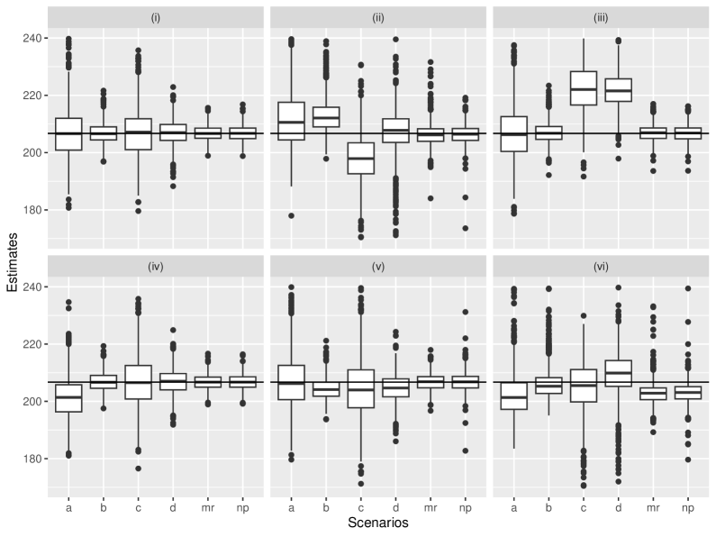
Figure S2: Simulation results for estimators of $\theta_{00}^{(10)}$ among 6 different scenarios with sample size $n=1,000$. Scenarios (i)–(vi) are described in Section 4.6. The horizontal line in each panel is the true value of $\theta_{00}^{(10)}$.

References

- Albert and Nelson (2011) Albert, J. M. and Nelson, S. (2011), “Generalized causal mediation analysis,” Biometrics, 67, 1028–1038.
- Andrews (1991) Andrews, D. W. (1991), “Asymptotic normality of series estimators for nonparametric and semiparametric regression models,” Econometrica: Journal of the Econometric Society, 307–345.
- Angrist et al. (1996) Angrist, J. D., Imbens, G. W., and Rubin, D. B. (1996), “Identification of causal effects using instrumental variables,” Journal of the American Statistical Association, 91, 444–455.
- Bickel et al. (1993) Bickel, P. J., Klaassen, C. A., Bickel, P. J., Ritov, Y., Klaassen, J., Wellner, J. A., and Ritov, Y. (1993), Efficient and adaptive estimation for semiparametric models, volume 4, Springer.
- Chen and White (1999) Chen, X. and White, H. (1999), “Improved rates and asymptotic normality for nonparametric neural network estimators,” IEEE Transactions on Information Theory, 45, 682–691.
- Cheng et al. (2021) Cheng, C., Spiegelman, D., and Li, F. (2021), “Estimating the natural indirect effect and the mediation proportion via the product method,” BMC Medical Research Methodology, 21, 1–20.
- Cheng et al. (2023) — (2023), “Is the product method more efficient than the difference method for assessing mediation?” American Journal of Epidemiology, 192, 84–92.
- Chernozhukov et al. (2018) Chernozhukov, V., Chetverikov, D., Demirer, M., Duflo, E., Hansen, C., Newey, W., and Robins, J. (2018), “Double/debiased machine learning for treatment and structural parameters: Double/debiased machine learning,” The Econometrics Journal, 21.
- Daniel et al. (2015) Daniel, R. M., De Stavola, B. L., Cousens, S., and Vansteelandt, S. (2015), “Causal mediation analysis with multiple mediators,” Biometrics, 71, 1–14.
- Díaz et al. (2021) Díaz, I., Hejazi, N. S., Rudolph, K. E., and van Der Laan, M. J. (2021), “Nonparametric efficient causal mediation with intermediate confounders,” Biometrika, 108, 627–641.
- Ding and Lu (2017) Ding, P. and Lu, J. (2017), “Principal stratification analysis using principal scores,” Journal of the Royal Statistical Society. Series B (Statistical Methodology), 757–777.
- Forastiere et al. (2018) Forastiere, L., Mattei, A., and Ding, P. (2018), “Principal ignorability in mediation analysis: through and beyond sequential ignorability,” Biometrika, 105, 979–986.
- Frangakis and Rubin (1999) Frangakis, C. E. and Rubin, D. B. (1999), “Addressing complications of intention-to-treat analysis in the combined presence of all-or-none treatment-noncompliance and subsequent missing outcomes,” Biometrika, 86, 365–379.
- Frangakis and Rubin (2002) — (2002), “Principal stratification in causal inference,” Biometrics, 58, 21–29.
- Frölich and Huber (2017) Frölich, M. and Huber, M. (2017), “Direct and indirect treatment effects–causal chains and mediation analysis with instrumental variables,” Journal of the Royal Statistical Society. Series B (Statistical Methodology), 1645–1666.
- Frölich and Melly (2013) Frölich, M. and Melly, B. (2013), “Identification of treatment effects on the treated with one-sided non-compliance,” Econometric Reviews, 32, 384–414.
- Hines et al. (2022) Hines, O., Dukes, O., Diaz-Ordaz, K., and Vansteelandt, S. (2022), “Demystifying statistical learning based on efficient influence functions,” The American Statistician, 76, 292–304.
- Imai et al. (2010a) Imai, K., Keele, L., and Tingley, D. (2010a), “A general approach to causal mediation analysis.” Psychological Methods, 15, 309.
- Imai et al. (2010b) Imai, K., Keele, L., and Yamamoto, T. (2010b), “Identification, Inference and Sensitivity Analysis for Causal Mediation Effects,” Statistical Science, 25, 51–71.
- Jiang et al. (2022) Jiang, Z., Yang, S., and Ding, P. (2022), “Multiply robust estimation of causal effects under principal ignorability,” Journal of the Royal Statistical Society Series B: Statistical Methodology, 84, 1423–1445.
- Jo (2022) Jo, B. (2022), “Handling parametric assumptions in principal causal effect estimation using Gaussian mixtures,” Statistics in Medicine, 41, 3039–3056.
- Jo and Stuart (2009) Jo, B. and Stuart, E. A. (2009), “On the use of propensity scores in principal causal effect estimation,” Statistics in Medicine, 28, 2857–2875.
- Kang and Schafer (2007) Kang, J. D. and Schafer, J. L. (2007), “Demystifying Double Robustness: A Comparison of Alternative Strategies for Estimating a Population Mean from Incomplete Data,” Statistical Science, 22, 523–539.
- Kim et al. (2017) Kim, C., Daniels, M. J., Marcus, B. H., and Roy, J. A. (2017), “A framework for Bayesian nonparametric inference for causal effects of mediation,” Biometrics, 73, 401–409.
- Lee et al. (1991) Lee, Y. J., Ellenberg, J. H., Hirtz, D. G., and Nelson, K. B. (1991), “Analysis of clinical trials by treatment actually received: is it really an option?” Statistics in Medicine, 10, 1595–1605.
- Miles et al. (2017) Miles, C. H., Shpitser, I., Kanki, P., Meloni, S., and Tchetgen Tchetgen, E. J. (2017), “Quantifying an adherence path-specific effect of antiretroviral therapy in the Nigeria PEPFAR program,” Journal of the American Statistical Association, 112, 1443–1452.
- Miles et al. (2020) — (2020), “On semiparametric estimation of a path-specific effect in the presence of mediator-outcome confounding,” Biometrika, 107, 159–172.
- Nguyen et al. (2021) Nguyen, T. Q., Schmid, I., and Stuart, E. A. (2021), “Clarifying causal mediation analysis for the applied researcher: Defining effects based on what we want to learn.” Psychological Methods, 26, 255.
- Park and Kürüm (2018) Park, S. and Kürüm, E. (2018), “Causal mediation analysis with multiple mediators in the presence of treatment noncompliance,” Statistics in Medicine, 37, 1810–1829.
- Park and Kürüm (2020) — (2020), “A two-stage joint modeling method for causal mediation analysis in the presence of treatment noncompliance,” Journal of Causal Inference, 8, 131–149.
- Park and Palardy (2020) Park, S. and Palardy, G. J. (2020), “Sensitivity Evaluation of Methods for Estimating Complier Average Causal Mediation Effects to Assumptions,” Journal of Educational and Behavioral Statistics, 45, 475–506.
- Pearl (2001) Pearl, J. (2001), “Direct and indirect effects,” in Proceedings of the Seventeenth Conference on Uncertainty and Artificial Intelligence, 2001, Morgan Kaufman, 411–420.
- Price et al. (1992) Price, R. H., Van Ryn, M., and Vinokur, A. D. (1992), “Impact of a preventive job search intervention on the likelihood of depression among the unemployed,” Journal of Health and Social Behavior, 158–167.
- Robins and Richardson (2010) Robins, J. M. and Richardson, T. S. (2010), “Alternative graphical causal models and the identification of direct effects,” in Causality and Psychopathology: Finding the Determinants of Disorders and Their Cures, 103–158.
- Rosenbaum and Rubin (1983) Rosenbaum, P. R. and Rubin, D. B. (1983), “The central role of the propensity score in observational studies for causal effects,” Biometrika, 70, 41–55.