Ly$\alpha$ at Cosmic Dawn with a Simulated Roman Grism Deep Field

Abstract

The slitless grism on the Nancy Grace Roman Space Telescope will enable deep near-infrared spectroscopy over a wide field of view. We demonstrate Roman’s capability to detect Ly$\alpha$ galaxies at $z>7$ using a multi-position-angle (PA) observational strategy. We simulate Roman grism data using a realistic foreground scene from the COSMOS field. We also input fake Ly$\alpha$ galaxies spanning redshift z=7.5-10.5 and a line-flux range of interest. We show how a novel data cube search technique – CUBGRISM – originally developed for GALEX can be applied to Roman grism data to produce a Ly$\alpha$ flux-limited sample without the need for continuum detections. We investigate the impact of altering the number of independent PAs and exposure time. A deep Roman grism survey with 25 PAs and a total exposure time of $70$hrs can achieve Ly$\alpha$ line depths comparable to the deepest $z=7$ narrow-band surveys ($L_{{\rm{Ly}}\alpha}\gtrsim 10^{43}$erg s^-1). Assuming a null result, where the opacity of the intergalactic medium (IGM) remains unchanged from $z\sim 7$, this level of sensitivity will detect $\sim 400$ deg^-2 Ly$\alpha$ emitters from $z=7.25-8.75$. A decline from this expected number density is the signature of an increasing neutral hydrogen fraction and the onset of reionization. Our simulations indicate that a deep Roman grism survey has the ability to measure the timing and magnitude of this decline, allowing us to infer the ionization state of the IGM and helping us to distinguish between models of reionization.

1 Introduction

Ly$\alpha$ emission is a bright spectral feature in star-forming galaxies that many observational surveys have targeted to efficiently obtain large samples of Ly$\alpha$ emitting galaxies over a wide redshift range $z=2-7$ (e.g., Cowie & Hu, 1998; Rhoads et al., 2000; Malhotra & Rhoads, 2002; Ouchi et al., 2003; Gawiser et al., 2007; Gronwall et al., 2007; Blanc et al., 2011; Finkelstein et al., 2013; Konno et al., 2014; Matthee et al., 2015; Tilvi et al., 2020). With the arrival of JWST, Ly$\alpha$ continues to play an essential role in the study of high-redshift galaxies and the ionization state of the intergalactic medium (IGM) (Endsley et al., 2022; Tang et al., 2023; Bunker et al., 2023; Saxena et al., 2023). The most exciting JWST Ly$\alpha$-observation to date is the discovery of an emitter at z=10.6 (Bunker et al., 2023). This object shows that Ly$\alpha$ can find a way to escape only $430$ Myr after the Big Bang, where even extremely early reionization models (e.g., Finkelstein et al., 2019) predict a neutral hydrogen fraction of $\sim 80\%$. However, the current Ly$\alpha$ JWST observations are limited in volume and are pre-selected based on broadband criteria. We need a deep, blind search for Ly$\alpha$ over a large volume to realize the full potential of Ly$\alpha$-based reionization constraints.

We know that reionization should fall within the $6<z<9$ redshift range from the saturation of Ly$\alpha$ absorbers in $z\sim 6$ quasar spectra (Fan et al., 2006) and by polarization measurements of the cosmic microwave background (Planck Collaboration et al., 2018). To go beyond this rough picture, many groups have used the redshift evolution of the number density of Ly$\alpha$ emitters (LAEs) to constrain the timing of reionization. Some groups have found a large drop in their density at $z\sim 7$ and have attributed this decline to the increasing opacity of the IGM and the onset of the epoch of reionization (e.g., Stark et al., 2010; Konno et al., 2014; Hoag et al., 2019), while other groups have found a more modest evolution over this same redshift range consistent with a largely ionized universe (e.g., Tilvi et al. 2010; Itoh et al. 2018; Zheng et al. 2017; Hu et al. 2019; Wold et al. 2022). Some of the variation in the results may be due to spatially inhomogeneous reionization since cosmological reionization is thought to have proceeded through the growth and eventual overlap of ionized bubbles, driven by ultraviolet photon production in the earliest galaxies. This produces a non-uniform reionization history that necessitates observational studies with large survey volumes to mitigate cosmic variance.

The current variation and uncertainty in the observational constraints allow for a diverse set of reionization histories. These reionization scenarios range from a rapid neutral-to-ionized transition dominated by relatively massive galaxies (Naidu et al., 2020) to a gradual transition dominated by more numerous low-mass galaxies (Finkelstein et al., 2019). The redshift where these reionization models differ the most is $z\sim 8$. For example, at this redshift Naidu et al. predict an almost fully neutral universe, while the Finkelstein et al. model predicts a much lower neutral fraction of $35\%$. Moving to lower (higher) redshifts the models converge to a fully ionized (neutral) IGM, making $z\sim 8$ an ideal redshift to distinguish between models and tell us about the sources of ionization radiation - whether large galaxies or small.

However, it is difficult to obtain $z\sim 8$ Ly$\alpha$-based observational constraints from ground facilities largely due to the increasing night sky background and the need for expensive spectroscopic followup of Ly$\alpha$ candidates to eliminate contamination. To effectively study reionization at $z\sim 8$, we need to acquire greater statistical leverage by obtaining spectroscopically complete samples of LAEs over larger volumes without the interference of the Earth’s atmosphere.

In this paper, we investigate Roman’s potential to obtain a LAE sample at $z\gtrsim 7$ with a multi-position-angle grism deep field. Roman’s Wide Field Instrument (WFI) has visible to near-infrared imaging capability and a slitless grism capability spanning a wavelength range of $1.00-1.93$ $\mu$m with an $\sim 11$ Å per pixel dispersion. The WFI has a field of view of $0.281$ square degrees or over 100 times larger than similar instruments on HST and JWST. This large field-of-view (FOV) is tiled by 18 detectors in 3 rows and 6 columns with a $0.11^{\prime\prime}$ pixel scale. It is the combination of Roman’s wide field of view and grism wavelength range that will clear the way for $z>7$ LAE searches with unprecedented volumes – a volume of $\sim 3\times 10^{6}$ Mpc³ from $z=7.25$ to $8.75$ in a single pointing.

Slitless grism capabilities are well suited for space-based telescopes where the sky background is low, and where slitless modes are often the simplest way to add spectroscopy to a mission. Furthermore, slitless observations are extremely efficient at spectroscopic surveys because all objects within the field-of-view have their light dispersed across the detector. This is particularly a desirable feature for finding strong emission line sources that are easily missed in slit-mask observations which often select their targets based on continuum brightness (Malhotra et al., 2005; Tilvi et al., 2016; Larson et al., 2018).

These strengths also present challenges. In particular, neighboring sources aligned in the dispersion direction can have overlapping spectra. This means that a high-redshift slitless grism survey will need to contend with contamination caused by the foreground scene of stars and galaxies, and a simple exposure time calculation will fail to capture the true survey performance given this source confusion. For these reasons, we simulate a realistic extra-galactic foreground scene that captures the key characteristics of a grism deep field and then assess our ability to conduct a blind search for Ly$\alpha$ galaxies at cosmic dawn. We show how a novel data cube search technique – CUBGRISM – originally developed for GALEX grism data can be applied to Roman data allowing us to isolate $z>7$ Ly$\alpha$ galaxies.

2 Grism Simulations

We use HST imaging and best-fit SEDs in the COSMOS field to define our simulated foreground stars and galaxies. We also construct fake high-redshift ($7.5<z<10.5$) Ly$\alpha$ emitters with a variety of intrinsic characteristics and then measure our ability to detect these emitters with different observational strategies. In the following sections, we describe the construction of our grism simulations in detail.

2.1 Foreground Scene

Our simulated foreground objects are populated based on HST observations of the COSMOS field. Specifically, we use the version-4.1 3D-HST COSMOS F160W mosaic with the derived photometric and EAZY output files that are publicly available via the 3D-HST collaboration (Skelton et al., 2014; Brammer et al., 2012; Grogin et al., 2011; Koekemoer et al., 2011). The HST COSMOS field has a $\sim 9\times 22$ arcmin² field of view observed with 44 filter bandpasses including 5 HST filters: F606W, F814W, F125W, F140W, and F160W with $5\sigma$ depths of 26.7, 26.5, 26.1, 25.5, and 25.8, respectively (Skelton et al., 2014).

2.1.1 Morphology

We define the morphology of simulated objects with image postage stamps. We use the 3D-HST F160W mosaic to make these images for all of our simulated foreground sources. For each object, we extract a sub-image from the science F160W image centered on the object’s coordinates, where all pixels not assigned to the object via the segmentation map are zeroed out. To prepare these sub-images for input, we resample the F160W mosaic’s drizzled pixel scale of $0.06^{\prime\prime}$ to match Roman’s pixel scale of $0.11^{\prime\prime}$. Note, the native pixel scale of WFC3-IR is about $0.13^{\prime\prime}$/pixel, so we’re producing a final model image with a pixel scale very near the actual input data. The F160W mosaic has a median $5\sigma$ depth of 25.8 mag and an average FWHM of $0.19^{\prime\prime}$ (Skelton et al., 2014). Our foreground simulations include all F160W objects with magnitudes brighter than 25.5 mag. This corresponds to the expected $1\sigma$ per pixel sensitivity at $1.5\mu$m for our deepest simulated Roman grism survey with a total $t_{{\rm{exp}}}=69.4$ hrs.

2.1.2 Spectra

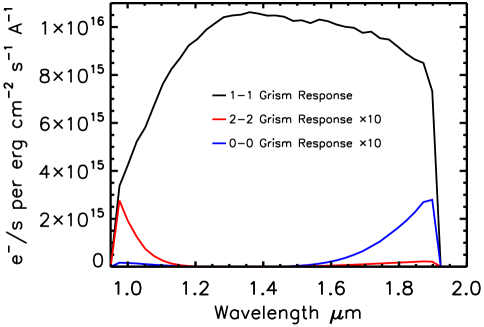
Figure 1: Roman WFI grism response functions for the in-focus spectral orders. For display purposes, we increased the 2-2 and 0-0 grism response functions by a factor of ten. All three in-focus spectral orders are included in our grism simulations.

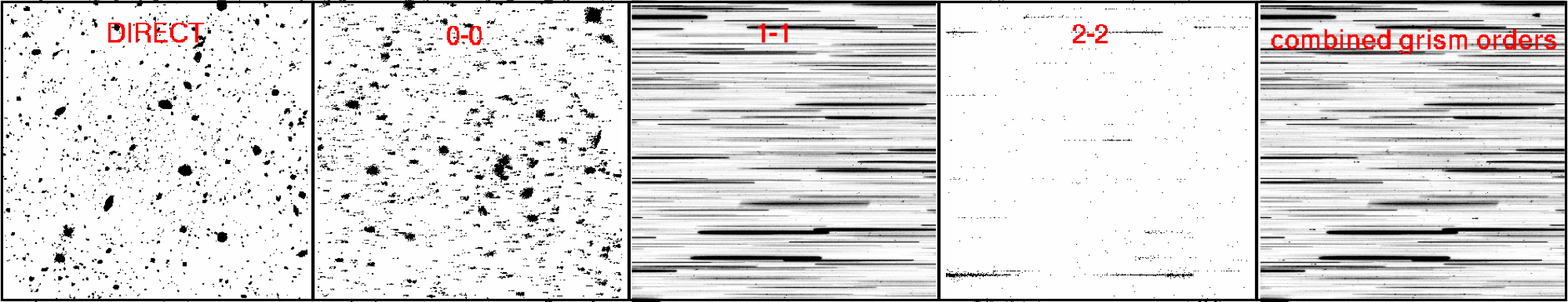
Figure 2: Construction of the noiseless simulated grism images. All the in-focus spectral orders: 0-0, 1-1, and 2-2 are simulated independently and then co-added to form our combined grism image. Finally, we add in the Poisson noise appropriate to our desired exposure time (see Figure 3). For the four panels above, we show a $3.75\times 3.75^{\prime}$ field of view.

We use the best-fit EAZY SEDs from Skelton et al. (2014) to define the spectra of all the simulated foreground objects. These spectral templates were fit to 44 bandpasses with 13 spanning our simulated $1$ to $2$ $\mu$m wavelength range. Skelton et al. find excellent agreement with their photometric redshifts and the available spectroscopic redshifts, with a scatter of $\sigma_{{\rm{NMAD}}}=0.007$ and an outlier percentage of $1\%$. This level of agreement suggests that their templates SEDs, which we use directly, are able to accurately represent the spectral data.

For our Roman grism simulations, we are most concerned with reproducing a realistic foreground scene for the $1$ to $2$ $\mu$m wavelength range, and we normalize the EAZY SEDs to the observed F160W photometry to help ensure that our simulated grism image has a realistic distribution of foreground flux.

2.2 Simulated Ly$\alpha$ emitters

Simulated Ly$\alpha$ emitters are populated with a range of redshifts: $z=\{7.5,8.5,9.5,10.5\}$, lines fluxes: $f_{{\rm{Ly}\alpha}}=\{0.45,0.6,1.0,1.2,4.0,7.0\times 10^{-17}$ erg s^-1cm${}^{-2}\}$, continuum magnitudes: $m_{{\rm{F160W}}}=\{25.5,26.5,27.5,28.5\}$, and morphologies: half-light radii $=0.17\pm 0.02^{\prime\prime}$. To achieve realistic Ly$\alpha$ morphologies, each object’s semi-major and semi-minor axis lengths are uniformly selected over an interval spanning from 2 to 5 Roman pixels. This randomly selected size is then paired with an F160W cataloged source with a matching spatial extent. This observed F160W source is then used to generate the needed image postage stamp as discussed in Section 2.1.1. The end result is distribution with $\left\langle r_{{\rm 1/2}}\right\rangle\pm 1\sigma=0.17\pm 0.02^{\prime\prime}$ which is consistent with the expected size of $z\gtrsim 7$ LAEs (Malhotra et al., 2012; Allen et al., 2017; Shibuya et al., 2019; Kim et al., 2021; Rhoads et al., 2023).

For the Ly$\alpha$ spectral shape, the continuum has a spectral slope of $-2$ such that $f_{\lambda}\varpropto\lambda^{-2}$ and is attenuated by the intervening IGM. The Ly$\alpha$ line is a Gaussian with rest-frame FWHM$=1$Å or 250 km s^-1 which is consistent with observational constraints (Hu et al., 2010). We insert a total of $288$ Ly$\alpha$ emitters into our foreground grism scene. To ensure that all position angles contain our simulated emission lines, we randomly place our Ly$\alpha$ emitters within a radius of $1$ arcmin of the field center.

2.3 Simulation Construction

We use the aXeSIM (Kümmel et al., 2009) software package to simulate 25 independent position angles over a $2048\times 2048$ pixel or 14.1 arcmin² field of view. aXeSIM was originally designed to simulate grism and direct images for the Hubble Space Telescope and a number of modifications were needed to simulate Roman data. We modified aXe’s instrument parameter file to match Roman’s trace and wavelength dispersion. We simulated a wavelength range of $9500-19000$ Å and assumed a constant wavelength dispersion of $265.7$, $10.8$, and $5.6$ Å pix^-1 for orders 0-0, 1-1, and 2-2, respectively. We set the zero deviation wavelength of the 1-1 order to be $0.95\mu$m, which differs from Roman’s undeviated wavelength of $\sim 1.55\mu$m. Given the field of view of the input scene relative to our smaller simulated region, we do not expect this difference to impact our measurement of recovery fractions for simulated Ly$\alpha$ emitters.

We used the morphological and spectral inputs described in the previous sections to run three separate aXe simulations to form grism images for Roman’s 0-0, 1-1, and 2-2 spectral orders. To further facilitate parallelization and to allow for alterations to our Ly$\alpha$ emitter sample, we simulated the grism foreground scene separately from the simulated LAE grism images.

In Figure 1, we show the Roman grism response functions that we used in our aXe simulations. Compared to the science 1-1 order, the 0-0 and 2-2 orders have less-sensitive response functions. However, these orders can significantly complicate the foreground scene. The 0-0 order is compact with the full $1\mu$m grism range only occupying tens of pixels. A compact 0-0 order from a bright foreground object may be mistaken as an emission line, and we wish to verify that our LAE search does not select these potential contaminants. The 2-2 order is spread out over $\sim 2000$ pixels, about twice the length of the science order. This means that bright objects well outside of the simulated FOV can have their 2-2 light dispersed into the grism image and contribute to the foreground flux that we need to contend with when searching for high-redshift LAEs.

In Figure 2, we show an example of our simulated spectral orders and their summation for a position angle (PA) aligned with the x-axis or PA$=0$ by aXe convention. Non-zero position angles are not naturally supported by the aXe simulation software. Thus, we rotated all objects’ morphologies and positions about the field center to simulate position angles not equal to zero.

Once all three spectral order simulations were completed for both the foreground and LAE scene, we combined them and applied a Poisson noise level of $0.8$ $e^{-}$pix^-1s^-1 which is the expected near-infrared background for the High Latitude Survey (see Figure 3). For our deepest simulated Roman grism survey, we explored an observational strategy consisting of $25$ exposures – each with a unique PA – observed for $10$ ks giving a total exposure time of $69.4$ hours. The simulated PAs were selected to uniformly sample 360 degrees, while avoiding 180 degree reflections. This was done because PA₀ and PA${}_{0}+180$ will have largely the same spectra that are aligned and overlapping, complicating our effort to deblend sources.

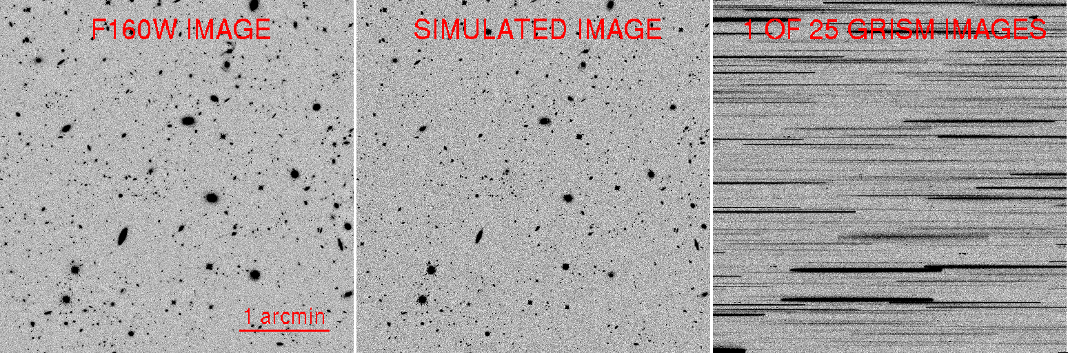
Figure 3: Left: Observed HST F160W image. Middle: Our simulated F160W image. Right: Our simulated Roman grism image with a position angle aligned with the x-axis. For our deep field simulations, we consider up to 25 independent position angles and up to 69.4 hours of total integration time. We use a noise level of $0.8$ $e^{-}$pix^-1s^-1 which is the expected near-infrared background for the High Latitude Survey.

We also investigated two lesser surveys: one with 25 PAs and a total exposure time of 41.7 hours ($25\times 6$ ks) and another with a subset of 15 PAs and the same total exposure time of 41.7 hours ($15\times 10$ ks). For brevity, we refer to these three scenarios as $25\times 10$ ks, $25\times 6$ ks, $15\times 10$ ks.

2.4 Simulation Caveats

Roman’s wide field slitless spectroscopy with a wavelength dispersion of $\sim 11$ Å per pixel over a $1$ $\mu$m range is achieved with a compound grism with two diffractive surfaces. This grism assembly mitigates wavelength-dependent aberrations at the expense of producing additional unwanted spectral orders. Our simulations are designed to capture the grism characteristics most relevant for a deep LAE survey. In particular, we aim to assess Roman’s ability to conduct a deep LAE survey given a realistic foreground scene. Accordingly, we simulate the spectral off-orders that have the highest surface brightness (0-0 and 2-2) and ignore out-of-focus spectral orders (1-0, 1-2, 0-1, 2-1). Additionally, we do not model field-dependent distortions of the spectral trace or dispersion which are expected to have a minor impact on the performance of a deep LAE survey.

Our simulations are designed to predict the needed on-target time to perform a deep LAE survey, and we do not investigate different dithering/mosaicing strategies. For simplicity, all 25 simulated PAs are assigned the same field center maximizing the area that is covered by all PAs.

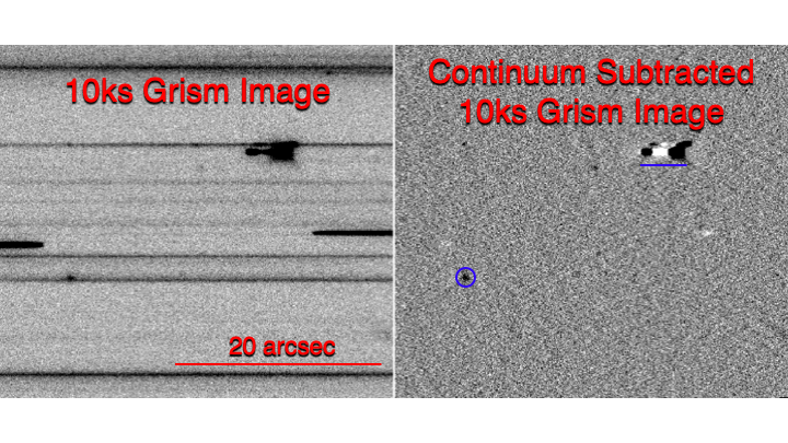
Figure 4: We show a small $40\times 40^{\prime\prime}$ region of our simulated $t_{\rm{exp}}=10$ks grism image before and after continuum subtraction. We have highlighted a foreground emission line galaxy (blue circle) and an artifact caused by the 0-0 order of a bright star (underlined in blue). See Section 3.1 for additional discussion of our continuum subtraction method. We demonstrate that our emission line search technique, CUBGRISM, can effectively remove contamination from 0-0 spectra and recover a clean sample of emission line sources.

3 CUBGRISM

We use a novel data cube search technique - CUBGRISM - originally developed for GALEX grism data to test our ability to recover high-redshift Roman LAEs. This technique does not require a broad-band detection and was constructed to produce a line-flux limited sample of emission-line objects. These features are well-tailored to our goal of characterizing our ability to recover Ly$\alpha$ emitters given an assumed Roman grism deep field observing strategy.

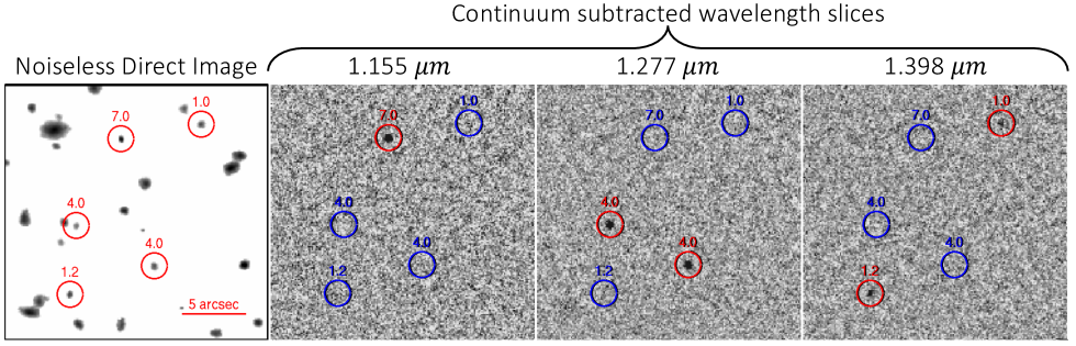
Figure 5: A $20^{\prime\prime}\times 20^{\prime\prime}$ region of our simulated Roman direct image and three selected wavelength slices from our data cube constructed from 25 Roman grism images. From left to right, we show the Roman direct image, a 1.155 $\mu$m data cube slice containing 1 simulated $z=8.5$ LAE, a 1.277 $\mu$m data cube slice containing 2 simulated $z=9.5$ LAEs, and a 1.398 $\mu$m data cube slice containing 2 simulated $z=10.5$ LAEs. The simulated LAEs are circled in red. The number associated with each LAE indicates the line-flux of the source, where the Ly$\alpha$ flux is in units of $10^{-17}$erg s^-1cm^-2. By design continuum sources are not recovered in our data cube due to our background subtraction procedure (see Section 3 for details).

3.1 Continuum Subtraction

In preparation for the data cube construction and our emission line search, we subtracted continua from the grism images by applying a $1\times 21$ pixel median filter with the $21$ pixel dimension aligned with the spectral trace. The size of the median filter ($21$ pixels or $231$Å) is designed to not bias our search for LAEs which will have FHWMs a factor of $\gtrsim 20$ smaller. In Figure 4, we demonstrate our continuum subtraction method showing that the remaining sources are primarily emission lines (both simulated LAEs and foreground sources) and 0-0 spectra.

3.2 Cube Construction

In Barger et al. (2012); Wold et al. (2014, 2017), we describe CUBGRISM (previously referred to as the data cube search) in detail and demonstrate our method for converting multiple slitless spectroscopic images into a three-dimensional data cube with two spatial axes and one wavelength axis. Here, we provide a brief overview of this process with emphasis on alterations needed for Roman grism images.

For each simulated grism exposure, we know the spectral trace and wavelength dispersion, and this allows us to extract a spectrum for each spatial pixel position, thus forming an initial data cube. A data cube constructed from a single slitless spectroscopic image may suffer from overlapping spectra caused by neighboring objects that are oriented in line with the dispersion direction. For our simulated Roman deep field, we have multiple position angles - one per exposure - and objects that overlap in one position angle are unlikely to overlap in another position angle. This allows us to disentangle overlaps by constructing data cubes for each exposure and then combining these initial data cubes, applying a 5$\sigma$ cut to remove contamination from overlapping sources. In more detail, we take our library of data cubes ($N=25$ for our deep survey) and for each spaxel location, we measure the variation in flux values, quantified by the normalized median absolute deviation. Any spaxel that deviates from the median by more than $5\sigma$ is eliminated and the remaining spaxels are used to compute the median flux value which is then used to populate the final data cube.

This procedure results in a final data cube that has a wavelength step of 10 Å and wavelength coverage of approximately 1.0–1.5 $\mu$m. We designed the wavelength slices to have a wavelength extent that matches the spectral resolution of the Roman Space Telescope. We are interested in our ability to recover high-redshift Ly$\alpha$ emitters ($z=7.5$–$10.5$), and accordingly, we artificially limit the wavelength range of the output data.

3.3 Line Search

The final Roman data cubes cover a wavelength range of 1.00 to 1.49 $\mu$m or a Ly$\alpha$ redshift range of $z=7.24-11.25$. For each wavelength slice, we used SExtractor (SE; Bertin & Arnouts, 1996) to identify $>7.5\sigma$ detections using SNR-optimised aperture photometry. We computed an optimal aperture size of $D=0.4^{\prime\prime}$ by determining the aperture that maximizes the median Ly$\alpha$ data-cube flux relative to the measured aperture noise (for details on SNR-optimal apertures, see Gawiser et al., 2006). As discussed in the next section, this level of significance ($>7.5\sigma$) is needed to minimize false detections within the cube.

3.4 False detections

CUBGRISM enables a blind search for Ly$\alpha$ emitters – with no continuum detection required – at the expense of requiring a PA-rich observational strategy to accurately isolate emitter locations. We favor this continuum-independent reduction strategy because our science goals require us to compare Roman Ly$\alpha$ populations at cosmic dawn to blind Ly$\alpha$ narrow-band searches just outside the reionization epoch at $z\lesssim 7$ (Ouchi et al., 2008, 2010; Shibuya et al., 2012; Konno et al., 2014, 2018; Matthee et al., 2015; Santos et al., 2016; Ota et al., 2017; Itoh et al., 2018; Hu et al., 2019, 2021; Tilvi et al., 2020; Wold et al., 2022).

However, for reduced PA observational strategies, a potential drawback of our technique is the inability to isolate source locations resulting in spurious detections.

CUBGRISM has been used successfully on GALEX grism deep fields observed with hundreds of PAs to identify populations of low-redshift Ly$\alpha$ emitters. These far-ultraviolet and near-ultraviolet surveys found a high optical-spectroscopic confirmation rate of $85\%$ (Wold et al., 2014, 2017). In addition to a $4\sigma$ detection within data cube, these GALEX studies also visually inspected profile-weighted one-dimensional spectra to help eliminate spurious detections. For our Roman simulations, we did not implement a hard-to-quantify visual inspection step. Instead, we verify that our adopted CUBGRISM extraction parameters result in a manageable contamination rate ($\lesssim 15\%$) which would likely be improved with a visual inspection or machine learning step.

Table 1: Roman Grism Survey Performance

Total	Number	Average survey	False	Figure 6
Exposure	of	Flux Limit	Detection	symbol
Time (hrs)	PAs	($\times 10^{-18}$ erg s-1cm-2)	Fraction	color
69.4	25	8.2$\pm$0.7	0.137$\pm$0.048	red
41.7	25	10.8$\pm$0.6	0.074$\pm$0.069	green
41.7	15	10.4$\pm$0.5	0.058$\pm$0.055	blue
41.7	10	10.2$\pm$0.6	0.678$\pm$0.035	$\cdots$

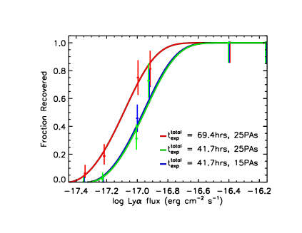
Figure 6: The fraction of recovered Ly$\alpha$ emitters as a function of line-flux. Error-bars show the $1\sigma$ Poisson error. The red, green, and blue curves show examples of how our survey completeness varies with different observational strategies assuming a $0.8$ $e^{-}$pix^-1s^-1 background noise level typical of the High Latitude Survey (see Section 4 for details).

For a deep Roman grism survey, we aim to detect the Ly$\alpha$ number density decline caused by the increasing opacity of the IGM and the onset of reionization. As a baseline for determining the rate of false detections, we define the false detection fraction as $F/(F+E)$ where $F$ is the number of recovered spurious objects within the $z_{\rm{Ly\alpha}}=7.25$–$8.75$ redshift range and $E$ is the number of expected LAEs over the same redshift range assuming no number density evolution from the $z\sim 7$ LAGER survey (e.g., Wold et al., 2022; Hu et al., 2019). Given our survey flux limits, we expect a $69.4$ hr survey to detect $N\sim 400$ LAEs while our $41.7$ hr surveys should detect $N\sim 150$ LAEs over a nominal deep grism survey area of $1$ deg² (see Section 4 for details).

It is not possible to simulate a larger $\sim 1$ deg² FOV because of the limited HST near-infrared imaging data and our COSMOS observation-based simulations. Instead, we assume that our limited FOV is representative and perturb our simulations with different realizations of Poisson noise. For each realization, we find the number of false detections over a wavelength range of 1.00 to 1.19 $\mu$m, which corresponds to the wavelength range of observed $z=7.25$–$8.75$ Ly$\alpha$ emission. In total, we look for false detections over an effective survey area 350 arcmin² and consider all three survey scenarios: $25\times 10$ ks, $25\times 6$ ks, $15\times 10$ ks.

For all three survey configurations, we find that a $7.5\sigma$ detection threshold can keep the false detection rate at $\lesssim 15\%$. In Table 1, we summarize these results with their $1\sigma$ Poisson errors. We caution that using $N\ll 15$ PAs will result in reduced performance of our CUBGRISM reduction strategy. Using the same procedure as employed with the $25\times 10$ ks, $25\times 6$ ks, and $15\times 10$ ks surveys, we estimate that a $10\times 15$ ks PA survey would result in a $\sim 70\%$ false detection rate. Reduced performance with a PA-poor survey is expected because of CUBGRISM’s method of disentangling overlapping spectra (described in Section 3.2) which requires many PAs to measure the uncontaminated flux at each $x,y,\lambda$ position.

We note that our false detection results do not account for foreground emission-line contamination. We assume that a deep Roman grism survey will be located in a field that contains deep ancillary imaging data that are capable of efficiently identifying foreground objects. As performed in the GALEX grism and narrow-band Ly$\alpha$ surveys, the false detection rate can be further investigated by independently confirming a representative subset of identified Roman grism Ly$\alpha$ emitters.

4 Results

Given our generated realistic foreground scene and our reduction strategy, we now determine the recovery fraction of simulated Ly$\alpha$ emitters as a function of line-flux, redshift, and number of position angles. In Figure 5, we demonstrate this Ly$\alpha$ search by highlighting a small $20^{\prime\prime}\times 20^{\prime\prime}$ region of our deepest simulation that contains 5 LAEs with different line fluxes and redshifts. For each wavelength slice, we search for LAEs and record the Ly$\alpha$ recovery fraction as a function of line flux.

As discussed in Section 2.3, we focused our investigation on three different deep-field scenarios.

1. 25 PAs with a total exposure time of 69.4 hours ($25\times 10$ ks)

2. 25 PAs with a total exposure time of 41.7 hours ($25\times 6$ ks)

3. 15 PAs with a total exposure time of 41.7 hours ($15\times 10$ ks)

For each scenario, we show the fraction of recovered LAEs as a function of line-flux in Figure 6. Following Negrello et al. (2013), we fit our recovery fractions with an error function

$$R(f_{{\rm{Ly}\alpha}})={\rm{erf}}[(logf_{{\rm{Ly}\alpha}}-logf)^{2}/\gamma^{2}]$$ (1)

where $logf$ and $\gamma$ are free parameters that control the location of the zero-to-one transition and the rate of this transition, respectively. We find that the $\gamma$ parameter is very similar for all curves, and we fix its value to the $25\times 10$ ks best-fit value of $\gamma=0.52$. Based on these best-fit functions, we find that our three scenarios are $50\%$ complete at a Ly$\alpha$ line fluxes of $8.2$, $10.8$, and $10.4\times 10^{-18}$ erg s^-1cm^-2, respectively. This is consistent with the survey depth increasing proportionally to the square root of the total exposure time. In Table 1, we list our surveys’ flux completeness with $1\sigma$ errors computed with a Monte Carlo (MC) procedure that perturbs our completeness data-points by Poisson random deviates. This MC procedure is used to create $N=10,000$ perturbed completeness curves and the measured variation in the survey completeness is used to estimate the $1\sigma$ error.

We investigate Roman’s Ly$\alpha$ survey depth as a function of redshift for our deepest $25\times 10$ ks survey configuration. Binning by line flux and redshift reduce the number of simulated LAEs per bin by a factor of four when compared to binning by line flux alone. To reduce the Poisson error in our recovery fraction results, we have produced four Ly$\alpha$ samples while keeping our foreground scene the same. For each Ly$\alpha$ sample, we independently select Ly$\alpha$ parameters as described in Section 2.2. This includes randomly selecting their positions. For each run, the Ly$\alpha$ sample is added to the foreground scene and Poisson noise is added. We combine Ly$\alpha$ recovery results from all four runs to compute the final completeness curves.

Table 2: Deep Roman Grism Survey Redshift Performance

Redshift	Flux Limit	Luminosity Limit	Figure 7
	($\times 10^{-18}$ erg s-1cm-2)	($\times 10^{42}$ erg s-1)	symbol color
7.5	13.6$\pm$0.8	9.1$\pm$0.6	magenta
8.5	8.3$\pm$0.4	7.4$\pm$0.4	cyan
9.5	7.5$\pm$0.4	8.6$\pm$0.4	yellow
10.5	6.9$\pm$0.4	9.9$\pm$0.6	orange

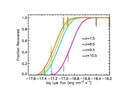
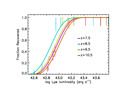
Figure 7: Left: For our deepest grism simulation ($t_{{\rm{exp}}}=69.4$ hrs), we show Ly$\alpha$ flux completeness curves for different emitter redshifts. Right: Same as the left figure except completeness is plotted versus Ly$\alpha$ luminosity. Across all redshift bins, we find that our survey can recover $L_{{\rm{Ly}}\alpha}>10^{43}$ erg s^-1 LAEs at the $50\%$ completeness level (see Table 2).

In Figure 7, we show these redshift-dependent Ly$\alpha$ recovery fractions. From $z=7.5$ to $10.5$, we find that our survey is $50\%$ complete at Ly$\alpha$ line fluxes of $13.6$, $8.3$, $7.5$, and $6.9\times 10^{-18}$ erg s^-1cm^-2, respectively. The decline in survey depth at $z=7.5$ is due to the grism’s response function (see Figure 1). From a wavelength of 1.16 to 1.03 $\mu$m or a redshift range of $z_{{\rm{Ly}\alpha}}=8.5$ to $7.5$, the grism response declines by a factor of $1.6$.

In the right panel of Figure 7, we show that the reduced cosmological dimming at $z=7.5$ makes up for the decline in the grism response function allowing for the recovery of $L_{{\rm{Ly}}\alpha}>10^{43}$ erg s^-1 LAEs across all redshift bins. In terms of Ly$\alpha$ luminosity, our simulated Roman survey is most sensitive at $z=8.5$ with a $50\%$ survey completeness at $7.4\times 10^{42}$ erg s^-1. We summarize the $25\times 10$ ks survey’s redshift performance in Table 2.

Considering a nominal deep survey area of $1$ deg² with a $z=7.25$–$8.75$ redshift range and assuming no number density evolution from the $z\sim 7$ LAGER survey (Wold et al., 2022), we estimate a survey sample size of 395 LAEs. To compute this quantity, we consider three redshift slices: $z=7.5$, $8.0$, and $8.5$ each with a $z\pm 0.25$ extent. For each slice, we compute the Ly$\alpha$ number density by integrating the $z\sim 7$ LAGER LF down to our redshift dependent $50\%$ completeness limits, where the $z=8.0$ completeness is interpolated from our $z=7.5$ and $8.5$ measurements. Given the slice volumes (where $V_{\rm{Total}}=1.1\times 10^{7}$ Mpc³), the total number of LAEs is found to be 395 within an area of $1$ deg² and a $z=7.25$–$8.75$ redshift range. Any significant decline in this sample size is a signature of the increasing opacity of the IGM within the reionization epoch. To give an estimate of this decline, we note that from a redshift of $z=7$ to $8$ the number density of star-forming galaxies declines by a factor of $\sim 2$ (as traced by the evolution of the UV LFs Bouwens et al., 2015), indicating that a $\gtrsim 2$ Ly$\alpha$ number density decline over the same redshift range may be attributed to increasing IGM opacity during the reionization epoch.

We note that there are examples of spectroscopically confirmed $z\gtrsim 8$ LAEs within our detection limits (e.g., Oesch et al., 2015; Zitrin et al., 2015; Larson et al., 2018; Tilvi et al., 2020; Jung et al., 2020), indicating that these sources exist and can be recovered with a large-volume survey. With JWST observations the number of spectroscopically confirmed $z\gtrsim 8$ sources are increasing rapidly with the highest redshift LAE currently at a redshift of $z=10.6$ (Bunker et al., 2023). However, these existing $z\gtrsim 8$ LAE samples have a relatively small survey volume or are pre-selected based on photometric redshifts.

For example, Tilvi et al. (2020) found one L${}_{\rm{Ly}\alpha}>10^{43}$ erg s^-1 LAE at $z=7.7$ over a $\sim 4.5\times 10^{4}$ Mpc³ narrow-band survey. Naively scaling the implied $z=7.7$ LAE number density by the volume of our nominal deep Roman grism survey, implies 1) a Roman sample size of $230$ LAEs, 2) a high IGM Ly$\alpha$ transmission, and 3) a small neutral hydrogen fraction. Clearly, redshift evolution, cosmic variance, and Poisson fluctuations make this estimate highly uncertain. Considering just the $1\sigma$ Poisson uncertainty (Gehrels, 1986), allows for Roman sample sizes ranging from $40$ to $770$ LAEs assuming a $1$ deg² FOV and a $z=7.25$–$8.75$ redshift range. To overcome these uncertainties, we need a deep Roman survey to conduct a blind search for strong Ly$\alpha$ emitters over a large volume. This will allow us to make a direct comparison to the number density evolution prior ($z\sim 5.7$ via ground-based NB Ly$\alpha$ surveys) and during the reionization epoch ($z\gtrsim 7$ via a deep Roman grism survey).

At a redshift of $z=8$, models of reionization predict significantly different volume-averaged neutral hydrogen fractions, $x_{HI}$. For example, at this redshift Naidu et al. (2020) predict an almost fully neutral universe with $x_{HI}=87\%$, while the Finkelstein et al. (2019) model predicts a much lower neutral fraction of $x_{HI}=35\%$. One of the main differences in these models is whether massive galaxies or more numerous low-mass galaxies account for the majority of ionizing flux. With a deep Roman grism survey, we will obtain observational constraints on the evolution of the $z\sim 8$ Ly$\alpha$ LF and be able to distinguish between a rapid neutral-to-ionized transition dominated by relatively massive galaxies or a gradual transition dominated by more numerous low-mass galaxies.

A deep Roman survey will also allow us to study the shape of the Ly$\alpha$ luminosity function. Our completeness simulations indicate that a deep Roman grism survey can achieve Ly$\alpha$ line depths comparable to the deepest $z\gtrsim 7$ NB surveys (e.g., Clément et al., 2012; Hibon et al., 2012; Shibuya et al., 2012; Konno et al., 2014; Itoh et al., 2018; Ota et al., 2017; Hu et al., 2019; Tilvi et al., 2020; Wold et al., 2022). Based on these $z\sim 7$ Ly$\alpha$ surveys, this depth will allow us to measure the shape of the Ly$\alpha$ luminosity function at the reionization epoch. Previous studies have suggested the bright-end of the luminosity function may evolve less rapidly due to bright LAEs preferentially residing within large ionized bubbles (Matthee et al., 2015; Hu et al., 2021; Taylor et al., 2020, 2021; Ning et al., 2022) and a deep Roman grism survey will allow us to study the bright-end of the LF at $z\gtrsim 8$ for the first time.

5 Summary

We investigated Roman’s potential to conduct a blind search for Ly$\alpha$ galaxies at cosmic dawn using a multi-position-angle observational strategy. We produced a realistic Roman WFI grism foreground scene based on observational constraints from the COSMOS field. We also simulated Ly$\alpha$ galaxies spanning our redshift and line-flux range of interest. We showed how a novel data cube search technique – CUBGRISM – originally developed for GALEX grism data can be applied to Roman grism data to produce a Ly$\alpha$ flux-limited sample without the need for a continuum detection. Given our adopted reduction technique, we investigated the impact of altering the number of independent position angles and total exposure time. Our results indicate that a proposed deep Roman grism survey can achieve Ly$\alpha$ line depths comparable to the deepest $z=7$ NB surveys, allowing us to study the evolution of Ly$\alpha$ populations and infer the ionization state of the intergalactic medium at cosmic dawn.

References

- Allen et al. (2017) Allen, R. J., Kacprzak, G. G., Glazebrook, K., et al. 2017, ApJ, 834, L11, doi: 10.3847/2041-8213/834/2/L11
- Barger et al. (2012) Barger, A. J., Cowie, L. L., & Wold, I. G. B. 2012, ApJ, 749, 106, doi: 10.1088/0004-637X/749/2/106
- Bertin & Arnouts (1996) Bertin, E., & Arnouts, S. 1996, A&AS, 117, 393
- Blanc et al. (2011) Blanc, G. A., Adams, J. J., Gebhardt, K., et al. 2011, ApJ, 736, 31, doi: 10.1088/0004-637X/736/1/31
- Bouwens et al. (2015) Bouwens, R. J., Illingworth, G. D., Oesch, P. A., et al. 2015, ApJ, 803, 34, doi: 10.1088/0004-637X/803/1/34
- Brammer et al. (2012) Brammer, G. B., van Dokkum, P. G., Franx, M., et al. 2012, ApJS, 200, 13, doi: 10.1088/0067-0049/200/2/13
- Bunker et al. (2023) Bunker, A. J., Saxena, A., Cameron, A. J., et al. 2023, arXiv e-prints, arXiv:2302.07256, doi: 10.48550/arXiv.2302.07256
- Clément et al. (2012) Clément, B., Cuby, J. G., Courbin, F., et al. 2012, A&A, 538, A66, doi: 10.1051/0004-6361/201117312
- Cowie & Hu (1998) Cowie, L. L., & Hu, E. M. 1998, AJ, 115, 1319, doi: 10.1086/300309
- Endsley et al. (2022) Endsley, R., Stark, D. P., Bouwens, R. J., et al. 2022, MNRAS, 517, 5642, doi: 10.1093/mnras/stac3064
- Fan et al. (2006) Fan, X., Strauss, M. A., Becker, R. H., et al. 2006, AJ, 132, 117, doi: 10.1086/504836
- Finkelstein et al. (2013) Finkelstein, S. L., Papovich, C., Dickinson, M., et al. 2013, Nature, 502, 524, doi: 10.1038/nature12657
- Finkelstein et al. (2019) Finkelstein, S. L., D’Aloisio, A., Paardekooper, J.-P., et al. 2019, ApJ, 879, 36, doi: 10.3847/1538-4357/ab1ea8
- Gawiser et al. (2006) Gawiser, E., van Dokkum, P. G., Herrera, D., et al. 2006, ApJS, 162, 1, doi: 10.1086/497644
- Gawiser et al. (2007) Gawiser, E., Francke, H., Lai, K., et al. 2007, ApJ, 671, 278, doi: 10.1086/522955
- Gehrels (1986) Gehrels, N. 1986, ApJ, 303, 336, doi: 10.1086/164079
- Grogin et al. (2011) Grogin, N. A., Kocevski, D. D., Faber, S. M., et al. 2011, ApJS, 197, 35, doi: 10.1088/0067-0049/197/2/35
- Gronwall et al. (2007) Gronwall, C., Ciardullo, R., Hickey, T., et al. 2007, ApJ, 667, 79, doi: 10.1086/520324
- Hibon et al. (2012) Hibon, P., Kashikawa, N., Willott, C., Iye, M., & Shibuya, T. 2012, ApJ, 744, 89, doi: 10.1088/0004-637X/744/2/89
- Hoag et al. (2019) Hoag, A., Bradač, M., Huang, K., et al. 2019, ApJ, 878, 12, doi: 10.3847/1538-4357/ab1de7
- Hu et al. (2010) Hu, E. M., Cowie, L. L., Barger, A. J., et al. 2010, ApJ, 725, 394, doi: 10.1088/0004-637X/725/1/394
- Hu et al. (2019) Hu, W., Wang, J., Zheng, Z.-Y., et al. 2019, arXiv e-prints, arXiv:1903.09046. https://arxiv.org/abs/1903.09046
- Hu et al. (2021) Hu, W., Wang, J., Infante, L., et al. 2021, Nature Astronomy, 5, 485, doi: 10.1038/s41550-020-01291-y
- Itoh et al. (2018) Itoh, R., Ouchi, M., Zhang, H., et al. 2018, ApJ, 867, 46, doi: 10.3847/1538-4357/aadfe4
- Jung et al. (2020) Jung, I., Finkelstein, S. L., Dickinson, M., et al. 2020, ApJ, 904, 144, doi: 10.3847/1538-4357/abbd44
- Kim et al. (2021) Kim, K. J., Malhotra, S., Rhoads, J. E., & Yang, H. 2021, ApJ, 914, 2, doi: 10.3847/1538-4357/abf833
- Koekemoer et al. (2011) Koekemoer, A. M., Faber, S. M., Ferguson, H. C., et al. 2011, ApJS, 197, 36, doi: 10.1088/0067-0049/197/2/36
- Konno et al. (2014) Konno, A., Ouchi, M., Ono, Y., et al. 2014, ApJ, 797, 16, doi: 10.1088/0004-637X/797/1/16
- Konno et al. (2018) Konno, A., Ouchi, M., Shibuya, T., et al. 2018, PASJ, 70, S16, doi: 10.1093/pasj/psx131
- Kümmel et al. (2009) Kümmel, M., Walsh, J. R., Pirzkal, N., Kuntschner, H., & Pasquali, A. 2009, PASP, 121, 59, doi: 10.1086/596715
- Larson et al. (2018) Larson, R. L., Finkelstein, S. L., Pirzkal, N., et al. 2018, ApJ, 858, 94, doi: 10.3847/1538-4357/aab893
- Malhotra & Rhoads (2002) Malhotra, S., & Rhoads, J. E. 2002, ApJ, 565, L71, doi: 10.1086/338980
- Malhotra et al. (2012) Malhotra, S., Rhoads, J. E., Finkelstein, S. L., et al. 2012, ApJ, 750, L36, doi: 10.1088/2041-8205/750/2/L36
- Malhotra et al. (2005) Malhotra, S., Rhoads, J. E., Pirzkal, N., et al. 2005, ApJ, 626, 666, doi: 10.1086/430047
- Matthee et al. (2015) Matthee, J., Sobral, D., Santos, S., et al. 2015, MNRAS, 451, 400, doi: 10.1093/mnras/stv947
- Naidu et al. (2020) Naidu, R. P., Tacchella, S., Mason, C. A., et al. 2020, ApJ, 892, 109, doi: 10.3847/1538-4357/ab7cc9
- Negrello et al. (2013) Negrello, M., Clemens, M., Gonzalez-Nuevo, J., et al. 2013, MNRAS, 429, 1309, doi: 10.1093/mnras/sts417
- Ning et al. (2022) Ning, Y., Jiang, L., Zheng, Z.-Y., & Wu, J. 2022, ApJ, 926, 230, doi: 10.3847/1538-4357/ac4268
- Oesch et al. (2015) Oesch, P. A., van Dokkum, P. G., Illingworth, G. D., et al. 2015, ApJ, 804, L30, doi: 10.1088/2041-8205/804/2/L30
- Ota et al. (2017) Ota, K., Iye, M., Kashikawa, N., et al. 2017, ApJ, 844, 85, doi: 10.3847/1538-4357/aa7a0a
- Ouchi et al. (2003) Ouchi, M., Shimasaku, K., Furusawa, H., et al. 2003, ApJ, 582, 60, doi: 10.1086/344476
- Ouchi et al. (2008) Ouchi, M., Shimasaku, K., Akiyama, M., et al. 2008, ApJS, 176, 301, doi: 10.1086/527673
- Ouchi et al. (2010) Ouchi, M., Shimasaku, K., Furusawa, H., et al. 2010, ApJ, 723, 869, doi: 10.1088/0004-637X/723/1/869
- Planck Collaboration et al. (2018) Planck Collaboration, Aghanim, N., Akrami, Y., et al. 2018, arXiv e-prints, arXiv:1807.06209. https://arxiv.org/abs/1807.06209
- Rhoads et al. (2000) Rhoads, J. E., Malhotra, S., Dey, A., et al. 2000, ApJ, 545, L85, doi: 10.1086/317874
- Rhoads et al. (2023) Rhoads, J. E., Wold, I. G. B., Harish, S., et al. 2023, ApJ, 942, L14, doi: 10.3847/2041-8213/acaaaf
- Santos et al. (2016) Santos, S., Sobral, D., & Matthee, J. 2016, MNRAS, 463, 1678, doi: 10.1093/mnras/stw2076
- Saxena et al. (2023) Saxena, A., Robertson, B. E., Bunker, A. J., et al. 2023, arXiv e-prints, arXiv:2302.12805, doi: 10.48550/arXiv.2302.12805
- Shibuya et al. (2012) Shibuya, T., Kashikawa, N., Ota, K., et al. 2012, ApJ, 752, 114, doi: 10.1088/0004-637X/752/2/114
- Shibuya et al. (2019) Shibuya, T., Ouchi, M., Harikane, Y., & Nakajima, K. 2019, ApJ, 871, 164, doi: 10.3847/1538-4357/aaf64b
- Skelton et al. (2014) Skelton, R. E., Whitaker, K. E., Momcheva, I. G., et al. 2014, ApJS, 214, 24, doi: 10.1088/0067-0049/214/2/24
- Stark et al. (2010) Stark, D. P., Ellis, R. S., Chiu, K., Ouchi, M., & Bunker, A. 2010, MNRAS, 408, 1628, doi: 10.1111/j.1365-2966.2010.17227.x
- Tang et al. (2023) Tang, M., Stark, D. P., Chen, Z., et al. 2023, arXiv e-prints, arXiv:2301.07072, doi: 10.48550/arXiv.2301.07072
- Taylor et al. (2020) Taylor, A. J., Barger, A. J., Cowie, L. L., Hu, E. M., & Songaila, A. 2020, ApJ, 895, 132, doi: 10.3847/1538-4357/ab8ada
- Taylor et al. (2021) Taylor, A. J., Cowie, L. L., Barger, A. J., Hu, E. M., & Songaila, A. 2021, ApJ, 914, 79, doi: 10.3847/1538-4357/abfc4b
- Tilvi et al. (2010) Tilvi, V., Rhoads, J. E., Hibon, P., et al. 2010, ApJ, 721, 1853, doi: 10.1088/0004-637X/721/2/1853
- Tilvi et al. (2016) Tilvi, V., Pirzkal, N., Malhotra, S., et al. 2016, ApJ, 827, L14, doi: 10.3847/2041-8205/827/1/L14
- Tilvi et al. (2020) Tilvi, V., Malhotra, S., Rhoads, J. E., et al. 2020, ApJ, 891, L10, doi: 10.3847/2041-8213/ab75ec
- Wold et al. (2014) Wold, I. G. B., Barger, A. J., & Cowie, L. L. 2014, ApJ, 783, 119, doi: 10.1088/0004-637X/783/2/119
- Wold et al. (2017) Wold, I. G. B., Finkelstein, S. L., Barger, A. J., Cowie, L. L., & Rosenwasser, B. 2017, ApJ, 848, 108, doi: 10.3847/1538-4357/aa8d6b
- Wold et al. (2022) Wold, I. G. B., Malhotra, S., Rhoads, J., et al. 2022, ApJ, 927, 36, doi: 10.3847/1538-4357/ac4997
- Zheng et al. (2017) Zheng, Z.-Y., Wang, J., Rhoads, J., et al. 2017, ApJ, 842, L22, doi: 10.3847/2041-8213/aa794f
- Zitrin et al. (2015) Zitrin, A., Labbé, I., Belli, S., et al. 2015, ApJ, 810, L12, doi: 10.1088/2041-8205/810/1/L12