On the Impact of Data Quality on Image Classification Fairness

Abstract.

With the proliferation of algorithmic decision-making, increased scrutiny has been placed on these systems. This paper explores the relationship between the quality of the training data and the overall fairness of the models trained with such data in the context of supervised classification. We measure key fairness metrics across a range of algorithms over multiple image classification datasets that have a varying level of noise in both the labels and the training data itself. We describe noise in the labels as inaccuracies in the labelling of the data in the training set and noise in the data as distortions in the data, also in the training set. By adding noise to the original datasets, we can explore the relationship between the quality of the training data and the fairness of the output of the models trained on that data.

1. Introduction

Fairness in the context of machine learning (ML) is an area that has seen increased interest in recent years and is still in its infancy (Caton and Haas, 2020). The understanding of fairness is extremely important in ML, as more important decisions are being made by algorithms rather than humans. Algorithmic decision-making is, for example, utilised in credit scoring (Bacham and Zhao, 2017), search (Sweeney, 2013), and recidivism prediction (Angwin and Larson, 2016) which are all subject areas in which fairness is an important factor (Barocas and Selbst, 2016). In this work, we comprehensively measure the fairness of algorithms for image classification over a range of datasets and classification algorithms.

Our research can be summarised by the following questions:

1. What is the relationship between noise in the labels and noise in the data in terms of the fairness of a classification model trained on such data?

2. Do certain models achieve better fairness compared to others under noisy data conditions?

3. Does transfer learning achieve better fairness across generalist/specialist datasets?

Answering these questions will help guide decision-making on both the data and model selection when factoring fairness into account. The contributions that this paper make are: (i) provide experimental results over different metrics of fairness across different models and datasets; (ii) answer questions related to the impact of data quality on fairness (e.g., Does label accuracy increase fairness?); and (iii) provide a starting point and datasets for future research into the impact of data quality on supervised classification fairness.

The key findings of this work include:

• Decreases in data quality almost always lead to lower demographic parity, accuracy parity, false-positive rate parity and calibration values while leading to higher false-negative rate parity values.

• Naive Bayes is largely immune to data imbalance as well as noise in the labels, when it comes to fairness.

• The complexity of the dataset seems to affect the importance of different data quality dimensions in terms of fairness.

2. Methodology

2.1. Measures of Fairness

An important concept to consider when quantifying fairness is that of protected and unprotected attributes. Protected attributes are those which should ideally not have a bearing on the final decision (Caton and Haas, 2020). These can include but are not limited to sex, race, gender, and religion. For consistency’s sake, we introduce the following notation in our work: (i) $X_{p}$: protected attributes; (ii) $X_{u}$: unprotected Attributes; (iii) $Y$: correct decision; (iv) $\hat{Y}$: model’s prediction of correct decision. With this notation, in the following, we introduce commonly used definitions of fairness, namely anti-classification, classification parity, and calibration.

Anti-Classification is defined as not using the protected attributes in the model (Corbett-Davies and Goel, 2018). This means that the results of the model should remain the same for different protected variables if the unprotected variables are the same. This can be defined as: $\hat{Y}(X_{p},X_{u})=\hat{Y}(X_{u})$. With this definition, some unprotected attributes may be correlated with protected attributes, such as postcode and race, and so this is typically not a bulletproof solution. Also, it has been found that models enforcing this rule can actually have negative effects on the classes that they aim to protect (Corbett-Davies and Goel, 2018). It should also be noted that in the context of image recognition, the protected variable is often what is predicted.

Classification Parity is a condition that aims to have parity across protected classes for some kind of measure. Common examples include demographic parity, accuracy parity, false-positive rate (FPR) parity, and false-negative rate (FNR) parity. Demographic parity is when the positive decisions remain the same across protected attributes. This can be defined as: $\mathbb{P}(\hat{Y}=1|X_{p})=\mathbb{P}(\hat{Y}=1)$. Accuracy Parity is when the accuracy across classes is the same. This can be defined as: $\mathbb{P}(\hat{Y}=Y|X_{p})=\mathbb{P}(\hat{Y}=Y)$. This metric has upsides compared to demographic parity as it no longer assumes that the underlying prevalence is the same. However, it does not distinguish between false positives (FP) and false negatives (FN) which could be unwanted behaviour. FPR parity implies that the FP rate should be equal across protected attributes, or formally $\mathbb{P}(\hat{Y}=1|Y=0,X_{p})=\mathbb{P}(\hat{Y}=1|Y=0)$. Similarly for FNR parity we have: $\mathbb{P}(\hat{Y}=0|Y=1,X_{p})=\mathbb{P}(\hat{Y}=0|Y=1)$. In the context of classification, this would mean that the proportion of incorrect positive/negative identifications should be equal across all classes. However, focusing on just this metric can lead to accuracy degradation and if the underlying rates are different then some level of imbalance in the error rates must exist (Chouldechova, 2016). It should be noted that there exists a relationship between FPR and FNR and this is encapsulated by: $FPR=\frac{p}{1-p}\frac{1-PPV}{PPV}(1-FNR)$, where $p$ is prevalence, $PPV=\frac{TP}{TP+FP}$, $TP=\text{True Positives}$, and $FP=\text{False Positives}$. If both FPR and FNR are equal across groups, then a model that is independent across protected attributes cannot exist unless the prevalences are the same (Chouldechova, 2016).

Calibration is an adjustment that is made such that the expected prediction per group is approximately equal to the underlying prevalence in the training data (Hebert-Johnson et al., 2018). Formally, this can be described as: $\mathbb{P}(Y=1|\hat{Y},X_{p})=\mathbb{P}(Y=1|\hat{Y})$. This means that the proportion of actual positives given a positive or negative prediction should be the same across protected attributes. Then, the only way that calibration, FPR, and NPR can all be upheld at once is if the predictor is perfect, or, the base rates of the protected attributes are the same (Kleinberg et al., 2017). Both of these scenarios are unlikely in real-world data. So effectively only two of these conditions can be upheld at once. This holds similarly for other combinations of fairness metrics.

Further, there exists a consensus on what can cause unfairness in the models, including biases encoded in the data, the fact that maximising accuracy fits the majority, and the need to explore outcomes (Chouldechova and Roth, 2018). When maximising accuracy in any dataset, if the unprotected variables between two groups with different protected attributes have a different underlying distribution concerning the decision, a classifier following anti-classification will inevitably fit the majority group to maximise accuracy. This has the effect of advantaging some groups and disadvantaging others. For critical decisions, in particular, there is less data available for seemingly suboptimal decisions. Thus, a fully unbiased view of the decision space cannot be had without considerable cost. We emulate this in our experiment by making the data unbalanced for specific classes and then measuring the effects on the models’ fairness.

2.2. Definitions of Data Quality

Data quality issues related to fairness can be split into two main sub-groups, those being data coverage and data noisiness. Coverage can be qualitatively described as the extent to which the observed population is representative of the overall population (Kohavi and Provost, 1998). Equivalence Partitioning, a way to define this, can be described as the prevalence of a specific class divided by the total number of classes (Mani et al., 2019). This can be defined as: $EP_{i}=p_{i}\cdot N_{c}$, where $EP_{i}$ is the equivalence value of a class $i$, $p_{i}$ is the prevalence of a class $i$, and $N_{c}$ is the total number of classes in the training set. In a balanced dataset the equivalence partitioning is one for all classes. This value can thus be used to quantitatively measure the ‘balanced-ness’ of a specific class in the data. There are two types of noise: that of the labels and that of the data itself. For noisy labels, a simple metric we can use is the class-wise accuracies of the labels. To introduce noise in the data, we use two popular techniques: Uniform noise over the whole image, that is, a random change in brightness for some proportion of the data, and gaussian noise, which is the pixel-wise gaussian noise common in images shot under low-light conditions.

2.3. Datasets

Nair et al. (2019) compared the MNIST, FMNIST, CIFAR-10, CIFAR-100, and SVHN datasets and found that the covariance shift in the MNIST dataset was the greatest. For the equivalence partitioning test, all the datasets had balanced datasets except for SVHN. For these reasons, the remaining three datasets will be used in our investigation. FMNIST is a domain-specific dataset while CIFAR-10 and CIFAR-100 (with coarse labels) are general domain datasets. We additionally consider a second domain-specific dataset that differentiate individual grains of rice into 5 different species (Cinar and Koklu, 2019).

We modify the original datasets to introduce noise in a controlled fashion. For equivalence partitioning, each dataset was modified such that the equivalence partitioning value of the target class would equal a specific value while the rest of the classes each have an equal amount to pick up the slack. For label accuracy, a proportion of the target class labels are set to a uniform randomly chosen other class. For example, for a label accuracy of 50%, half of the targeted class labels would be changed to any of the other classes with an equal probability. For uniform noise, the value given will be the proportion of the specific class without added uniform noise. So a value of 0.6 would indicate that 60% of the data in the class will remain unmodified while 40% will be. The added noise is drawn from a uniform distribution from 50 to 60 and this was added to/subtracted from the brightness of the image (with a max of 255 brightness). For Gaussian noise, the brightness of each pixel is set from a normal distribution ($\mu$$=$$0$, $\sigma$$=$30). The Gaussian noise value will be the proportion of the data in the class that remains unmodified so a value of 0.2 will have more noisy data points than a value of 0.4. Figure 1 shows examples of both types of noise.

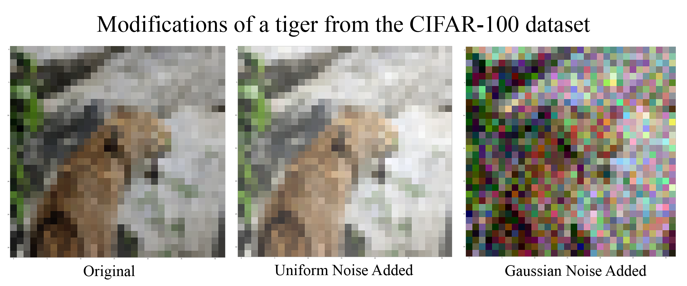
Figure 1. Examples of uniform and Gaussian noise.

2.4. Experimental Setup

We compare the following classification algorithms: k-nearest neighbours (k-NN), logistic regression, support vector machine (SVM), Naive Bayes (NB), decision tree, gradient boosted tree, regular neural network, convolutional neural network (CNN), and pretrained neural network. For the first six, a feature vector was calculated from the images and fed to the models. The feature vector was calculated by using the EfficientNetV2B0 neural network with weights being pre-trained on ImageNet and the output layer removed. In terms of pretrained models, we use VGG-16 as well as ResNet50V2. Their weights were also pretrained on ImageNet.

We train all these algorithms on the aforementioned datasets and we measure fairness by demographic parity, accuracy, FPR, FNR and calibration. The class-specific values of these fairness metrics were calculated and then reduced to a single number. For demographic parity and calibration, this number was simply calculated as the class-specific value subtracted by one. In this way, a value below zero would mean the class was underrepresented in the predictions while a value above zero would mean the class was overrepresented. For the other metrics, the fairness value was calculated to be the value of the metric for that specific class subtracted by the mean of that metric for all the other classes. In this way, a value closer to zero would mean increased fairness. This is written as: $\text{ParityValue}=\text{ClassValue}[t]-\frac{\sum_{i\neq t}\text{ClassValue}[i]}{N_{c}-1}$, where $t$ is the target class and $N_{c}$ is the total number of classes. Therefore, if the target class had an accuracy of 50% and the other classes all had an accuracy of 70% the parity value would be $-20\%$. These values were calculated for data quality of 0.2, 0.4, 0.6, 0.8, and 1.0 for all the data quality variables individually, and for 0.33, 0.66, and 1.0 for all combinations of our data quality measures. Each experiment was repeated three times and results averaged.

3. Results and Discussion

3.1. Fairness with Noisy Labels (RQ1)

Figure 2 shows the level of fairness over training data quality levels across all considered metrics. In the FMNIST dataset for noisy labels, we see that the values for demographic parity, accuracy parity, FPR parity, and calibration were mostly monotonically increasing from less quality to more quality while the FNR parity was mostly monotonically decreasing.

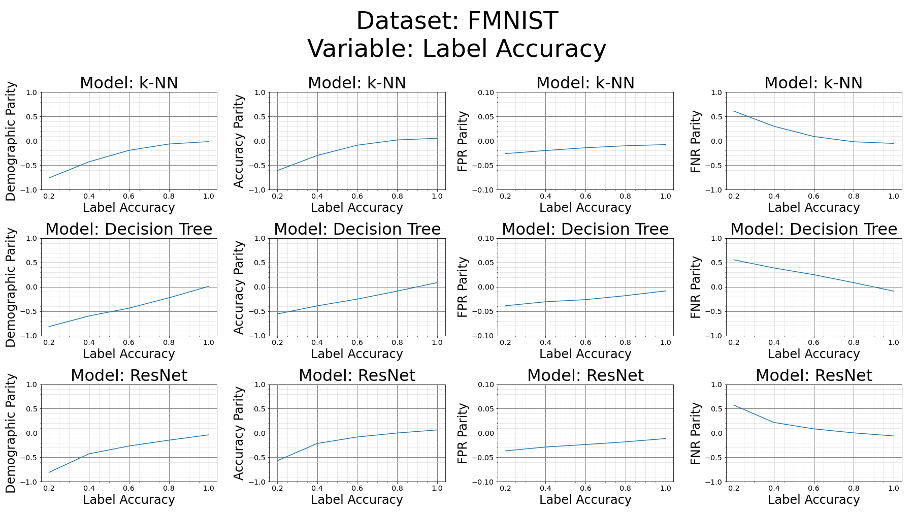
Figure 2. Improvement of fairness over training data quality (i.e., varying levels label noise) on the FMNIST dataset (Note: Some models and measures were omitted due to space constraints).

We observed the same pattern across all of data quality metrics and datasets. This is opposite to our intuition that the quality for a certain class gets worse the false positive rate increases. This can be explained as the quality of a specific class decreases, the model predicts that class a lot less. This implies that ‘fitting to the majority’ seems to be the strongest behaviour we see from these models. Also, Naive Bayes seems to be an outlier in that it is the only model that is resilient to certain types of noise in the data.

We also see that for the domain-specific FMNIST and rice datasets, a low label accuracy is more detrimental to the fairness of the algorithm when measuring equivalence partitioning. For example, a label accuracy of 33% had an accuracy parity value $-59\%$ for SVM meaning that the class that had inaccurate labels was predicted incorrectly 59% worse than every other class. When compared to the same dataset with an equivalence partitioning value of 33%, SVM had an accuracy parity value of $-1\%$. This was observed across all models and all metrics for these datasets and shows that the poor label accuracy was much more detrimental to the results. The results for the rice dataset are shown in Figure 3.

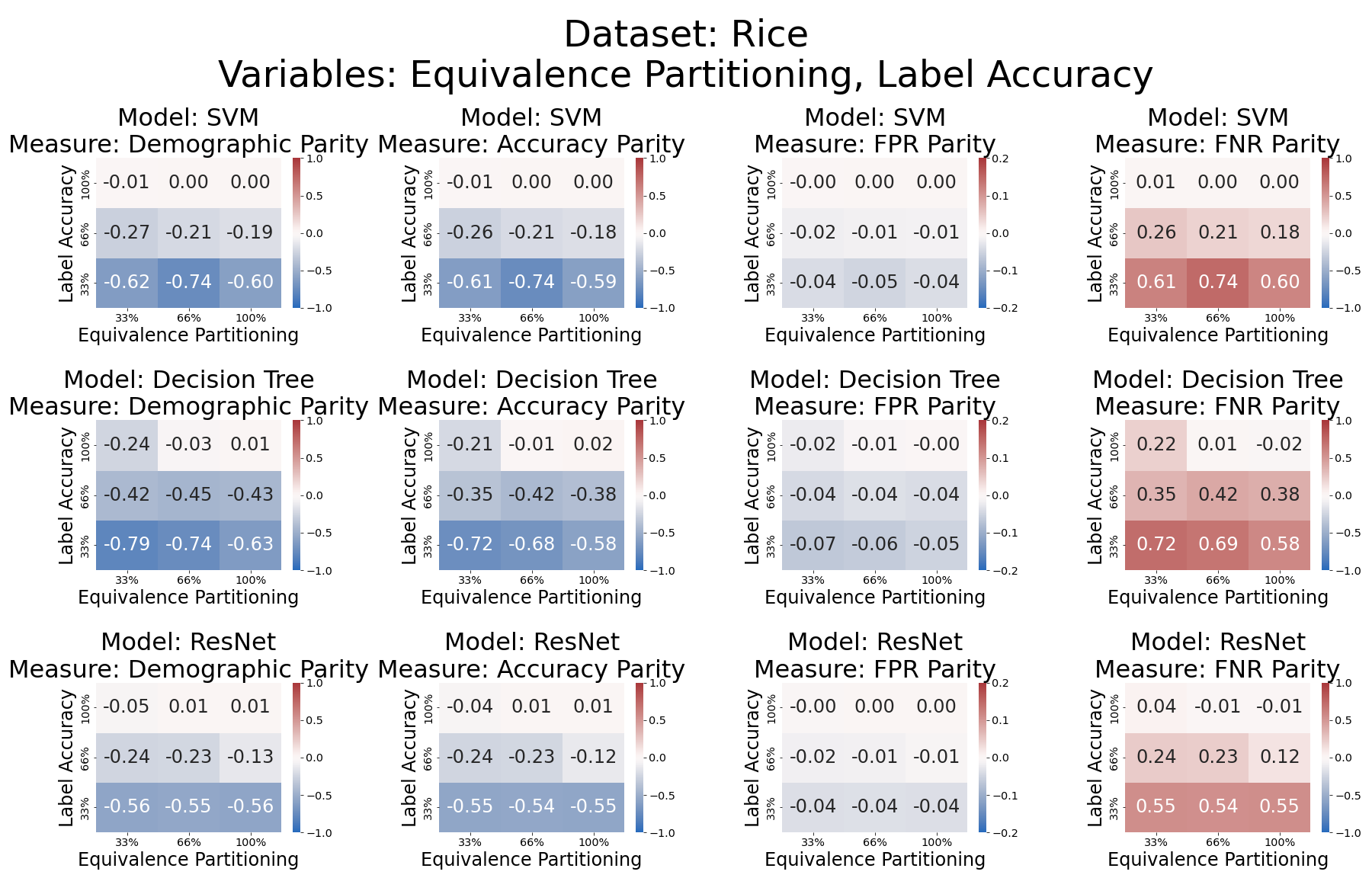
Figure 3. Fairness metrics over training with noisy labels, on the rice dataset.

This effect was less pronounced for the CIFAR-10 and CIFAR-100 datasets where we saw a more symmetrical relation between label accuracy and equivalence partitioning. A possible interpretation is that the models are challenged by the more complex general-domain classification task and so training data quality is much more important for fairness. This is also supported by the non-linear nature in which fairness improves across different equivalence partitioning values in the FMNIST dataset, whereas we see a much more linear trend in the CIFAR-10 and CIFAR-100 datasets. Also, the micro-average $F_{1}$ scores in the CIFAR-10 and CIFAR-100 datasets for the k-NN model are 49.46% and 38.82% respectively while on the FMNIST and rice datasets the same model had $F_{1}$ of 83.42% and 99.2% respectively. Clearly, a change in equivalence partitioning would affect the models built on these datasets a lot less.

3.2. Fairness with Noisy Data (RQ2)

When it comes to noise in data, we saw that the Gaussian noise contributed more to unfairness than uniform noise, even though the values of the brightness of individual pixels in the uniform noise had a greater standard deviation from the original value. This could be attributed to the image-to-feature vector translation which may inherently be more flexible with different brightnesses. Other than that, the results were very similar to what we saw with the equivalence partitioning and label accuracy scenario with most of the unfairness being contributed to by the Gaussian noise rather than the uniform noise even on the more difficult CIFAR datasets. The fairness metrics we considered were all generally extremely correlated when controlling for dataset, model, and data quality metric, except for FNR parity which was negatively correlated.

We found that Naive Bayes (NB) is largely resistant to changes in class balance in the training set (equivalence partitioning), as well as label accuracy. Our explanation is that due to the way in which NB calculates different distributions for each of the classes, the effect of one poor class does not affect the overall model. In the equivalence partitioning case, we can assume that the predicted distribution for the modified class will likely not be that different, and so the outcome for the model would not be significantly affected. In the accuracy modification case, we would see that each of the other classes would have their distributions equally move toward the poor class and so these effects would largely cancel each other out. This interpretation is supported by measuring the overall $F_{1}$ score across different versions of a dataset. For equivalence partitioning values of 0.2, 0.4, 0.6, 0.8, and 1.0, on the CIFAR-100 dataset, we observed $F_{1}$ scores of 47.99%, 47.92%, 48.01%, and 48.04% respectively. For label accuracy values of 0.2, 0.4, 0.6, 0.8, and 1.0, on the CIFAR-100 dataset, we observed $F_{1}$ scores of 47.68%, 47.9%, 47.9%, 47.98%, and 48.04%. The model achieves similar results even with only 20% label accuracy for one of the classes and this is reflected in the almost unchanged values of fairness. The downside of using NB to maximise fairness is that with Gaussian noise NB often displays the worst fairness among all the models we considered.

In terms of algorithms that are most resistant to noise in the data, there was not a clear winner compared to label accuracy and equivalence partitioning. We saw that k-NN, neural network, CNN, as well as both of the transfer learning neural networks seemed to perform well. However, this was not consistent over all of the datasets and the ordering of these algorithms in terms of fairness. In summary, we found that the best algorithm to deal with noise in data and labels varied across datasets and recommend that, if only label accuracy and equivalence partitioning issues exist, Naive Bayes should be used when there is a need to prioritise fairness.

3.3. Transfer Learning and Data Quality (RQ3)

We compare the performance of the transfer learning models and the other neural network models we tested. We found that relative to the regular neural network and convolutional neural network, transfer learning on specialist datasets (FMNIST and rice) showed an average improvement of $-6.5\%$ and $-3.5\%$ respectively in accuracy parity with versions of the dataset with 33% label accuracy and 33% EP values. On the generalist datasets (CIFAR-10 and CIFAR-100) transfer learning had an average improvement of 11.5% and 4.5% respectively. This may due to the complexity of the CIFAR datasets. The transfer learning models are however not significantly better than any other of the models that were tested, in terms of the fairness metrics.

4. Related Work

There is limited research on the direct effect of data quality on fairness. The most related work is that of looking at the effect of data quality on non-class specific metrics such as overall accuracy and $F_{1}$ score (Blake and Mangiameli, 2011; Budach et al., 2022). Other recent work has looked at fairness in ML, as well as at the impact of data quality on ML, unrelated to fairness.

Fairness in Machine Learning. There are a number of solutions to maintain fairness in ML models (Kamiran et al., 2010; Žliobaite et al., 2011; Kearns et al., 2018). These are typically based on the principle of removing (part of) the effect of bias and discrimination in the training data so that the classifiers learnt from this dataset are fair. Previous research has also attempted to describe fairness in algorithms that consist of two steps: (i) defining a set of criteria, and (ii) developing a decision rule to satisfy the criteria (Corbett-Davies et al., 2017). Others have defined their approach by using probability expressions, such as (Feldman et al., 2015; Hardt et al., 2016; Pleiss et al., 2017; Zafar et al., 2017). According to the interviews conducted by Holstein et al. (Holstein et al., 2019), people’s specific needs being sufficiently expressed in ML solutions has raised considerable concerns. This highlights the importance of maintaining a balanced dataset to develop any ML algorithm.

Impact of Data Quality on Machine Learning. Existing research has looked at mitigating bias in ML models. For example, Hube et al. (Hube et al., 2020) proposed a debiasing approach when creating embeddings by incorporating the loss function in the training process with a pre-trained binary (e.g., positive or negative) classifier. Boulitsakis-Logothetis (Boulitsakis-Logothetis, 2022) proposed a modification to the Naive Bayes algorithm that gives guarantees on the statistical parity across protected attributes. This paper found benefits in terms of increases in fairness measures across protected classes but found that accuracy would often be degraded. Bechavod et al. (Bechavod and Ligett, 2017) proposed a method of penalizing unfairness which was inspired by regularization. In this way, they have introduced a data-dependent penalty to the learning process. They found good results balancing between overall accuracy and fairness and performed better than other fairness methods (Zafar et al., 2017). As compared to previous work, we looked at the impact of noisy training data on the level of fairness achieved by models trained with such data, compared the robustness to noise of different models, and also looked at a transfer learning scenario.

5. Conclusions

Our work has addressed questions about the relationship between fairness and data quality. We quantitatively measured fairness across a range of definitions of fairness and data quality. We have made key observations on the relationship between data quality and fairness. We observed the advantage of Naive Bayes in terms of its ability to still give fair results with differing levels of label accuracy as well as equivalence partitioning. We found that Gaussian noise has a much larger impact on fairness on a per standard deviation basis when compared to uniform noise. Finally, we checked if transfer learning had some kind of edge when it came to fairness over both generalist and specialist datasets, and found that they do not.

Acknowledgments. This work is partially supported by the Australian Research Council (ARC) Discovery Project under Grant No. DP190102141, the ARC Training Centre for Information Resilience (Grant No. IC200100022), and the Swiss National Science Foundation (SNSF) under contract number CRSII5_205975.

References

- (1)
- Angwin and Larson (2016) Julia Angwin and Jeff Larson. 2016. Machine bias. ProPublica (May 2016). https://www.propublica.org/article/machine-bias-risk-assessments-in-criminal-sentencing
- Bacham and Zhao (2017) Dinesh Bacham and Janet Zhao. 2017. Machine learning: Challenges, lessons, and opportunities in credit risk modeling. Moody’s Analytics Risk Perspectives IX (Jul 2017). https://www.moodysanalytics.com/risk-perspectives-magazine/managing-disruption/spotlight/machine-learning-challenges-lessons-and-opportunities-in-credit-risk-modeling
- Barocas and Selbst (2016) Solon Barocas and Andrew D. Selbst. 2016. Big Data’s Disparate Impact. California Law Review 104, 3 (2016), 671–732. http://www.jstor.org/stable/24758720
- Bechavod and Ligett (2017) Yahav Bechavod and Katrina Ligett. 2017. Penalizing Unfairness in Binary Classification. https://doi.org/10.48550/ARXIV.1707.00044
- Blake and Mangiameli (2011) Roger Blake and Paul Mangiameli. 2011. The Effects and Interactions of Data Quality and Problem Complexity on Classification. J. Data and Information Quality 2, 2, Article 8 (feb 2011), 28 pages. https://doi.org/10.1145/1891879.1891881
- Boulitsakis-Logothetis (2022) Stelios Boulitsakis-Logothetis. 2022. Fairness-Aware Naive Bayes Classifier for Data with Multiple Sensitive Features. https://doi.org/10.48550/ARXIV.2202.11499
- Budach et al. (2022) Lukas Budach, Moritz Feuerpfeil, Nina Ihde, Andrea Nathansen, Nele Noack, Hendrik Patzlaff, Hazar Harmouch, and Felix Naumann. 2022. The Effects of Data Quality on Machine Learning Performance. In Proceedings of the AAAI 2022 Spring Symposium on Achieving Wellbeing in AI. https://doi.org/10.48550/ARXIV.2207.14529
- Caton and Haas (2020) Simon Caton and Christian Haas. 2020. Fairness in Machine Learning: A Survey. CoRR abs/2010.04053 (2020). arXiv:2010.04053 https://arxiv.org/abs/2010.04053
- Chouldechova (2016) Alexandra Chouldechova. 2016. Fair Prediction with Disparate Impact: A Study of Bias in Recidivism Prediction Instruments. Big Data 5 (10 2016). https://doi.org/10.1089/big.2016.0047
- Chouldechova and Roth (2018) Alexandra Chouldechova and Aaron Roth. 2018. The Frontiers of Fairness in Machine Learning. CoRR abs/1810.08810 (2018). arXiv:1810.08810 http://arxiv.org/abs/1810.08810
- Cinar and Koklu (2019) Ilkay Cinar and Murat Koklu. 2019. Classification of Rice Varieties Using Artificial Intelligence Methods. International Journal of Intelligent Systems and Applications in Engineering 7 (09 2019), 188–194. https://doi.org/10.18201/ijisae.2019355381
- Corbett-Davies and Goel (2018) Sam Corbett-Davies and Sharad Goel. 2018. The Measure and Mismeasure of Fairness: A Critical Review of Fair Machine Learning. CoRR abs/1808.00023 (2018). arXiv:1808.00023 http://arxiv.org/abs/1808.00023
- Corbett-Davies et al. (2017) Sam Corbett-Davies, Emma Pierson, Avi Feller, Sharad Goel, and Aziz Huq. 2017. Algorithmic decision making and the cost of fairness. In Proceedings of the 23rd ACM SIGKDD International Conference on Knowledge Discovery and Data Mining. ACM, 797–806.
- Feldman et al. (2015) Michael Feldman, Sorelle A Friedler, John Moeller, Carlos Scheidegger, and Suresh Venkatasubramanian. 2015. Certifying and removing disparate impact. In Proceedings of the 21th ACM SIGKDD International Conference on Knowledge Discovery and Data Mining. ACM, 259–268.
- Hardt et al. (2016) Moritz Hardt, Eric Price, Nati Srebro, et al. 2016. Equality of opportunity in supervised learning. In Advances in neural information processing systems. 3315–3323.
- Hebert-Johnson et al. (2018) Ursula Hebert-Johnson, Michael Kim, Omer Reingold, and Guy Rothblum. 2018. Multicalibration: Calibration for the (Computationally-Identifiable) Masses. In Proceedings of the 35th International Conference on Machine Learning (Proceedings of Machine Learning Research, Vol. 80), Jennifer Dy and Andreas Krause (Eds.). PMLR, 1939–1948. https://proceedings.mlr.press/v80/hebert-johnson18a.html
- Holstein et al. (2019) Kenneth Holstein, Jennifer Wortman Vaughan, Hal Daumé, III, Miro Dudik, and Hanna Wallach. 2019. Improving Fairness in Machine Learning Systems: What Do Industry Practitioners Need?. In Proceedings of the 2019 CHI Conference on Human Factors in Computing Systems (Glasgow, Scotland Uk) (CHI ’19). ACM, New York, NY, USA, Article 600, 16 pages. https://doi.org/10.1145/3290605.3300830
- Hube et al. (2020) Christoph Hube, Maximilian Idahl, and Besnik Fetahu. 2020. Debiasing Word Embeddings from Sentiment Associations in Names. In Proceedings of the 13th International Conference on Web Search and Data Mining. 259–267.
- Kamiran et al. (2010) Faisal Kamiran, Toon Calders, and Mykola Pechenizkiy. 2010. Discrimination aware decision tree learning. In 2010 IEEE International Conference on Data Mining. IEEE, 869–874.
- Kearns et al. (2018) Michael Kearns, Seth Neel, Aaron Roth, and Zhiwei Steven Wu. 2018. Preventing Fairness Gerrymandering: Auditing and Learning for Subgroup Fairness. In International Conference on Machine Learning. 2569–2577.
- Kleinberg et al. (2017) Jon Kleinberg, Sendhil Mullainathan, and Manish Raghavan. 2017. Inherent Trade-Offs in the Fair Determination of Risk Scores. In 8th Innovations in Theoretical Computer Science Conference (ITCS 2017) (Dagstuhl, Germany, 2017) (Leibniz International Proceedings in Informatics (LIPIcs), Vol. 67), Christos H. Papadimitriou (Ed.). Schloss Dagstuhl–Leibniz-Zentrum fuer Informatik, 43:1–43:23. https://doi.org/10.4230/LIPIcs.ITCS.2017.43
- Kohavi and Provost (1998) Ron Kohavi and Foster Provost. 1998. Glossary of terms. https://ai.stanford.edu/~ronnyk/glossary.html
- Mani et al. (2019) Senthil Mani, Anush Sankaran, Srikanth Tamilselvam, and Akshay Sethi. 2019. Coverage Testing of Deep Learning Models using Dataset Characterization. CoRR abs/1911.07309 (2019). arXiv:1911.07309 http://arxiv.org/abs/1911.07309
- Nair et al. (2019) Nimisha G Nair, Pallavi Satpathy, Jabez Christopher, et al. 2019. Covariate shift: A review and analysis on classifiers. In 2019 Global Conference for Advancement in Technology (GCAT). IEEE, 1–6.
- Pleiss et al. (2017) Geoff Pleiss, Manish Raghavan, Felix Wu, Jon Kleinberg, and Kilian Q Weinberger. 2017. On fairness and calibration. In Advances in Neural Information Processing Systems. 5680–5689.
- Sweeney (2013) Latanya Sweeney. 2013. Discrimination in Online Ad Delivery: Google Ads, Black Names and White Names, Racial Discrimination, and Click Advertising. Queue 11, 3 (mar 2013), 10–29. https://doi.org/10.1145/2460276.2460278
- Zafar et al. (2017) Muhammad Bilal Zafar, Isabel Valera, Manuel Gomez Rodriguez, and Krishna P Gummadi. 2017. Fairness beyond disparate treatment & disparate impact: Learning classification without disparate mistreatment. In Proceedings of the 26th International Conference on World Wide Web. International World Wide Web Conferences Steering Committee, 1171–1180.
- Žliobaite et al. (2011) Indre Žliobaite, Faisal Kamiran, and Toon Calders. 2011. Handling conditional discrimination. In 2011 IEEE 11th International Conference on Data Mining. IEEE, 992–1001.