Spiking Neural Networks in the Alexiewicz Topology: A New Perspective on Analysis and Error Bounds

Abstract

In order to ease the analysis of error propagation in neuromorphic computing and to get a better understanding of spiking neural networks (SNN), we address the problem of mathematical analysis of SNNs as endomorphisms that map spike trains to spike trains. A central question is the adequate structure for a space of spike trains and its implication for the design of error measurements of SNNs including time delay, threshold deviations, and the design of the reinitialization mode of the leaky-integrate-and-fire (LIF) neuron model. First we identify the underlying topology by analyzing the closure of all sub-threshold signals of a LIF model. For zero leakage this approach yields the Alexiewicz topology, which we adopt to LIF neurons with arbitrary positive leakage. As a result LIF can be understood as spike train quantization in the corresponding norm. This way we obtain various error bounds and inequalities such as a quasi isometry relation between incoming and outgoing spike trains. Another result is a Lipschitz-style global upper bound for the error propagation and a related resonance-type phenomenon.

Keywords Leaky-Integrate-and-Fire (LIF) Neuron  $\cdot$ Spiking Neural Networks (SNN)  $\cdot$ Re-Initialization  $\cdot$ Quantization  $\cdot$ Error Propagation  $\cdot$ Alexiewicz Norm

1 Introduction

Spiking neural networks (SNNs) are artificial neural networks of interconnected neurons that asynchronously process and transmit spatial-temporal information based on the occurrence of spikes that come from spatially distributed sensory input neurons. The most commonly used neuron model in SNNs is the leaky-integrate-and-fire (LIF) model Gerstner et al. (2014). Despite its strong simplification of the biological way of spike generation, the LIF model has proven useful in particular when modeling the temporal spiking characteristics in the biological nervous system. For an overview see, e.g., Tavanaei et al. (2019); Nunes et al. (2022). At the interfaces, that is from real-world to SNN, and from SNN output to real-world, in general there is the need to translate analogue perceived intensities into spike trains, and later on, after processing, to decode the resulting spike trains into meaningful decisions. Some approaches prefer a rate-based encoding while others emphasize on the timing, e.g., of first arriving spikes Guo et al. (2021). In the context of sampling time-varying signals also alternatives of LIF are encountered to sample real analogue signals into spikes, e.g., by delta coding or synonymously used terms like send-on-delta, level crossing or threshold-based sampling Miskowicz (2006); Liu et al. (2014); Yousefzadeh and Sifalakis (2022).

Due to their particular nature of asynchronous and sparse information processing, SNNs are studied mainly for two reasons: first, as a simplified mathematical model in the context of computational neuroscience aiming at a better understanding of biological neural circuits, and second, as a further step towards more powerful but energy-efficient embedded AI edge solutions to process time-varying signals with a wide range of applications including visual processing Amir et al. (2017); Yousefzadeh and Sifalakis (2022), audio recognition Wu et al. (2018), speech recognition Wu et al. (2020), biomedical signal processing Hassan et al. (2018) and robotic control Kabilan and Muthukumaran (2021); Yamazaki et al. (2022). New application scenarios are emerging in the context of edge AI and federated learning across a physically distributed network of resource-constrained edge devices to collaboratively train a global model while preserving privacy Yang et al. (2022). Of particular interest are applications in the emerging field of brain-computer interfaces which opens up new perspectives for the treatment of neurological diseases such as Parkinson’s disease Dethier et al. (2013); Gege et al. (2021). For an overview on the performance comparison between SNNs and conventional vector-based artificial neural networks see Deng et al. (2020). However, the full potential of SNNs, in particular their energy efficiency and dynamic properties, will only become manifest when implemented on dedicated neuromorphic hardware, leading to ongoing research in this direction Bouvier et al. (2019); DeBole et al. (2019); Ostrau et al. (2022); Michaelis et al. (2022).

However, despite the great potential of SNNs and the ongoing research efforts the practical realizations are few so far. To this end, the research on SNNs is still in an early phase of maturity, particularly lacking mathematical foundation which becomes necessary due to the special hybrid continuous-discrete nature of SNNs and the underlying paradigm shift towards event-based signal processing.

A closer look at the different ways of sampling makes apparent this paradigm shift as sketched in Fig. 1. In equidistant-based uniform sampling, the mathematics of information encoding and processing is based on regular Dirac combs and its embedding in Hilbert spaces with its powerful mathematical tools of convolution, orthogonal projection, and based thereupon spectral analysis, signal filtering and reconstruction. As sequences of uniformly distributed Dirac pulses in time, regular Dirac combs and related concepts of signal decomposition into regular wave forms can be viewed as a trick that allows time to be treated mathematically as a space variable. However, this mathematical abstraction neglects the time information that is implicitly encoded by events Miskowicz (2006). To this end, the resulting mathematics of uniform sampling and signal processing becomes basically vector-based. In contrast, in biological information processing systems and bio-inspired neuromorphic computing, see e.g., Tavanaei et al. (2019),  Nunes et al. (2022), the paradigm of information encoding somewhat flips the role of regularity w.r.t time versus amplitude. While in uniform sampling and related signal processing time is treated as a regular structure and the amplitudes of sampled values are kept flexible, in bio-inspired sampling and signal processing the amplitudes are forced into a regular structure by means of thresholding while keeping the handling of time flexible.

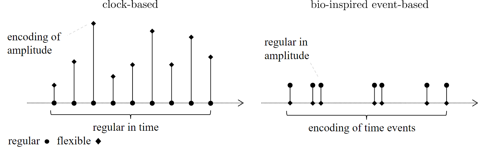
Figure 1: Paradigm shift in information encoding of uniform (left) versus threshold-based (right) sampling.

This paradigm shift of information encoding will have implications on the mathematical foundation of handling irregularity in time, that is to handle sequences of Dirac impulses beyond a regular comb structure, see Figure 1.

While regular time leads to Hilbert spaces, and inherently to the Euclidean norm, our approach is to revise the Euclidean view of geometry in this context in favor of an approach based on alternative metrics which become necessary if we postulate certain analytical properties on the topological and metric structure of the space of spike trains in combination with neuronal models and spiking neural networks as used in neuromorphic computing. Our paper is a contribution to the mathematical foundation of SNNs by elaborating on postulates on the topology of the vector space of spike trains in terms of sequences of weighted Dirac impulses. Our approach is a follow-up of Moser and Natschläger (2014); Moser (2015, 2016, 2017); Moser and Lunglmayr (2019) which discusses the discrepancy measure as a special range-based metric for spike trains for which a quasi-isometry relation for threshold-based sampling between analog signals as input and spike trains as output of a leaky-integrate-and-fire neuron can be established. In this paper, we go beyond sampling and show that range-based metrics also play a special role for the mathematical conception of error, resp., deviation analysis based on spike trains, and thus for understanding, analyzing, and bounding error propagation of spiking neural networks (SNNs).

The paper is structured as follows. In Section 2, we fix notation and prepare preliminaries from SNNs based on leaky integrate-and-fire neuron model and the mathematical idealized assumption of instantaneous realization of events due to an impulse input. In this context, we discuss proposed variants of re-initialization after the firing event and revise the re-initialization mode known as reset-by-subtraction in the general setting of spike amplitudes that exceed multiples of the threshold. Such high spike amplitudes can arise in SNNs by scaling the input channels by weights. This way we introduce the reset-to-mod re-initialization which results actually from a consequent application of the assumption of instantaneous events to reset-by-subtraction. The resulting operation can be considered as modulo division. reset-to-mod allows to take a broader view on the mathematics of LIF as endomorphism that operates on the vector space of spike trains of weighted Dirac impulses. This way we study the resulting LIF operator, specify the above motivated postulates in Section 3 and derive a solution based on a topological argument in Subsection 3.1, leading to the Alexiewicz norm for integrate-and-fire (IF). We generalize this norm for leaky integrate-and-fire (LIF) and, as a main result, we show in Subsection 3.2 that the LIF operator acts as spike quantization in the grid given by the corresponding norm. The related inequality turns out to be useful when it comes to the analysis of error and signal propagation due to perturbations or added spikes in the input channels. Section 4 focuses on the effect of added spikes in the input channel, which results in a Lipschitz-style upper bound for the LIF model and feed-forward SNNs in general. This analysis also shows that there can be a principle change in the input-output characteristic along the transition from integrate-and-fire with zero leakage to arbitrarily small leaky parameters. Section 5 reports on simulations that illustrate our theoretical approach.

2 Preliminaries

First we recall the LIF neural model with its computational variants and fix notation. It has a long history which goes back to Lapicque (1907). For an overview on its motivation and relevance in neuroscience and neuromorphic computing see Gerstner et al. (2014),  Dayan and Abbott (2001) and Eshraghian et al. (2021). Situated in the middle ground between biological plausibility and technical feasibility, the LIF model abstracts away the shape and profile of the output spike. This way spikes are mathematically represented as Dirac delta impulses.

Therefore, we start with spike trains as input signals which we assume to be given mathematically as sequences of weighted Dirac impulses, i.e.,

$$\eta(t):=([a_{i};t_{i}]_{i})(t):=\sum_{i\in\mathbb{N}_{0}}a_{i}\,\delta_{t_{i}}(t),$$ (1)

where $a_{i}\in\mathbb{R}$ and $\delta_{t_{i}}$ refers to a Dirac impulse shifted by $t_{i}$. $\mathbb{N}_{0}$ means that there is no bound for the number of spikes, though for convenience we assume that for each spike train the number is finite. For convenience and without loss of generality, to ease notation below we assume that $t_{0}=0$ and $a_{0}=0$. The empty spike train is denoted by $\emptyset$.

$(\mathbb{S},+,\cdot)$ denotes the vector space of all spike trains (1) based on usual addition and scaling, which later on will be equipped with a metric $d(.,.)$, resp. norm $\|.\|$, to obtain the metric space $(\mathbb{S},d)$, respectively, normed space $(\mathbb{S},d)$.

Mathematically, the LIF neuron model is actually an endomorphism, $\mbox{LIF}_{\vartheta,\alpha}:\mathbb{S}\rightarrow\mathbb{S}$, that is determined by two parameters, the threshold $\vartheta>0$ and the leaky time constant $\alpha>0$ and the mode for resetting the neuron after firing, respectively, the charging/discharging event. In this paper we consider three reset modes, reset-to-zero, reset-by-subtraction and reset-to-mod. According to Eshraghian et al. (2021), reset-to-zero means that the potential is reinitialized to zero after firing, while reset-by-subtraction subtracts the $\vartheta$-potential $u_{\vartheta}$ from the membrane’s potential that triggers the firing event. As a third variant we use the term reset-to-mod, which can be understood as instantaneously cascaded application of reset-by-subtraction according to the factor by which the membrane’s potential exceeds the threshold which results in a modulo computation. This means, in the reset-to-mod case the re-initialization starts with the residue after subtracting the integral multiple of the threshold from the membrane’s potential at firing time.

Setting $t_{0}^{(1)}:=0$ (where the upper index indicates the layer, here the output of LIF) and $\eta_{in}(t):=([a_{i};t_{i}^{(0)}]_{i})(t)$ the mapping

$$\sum_{i\in\mathbb{N}_{0}}b_{i}\,\delta_{t_{i}^{(1)}}=\eta_{out}=\mbox{LIF}_{\vartheta,\alpha}(\eta_{in})$$

is recursively given by

$$t_{i+1}^{(1)}=\inf\left\{t\geq t_{i}^{(1)}:\,\left|u_{\vartheta,\alpha}(t_{i}^{(1)},t)\right|\geq\vartheta\right\},$$ (2)

where

$$u_{\alpha}(t_{i},t):=\int^{t}_{t_{i}}e^{-\alpha(\tau-t_{i})}\left(\eta_{in}(\tau)-\mbox{discharge}(t_{i},\tau)\right)d\tau$$ (3)

models the dynamic change of the neuron membrane’s potential after an input spike event at time $t_{i}$ (based on the assumption of instantaneous increase, resp. decrease). At the moment when the absolute value of the membrane potential touches the threshold-level, $\vartheta>0$, an output spike is generated whose amplitude is given by $b_{i+1}=+\vartheta$ or $=-\vartheta$ depending on whether the membrane’s potential $u_{\alpha}$ in (2) is positive or negative.

The process of triggering an output spike is actually a charge-discharge event that is followed by the re-initialization of the membrane’s potential modeled by an instantaneously acting discharge process

$$\mbox{discharge}(t_{i}^{(1)},\tau):=\left\{\begin{array}[2]{lcl}u_{i}\,\delta_{t_{i}^{(1)}}(\tau)&\ldots&\mbox{for {\it reset-to-zero}},\\ \mbox{sgn}(u_{i})\,\vartheta\,\delta_{t_{i}^{(1)}}(\tau)&\ldots&\mbox{for {\it reset-by-subtraction}},\\ \mbox{sgn}(u_{i})[u_{i}/\vartheta]\,\vartheta\,\delta_{t_{i}^{(1)}}(\tau)&\ldots&\mbox{for {\it reset-to-mod}},\end{array}\right.$$ (4)

where $u_{i}:=u_{\alpha}(t_{i-1},t_{i})$, $\mbox{sgn}(x)\in\{-1,0,1\}$ is the signum function and

$$[x]:=\mbox{sgn}(x)\max\{k\in\mathbb{Z}:k\leq|x|\}$$ (5)

realizes integer quantization by truncation.

The integration in (2) models the voltage in an RC circuit as response to current impulses. Note that the immediate reset without delay in (2) is an idealization from biology or hardware realizations. Anyway, since in practical realizations spikes are sparse in time (or should be) this idealization is a justifiable approximation. reset-to-zero and reset-by-subtraction can show quite different behavior if the spike amplitudes are large.

The reset-by-subtraction mode can be understood as compensation event so that the net voltage balance of the spiking event equals zero, i.e. in case of an output spike with amplitude $\vartheta$ the membrane is actually discharged by this amount. Accordingly, though not always made clear in the literature, see for example Eshraghian et al. (2021), this assumption has the subtle consequence that an increase of the membrane potential $u$ by multiples $[u/\vartheta]$ of the threshold level $\vartheta$ results in a discharge of the membrane’s potential by the same amount, i.e., $[u/\vartheta]\vartheta$.

This can also be seen virtually as sequence of $[u/\vartheta]$-many $\vartheta$-discharge actions, which acting in sequence in instantaneous time produce the same result, that is an output spike with amplitude $[u/\vartheta]\vartheta$. Here we express the amplitude of the output spikes as multiple of the unit in terms of the threshold potential $\vartheta$. For example, consider a single spike $\eta_{in}(t):=a_{1}\delta_{t_{1}}(t)$ with large amplitude $|a_{1}|>\vartheta$. Note that due to the idealization of instantaneous actions of charge and discharge events the discharge model in the reset-by-subtraction mode implies that $\eta_{in}=a_{1}\delta_{t_{1}}$ is mapped to

$$b_{1}\delta_{t_{1}}=\mbox{LIF}_{\vartheta,\alpha}(a_{1}\delta_{t_{1}}),\,\,\,b_{1}=[a_{1}/\vartheta]\,\vartheta.$$ (6)

Fig. 2 illustrates LIF with reset-by-subtraction.

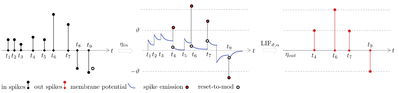
Figure 2: LIF in continuous time with reset-by-subtraction, resp. reset-to-mod; at $t_{6}$ the amplitude $a_{6}\in(2\vartheta,3\vartheta)$ of the input spike, which causes a two times cascaded reset-by-subtraction resulting in an output spike amplitude $b_{6}=2\vartheta=[a_{6}/\vartheta]\,\vartheta$.

Depending on the research and application context, discrete approximations of the LIF model (2) become popular, particularly to simplify computation and to make the application of deep learning methods to spike trains easier Eshraghian et al. (2021). Under the assumptions

• continuous time $t\in[0,\infty)$ is replaced by discrete time $n\Delta t\in\Delta t\,\mathbb{N}_{0}$, where $\Delta t\ll\alpha$;

• instantaneous increase, respectively decrease of the membrane’s potential (3);

we obtain a discrete computational model, where the input signal $\eta_{in}=\sum_{i}a_{i}\delta_{t_{i}}$ in continuous time is replaced by the sequence

$$\hat{a}_{k}:=\left\{\begin{array}[pos]{lcl}a_{i}&&k=[t_{i}/\Delta t],\\ 0&&\mbox{else}\\ \end{array}\right.$$ (7)

which is well-defined if $\Delta t$ is chosen sufficiently small so that at most one Dirac impulse hits a time interval $I_{k}=[k\Delta t,(k+1)\Delta t)$. The amplitudes $\hat{b}_{n}$, $n=0,1,\ldots$, of the output spike train are defined as for continuous time. This way, finally we get the discrete LIF model, $\widehat{\mbox{LIF}}_{\vartheta,\beta,\Delta t}:\mathbb{R}^{\mathbb{N}_{0}}\rightarrow\mathbb{R}^{\mathbb{N}_{0}}$, $(\hat{b}_{k})_{k}=\widehat{\mbox{LIF}}_{\vartheta,\beta,\Delta t}((\hat{a}_{k})_{k})$, as outlined in Algorithm 1.

Algorithm 1 Simplified Discrete LIF model $\widehat{\mbox{LIF}}_{\vartheta,\beta,\Delta t}$

Step 0: Initialization: $\hat{a}=(\hat{a}_{k})_{k}$, $u_{0}:=0$, $\hat{b}_{0}=0$, $\beta:=(1-\frac{\Delta t}{\alpha})$;
Step 1: Update Membrane Potential: $u_{n+1}:=\beta\,u_{n}+\hat{a}_{n}-\hat{b}_{n}$
Step 2: Check Threshold: Update time $n\mapsto n+1$ and check whether $|u_{n}|\geq\vartheta$. If ’no’, then set $\hat{b}_{n}:=0$ and repeat Step 1; if ’yes’ then output a spike at time step with amplitude $u_{n}$ and move on to Step 3.
Step 3: Discharge Event: According to the re-initialization mode set

$$\hat{b}_{n}:=\left\{\begin{array}[2]{lcl}u_{n}&\ldots&\mbox{for {\it reset-to-zero}},\\ \mbox{sgn}(u_{n})\vartheta&\ldots&\mbox{for {\it reset-by-subtraction}},\\ {\left[u_{n}/\vartheta\right]}\vartheta&\ldots&\mbox{for {\it reset-to-mod}}.\end{array}\right.$$ (8)

Step 4: Repeat steps Steps 1,2,3 until all input spikes are processed.

With this mathematical clarification of the LIF model, in continuous and discrete time, we are in the position to study integrate-and-fire as spike quantization and provide upper bounds for the quantization error in Section 3.2.

In this paper we consider feed-forward spiking neural networks, $\mbox{SNN}:\mathbb{S}^{N_{0}}\rightarrow\mathbb{S}^{N_{L}}$ which are mappings given by weighted directed acyclic graphs $(V,E)$ connecting LIF units with fixed parameters $\vartheta$ and $\alpha$. SNN takes $N_{0}$ spike trains as input and maps them to $N_{L}$ output spike trains. The underlying graph can be arranged in hierarchies starting from the first layer $1$ up to layer $L$. We enumerate the LIF nodes in the $k$th layer by $(k,i_{k})$, where $i_{k}\in\{1,\ldots,N_{k}\}$.

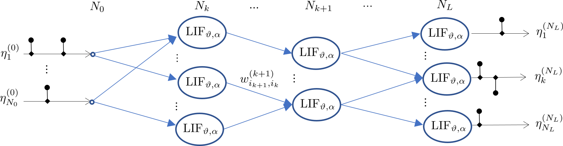
Figure 3: SNN as weighted directed acyclic graph.

For convenience we consider the input spike trains as $0$ layer. The weight $w^{(k+1)}_{i_{k+1},i_{k}}$ of an edge $[(k,i_{k}),(k+1,i_{k+1})]\in E$ connecting the $i_{k}$-th neuron in the $k$-th layer with the $i_{k+1}$-th neuron in the $(k+1)$-th layer rescales accordingly the weights of the spike train being transmitted from the former neuron to the latter. See Fig. 3 for an illustration. This way the mapping SNN can be represented by the tuple of weight matrices $W=[W^{(1)},\ldots,W^{(N_{L})}]$, where

SNN $$= [W^{(1)},\ldots,W^{(N_{L})}],$$ (9)

$$W^{(k+1)} = (w^{(k+1)}_{i_{k+1},i_{k}})\in\mathbb{R}^{N_{k+1}\times N_{k}}.$$

3 Which Topology for the Space of Spike Trains is Appropriate?

Our approach starts with two main postulates a topology for spike trains should satisfy, see Fig. 4:

Postulate 1: Two spike trains that differ only by small delays of their spikes or small additive noise should be considered close where the notion of closeness should not depend on the number of spikes. Postulate 2: Small perturbations in the system’s configuration parameters should end up in similar input-output behavior, e.g., if the threshold deviates only by some small value.

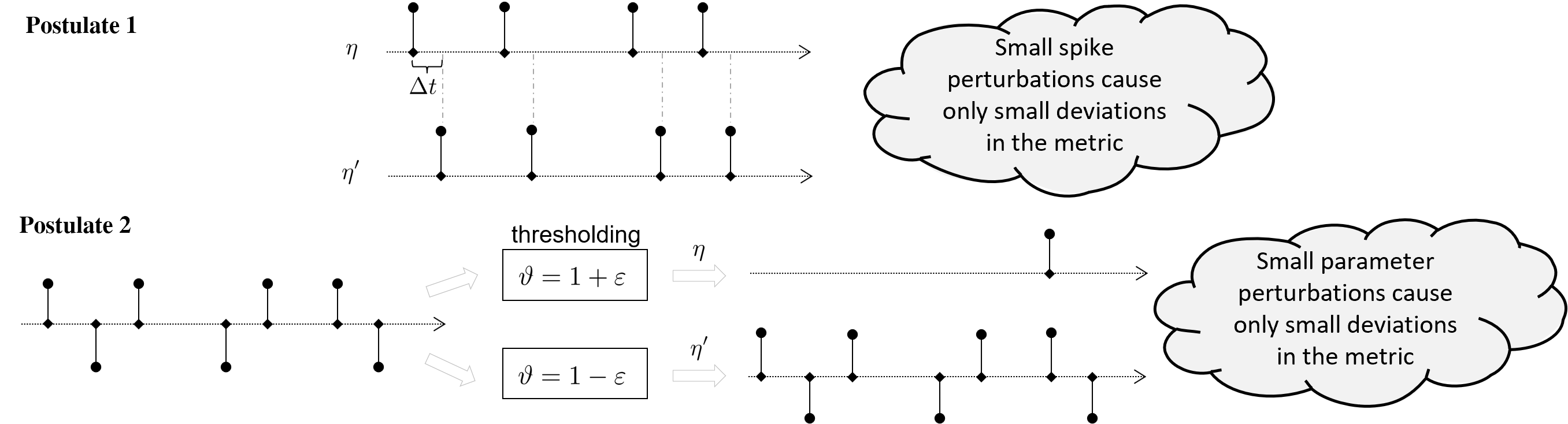
Figure 4: Postulates for an adequate metric $d(.,.)$ for spike strains.

Note that the widely spread Euclidean approach based on summing up squared differences does not meet these postulates. For example, in the context of back propagation expressions of the type $d_{E}(\eta,\eta^{\prime})^{2}:=\sum_{i}(t_{i}-t_{i}^{\prime})^{2}$ are used, see, e.g. Bohte et al. (2000). Apart from the problem that this definition is only well defined if there is a one-to-one correspondence between the spikes in the first and the second spike train. This ansatz may be useful for certain algorithms in a certain setting, but due to the lack of well-definedness it is not suitable for an axiomatic foundation of a generally valid theory. For example, this ansatz is not well-defined in the scenario of Postulate 2 if the first spike train is empty and the second not. Also Postulate 1 is problematic as the error depends on the number of spikes. A large error can result from a large delay of a single spike or of many small delays. See also Moser and Natschläger (2014); Moser (2015). In addition, the sign of the spike is not taken into account.

3.1 Alexiewicz Topology

In order to get an idea about signals that should be considered close in the topology let us consider the set $C$ of all sub-threshold input spike trains to a LIF neuron $\mbox{LIF}_{\vartheta,\alpha}:\mathbb{S}\rightarrow\mathbb{S}$. Note that $C$ is the pre-image of LIF of the empty spike trains, i.e., $C:=\mbox{LIF}_{\vartheta,\alpha}^{(-1)}(\{\emptyset)\}$. $C$ is obviously not a closed set, as, e.g., all spike trains $\eta_{k}:=(\vartheta-1/k)\delta_{t_{1}}$ are below threshold but not its pointwise limit. Taking also all limits into account we obtain a notion of closure $\overline{C}$ of $C$. $\overline{C}$ can be characterized in the following way, see A.

Lemma 1

For a leaky integrate-and-fire neuron $\mbox{LIF}_{\vartheta,\alpha}:\mathbb{S}\rightarrow\mathbb{S}$ with $0\leq\alpha<\infty$ we have:

$$\eta=\sum_{i}a_{i}\delta_{t_{i}}\in\overline{\mbox{LIF}_{\vartheta,\alpha}^{(-1)}(\{\emptyset)\}}\Longleftrightarrow\max_{n}\left|\sum_{i=1}^{n}a_{i}e^{-\alpha(t_{n}-t_{i})}\right|\leq\vartheta.$$

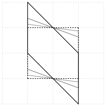
Figure 5: $\|.\|_{A,\alpha}$-unit balls for spike trains $\eta=a_{1}\delta_{0}+a_{2}\delta_{1}$ for $\|.\|_{A,\alpha}$ with $\alpha=0$ (solid black), $\alpha=\infty$ (dashed), $\alpha=1$ and $\alpha=2$ (gray)

Note that

$$\|([a_{i};t_{i}])_{i}\|_{A,\alpha}:=\max_{n}\left|\sum_{j=1}^{n}a_{j}e^{-\alpha(t_{n}-t_{j})}\right|$$ (10)

defines a norm on the vector space $\mathbb{S}$, which justifies the $\|.\|$ notation. As immediate consequences from the definition (10) we obtain

$$\|\eta\|_{A,\alpha}=\inf\left\{\vartheta>0:\mbox{LIF}_{\vartheta,\alpha}(\eta)=\emptyset\right\},$$ (11)

and

$$\forall\alpha,\beta\in(0,\infty),\eta\in\mathbb{S}:\|\mbox{LIF}_{\vartheta,\alpha}(\eta(\cdot))\|_{A,\alpha}=\|\mbox{LIF}_{\vartheta,\beta}\left(\eta(\alpha/\beta\,\cdot)\right)\|_{A,\beta}.$$ (12)

This way, $\overline{\mbox{LIF}_{\vartheta,\alpha}^{(-1)}(\{\emptyset)\}}$ turns out to be the ball $B_{A,\alpha}(\vartheta)$ centered at $\emptyset$ of radius $\vartheta$ w.r.t the norm $\|.\|_{A,\alpha}$. For $\alpha=0$ the length of the time intervals between the events do not have any effect, and we get the norm $\|(a_{i})_{i}\|_{A,0}=\max_{n}\left|\sum_{i=1}^{n}a_{i}\right|$. By looking at $a_{i}$ as width of a step of a walk up and down along a line, $\|.\|_{A,0}$ marks the maximum absolute route amplitude of the walk.

Range measures are studied in the field of random walks in terms of an asymptotic distribution resulting from diffusion process Finch (2018); Jain and Orey (1968). A similar concept is given in terms of the diameter $\|(a_{i})_{i}\|_{D}$ of a walk, i.e., $\|(a_{i})_{i}\|_{D}:=\max_{1\leq m\leq n\leq N}\left|\sum_{i=m}^{n}a_{i}\right|$, which immediately can be generalized to $\|(a_{i})_{i}\|_{D,\alpha}:=\max_{1\leq m\leq n\leq N}|\sum_{j=m}^{n}a_{j}e^{-\alpha(t_{n}-t_{j})}|$. Note that $\|(a_{i})_{i}\|_{A,\alpha}\leq\|(a_{i})_{i}\|_{D,\alpha}\leq 2\|(a_{i})_{i}\|_{A,\alpha}$ stating the norm-equivalence of $\|.\|_{A,\alpha}$ and $\|.\|_{D,\alpha}$.

While the unit ball $B_{A,0}$ w.r.t $\|.\|_{A,0}$ can be understood by shearing the hypercube $[-1,1]^{N}$, see B, the geometric characterization of the related unit ball $B_{D,0}$ of $\|.\|_{D,0}$ is more tricky, see Moser (2012).

For an illustration of the corresponding unit balls for two spikes (2D case) see Fig. 5.

These concepts are related to the more general concept of discrepancy measure, see Chazelle (2000); Moser (2011), which goes back to Hermann Weyl Weyl (1916) and is defined on the basis of a family $\mathcal{F}$ of subsets $F$ of the universe of discourse, i.e., $\mu((a_{i})_{i})=\sup_{F\in\mathcal{F}}|\sum_{i\in F}a_{i}|$. For $\|.\|_{A}$ the family $\mathcal{F}$ consists of all index intervals $\{0,\ldots,m\}$, while for $\|.\|_{D}$ the family $\mathcal{F}$ consists of all partial intervals $\{m,\ldots,n\}$, $m,n\in\{1,\ldots,N\}$. Therefore we refer particularly to $\|.\|_{A}$, resp. $\|.\|_{D}$, as example of a discrepancy measure.

An analogous concept, $\|f\|:=\sup_{[a,b]}|\int_{[a,b]}fd\mu|$, can be defined for functions $f$ and tempered distributions such as Dirac delta impulses by using integrals instead of the discrete sum, which is known in the literature as Alexiewicz semi-norm Alexiewicz (1948). As spike trains live in continuous time, in the end our topology we are looking for is the Alexiewicz topology, which meets the postulates above. However, most of the reasoning and proofs in the context of this paper can be boiled down to discrete sequences, hence utilizing the discrepancy norm.

3.2 Spike Train Quantization

Interestingly, as pointed out by Moser and Lunglmayr (2023), LIF can be understood as a $\|.\|_{A,\alpha}$-quantization operator satisfying

$$\|\mbox{LIF}_{\vartheta,\alpha}(\eta)-\eta\|_{A,\alpha}<\vartheta.$$ (13)

Moser and Lunglmayr (2023) provides a proof of (13) for weighted Dirac impulses as input signal to the LIF, see C. Here, first we note that (5) also applies to the discrete version of Algorithm 1. The proof is analogous. Second, we state a generalization to piecewise continuous functions. This way, we show that LIF acts like a signal-to-spike-train quantization. The generalization of Dirac pulses to more general classes of signals is especially important for a unifying theory that combines analog spike sampling and SNN-based spike-based signal processing. An extension to the general class of locally integrable functions is also possible but requires the introduction of the Henstock-Kurzweil integral Kurtz and Swartz (2004), which is postponed to future research.

Theorem 1

(13) also holds for piecewise continuous functions $\eta$, i.e., functions having at most a finite number of discontinuities.

Proof.

The idea is to construct a $\hat{\eta}=\sum_{i}a_{i}\delta_{t_{i}}\in\mathbb{S}$ such that $\int_{t_{0}}^{t_{i}}\hat{\eta}(t)e^{\alpha t}dt=\int_{t_{0}}^{t_{i}}\eta(t)e^{\alpha t}dt$ for all $t_{i}$. This can be achieved by utilizing the mean value theorem for integrals. First, partition the time domain into intervals $U_{k}=(u_{k-1},u_{k})$ on which $\eta$ is continuous. On $U_{k}$, the mean value theorem guarantees the existence of $s_{k}\in U_{k}$ such that $\int_{U_{k}}\eta(t)e^{\alpha t}dt=|U_{k}|\eta(s_{k})e^{\alpha s_{k}}$. Then define the sequence $(t_{i})_{i}$ consisting of all $s_{k}$ and the $u_{k}$. For $t_{i}=s_{k}$ define $a_{i}:=|U_{k}|\eta(s_{k})$ and for $t_{i}=u_{k}$ define $a_{i}:=\lim_{\varepsilon\rightarrow 0}\int_{u_{k}-\varepsilon}^{u_{k}+\varepsilon}\eta dt$. Refine this partition so that also the time points $t_{i}^{*}$ of the output spikes of $\mbox{LIF}_{\vartheta,\alpha}(\eta)=\sum_{i}b_{i}\delta_{t_{i}^{*}}$ are taking into account as border points of the $U_{i}$ intervals. This way we obtain for all $t_{i}$:

$$\int_{t_{0}}^{t_{i}}\eta(t)e^{-\alpha(t_{i}-t)}dt=\int_{t_{0}}^{t_{i}}\hat{\eta}(t)e^{-\alpha(t_{i}-t)}dt.$$ (14)

Moreover, since all time points $t_{i}^{*}$ are contained in $(t_{i})_{i}$, we also have

$$\mbox{LIF}_{\vartheta,\alpha}(\eta)=\mbox{LIF}_{\vartheta,\alpha}(\hat{\eta}).$$ (15)

Putting (14) and (15) together closes the proof. $\square$

Fig. 6 illustrates the quantization for different values of $\alpha$ w.r.t $\|.\|_{A,\alpha}$. Note that for $\alpha\rightarrow\infty$ we obtain the standard $\|.\|_{\infty}$-quantization.

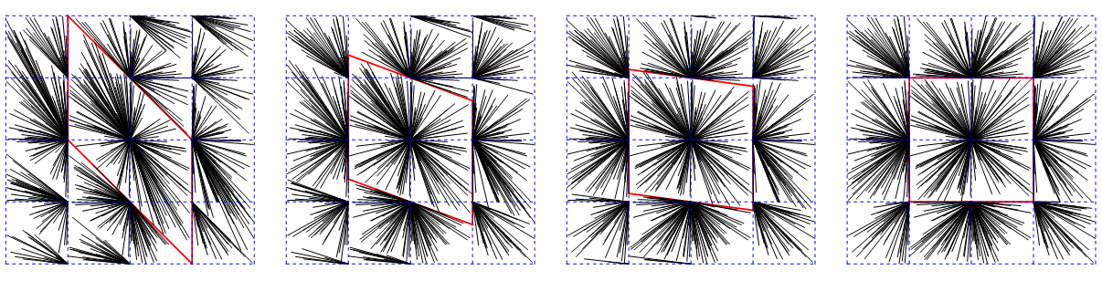
Figure 6: Quantization w.r.t $\|.\|_{A,\alpha}$, $\alpha\in\{0,1,2,\infty\}$ for spike trains $\eta=a_{1}\delta_{0}+a_{2}\delta_{1}$ with random $a_{i}\in[-2,2]$; the corresponding unit balls are marked red; the arrows are connecting points with their quantization points.

Like for threshold-based sampling Moser (2017); Moser and Lunglmayr (2019) we also obtain quasi isometry in the discrete case, though the situation and the way of proving it is different. Here in this context, we get it as a byproduct of Theorem 1.

Corollary 1 (LIF Quasi Isometry)

The norm $\|.\|_{A,\alpha}$, $\vartheta>0$, establishes quasi isometry for the LIF neuron model, i.e.,

$$\|\eta_{1}-\eta_{2}\|_{A,\alpha}-2\vartheta\leq\|\mbox{LIF}_{\vartheta,\alpha}(\eta_{1})-\mbox{LIF}_{\vartheta,\alpha}(\eta_{2})\|_{A,\alpha}\leq\|\eta_{1}-\eta_{2}\|_{A,\alpha}+2\vartheta$$ (16)

and asymptotic isometry, i.e.,

$$\lim_{\vartheta\rightarrow 0}\|\mbox{LIF}_{\vartheta,\alpha}(\eta_{1})-\mbox{LIF}_{\vartheta,\alpha}(\eta_{2})\|_{A,\alpha}=\|\eta_{1}-\eta_{2}\|_{A,\alpha}$$ (17)

for all $\eta_{1},\eta_{2}\in\mathbb{S}$.

Theorem 1 together with the quasi isometry property (16) immediately gives an answer to our Postulates 1 and 2 in Section 3 in terms of Corollary 2 and Corollary 3. Because of the discontinuity of thresholding the best what we can expect is an error bound in order of the threshold $\vartheta$. The error bound (2) in Corollary 2 caused by a small lag is remarkable as it asymptotically depends only on the threshold and the maximal spike amplitude and not, e.g., on the spike frequency. This property is typical for the Alexiewicz norm and related metrics such as the discrepancy measure and contrasts the Euclidean geometry and its related concept of measuring correlation, see also Moser et al. (2011). For the proof we refer to E.

Corollary 2 (Error Bound on Lag)

For $\eta=\sum_{i}a_{i}\delta_{t_{i}}\in\mathbb{S}$ and sufficiently small $\Delta t$ we get the error bound:

$$\left\|\mbox{LIF}_{\vartheta,\alpha}(\eta(\cdot-\Delta t))-\mbox{LIF}_{\vartheta,\alpha}(\eta(\cdot))\right\|_{A,\alpha} \leq$$

$$\max_{i}|a_{i}|+2\,\vartheta+\Delta t\,\alpha(\|\eta\|_{A,\alpha}+\max_{i}|a_{i}|)+O(\Delta t^{2}).$$

(1) together with the triangle inequality of the norm gives

$$\left\|\mbox{LIF}_{\vartheta+\varepsilon,\alpha}(\eta)-\eta+\eta-\mbox{LIF}_{\vartheta,\alpha}(\eta)\right\|_{A,\alpha} \leq$$

$$\left\|\mbox{LIF}_{\vartheta+\varepsilon,\alpha}(\eta)-\eta\right\|_{A,\alpha}+\left\|\mbox{LIF}_{\vartheta,\alpha}(\eta)-\eta\right\|_{A,\alpha} \leq 2\vartheta+\varepsilon,$$

proving Corollary 3.

Corollary 3 (Error Bound on Threshold Perturbation)

For $\varepsilon>0$ we have

$$\sup_{\eta\in\mathbb{S}}\left\|\mbox{LIF}_{\vartheta+\varepsilon,\alpha}(\eta)-\mbox{LIF}_{\vartheta,\alpha}(\eta)\right\|_{A,\alpha}\leq 2\vartheta+\varepsilon.$$ (18)

(1) can also be interpreted as spike train decomposition into a part that consists of spikes with amplitudes that are signed multiples of the threshold and a sub-threshold residuum. It is interesting that the first part can be further decomposed into a sum of unit Alexiewicz norm spike trains. See D for an example.

Theorem 2 (Spike Train Decomposition)

For any $\eta\in\mathbb{S}$ there is a $\psi\in\mathbb{S}$ with spike amplitudes that are integer multiples of the threshold and a below-threshold residuum spike train $\rho\in\mathbb{S}$ with $\|\rho\|_{A,\alpha}<\vartheta$, such that $\eta=\psi+\rho$, where $\psi=\mbox{LIF}_{\vartheta,\alpha}(\eta)$. Moreover, $\psi$ can be represented as sum of $\|.\|_{A,0}$-unit spike trains $\Delta\eta_{r}$, $r\in\{1,\ldots,a\}$, $a:=\|\psi\|_{A,0}$, i.e.,

$$\psi=\sum_{r=1}^{a}\Delta\eta_{r},$$ (19)

where $\|\Delta\eta_{r}\|_{A,0}=1$ for all $r$.

Proof.

Let $\eta_{0}:=\psi$ be the initial spike train with integer spike amplitudes $a_{i}^{(0)}\in\mathbb{Z}$. Assume that $\|\eta_{0}\|_{A,0}>1$. For convenience we define a sum over an empty index set to be zero, i.e., $\sum_{i\in\emptyset}a_{i}=0$. We will recursively define a sequence

$$\eta_{r}=\sum_{i=1}^{N^{(r)}}a_{i}^{(r)}\delta_{t_{i}},$$ (20)

of spike trains for $r=1,\ldots,N^{(0)}$ such that $\|\eta_{r}-\eta_{r-1}\|_{A,0}=1$ and $\eta_{N^{(0)}}=\emptyset$. Denote $N^{(r)}:=\|\eta_{r}\|_{A,0}$.

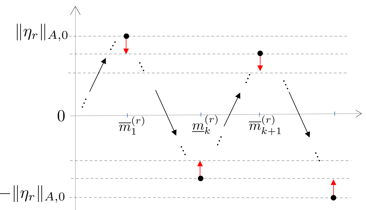
Figure 7: Peaks in spike decomposition algorithm. The subtraction of $\Delta\eta_{r}$ results in shifting the peaks towards the zero line, indicated by the red arrows.

If $N^{(r)}\geq 2$, then according to Fig. (7) we consider the peaks in the walk $S_{k}=\sum_{i=1}^{k}a_{i}^{(r)}$. Without loss of generality let us assume that the first peak is positive. For this we define recursively the corresponding top and bottom peak indexes $\overline{m}_{k}^{(r)}$, resp. $\underline{m}_{k}^{(r)}$ as follows.

$$\overline{m}_{1}^{(r)} := \min\{k>0:\sum_{i=1}^{k}a_{i}^{(r)}=N^{(r)}\},$$

$$\overline{m}_{k+1}^{(r)} := \min\{k>\overline{m}_{k}^{(r)}:\sum_{i=1}^{k}a_{i}^{(r)}\geq N^{(r)}-1\},$$ (21)

and, analogously,

$$\underline{m}_{k}^{(r)}:=\min\{m\in J=\{\overline{m}_{k}^{(r)}+1,\ldots,\overline{m}_{k+1}^{(r)}\}:\sum_{i=1}^{m}a_{i}^{(r)}=\min_{j\in J}\sum_{i=1}^{j}a_{i}^{(r)}\leq-1\}.$$ (22)

Based on (3.2) and (22) we define the spike train $\Delta\eta_{r+1}:=\sum_{i}d^{(r+1)}_{i}\delta_{t_{i}}$ as follows. Due to our assumption that the first peak is positive we define (otherwise $-1$)

$$d^{(r+1)}_{m_{1}}:=1.$$ (23)

For the subsequent peaks we consider the down and up intervals

$$\underline{J}_{k}:=\left\{\overline{m}_{k}^{(r)}+1,\ldots,\underline{m}_{k}^{(r)}\right\},\,\,\overline{J}_{k}:=\left\{\underline{m}_{k}^{(r)}+1,\ldots,\overline{m}_{k+1}^{(r)}\right\}.$$ (24)

We set $d^{(r+1)}_{i}:=0$ for all $t_{i}$ except the following cases. There are two cases for down intervals (analogously for up intervals):

• Case A. $\sum_{i\in\underline{J}_{k}}a_{i}^{(r)}\leq-2$ and there is an index $i\in\underline{J}_{k}:a_{i}^{(r)}\leq-2$, then we set

  $$d^{(r+1)}_{i}:=-2.$$ (25)

• Case B. $\sum_{i\in\underline{J}_{k}}a_{i}^{(r)}\leq-2$ and there is no index $i\in\underline{J}_{k}:a_{i}^{(r)}\leq-2$, then there are at least two indexes $i_{1},i_{2}$ such that $a_{i_{1}}^{(r)}+a_{i_{2}}^{(r)}\leq-2$. Thus, we set

  $$d^{(r+1)}_{i_{1}}:=-1,\\ d^{(r+1)}_{i_{2}}:=-1.$$

Analogously, we define the spikes for the up intervals, i.e., again distinguishing two cases.

• Case A. $\sum_{i\in\overline{J}_{k}}a_{i}^{(r)}\geq 2$ and there is an index $i\in\underline{J}_{k}:a_{i}^{(r)}\geq 2$, then we set

  $$d^{(r+1)}_{i}:=2.$$ (26)

• Case B. $\sum_{i\in\underline{J}_{k}}a_{i}^{(r)}\geq 2$ and there is no index $i\in\underline{J}_{k}:a_{i}^{(r)}\geq 2$, then there are at least two indexes $i_{1},i_{2}$ such that $a_{i_{1}}^{(r)}+a_{i_{2}}^{(r)}\geq 2$. Thus, we set

  $$d^{(r+1)}_{i_{1}}:=1,\\ d^{(r+1)}_{i_{2}}:=1.$$

Not that $\|\Delta\eta_{r+1}\|_{A,0}=1$ and $\|\eta_{r}-\Delta\eta_{r+1}\|_{A,0}=\|\eta_{r}\|_{A,0}-1$, since all peaks are shifted by $1$ towards the zero line. Since in each step the $\|.\|_{A,0}$ reduced by $1$, $\|\psi\|_{A,0}$ many steps are sufficient to represent $\psi=\sum_{r}\Delta\eta_{r}$. $\square$

4 Additive Spike Errors and a Resonance Phenomenon

Figure 8: Scheme for additive signal error propagation through a single LIF model.

In this section we first study the effect on the output of a single LIF neuron model when perturbing an input spike train $\eta$ by adding weighted spikes $\nu$, as illustrated in Fig. 8.

First of all we consider the special cases of zero and infinite leakage, i.e., $\alpha=0$, resp., $\alpha=\infty$, to obtain Lemma 2. For the proof see F.

Lemma 2 (Additive Error Bound for Integrate-and-Fire)

Let $\mbox{LIF}_{\vartheta,\alpha}$ be a LIF neuron model with $\alpha\in\{0,\infty\}$ and reset-to-mod re-initialization, then:

$$\forall\vartheta>0,\eta,\nu\in\mathbb{S}:\|\nu\|_{A,\alpha}\leq\vartheta\Rightarrow\|\mbox{LIF}_{\vartheta,\alpha}(\eta+\nu)-\mbox{LIF}_{\vartheta,\alpha}(\eta)\|_{A,\alpha}\leq\vartheta.$$ (27)

Based on Theorem 1 on characterizing LIF as signal-to-spike-train quantization and taking into account the special cases of $\alpha\in\{0,\infty\}$ of Lemma 2 we obtain a Lipschitz-style upper bound in terms of inequality (28) for a reset-to-mod LIF neuron, resp. in terms of (37) for SNNs based on reset-to-mod LIF neurons.

Theorem 3 (Liptschitz-Style Upper Bound for the LIF model)

For a reset-to-mod LIF neuron model with $\vartheta>0$ and $\alpha\in[0,\infty]$ and for all spike trains $\nu\in\mathbb{S}$ there holds the following inequality

$$\sup_{\eta\in\mathbb{S}}\left\|\mbox{LIF}_{\vartheta,\alpha}(\eta+\nu)-\mbox{LIF}_{\vartheta,\alpha}(\eta)\right\|_{A,\alpha}\leq\gamma(\alpha)\left\lceil\frac{1}{\vartheta}\|\nu\|_{A,\alpha}\right\rceil\vartheta,$$ (28)

where $\gamma(0)=\gamma(\infty)=1$ and $\gamma(\alpha)\in[2,3]$ for $\alpha\in(0,\infty)$.

Proof.

First of all note that

$$\xi(\vartheta,\alpha):=\sup_{\eta,\nu\in\mathbb{S}}\frac{\left\|\mbox{LIF}_{\vartheta,\alpha}(\eta+\nu)-\mbox{LIF}_{\vartheta,\alpha}(\eta)\right\|_{A,\alpha}}{\left\lceil\|\frac{1}{\vartheta}\nu\|_{A,\alpha}\right\rceil\vartheta}$$ (29)

is independent from $\vartheta$ although $\vartheta$ appears in (29), as shown in the following. Indeed, for given threshold $\vartheta>0$ let $\eta_{i}^{(\vartheta)}$ and $\nu_{i}^{(\vartheta)}$ be sequences for which the fraction in (29) converges to $\xi(\vartheta,\alpha)$, then $\widetilde{\eta_{i}}:=\eta_{i}^{(\vartheta)}/\vartheta$ and $\widetilde{\nu_{i}}:=\nu_{i}^{(\vartheta)}/\vartheta$ yield

$$\xi(\vartheta,\alpha)=\sup_{i}\frac{\vartheta\left\|\mbox{LIF}_{1,\alpha}(\widetilde{\eta_{i}}+\widetilde{\nu_{i}})-\mbox{LIF}_{1,\alpha}(\widetilde{\eta_{i}})\right\|_{A,\alpha}}{\left\lceil\|\frac{1}{\vartheta}\nu_{i}^{(\vartheta)}\|_{A,\alpha}\right\rceil\vartheta}=\xi(1,\alpha).$$ (30)

Now, define and use (13)

$$\gamma(\alpha) := \xi(1,\alpha)$$ (31)

$$= \sup_{\eta,\nu\in\mathbb{S}}\frac{\left\|\mbox{LIF}_{1,\alpha}(\eta+\nu)-(\eta+\nu)+\nu+\eta-\mbox{LIF}_{1,\alpha}(\eta)\right\|_{A,\alpha}}{\left\lceil\|\nu\|_{A,\alpha}\right\rceil}$$

$$\leq \sup_{\eta,\nu\in\mathbb{S}}\frac{2+\|\nu\|_{A,\alpha}}{\left\lceil\|\nu\|_{A,\alpha}\right\rceil}\leq 3<\infty.$$

Now, consider $\alpha\in(0,\infty)$ and the following example.

Example 1

Let $\eta=\sum_{k=1}^{3}a_{k}\delta_{t_{k}}$ for $t_{k}=k\varepsilon$, $\varepsilon>0$ and $(a_{1},a_{2},a_{3})=(-\frac{3}{2},1,\frac{3}{2})$, and $\nu=\sum_{k=1}^{3}b_{k}\delta_{t_{k}}$ with $(b_{1},b_{2},b_{3})=(1,-1,1)$ satisfying $\|\nu\|_{A,\alpha}=1$ for all $\alpha\in[0,\infty]$.

For $\alpha\in(0,\infty)$ we obtain for this example

$$\mbox{LIF}_{1,\alpha}(\eta) = -1\,\delta_{t_{1}}+0\,\delta_{t_{2}}+1\,\delta_{t_{3}},$$

$$\mbox{LIF}_{1,\alpha}(\eta+\nu) = 0\,\delta_{t_{1}}+0\,\delta_{t_{2}}+2\,\delta_{t_{3}}.$$ (32)

Therefore we get

$$\rho(\varepsilon,\alpha):=\|\mbox{LIF}_{1,\alpha}(\eta+\nu)-\mbox{LIF}_{1,\alpha}(\eta)\|_{A,\alpha} = \|1\,\delta_{t_{1}}+0\,\delta_{t_{2}}+1\,\delta_{t_{3}}\|_{A,\alpha}$$ (33)

$$= \left|1+e^{-2\varepsilon\alpha}\right|.$$

From $\lim_{\vartheta\rightarrow 0}\rho(\varepsilon,\alpha)=2$ for all $\alpha\in(0,\infty)$ we follow that $\gamma(\alpha)\geq 2$ for all $\alpha\in(0,\infty)$.

Now, let us check the special case $\alpha=0$. Without loss of generality we may assume that $\vartheta=1$. For this case we apply the spike train decomposition of Corollary 2, which allows us to represent $\nu=\sum_{k=1}^{a}\nu_{k}+\widetilde{\nu}$, where $a:=\left\lfloor\|\nu\|_{A,0}\right\rfloor$, $\|\nu_{k}\|_{A,0}=1$ and $\|\widetilde{\nu}\|_{A,0}<1$. Then, taking into account Lemma 2 and applying (13) on the telescope sum

$$\|\mbox{LIF}_{1,0}(\eta+\nu)-\mbox{LIF}_{1,0}(\eta)\|_{A,0}$$ (34)

$$= \|\,\mbox{LIF}_{1,0}(\eta+\nu_{1}+\ldots+\nu_{a}+\widetilde{\nu})-\mbox{LIF}_{1,0}(\eta+\nu_{2}+\ldots+\nu_{a}+\widetilde{\nu})$$

$$+\mbox{LIF}_{1,0}(\eta+\nu_{2}+\ldots+\nu_{a}+\widetilde{\nu})-\mbox{LIF}_{1,0}(\eta+\nu_{3}+\ldots+\nu_{a}+\widetilde{\nu})$$

$$\,\,\,\,\ldots$$

$$+\mbox{LIF}_{1,0}(\eta+\nu_{a}+\widetilde{\nu})-\mbox{LIF}_{1,0}(\eta+\widetilde{\nu})$$

$$+\mbox{LIF}_{1,0}(\eta+\widetilde{\nu})-\mbox{LIF}_{1,0}(\eta)\,\|_{A,0}$$

$$\leq \left\lceil\|\nu\|_{A,0}\right\rceil$$

we obtain $\gamma(0)\leq 1$. Since Example 1 gives

$$\mbox{LIF}_{1,0}(\eta) = -1\,\delta_{t_{1}}+0\,\delta_{t_{2}}+2\,\delta_{t_{3}},$$

$$\mbox{LIF}_{1,0}(\eta+\nu) = 0\,\delta_{t_{1}}+0\,\delta_{t_{2}}+2\,\delta_{t_{3}},$$ (35)

hence, $\|\mbox{LIF}_{1,0}(\eta+\nu)-\mbox{LIF}_{1,0}(\eta)\|_{A,0}=1$, we finally get $\gamma(0)=1$. The same way of reasoning on the telescope sum applies to the case $\alpha=\infty$, giving $\gamma(\infty)\leq 1$. Checking again Example 1, we get

$$\mbox{LIF}_{1,\infty}(\eta) = -1\,\delta_{t_{1}}+1\,\delta_{t_{2}}+1\,\delta_{t_{3}},$$

$$\mbox{LIF}_{1,\infty}(\eta+\nu) = 0\,\delta_{t_{1}}+0\,\delta_{t_{2}}+2\,\delta_{t_{3}},$$ (36)

hence, $\|\mbox{LIF}_{1,\infty}(\eta+\nu)-\mbox{LIF}_{1,\infty}(\eta)\|_{A,0}=\|1\,\delta_{t_{1}}-1\,\delta_{t_{2}}+1\,\delta_{t_{3}}\|_{A,0}=1$, showing that $\gamma(\infty)=1$. $\square$

Theorem 3 together with the triangle inequality of the norm $\|.\|_{A,\alpha}$ immediately yields a global upper bound on the norm difference of $\mbox{LIF}(\eta)$ and its perturbed version $\mbox{LIF}(\eta+\nu)$ for SNNs.

Theorem 4 (Global Lipschitz-Style Bound for SNNs)

Let the spiking neural network $\mbox{SNN}:\mathbb{S}^{N_{0}}\rightarrow\mathbb{S}^{(N_{L})}$ with reset-to-mod LIF neurons $\mbox{LIF}_{\vartheta,\alpha}$, $\vartheta=1$, be given by $[W^{(1)},\ldots,W^{(N_{L})}]$ according to (9), and let $(\nu_{1},\ldots,\nu_{N_{0}})$ be additive error spike trains in the corresponding input spike trains $(\eta_{1},\ldots,\eta_{N_{0}})$ , then for all output channels $\eta_{j}^{(N_{L})}$, $j\in\{1,\ldots,N_{L}\}$, we obtain the following error bound

$$\sup_{\eta_{i}}\left\|\mbox{SNN}\left((\eta_{i}+\nu_{i})_{i}\right)-\mbox{SNN}\left((\eta_{i})_{i}\right)\right\|_{A,\alpha}$$ (37)

$$\leq_{j} \Gamma_{\alpha}\circ\widetilde{W}^{(N_{L})}\left(\Gamma_{\alpha}\circ\widetilde{W}^{(N_{L}-1)}\cdots\left(\Gamma_{\alpha}\circ\widetilde{W}^{(1)}\left(\Gamma_{\alpha}\circ\nu_{A,\alpha}\right)\right)\right),$$

where $\|(c_{i,j})_{i,j}\|_{A,\alpha}:=((\|(c_{i,j})_{i,j}\|_{A,\alpha})_{i})$, $\leq_{j}$ refers to the $j$-th output channel on the left and the right hand side of the inequality, $\widetilde{W}^{(k+1)}:=\left(\left|w^{(k+1)}_{i_{k+1},i_{k}}\right|\right)_{i_{k+1},i_{k}}$, $\nu_{A,\alpha}:=\left(\left\|\nu_{1}\right\|_{A,\alpha},\ldots,\left\|\nu_{N_{0}}\right\|_{A,\alpha}\right),\Gamma_{\alpha}(x):=\left\lceil\gamma(\alpha)\,x\right\rceil$ and the rounding-up function $\left\lceil.\right\rceil$ is applied coordinate-wise.

5 Evaluation

In this section we look at numerical examples to demonstrate the main theoretical results of our paper, that is above all (13) on spike train quantization and its consequences in terms of quasi isometry, Corollary 1, the error bounds w.r.t time delay, Corollary 2 and the global Lipschitz-stlye upper bound for additive spike trains due to Theorem 3 for the LIF model, resp. Theorem 4 for LIF-based feedforward SNNs. See https://github.com/LunglmayrMoser/AlexSNN for Python and Mathematica code.

All the theoretical findings of this paper are based on the choice of reset-to-mod as re-initialization mode. Therefore, in the subsequent evaluations we also take the other reset modes into account to get an overview about the differences in the behavior. It is also instructive to look at the effect of alternative distance measures that are not equivalent to the Alexiewicz norm. We restrict this comparison to the Euclidean based norm (38). Other metrics for spike trains such as  Satuvuori and Kreuz (2018); Sihn and Kim (2019); Victor (2005) are not considered because they are motivated for other purposes than considered in our approach which aims at characterizing that topology of the vector space $\mathbb{S}$ which meets the Postulates 1 and 2 of Section 3. Therefore a detailed discussion on potential implications of the Alexiewicz topology (and its leaky variants) in the context of other proposed metrics is postponed for future study.

5.1 Spike Train Quantization due to (13)

Fig. 9 displays the quantization error in the Alexiewicz topology, i.e., $\|\mbox{LIF}_{\vartheta,\alpha}(\eta)-\eta\|_{A,\alpha}$-norm for the different reset variants: (a) reset-to-zero, (b) reset-by-subtraction, and, ours, (c) reset-to-mod. For large leaky parameter $\alpha$ all three variants tend to same error behavior. As expected according to Theorem 1 only in the reset-to-mod variant we can guarantee the bound of of Theorem 1. In contrast, Fig. 10 illustrates the effect of choosing the Euclidean topology as commonly used in the context of SNNs, i.e.,

$$\left\|\sum_{i=1}^{N}a_{i}\delta_{t_{i}}\right\|_{2,\alpha}:=\sqrt{\sum_{k=1}^{N}\left(\sum_{i=1}^{k}a_{i}e^{-\alpha(t_{k}-t_{i})}\right)^{2}}.$$ (38)

In contrast to the Alexiewicz topology and the reset-to-mod re-initialization of the LIF neuron there is no guarantee in the Euclidean metric to have a global upper bound for the quantization error, see Fig. (11).

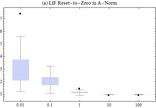
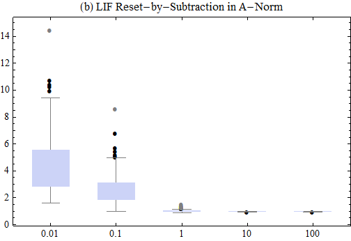
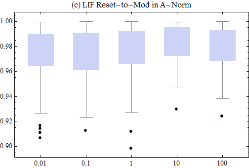
Figure 9: Distribution of the quantization error $\|\mbox{LIF}_{\vartheta,\alpha}(\eta)-\eta\|_{A,\alpha}$ for $\vartheta=1$, $\alpha\in\{0.01,0.1,1,10,100\}$ and the reset variants: (a) reset-to-zero, (b) reset-by-subtraction, and, (c) reset-to-mod (ours); the spike trains with $50$ spikes (at equidistant grid) are generated by uniformly distributed spike amplitudes in the range of $[-2,2]$; for each variant $100$ runs are performed.

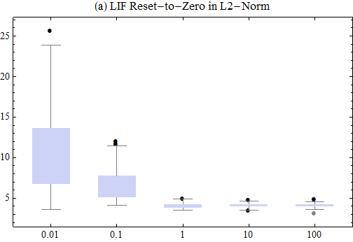
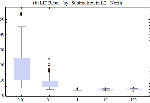
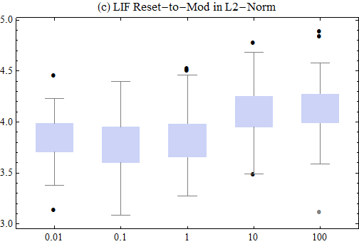
Figure 10: Like in Fig. 9 with $L_{2}$-based norm (38).

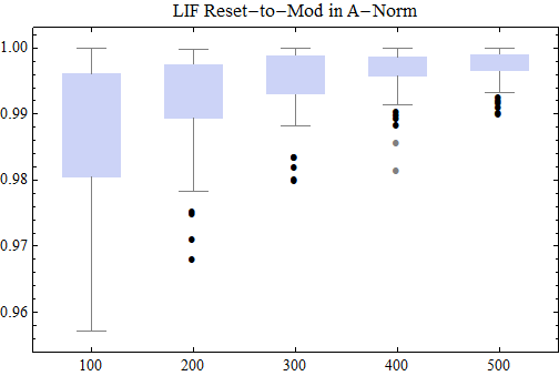
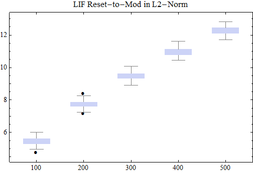
Figure 11: Like Fig. 9 and 10 for $\alpha=1$ but different numbers of spikes, $N\in\{100,\ldots,500\}$. While the quantization error in the Euclidean norm (38) increases with $N$ (right), due to Theorem 1 it remains strictly upper bounded by the threshold in the Alexiewicz topology (left). Note the concentration of measure effect in the Alexiewicz topology, see Vershynin .

5.2 Error Bounds regarding Postulates 1 and 2 and Quasi Isometry

Postulates 1 and 2 are covered by the inequalities (2), resp. (18), regarding time delay, resp. threshold deviation. Fig. 12 shows an example including the theoretical upper bound proven for the reset-to-mod variant together with the norm-errors resulting from our three re-initialization variants and different settings of the leakage parameter. For time delays the theoretical upper bound is guaranteed for sufficiently small time delays (see E). In this example the other re-initialization variants reset-by-subtraction and reset-to-zero show smaller errors compared to reset-to-mod . For threshold deviations it is the other way round and as guaranteed by (18) the reset-to-mod related dashed red line is strictly below the bound (black line) for all $\Delta\vartheta$.

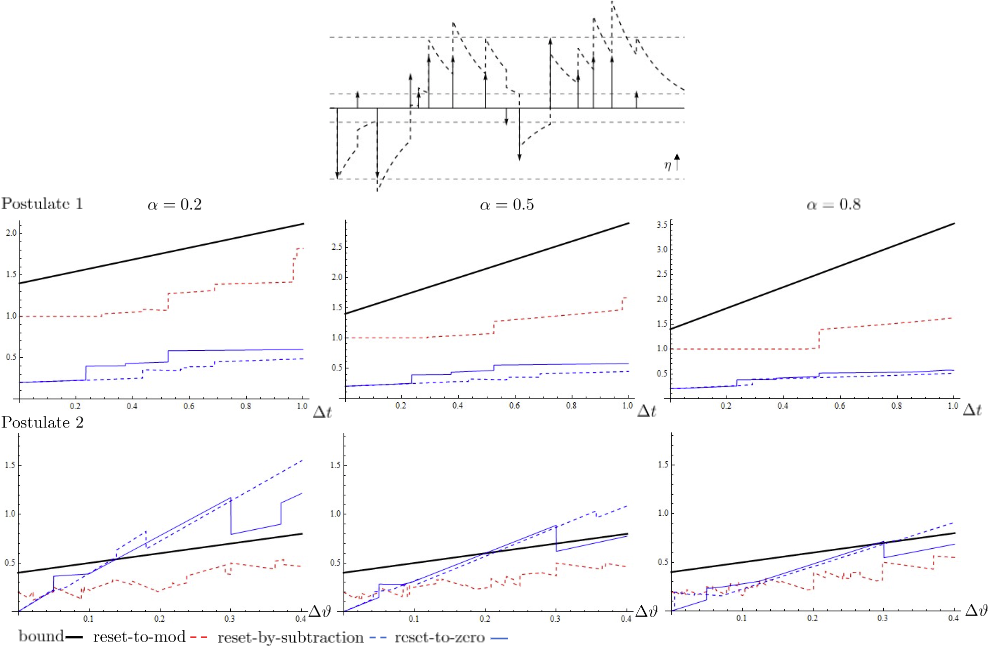
Figure 12: Evaluation of the effect of time delay $\Delta t$ (second row) and threshold deviations $\Delta\vartheta$ (third row) for a single LIF neuron for different $\alpha\in\{0.2,0.5,0.8\}$. The plots show the left side of the inequalities (2), resp. (18), for the three reset variants together with the bound (black line) given by the right side of the corresponding inequalities.

Like the data for spike train quantization, also the analysis of quasi isometry, see Fig.13, shows significant differences regarding the choice of the re-initialization mode.

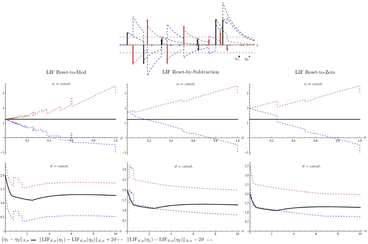
Figure 13: Evaluation of quasi isometry. Second and third row: Evaluation of $\|.\|_{A,\alpha}$-norm of $\eta_{1}-\eta_{2}$ after applying $\mbox{LIF}_{\vartheta,\alpha}$ for const. $\alpha=4$, second row, and const. $\vartheta=0.3$ for third row. Only reset-to-mod meets the conditions of quasi isometry due to (16).

5.3 Lipschitz-Style Upper Bound for LIF and SNNs

First we look at a single LIF neuron. Theorem 3 actually addresses two aspects. First, the global Lipschitz-style bound, and second, the observation that the upper bound constant $\gamma(\alpha)$ behaves different for $\alpha\in\{0,\infty\}$ and $\alpha\in(0,\infty)$. In Fig. 14 we compute this effect for different leakage parameters $\alpha$ and scaling factors $\lambda$ of the additive spike train $\nu$. As these $(\alpha,\lambda)$-plots show the amplification factor can be quite discontinuous and jagged. Different interfering $\nu$ signals can cause quite different shapes. The more it is remarkable that the amplification factor is globally bounded for all input spike trains irrespective of how many spikes they contain, and that for $\alpha=0$ (or, large) we have the tight bound of $\gamma(\alpha)=1$. For $\alpha\in(0,\infty)$ we find examples converging to $\gamma(\alpha)=2$ as proven in the Theorem. It is a conjecture that in fact $\gamma(\alpha)=2$, though in the proof we only have evidence that $\gamma(\alpha)\in[2,3]$. It remains an open question to analyze this resonance-type phenomenon in more detail. In contrast, the different shapes in the 3D plots comparing the re-initialization mode reset-to-mod (first row of 3D plots) with that of reset-to-zero can be explained more easily. Since a large $\alpha$ reduces the dependence on spikes in the past, hence approximating the behavior of reset-to-zero.

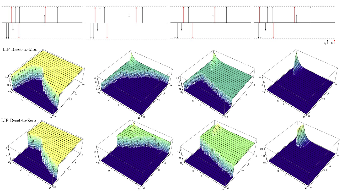
Figure 14: $(\alpha,\lambda)$-plot evaluations of the left hand side of inequality (28) for four variations of Example 1 for $\alpha\in[0,10]$ in the x-axis and scaling factor $\lambda\in[0,1]$ in the y-axis.

($\alpha$, $\lambda$)-plots of Fig. 14 look similar for SNNs. Due to Theorem 4 they are globally bounded for all input spike trains. However, the shape can be quite jagged and discontinuous as illustrated by Fig. 15 which shows an example for a $3$-layered SNN with

$$W^{(1)}=\left(\begin{array}[]{cc}1&1\\ 1&2\end{array}\right),\,W^{(2)}=\left(\begin{array}[]{cc}0.5&0\\ 0.5&0.5\\ 0&-0.5\end{array}\right),\,W^{(3)}=\left(\begin{array}[]{ccc}1&1&1\end{array}\right).$$ (39)

The comparison of the two examples in Fig. 15 show the sensitivity of time. After shifting the disturbing red spike to the green position the resulting $(\alpha,\lambda)$-plot breaks the symmetry causing a different characteristic of the shape. A detailed analysis of these effects is postponed to future research.

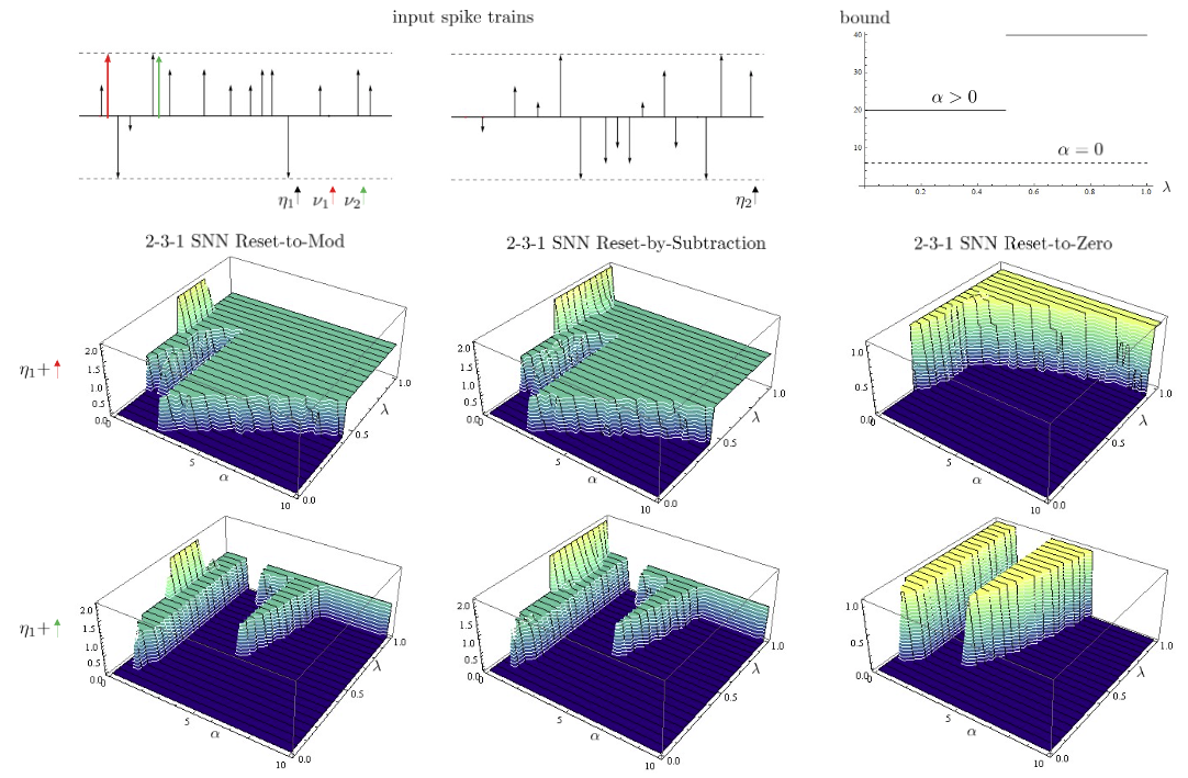
Figure 15: ($\alpha$, $\lambda$) evaluation of the left-hand side of the inequality (37) for the $2$-$3$-$1$ SNN given by the weight matrices (39) and the input spike trains $\eta_{i}$. The outer right graph depicts the right-hand side of the inequality (37) where the cases $\alpha=0$ and $\alpha>0$ are distinguished. The second row shows the ($\alpha$, $\lambda$) evaluation for the red additional spike, while the second row shows the evaluation with the green additional spike. In the the second row we disturb $\eta_{1}$ by the red spike, and accordingly, in the third row we add the green spike and the resulting 3D-plots of the measured error in the Alexiewicz norm like in Fig. 14 for the three different re-initialization modes as indicated.

6 Outlook and Conclusion

Our approach starts with the well-known observation that bio-inspired signal processing leads to a paradigm shift in contrast to the well-established technique of clock-based sampling and processing. Driven by the hypothesis that this paradigm shift must also manifest itself in its mathematical foundation, we started our analysis in terms of a top-down theory development by first searching for informative postulates. For the LIF neuron model (and SNNs based thereupon) our analysis shows that there is an underlying non-Euclidean geometry that governs its input-output behavior. As the central result of this paper, it turns out that this mapping can be fully characterized as signal-to-spike train quantization in the Alexiewicz norm, resp. its adaptation for a positive leakage parameter. While we gave a proof for this result for spike trains represented by a sequence of weighted Dirac impulses of arbitrary time intervals, we indicated in the Appendix that this quantization principle also holds for a wider class. Going beyond that, our conjecture is that the quantization error inequality will hold for all signals for which the formula is well-defined, but, that for being able to achieve this one will resort to an alternative concept of integration, namely the Henstock-Kurzweil integral which is related to the Alexiewicz topology. This remains to be worked out in follow-up research. So does the analysis of the resonance-like phenomenon of the in the context of the Lipschitz-style error bound. Another research direction is to explore the potential of our Alexiewicz norm-based approach for information coding and, more generally, for establishing a unified theory that incorporates low-level signal acquisition through event-based sampling and signal processing via feedback loops and learning strategies for high-level problem solving. Another thread running through the paper is the question of the choice and impact of the re-initialization variant. The quantization theorem is stated for the variant, which we coined reset-to-mod and results from applying reset-by-subtraction instantaneously in the case of spike amplitudes that exceed the threshold by a multiple. The resulting found properties such as quasi isometry or the error bound on time delay might be arguments for reset-to-mod, but in the end this study can only be seen as a starting point towards a more comprehensive theoretical foundation of bio-inspired signal processing taking its topological peculiarities into account.

Appendix A Proof of Theorem 1

We show the proof for $\alpha=0$. For $\alpha>0$ the argumentation is analogous.

From left to right. Consider a sequence $\eta_{n}$ of sub-threshold spike trains $\eta_{n}=\sum_{i_{n}}a_{i_{n}}^{(n)}\delta_{t_{i_{n}}}$, then an integrate-and-fire neuron never reaches the threshold $\theta>0$, i.e., for all $n$ and $m$ we have $|\sum_{i_{n}=0}^{m}a_{i_{n}}^{(n)}|<\theta$. Consequently, taking the limit w.r.t. $n$ we obtain the right-hand side of Equ. (1).

From right to left. Now, consider $\eta=\sum_{i}a_{i}\delta_{t_{i}}$ satisfying the inequality of the right-hand side of Equ. (1). If there is no spike in the output, the spike train is sub-threshold, i.e., $\eta\in C$, hence $\eta\in\overline{C}$. Assume that there is at least one spike in the output. Without loss of generality, let us assume that the first spike is positive. Then we define $i_{0}:=0$ and $i_{k}$ recursively by $i_{k+1}:=\min\{j:\sum_{i=i_{k}+1}^{j}=(-1)^{k}2\vartheta\}.$ Note that $a_{i}^{(\varepsilon)}:=a_{i}-(-1)^{k}\varepsilon a_{i}/\vartheta\}$ yields a spike train $\eta^{(\varepsilon)}\in C$ that converges to $\eta$.

Appendix B Unit Ball of $\|.\|_{A,0}$

In this section we characterize the unit ball $B_{A}$ of $\|.\|_{A}$ as sheared transform of the hypercube $[-1,1]^{N}$, i.e., $B_{A}=\{x\in\mathbb{R}^{N}:\,\|x\|_{A}\leq 1\}=\{x=Ty:\,y\in[-1,1]^{N}\}$, where

$$T=\left(\begin{array}[4]{ccccc}1&0&\cdots&\cdots&0\\ -1&1&0&\cdots&0\\ \vdots&\cdots&\ddots&\ddots&\vdots\\ 0&\cdots&\cdots&-1&1\end{array}\right).$$ (40)

Proof.

We are interested to characterize all $x=(x_{1},\ldots,x_{N})\in\mathbb{R}^{N}$ such that $\|x\|_{A}\leq 1$, i.e., $y_{n}:=\sum_{i=1}^{n}x_{i}\in[-1,1]$ for all $n\in\{1,\ldots,N\}$. Expressing $x_{i}$ in terms of $y_{i}$ means $y_{1}=x_{1}$, $y_{2}-y_{1}=x_{2}$, $\ldots$, $y_{N}-y_{N-1}=x_{N}$, that means $x=Ty$ due to (40). $\square$

Appendix C Proof for Spike Train Quantization for Dirac Impulses

We recall the proof from Moser and Lunglmayr (2023)

Theorem 5 (reset-to-mod LIF Neuron as $\|.\|_{A,\alpha}$-Quantization)

Given a LIF neuron model with reset-to-mod, the LIF parameters $\vartheta>0$ and $\alpha\in[0,\infty]$ and the spike train $\eta\in\mathbb{S}$ with amplitudes $a_{i}\in\mathbb{R}$. Then, $\mbox{LIF}_{\vartheta,\alpha}(\eta)$ is a $\vartheta$-quantization of $\eta$, i.e., the resulting spike amplitudes are multiples of $\vartheta$, where the quantization error is bounded by (13), hence $\mbox{LIF}_{\vartheta,\alpha}(\mbox{LIF}_{\vartheta,\alpha}(\eta)-\eta)=\emptyset$ and $\mbox{LIF}_{\vartheta,\alpha}\left(\mbox{LIF}_{\vartheta,\alpha}(\eta)\right)=\mbox{LIF}_{\vartheta,\alpha}(\eta)$.

Proof.

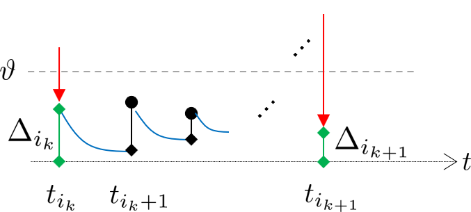
Figure 16: Illustration of Equation (42). The red arrows indicate reset-by-mod.

First of all, we introduce the following operation $\oplus$, which is associative and can be handled with like the usual addition if adjacent elements $a_{i}$ from a spike train $\eta=\sum_{i}a_{i}\delta_{t_{i}}$ are aggregated:

$$a_{i}\oplus a_{i+1}:=e^{-\alpha(t_{i+1}-t_{i})}a_{i}+a_{i+1}.$$ (41)

This way we get a simpler notation when aggregating convolutions, e.g.,

$$a_{i}\oplus\ldots\oplus a_{j}=\sum_{k=i}^{j}e^{-\alpha(t_{j}-t_{k})}a_{k}.$$

For the discrete version we re-define $a_{i_{k}}\oplus a_{i_{k+1}}:=\beta^{(i_{k+1}-i_{k})}a_{i_{k}}+a_{i_{k+1}}$, if $i_{k}$ and $i_{k+1}$ refer to adjacent spikes at time $i_{k}$, resp. $i_{k+1}$. Further, we denote $q[z]:=\mbox{sgn}(z)\,\left\lfloor|z|\right\rfloor$ which is the ordinary quantization due to integer truncation, e.g. $q[1.8]=1$, $q[-1.8]=-1$, where $\left\lfloor|z|\right\rfloor=\max\{n\in\mathbb{N}_{0}:\,n\leq|z|\}$.

After fixing notation let us consider a spike train $\eta=\sum_{j}a_{i}\delta_{t_{i}}$. Without loss of generality we may assume that $\vartheta=1$. We have to show that $\|\mbox{LIF}_{1,\alpha}(\eta)-\eta\|_{A,\alpha}<1$, which is equivalent to the discrete condition that $\forall n:\max_{n}\left|\sum_{i=1}^{n}\hat{a}_{i}\right|<1$, where $\eta-\mbox{LIF}_{1,\alpha}(\eta)=\sum_{i}\hat{a}_{i}\delta_{t_{i}}$. Set $\hat{s}_{k}:=\hat{a}_{0}\oplus\cdots\oplus\hat{a}_{k}$. We have to show that $\max_{k}|\hat{s}_{k}|<1$. The proof is based on induction and leads the problem back to the standard quantization by truncation.

Suppose that at time $t_{i_{k-1}}$ after re-initialization by reset-to-mod we get the residuum $\Delta_{i_{k-1}}$ as membrane potential that is the starting point for the integration after $t_{i_{k-1}}$. Note that

$$\mbox{LIF}_{1,\alpha}(\eta)|_{t=t_{k}}=q(\Delta_{i_{k-1}}\oplus a_{i_{k-1}+1}\cdots\oplus a_{i_{k}})$$

Then, as illustrated in Fig. 16 the residuum $\Delta_{i_{k}}$ at the next triggering event $t_{i_{k}}$ is obtained by the equation

$$\Delta_{i_{k}}=\Delta_{i_{k-1}}\oplus a_{i_{k-1}+1}\oplus\ldots\oplus a_{i_{k}}-q[\Delta_{i_{k-1}}\oplus\ldots\oplus a_{i_{k}}].$$ (42)

Note that due to the thresholding condition of LIF we have

$$|\Delta_{i_{k}}\oplus a_{i_{k}+1}\oplus\ldots\oplus a_{j}|<1$$ (43)

for $j\in\{i_{k}+1,\ldots,i_{k+1}-1\}$. For the $\oplus$-sums $\hat{s}_{i_{k}}$ we have

$$\hat{s}_{i_{k+1}}=\hat{s}_{i_{k}}\oplus a_{i_{k}+1}\cdots a_{i_{k+1}-1}\oplus\left(a_{i_{k+1}}-q[\Delta_{i_{k}}\oplus a_{i_{k}+1}\oplus\ldots\oplus a_{i_{k+1}}]\right).$$ (44)

Note that $\hat{s}_{0}=\Delta_{i_{0}}=a_{0}-q[a_{0}]$, then for induction we assume that up to index $k$ to have

$$\hat{s}_{i_{k}}=\Delta_{i_{k}}.$$ (45)

Now, using (45), Equation (44) gives

$$\hat{s}_{i_{k+1}} = \Delta_{i_{k}}\oplus a_{i_{k}+1}\oplus\ldots\oplus a_{i_{k+1}-1}\oplus\left(a_{i_{k+1}}-q[\Delta_{i_{k}}\oplus a_{i_{k+1}}\oplus\ldots\oplus a_{i_{k+1}}]\right)$$ (46)

$$= \Delta_{i_{k}}\oplus a_{i_{k}+1}\oplus\ldots\oplus a_{i_{k+1}-1}\oplus a_{i_{k+1}}-q[\Delta_{i_{k}}\oplus a_{i_{k+1}}\oplus\ldots\oplus a_{i_{k+1}}],$$

$$= \Delta_{i_{k+1}}$$

proving (45), which together with (43) ends the proof showing that $|\hat{s}_{k}|<1$ for all $k$.

$\square$

Appendix D Example for Spike Train Decomposition

Algorithm 2 summarizes this approach in the proof of Theorem 2 and Fig. 17 demonstrates an example.

Algorithm 2 Spike Train Decomposition

Step 0: Initialization: $\eta_{0}:=\eta$, $r=0$;
Step 1: Up and Down Intervals: Partition the time domain into up and down intervals $\overline{J}_{k}$, resp. $\underline{J}_{k}$ due to Equ. (24) based on the top and bottom peaks positions $\overline{m}_{k}$, resp., $\underline{m}_{k}$ in the resulting walk according to Equ. (3.2), resp. (22).
Step 2: Unit Discrepancy Delta: Define $\Delta\eta_{r+1}$ according to (23), (25), (• ‣ 3.2), (26) and (• ‣ 3.2).
Step 3: Subtraction: $\eta_{r+1}:=\eta_{r}-\Delta\eta_{r+1}$;
Step 4: Repeat steps 1, 2 and 3 until $r=\|\eta\|_{A,0}$ to obtain $\eta=\sum_{k=1}^{r}\Delta\eta_{k}$.

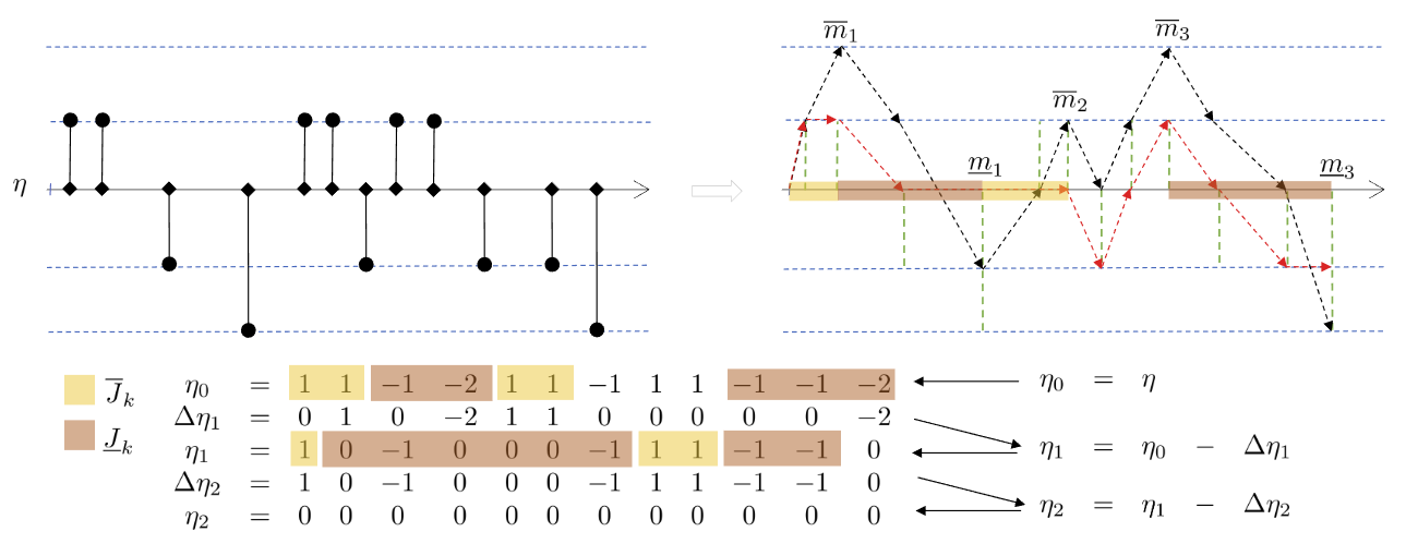
Figure 17: Example of decomposing a spike train $\eta$ with $\|\eta\|_{A,0}=2$ into a sum $\eta=\sum_{k=1,2}\Delta\eta_{k}$ with $\|\Delta\eta_{k}\|_{A,0}=1$, according to Algorithm 2. Top left: spike train $\eta$; Top right: illustration of first step with resulting walk and its top and bottom peaks due to (3.2) and (22). The red dashed line marks the resulting walk after subtracting $\Delta\eta_{1}$. Bottom: Recursive steps with highlighted up and down intervals according to (24).

Appendix E Error Bound on Lag, Corollary 2

The quasi-isometry property (16) yields

$$\left\|\mbox{LIF}_{\vartheta,\alpha}(\eta(\cdot-\Delta t))-\mbox{LIF}_{\vartheta,\alpha}(\eta)\right\|_{A,\alpha} \leq \left\|\eta(\cdot-\Delta t)-\eta\right\|_{A,\alpha}+2\vartheta.$$ (47)

Because of $e^{\alpha\Delta t}=1+\alpha\Delta t+O(\Delta t^{2})$ for $\Delta t\approx 0$, we get

$$\left\|\eta(\cdot-\Delta t)-\eta\right\|_{A,\alpha} = \max_{i}\left|\sum_{j=1}^{i-1}\left(a_{j}e^{-\alpha(t_{i}-t_{j})}-a_{j}e^{-\alpha(t_{i}-t_{j}-\Delta t)}\right)+a_{i}\right|$$ (48)

$$= \max_{n}\left|\sum_{j=1}^{n-1}a_{j}e^{-\alpha(t_{n}-t_{j})}\left(1-e^{\alpha\Delta t)}\right)+a_{n}\right|$$

$$= \max_{i}\left|(-\alpha\Delta t)\sum_{j=1}^{i-1}a_{j}e^{-\alpha(t_{i}-t_{j})}+a_{n}\right|+O(\|\eta\|_{A,\alpha}\Delta t)$$

$$\leq \alpha\,(\|\eta\|_{A,\alpha}+\max_{i}|a_{i}|)\,\Delta t+\max_{i}|a_{i}|,$$

which together with (47) proves (2).

Appendix F Proof of Lemma 2

First, let us check the case $\alpha=0$. Without loss of generality we may assume that $\vartheta=1$. Given spike trains $\eta,\nu\in\mathbb{S}$, $\eta=\sum_{i}a_{i}\delta_{t_{i}}$ and $\nu=\sum_{i}b_{i}\delta_{t_{i}}$ and suppose that $\|\nu\|_{A,0}\leq 1$. Denote by $p_{\eta}(t_{i}^{-})$ the membrane’s potential in the moment before triggering a spike w.r.t the input spike train $\eta$.

Indirectly, let us assume that there are three subsequent spikes with the same polarity (all negative or all positive) generated by adding $\nu$ to $\eta$. Without loss of generality we may assume that the polarity of these three spike events is negative. Let denote these time points by $t_{s_{1}}<t_{s_{2}}<t_{s_{3}}$ and let us consider the time point $t_{s_{0}}\leq t_{s_{1}}$ at which for the first time $\nu$ contributes to the negative spike event at $t_{s_{1}}$. Then, the first spiking event after $t_{s_{0}}$ is realized at $t_{s_{1}}$, which is characterized by

$$p_{\eta}(s_{1})-\sum_{i=s_{0}}^{s_{1}}b_{i}<[p_{\eta}(s_{1})]-1.$$ (49)

After the spike event at $t_{s_{1}}$ the re-initialization due to reset-to-mod takes place, meaning the reset of the membrane’s potential increase by $1$, resulting in the addition of $(1-\sum_{i=s_{0}}^{s_{1}}b_{i})$ to the original membrane’s potential $p_{\eta}(s_{1})$. Hence, we obtain for the second subsequent spike at $t_{s_{2}}$ the firing condition

$$p_{\eta}(s_{2})+(1-\sum_{i=s_{0}}^{s_{1}}b_{i})-\sum_{i>s_{1}}^{s_{2}}b_{i}<[p_{\eta}(s_{2})]-1,$$ (50)

thus,

$$p_{\eta}(s_{2})-[p_{\eta}(s_{2})]+2<\sum_{i=s_{0}}^{s_{2}}b_{i}.$$ (51)

Analogously, we obtain as characterizing condition for the third spiking event

$$p_{\eta}(s_{3})-[p_{\eta}(s_{3})]+3<\sum_{i=s_{0}}^{s_{3}}b_{i}.$$ (52)

Since $\|\nu\|_{A,0}\leq 1$, i.e., $|\sum_{i=1}^{k}b_{i}|\leq 1$ for all $k$ it follows that $|\sum_{i=k_{1}}^{k_{2}}b_{i}|=|\sum_{i=1}^{k_{2}}b_{i}-\sum_{i=1}^{k_{1}-1}b_{i}|\leq 2$. Which applied to (52) yields the contradiction

$$p_{\eta}(s_{3})-[p_{\eta}(s_{3})]+3<\sum_{i=s_{0}}^{s_{3}}b_{i}\leq 2,$$ (53)

namely, $-1<p_{\eta}(s_{3})-[p_{\eta}(s_{3})]\leq-1$. Therefore, there are at most $2$ subsequently triggered additional spikes by adding $\nu$.

The same way of reasoning, now with Equ. (50), shows that the first occurrence of an added spike can only be a single event which if any has to be followed by a spike event with different polarity. All together this means that $\|\mbox{LIF}_{1,0}(\eta+\nu)\|_{A,0}-\mbox{LIF}_{1,0}(\eta)\|_{A,0}\leq 1$.
The second case of $\alpha=\infty$, i.e., $\|\nu\|_{A,\infty}=\max_{i}|b_{i}|\leq 1$ reduces to the standard quantization of integer truncation, i.e., to show that $\max_{i}|[a_{i}+b_{i}]-[a_{i}]|\leq 1$, which follows from the fact that $-1\leq a_{i}-[a_{i}]+b_{i}<2$ for positive $a_{i}$ and $-2<a_{i}-[a_{i}]+b_{i}\leq 1$ for negative $a_{i}$.

References

- Gerstner et al. [2014] Wulfram Gerstner, Werner M. Kistler, Richard Naud, and Liam Paninski. Neuronal Dynamics: From Single Neurons to Networks and Models of Cognition. Cambridge University Press, USA, 2014. ISBN 1107635195.
- Tavanaei et al. [2019] Amirhossein Tavanaei, Masoud Ghodrati, Saeed Reza Kheradpisheh, Timothée Masquelier, and Anthony Maida. Deep learning in spiking neural networks. Neural Networks, 111:47–63, 2019. ISSN 0893-6080. doi:https://doi.org/10.1016/j.neunet.2018.12.002. URL https://www.sciencedirect.com/science/article/pii/S0893608018303332.
- Nunes et al. [2022] João D. Nunes, Marcelo Carvalho, Diogo Carneiro, and Jaime S. Cardoso. Spiking neural networks: A survey. IEEE Access, 10:60738–60764, 2022. doi:10.1109/ACCESS.2022.3179968.
- Guo et al. [2021] Wenzhe Guo, Mohammed E. Fouda, Ahmed M. Eltawil, and Khaled Nabil Salama. Neural coding in spiking neural networks: A comparative study for robust neuromorphic systems. Frontiers in Neuroscience, 15, 2021. ISSN 1662-453X. doi:10.3389/fnins.2021.638474. URL https://www.frontiersin.org/articles/10.3389/fnins.2021.638474.
- Miskowicz [2006] Marek Miskowicz. Send-on-delta concept: An event-based data reporting strategy. Sensors, 6(1):49–63, 2006. ISSN 1424-8220. doi:10.3390/s6010049. URL http://www.mdpi.com/1424-8220/6/1/49/.
- Liu et al. [2014] Shih-Chii Liu, Tobi Delbruck, Adrian Indiveri, Giacomo abd Whatley, and Rodney Douglas. Event-Based Neuromorphic Systems. John Wiley & Sons, Ltd, 2014. ISBN 9780470018491. doi:10.1002/9781118927601.
- Yousefzadeh and Sifalakis [2022] Amirreza Yousefzadeh and Manolis Sifalakis. Delta activation layer exploits temporal sparsity for efficient embedded video processing. In 2022 International Joint Conference on Neural Networks (IJCNN), pages 01–10, 2022. doi:10.1109/IJCNN55064.2022.9892578.
- Amir et al. [2017] Arnon Amir, Brian Taba, David Berg, Timothy Melano, Jeffrey McKinstry, Carmelo Di Nolfo, Tapan Nayak, Alexander Andreopoulos, Guillaume Garreau, Marcela Mendoza, Jeff Kusnitz, Michael Debole, Steve Esser, Tobi Delbruck, Myron Flickner, and Dharmendra Modha. A low power, fully event-based gesture recognition system. In 2017 IEEE Conference on Computer Vision and Pattern Recognition (CVPR), pages 7388–7397, 2017. doi:10.1109/CVPR.2017.781.
- Wu et al. [2018] Jibin Wu, Yansong Chua, Malu Zhang, Haizhou Li, and Kay Chen Tan. A spiking neural network framework for robust sound classification. Frontiers in Neuroscience, 12, 2018. ISSN 1662-453X. doi:10.3389/fnins.2018.00836. URL https://www.frontiersin.org/articles/10.3389/fnins.2018.00836.
- Wu et al. [2020] Jibin Wu, Emre Y?lmaz, Malu Zhang, Haizhou Li, and Kay Chen Tan. Deep spiking neural networks for large vocabulary automatic speech recognition. Frontiers in Neuroscience, 14, 2020. ISSN 1662-453X. doi:10.3389/fnins.2020.00199. URL https://www.frontiersin.org/articles/10.3389/fnins.2020.00199.
- Hassan et al. [2018] Amr M. Hassan, Aya F. Khalaf, Khaled S. Sayed, Hai Helen Li, and Yiran Chen. Real-time cardiac arrhythmia classification using memristor neuromorphic computing system. 2018 40th Annual International Conference of the IEEE Engineering in Medicine and Biology Society (EMBC), pages 2567–2570, 2018.
- Kabilan and Muthukumaran [2021] R. Kabilan and N. Muthukumaran. A neuromorphic model for image recognition using snn. In 2021 6th International Conference on Inventive Computation Technologies (ICICT), pages 720–725, 2021. doi:10.1109/ICICT50816.2021.9358663.
- Yamazaki et al. [2022] Kashu Yamazaki, Viet-Khoa Vo-Ho, Darshan Bulsara, and Ngan Le. Spiking neural networks and their applications: A review. Brain Sciences, 12(7):863, Jun 2022. doi:10.3390/brainsci12070863. URL https://dx.doi.org/10.3390/brainsci12070863.
- Yang et al. [2022] Helin Yang, Kwok-Yan Lam, Liang Xiao, Zehui Xiong, Hao Hu, Dusit Niyato, and H. Vincent Poor. Lead federated neuromorphic learning for wireless edge artificial intelligence. Nature Communications, 13(1):1–12, December 2022. doi:10.1038/s41467-022-32020-. URL https://ideas.repec.org/a/nat/natcom/v13y2022i1d10.1038_s41467-022-32020-w.html.
- Dethier et al. [2013] Julie Dethier, Paul Nuyujukian, Stephen I Ryu, Krishna V Shenoy, and Kwabena Boahen. Design and validation of a real-time spiking-neural-network decoder for brain-machine interfaces. Journal of Neural Engineering, 10(3):036008, apr 2013. doi:10.1088/1741-2560/10/3/036008. URL https://dx.doi.org/10.1088/1741-2560/10/3/036008.
- Gege et al. [2021] Zhan Gege, Zuoting Song, Tao Fang, Yuan Zhang, Song Le, Xueze Zhang, Shouyan Wang, Yifang Lin, Jie Jia, Lihua Zhang, and Xiaoyang Kang. Applications of spiking neural network in brain computer interface. pages 1–6, 02 2021. doi:10.1109/BCI51272.2021.9385361.
- Deng et al. [2020] Lei Deng, Yujie Wu, Xing Hu, Ling Liang, Yufei Ding, Guoqi Li, Guangshe Zhao, Peng Li, and Yuan Xie. Rethinking the performance comparison between snns and anns. Neural Networks, 121:294–307, 2020. ISSN 0893-6080. doi:https://doi.org/10.1016/j.neunet.2019.09.005. URL https://www.sciencedirect.com/science/article/pii/S0893608019302667.
- Bouvier et al. [2019] Maxence Bouvier, Alexandre Valentian, Thomas Mesquida, Francois Rummens, Marina Reyboz, Elisa Vianello, and Edith Beigné. Spiking neural networks hardware implementations and challenges. ACM Journal on Emerging Technologies in Computing Systems (JETC), 15:1 – 35, 2019.
- DeBole et al. [2019] Michael V. DeBole, Brian Taba, Arnon Amir, Filipp Akopyan, Alexander Andreopoulos, William P. Risk, Jeff Kusnitz, Carlos Ortega Otero, Tapan K. Nayak, Rathinakumar Appuswamy, Peter J. Carlson, Andrew S. Cassidy, Pallab Datta, Steven K. Esser, Guillaume Garreau, Kevin L. Holland, Scott Lekuch, Michael Mastro, Jeffrey L. McKinstry, Carmelo di Nolfo, Brent Paulovicks, Jun Sawada, Kai Schleupen, Benjamin Shaw, Jennifer L. Klamo, Myron D. Flickner, John V. Arthur, and Dharmendra S. Modha. Truenorth: Accelerating from zero to 64 million neurons in 10 years. Computer, 52(5):20–29, 2019. doi:10.1109/MC.2019.2903009. URL https://doi.org/10.1109/MC.2019.2903009.
- Ostrau et al. [2022] Christoph Ostrau, Christian Klarhorst, Michael Thies, and Ulrich Rückert. Benchmarking neuromorphic hardware and its energy expenditure. Frontiers in Neuroscience, 16, 2022. ISSN 1662-453X. doi:10.3389/fnins.2022.873935. URL https://www.frontiersin.org/articles/10.3389/fnins.2022.873935.
- Michaelis et al. [2022] Carlo Michaelis, Andrew B. Lehr, Winfried Oed, and Christian Tetzlaff. Brian2loihi: An emulator for the neuromorphic chip loihi using the spiking neural network simulator brian. Frontiers in Neuroinformatics, 16, 2022. ISSN 1662-5196. doi:10.3389/fninf.2022.1015624. URL https://www.frontiersin.org/articles/10.3389/fninf.2022.1015624.
- Moser and Natschläger [2014] Bernhard A. Moser and Thomas Natschläger. On stability of distance measures for event sequences induced by level-crossing sampling. IEEE Transactions on Signal Processing, 62(8):1987–1999, 2014. doi:10.1109/TSP.2014.2305642.
- Moser [2015] Bernhard Alois Moser. Stability of threshold-based sampling as metric problem. In International Conference on Event-based Control, Communication, and Signal Processing, EBCCSP 2015, Krakow, Poland, June 17-19, 2015, pages 1–8. IEEE, 2015. doi:10.1109/EBCCSP.2015.7300692. URL https://doi.org/10.1109/EBCCSP.2015.7300692.
- Moser [2016] Bernhard Alois Moser. On preserving metric properties of integrate-and-fire sampling. In Second International Conference on Event-based Control, Communication, and Signal Processing, EBCCSP 2016, Krakow, Poland, June 13-15, 2016, pages 1–7. IEEE, 2016. doi:10.1109/EBCCSP.2016.7605276. URL https://doi.org/10.1109/EBCCSP.2016.7605276.
- Moser [2017] Bernhard A. Moser. Similarity recovery from threshold-based sampling under general conditions. IEEE Transactions on Signal Processing, 65(17):4645–4654, 2017. doi:10.1109/TSP.2017.2712121.
- Moser and Lunglmayr [2019] Bernhard A. Moser and Michael Lunglmayr. On quasi-isometry of threshold-based sampling. IEEE Transactions on Signal Processing, 67(14):3832–3841, 2019. doi:10.1109/TSP.2019.2919415.
- Lapicque [1907] Louis Lapicque. Recherches quantitatives sur l’excitation électrique des nerfs traitée comme une polarisation. J. Physiol. Pathol. Gen., 9:620–635, 1907.
- Dayan and Abbott [2001] Peter Dayan and L. F. Abbott. Theoretical Neuroscience: Computational and Mathematical Modeling of Neural Systems. The MIT Press, 2001.
- Eshraghian et al. [2021] Jason K. Eshraghian, Max Ward, Emre Neftci, Xinxin Wang, Gregor Lenz, Girish Dwivedi, Mohammed Bennamoun, Doo Seok Jeong, and Wei D. Lu. Training spiking neural networks using lessons from deep learning, 2021. URL https://arxiv.org/abs/2109.12894.
- Bohte et al. [2000] Sander M. Bohte, Joost N. Kok, and Johannes A. La Poutré. Spikeprop: backpropagation for networks of spiking neurons. In ESANN, pages 419–424, 2000.
- Finch [2018] Steven R. Finch. How far might we walk at random?, 2018. URL https://arxiv.org/abs/1802.04615.
- Jain and Orey [1968] N. Jain and S. Orey. On the range of random walk. Israel J. Math., 6:373–380, 1968.
- Moser [2012] Bernhard A. Moser. Geometric characterization of Weyl’s discrepancy norm in terms of its n-dimensional unit balls. Discret. Comput. Geom., 48(4):793–806, 2012. doi:10.1007/s00454-012-9454-0. URL https://doi.org/10.1007/s00454-012-9454-0.
- Chazelle [2000] B. Chazelle. The Discrepancy Method: Randomness and Complexity. Cambridge University Press, 2000.
- Moser [2011] Bernhard A. Moser. A similarity measure for image and volumetric data based on hermann weyl’s discrepancy. IEEE Trans. Pattern Anal. Mach. Intell., 33(11):2321–2329, 2011. doi:10.1109/TPAMI.2009.50. URL https://doi.org/10.1109/TPAMI.2009.50.
- Weyl [1916] Hermnann Weyl. Über die Gleichverteilung von Zahlen mod. Eins. Math. Ann., 77:313–352, 1916.
- Alexiewicz [1948] Andrzej Alexiewicz. Linear functionals on denjoy-integrable functions. Colloq. Math., 1:289–293, 1948.