HyperE2VID: Improving Event-Based Video Reconstruction via Hypernetworks

Abstract

Event-based cameras are becoming increasingly popular for their ability to capture high-speed motion with low latency and high dynamic range. However, generating videos from events remains challenging due to the highly sparse and varying nature of event data. To address this, in this study, we propose HyperE2VID, a dynamic neural network architecture for event-based video reconstruction. Our approach uses hypernetworks and dynamic convolutions to generate per-pixel adaptive filters guided by a context fusion module that combines information from event voxel grids and previously reconstructed intensity images. We also employ a curriculum learning strategy to train the network more robustly. Experimental results demonstrate that HyperE2VID achieves better reconstruction quality with fewer parameters and faster inference time than the state-of-the-art methods.

I Introduction

In the past decade, the field of computer vision has seen astonishing progress in many different tasks, thanks to modern deep learning methodologies and recent neural architectures. But, despite all these advances, current artificial vision systems still fall short on dealing with some real-world situations involving high-speed motion scenes with high dynamic range, as compared to their biological counterparts. Some of these shortcomings can be attributed to the classical frame-based acquisition and processing pipelines, since the traditional frame-based sensors have some problems such as motion blur and low dynamic range due to the underlying basic principles used for collecting light.

The recently developed event cameras have the potential to eliminate the aforementioned issues by incorporating novel bio-inspired vision sensors which contain pixels that are asynchronous and work independently from each other [1]. Each pixel is sensitive to local relative light intensity variations, and when this variation exceeds a threshold, they generate signals called events, in continuous time. Therefore, the data output from these cameras is a stream of asynchronous events, where each event encodes the pixel location ($x,y$) and polarity $p\in\{+1,-1\}$ of the intensity change, together with a precise timestamp $t$. The event stream has a highly varying rate depending on the scene details such as brightness change, motion, and texture. These working principles of event cameras bring many advantages compared to traditional frame-based cameras, such as high dynamic range, high temporal resolution, and low latency. Due to the numerous advantages it offers, event data has been increasingly incorporated into various recognition tasks, including object detection [2], semantic segmentation [3], and fall detection [4]. Furthermore, event data has been utilized in challenging robotic applications that require high-speed perception, such as an object-catching quadrupedal robot [5] and an ornithopter robot capable of avoiding dynamic obstacles [6].

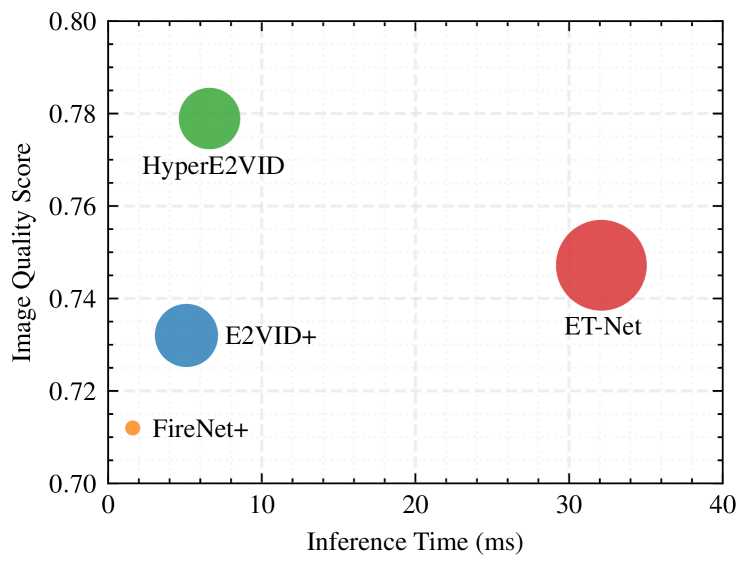
Figure 1: Comparison of our HyperE2VID method with state-of-the-art event-based video reconstruction methods based on image quality and inference time. Image quality scores are calculated by normalizing and averaging each of the quantitative scores reported in Table I, where normalization maps the best and worst possible score for each metric to $1.0$ and $0.0$. Inference times are measured as described in Section IV-G. Circle sizes indicate the number of model parameters, as detailed in Table III. For the clarity of presentation, the methods with lower image quality scores are not included.

Despite its desirable properties, humans can not directly interpret event streams as we do for intensity images, and high-quality intensity images are the most natural way to understand visual data. Hence, the task of reconstructing intensity images from events has long been a cornerstone in event-based vision literature. Another benefit of reconstructing high-quality intensity images is that one can immediately apply successful frame-based computer vision methods to the reconstruction results to solve various tasks.

Recently, deep learning based methods have obtained impressive results in the task of video reconstruction from events (e.g. [7, 8, 9]). To use successful deep architectures in conjunction with event-based data, these methods typically group events in time windows and accumulate them into grid-structured representations like 3D voxel grids through which the continuous stream of events is transformed into a series of voxel grid representations. These grid-based representations can then be processed with recurrent neural networks (RNNs), where each of these voxel grids is consumed at each time step.

Since events are generated asynchronously only when the intensity of a pixel changes, the resulting event voxel grid is a sparse tensor, incorporating information only from the changing parts of the scene. The sparsity of these voxel grids is also highly varying. This makes it hard for neural networks to adapt to new data and leads to unsatisfactory video reconstructions that contain blur, low contrast, or smearing artifacts ([7, 8, 10]). Recently, Weng et al. [9] proposed to incorporate a Transformer [11] based module to an event-based video reconstruction network in order to better exploit the global context of event tensors. This complex architecture improves the quality of reconstructions, but at the expense of higher inference times and larger memory consumption.

The methods mentioned above try to process the highly varying event data with static networks, in which the network parameters are kept fixed after training. Concurrently, there has been a line of research that investigates dynamic network architectures that allow the network to adapt its parameters dynamically according to the input supplied at inference time. A well-known example of this approach is the notion of hypernetworks [12], which are smaller networks that are used to dynamically generate weights of a larger network at inference time, conditioned on the input. This dynamic structure allows the neural networks to increase their representation power with only a minor increase in computational cost [13].

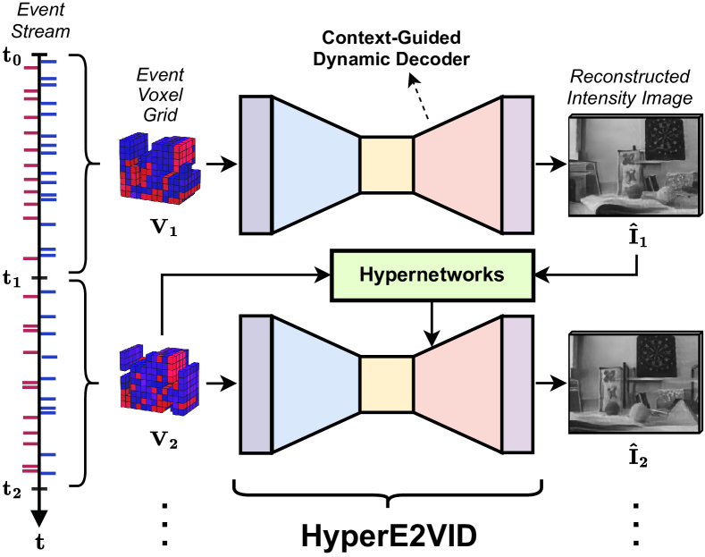
Figure 2: HyperE2VID uses a recurrent encoder-decoder backbone, consuming an event voxel grid at each timestep. It enhances this architecture by employing per-pixel, spatially-varying dynamic convolutions at the decoder, whose parameters are generated dynamically at inference time via hypernetworks.

In this work, we present HyperE2VID which improves the current state-of-the-art in terms of image quality and efficiency (see Fig. 1) by employing a dynamic neural network architecture via hypernetworks. Our proposed model utilizes a main network with a convolutional recurrent encoder-decoder architecture, similar to E2VID [7]. We enhance this network by employing dynamic convolutions, whose parameters are generated dynamically at inference time. These dynamically generated parameters are also spatially varying such that there exists a separate convolutional kernel for each pixel, allowing them to adapt to different spatial locations as well as each input. This spatial adaptation enables the network to learn and use different filters for static and dynamic parts of the scene where events are generated at low and high rates, respectively. We design our hypernetwork architecture in order to avoid the high computational cost of generating per-pixel adaptive filters via filter decomposition as in [14].

Fig. 2 presents an overview of our proposed method, HyperE2VID, for reconstructing video from events. Our approach is designed to guide the dynamic filter generation through a context that represents the current scene being observed. To achieve this, we leverage two complementary sources of information: events and images. We incorporate a context fusion module in our hypernetwork architecture to combine information from event voxel grids and previously reconstructed intensity images. These two modalities complement each other since intensity images capture static parts of the scene better, while events excel at dynamic parts. By fusing them, we obtain a context tensor that better represents both static and dynamic parts of the scene. This tensor is then used to guide the dynamic per-pixel filter generation. We also employ a curriculum learning strategy to train the network more robustly, particularly in the early epochs of training when the reconstructed intensity images are far from optimal.

To the best of our knowledge, this is the first work that explores the use of hypernetworks and dynamic convolutions for event-based video reconstruction. The closest to our work is SPADE-E2VID [10] where the authors employ adaptive feature denormalization in decoder blocks of the E2VID architecture. Rather than feature denormalization, we directly generate per-pixel dynamic filters via hypernetworks for the first decoder block. Specifically, our contributions can be summarized as follows:

• We propose the first dynamic network architecture for the task of video reconstruction from events, where we extend existing static architectures with hypernetworks, dynamic convolutional layers, and a context fusion block.

• We show via experiments that this dynamic architecture can generate higher-quality videos than previous state-of-the-art, while also reducing memory consumption and inference time.

II Related Work

II-A Event-Based Video Reconstruction

Reconstructing intensity images from events is a popular topic in event-based vision literature, involving approaches with different assumptions and processing methodologies. Earlier works generally rely on some limiting assumptions such as known or restricted camera movement, static scenes, or brightness constancy. On the other hand, recent deep learning based methods incorporate natural image priors in their models through the learning process.

In one of the earliest works, Cook et al. [15] proposed a bipartite-graph-like network to simultaneously estimate multiple quantities of interest such as intensity image, spatial gradients, and optical flow. Kim et al. [16] presented a filter-based method to simultaneously estimate scene gradients and ego-motion assuming that the camera only makes rotating motion. They proposed to employ Poisson integration [17] to reconstruct intensity images from the spatial gradient map. In their follow-up work [18], the authors extended this method to handle free 6-DOF camera motion. Barua et al. [19] learned a patch-based sparse dictionary from simulation data using K-SVD algorithm [20] and used this dictionary to obtain gradient images from events, followed by Poisson integration [17] to reconstruct intensity images. Bardow et al. [21] solved a variational optimization problem to simultaneously estimate intensity image and optical flow field, under the assumption of brightness constancy. Munda et al. [22] also proposed an optimization-based method where they considered a spatio-temporal volume of events and a lower dimensional manifold in this volume, defined by the timestamp of the latest event for each pixel. They minimized an energy function consisting of a data fidelity term based on direct integration of events and a manifold regularisation term. Scheerlinck et al. [23] employed a per-pixel temporal high-pass filter before integration to reduce accumulated noise and enable continuous-time intensity reconstruction through event-by-event processing, as a form of direct integration.

The last few years have witnessed many works that utilize neural networks and deep learning methodologies for the task of intensity image reconstruction. Wang et al. [24] represented groups of events with spatio-temporal voxel grids and fed them to a conditional GAN to output intensity images. Rebecq et al. [7] proposed a recurrent fully convolutional network called E2VID to which they input voxel grids of events to produce an intensity image. They trained this network on a large synthetic dataset generated with ESIM [25] using the perceptual loss of [26] and showed that this generalizes well to real event data at test time. As a follow-up study [27], the authors employed temporal consistency loss [28] to minimize temporal artifacts. Scheerlinck et al. [29] replaced E2VID with a lightweight recurrent network called FireNet, and showed that this can achieve comparable performance while having much less memory consumption and faster inference. Stoffregen et al. [8] further improved the results of E2VID and FireNet by matching statistics of synthetic training data to that of real-world test data. Zhang et al. [30] argued that the reconstruction performance of E2VID deteriorates when operated with low-light event data, and proposed a novel unsupervised domain adaptation network to generate intensity images as if captured in daylight, from event data of low-light scenes. Cadena et al. [10] employed spatially-adaptive denormalization (SPADE) [31] layers in E2VID architecture and argue that this improves the quality of early frames in the reconstructed videos. Weng et al. [9] incorporated a Transformer [11] based module to the CNN-based encoder-decoder architecture of E2VID, to better exploit the global context of event tensors. Mostafavi et al. [32] presented a network to generate super-resolved intensity images from events, and train this with a synthetic dataset. Similarly, Wang et al. [33] introduced a network that can also perform image restoration and super-resolution, which is trained in an unsupervised manner by employing an adversarial loss. Paredes-Vallés and de Croon [34] presented a self-supervised learning approach based on event-based photometric constancy assumption [35] to simultaneously estimate optical flow and intensity images. Zou et al. [36] collected high-speed and high dynamic range ground truth images corresponding to event streams with a novel imaging system, and use this real-world data together with a synthetic dataset to train their neural network. Zhu et al. [37] used a deep spiking neural network (SNN) architecture that can achieve comparable performance in a more computationally efficient way. Zhang et al. [38] formulated the event-based image reconstruction task as a linear inverse problem based on optical flow and showed that one can use this approach to generate intensity images with comparable quality, without training deep neural networks.

II-B Dynamic Networks

Dynamic network is a generic term used to define a network that can adapt its parameters or computational graph dynamically according to its inputs at inference time [13]. This dynamic adaptation can be accomplished in many different ways. For example, one can use a hypernetwork [12], which is a smaller network that is used to dynamically generate weights of a larger network conditioned on the input. For convolutional networks, dynamic filter generation can be position specific as well, such that a different filter is generated for each spatial location and the filtering operation is not translation invariant anymore [39]. Position-specific dynamic filters can be pixel-wise, with a separate kernel for each spatial position, or patch-wise to reduce computational requirements. For example, Nirkin et al. proposed HyperSeg, a semantic segmentation network [40] where the encoder generates parameters for dynamic patch-wise convolutional layers in the decoder. In [41], Shaham et al. proposed a Spatially-Adaptive Pixel-wise Network (ASAP-Net), where a lightweight convolutional network acts as a hypernetwork. This hypernetwork works on a lower-resolution input and produces parameters of spatially varying pixel-wise MLPs that process each pixel of the higher-resolution input independently.

It is also possible to dynamically adjust network parameters rather than directly generating them, for example by applying soft attention over multiple convolutional kernels. Both Yang et al. [42] and Chen et al. [43] proposed to calculate a sample-specific convolutional kernel as a linear combination of many convolutional kernels, where combination coefficients are generated dynamically for each sample. Su et al. [44] introduced Pixel-Adaptive Convolution (PAC), where they modify the spatially invariant convolutional kernel by multiplying it with a spatially varying adapting kernel that depends on the input. Chen et al. [45] proposed to spatially divide the input feature into regions and process each region with a separate filter. Wang et al. [14] proposed Adaptive Convolutions with Dynamic Atoms (ACDA), where they generate sample-specific convolutional filters by multiplying pixel-wise dynamic filter atoms with learned static coefficients. They also decomposed the dynamic atoms to reduce the computational requirements of calculating pixel-wise dynamic filters. To generate each dynamic atom, a set of pre-fixed multi-scale Fourier-Bessel bases [46] is multiplied with pixel-wise dynamic basis coefficients generated from local input feature patches.

Another approach to dynamic filters is to adapt the shape of the convolutional kernel rather than its parameters. Deformable convolution [47] deforms the geometric structure of the convolutional filter to allow sampling from irregular points. This is achieved by augmenting each sampling location in the filter with dynamic offsets generated by another learned convolutional kernel.

II-C Dynamic Networks for Event-Based Vision

Recently, the concept of dynamic networks have started to be used in event-based vision literature as well. In [36], [48] and [49], deformable convolution based feature alignment modules are used for event-based image reconstruction, super-resolution, and HDR imaging, respectively. Vitoria et al. [50] used modulated deformable convolutions for the task of event-based image deblurring, where event features encode the motion in the scene, in the form of kernel offsets and modulation masks. Xie et al. [51] employed dynamically updated graph CNN to extract discriminative spatio-temporal features for event stream classification.

While the aforementioned methods focus on dynamically changing the computational graphs of networks, there are also works that directly generate network parameters in a dynamic manner. For instance, in the task of event-based video super-resolution, Jing et al.[52] employed a network that takes event representations as inputs and generates parameters for dynamic convolutional layers. In contrast, we employ a context fusion mechanism and generate dynamic parameters guided by both event and image information, motivated by the complementary nature of these two domains. Xiao et al. [53] used dynamic convolutional filters similar to our method but for event-based video frame interpolation. However, they applied each convolutional kernel of shape $1\times k\times k$ to a specific feature channel to reduce computational demand, which prevents effective modeling of inter-channel dependencies. On the other hand, we consider usual 2D convolutions to let the network model these dependencies, while avoiding high computational costs by using two filter decomposition steps. Furthermore, we utilize previously reconstructed intensity images for context fusion and employ a curriculum learning strategy for robust training, as will be detailed later.

III The Approach

III-A Formulation

Let us assume that we have an event stream $\{e_{i}\}$ consisting of $N_{E}$ events that span a duration of $T$ seconds. Each event  $e_{i}=(x_{i},y_{i},t_{i},p_{i})$ encodes the location $x_{i}$ and $y_{i}$, the timestamp $t_{i}$ and the polarity $p_{i}$ of the $i$th brightness change that is perceived by the sensor, such that $t_{i}\in[0,T]$, $p_{i}\in\{+1,-1\}$, $x_{i}\in\left\{0,\ldots,{W}-1\right\}$ and $y_{i}\in\left\{0,\ldots,{H}-1\right\}$ for all $i\in\left\{0,\ldots,{N_{E}}-1\right\}$, where $W$ and $H$ are the width and the height of the sensor array, respectively.

Given these events, our task is to generate an image stream $\{\hat{I}_{k}\}$ of $N_{I}$ images from that same time period of $T$ seconds. Each image $\hat{I}_{k}\in[0,1]^{W\times H}$ is a 2D grayscale representation of the absolute brightness of the scene as if captured by a standard frame-based camera at some time $s_{k}\in[0,T]$ for all $k\in\left\{1,\ldots,{N_{I}}\right\}$. It is important to note that we constrain our method such that each generated image only depends on past events, i.e. only $\{e_{i}~{}|~{}t_{i}\leq s_{k}\}$ is used to generate an image $\hat{I}_{k}$. This allows our method to be used in scenarios where future events are not observed yet, such as reconstructing intensity images from a continuous event camera stream in real-time.

III-B Event Representation

Since each event conveys very little information regarding the scene, a common approach in event-based vision literature is to accumulate some number of events into a group, for example by considering a spatio-temporal neighborhood, and then process this group together. We also follow this approach. Assuming that the ground truth intensity frames are available together with the incoming event stream, one can group events such that every event between consecutive frames ends up in the same group. Therefore, given the frame timestamps $s_{k}$ for all $k\in\left\{1,\ldots,{N_{I}}\right\}$, and letting $s_{0}=0$, the set of events in the $k$th event group can be defined as follows:

$$G_{k}\doteq\{e_{i}\mid s_{k-1}\leq t_{i}<s_{k}\}$$ (1)

To utilize deep CNN architectures for event-based data, a common choice is to accumulate grouped events into a grid-structured representation such as a voxel grid [54]. Let $G_{k}$ denote a group of events that spans a duration of $\Delta T$ seconds, $T_{k}$ represent the starting timestamp of that duration, and $B$ be the number of temporal bins that will be used to discretize the timestamps of continuous-time events in the group. The voxel grid $V_{k}\in{\rm I\!R}^{W\times H\times B}$ for that group is formed such that the timestamps of the events from the group are first normalized to the range $[0,B-1]$, and then each event contributes its polarity to the two temporally closest voxels using a linearly weighted accumulation similar to bilinear interpolation:

$$V_{k}(x,y,t)=\sum_{\begin{subarray}{c}i\end{subarray}}{p_{i}\max(0,1-|t-t^{*}_{i}|){\delta}(x-x_{i},y-y_{i})}$$ (2)

where $\delta$ is the Kronecker delta that selects the pixel location, and $t^{*}_{i}$ is the normalized timestamp which is calculated as:

$$t^{*}_{i}=(B-1)(t_{i}-T_{k})/(\Delta T)$$ (3)

where, in all our experiments, we use $B=5$.

III-C HyperE2VID

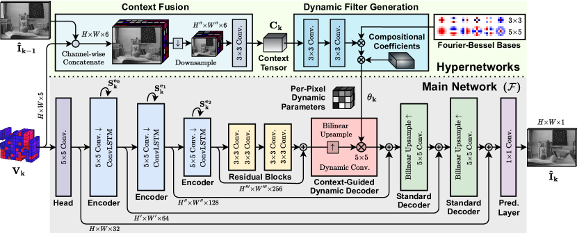
Figure 3: Overview of our proposed HyperE2VID architecture. The main network $\mathcal{F}$ uses a U-Net like architecture to process an event voxel grid $V_{k}$ and predict the intensity image $\hat{I}_{k}$ at each time step $k$. It includes downsampling encoder blocks, upsampling decoder blocks, and skip connections. The encoders incorporate ConvLSTM blocks to capture long temporal dependencies in the sparse event stream. The parameters of the context-guided dynamic decoder (CGDD) block are generated dynamically at inference time, enabling the network to adapt to highly varying event data. These parameters are generated via hypernetworks, consisting of a context fusion (CF) block and a dynamic filter generation (DFG) block. The DFG block employs two filter decomposition steps using multiscale Fourier-Bessel Bases and learned compositional coefficients, avoiding the high computational cost of per-pixel adaptive filters. The CF block fuses event features from the current time step $k$ with reconstructed image features from the previous time step $k-1$ to generate a context tensor. This fusion scheme combines the dynamic and static parts of the scene captured by events and images, respectively, to generate a context tensor that better represents the overall scene.

After representing each event group with a voxel grid, our task is to generate an image stream from the sequence of voxel grids. We use a recurrent neural network that consumes a voxel grid $V_{k}$ at each time step $k\in\left\{1,\ldots,{N_{I}}\right\}$, and generates an image $\hat{I}_{k}$ for that time step. Specifically, we use a U-Net [55] based fully convolutional architecture with recurrent encoder blocks, decoder blocks, and skip connections between them, similar to the E2VID model [7] and the subsequent works of [27], [8], and [10]. Then, we augment this main architecture with hypernetworks, dynamic convolutions, and a context fusion module. We refer to the resulting architecture as HyperE2VID.

Fig. 3 shows an overview of the proposed HyperE2VID framework. Our model consists of a main network $\mathcal{F}$ and hypernetworks that generate parameters for the dynamic part of the main network. From its input to output, the network $\mathcal{F}$ consists of one head layer, three recurrent encoder blocks, two residual blocks, one context-guided dynamic decoder (CGDD) block, two standard decoder blocks, and a prediction layer. The dynamic filter generation (DFG) block and the context fusion (CF) block act as hypernetworks that generate pixel-wise dynamic filter parameters for the dynamic part of the main network, i.e. the context-guided dynamic decoder block.

More formally, let $S_{k}$ be the recurrent state of the network for a time step $k$, containing states $\mathbf{S^{e_{n}}_{k}}$ of the three encoder blocks, where $n\in\{0,1,2\}$. Given the states from the previous time step, $S_{k-1}$, and the event voxel grid from the current time step, $V_{k}$, the main network $\mathcal{F}$ calculates the current states $S_{k}$ and predicts the intensity image $\hat{I}_{k}$ as follows:

$$(\hat{I}_{k},S_{k})=\mathcal{F}(V_{k},S_{k-1},\theta_{k})$$ (4)

with $\theta_{k}$ denoting the parameters of the convolutional layer at the CGDD block, which are generated dynamically at inference time by the DFG block, as below:

$$C_{k} =\text{CF}(V_{k},\hat{I}_{k-1})$$ (5)

$$\theta_{k} =\text{DFG}(C_{k})$$ (6)

To generate the parameters of the dynamic decoder, we use both the current event voxel grid $V_{k}$ and the previous reconstruction result $\hat{I}_{k-1}$. The context fusion (CF) block fuses these inputs to generate a context tensor $C_{k}$, which is then used as input to the dynamic filter generation block, DFG. This approach is motivated by the complementary nature of the two domains. Intensity images are better at capturing static parts of the scene but suffer in dynamic parts due to motion blur. In contrast, events are better suited for capturing fast motion due to their high temporal resolution but cannot capture static parts of the scene. By fusing $V_{k}$ and $\hat{I}_{k-1}$, the context tensor $C_{k}$ incorporates useful features that better describe both the static and dynamic parts of the scene.

Skip connections carry output feature maps of the head layer and each encoder block to the inputs of the respective symmetric decoder components, i.e. before each decoder block and the prediction layer. Element-wise summation is performed for these skip connections. ReLU activations are used for each convolutional layer unless specified otherwise. We describe each component of our architecture in more detail below:

Head layer. The head layer consists of a convolutional layer that has a kernel size of 5. The convolutional layer processes the event voxel grid with 5 temporal channels and outputs a tensor with 32 channels, while the spatial dimensions $H$ and $W$ of the input are maintained.

Encoder blocks. Each encoder block consists of a convolutional layer followed by a ConvLSTM [56]. The convolutional layer has a kernel size of 5 and stride of 2, thus it reduces the spatial dimensions of the input feature map by half. On the other hand, it doubles the number of channels. The ConvLSTM has a kernel size of 3 and maintains the spatial and channel dimensions of its inputs and internal states.

Residual blocks. Each residual block in our network comprises two convolutional layers with a kernel size of 3 that preserve the input’s spatial and channel dimensions. A skip connection adds the input features to the output features of the second convolution before the activation function.

Context-Guided Dynamic Decoder (CGDD) block. The context-guided dynamic decoder block includes bilinear upsampling to increase the spatial dimensions, followed by a dynamic convolutional layer. The convolution contains $5\times 5$ kernels and reduces the channel size by half. The parameters $\theta_{k}$ of this convolution are generated dynamically during inference time by the DFG block.

It is important to emphasize that all dynamic parameters are generated pixel-wise in that there exists a separate convolutional kernel for each pixel. This spatial adaptation is motivated by the fact that the pixels of an event camera work independently from each other. When there is more motion in one part of the scene, events are generated at a higher rate at corresponding pixels and the resulting voxel grid is denser in those regions. Our design enables the network to learn and use different filters for each part of the scene according to different motion patterns and event rates, making it more effective to process the event voxel grid with spatially varying densities.

Standard Decoder blocks. Each standard decoder block consists of bilinear upsampling followed by a standard convolutional layer. The details are the same as the context-guided dynamic decoder, except that the parameters are learned at training time and fixed at inference time.

Prediction layer. The prediction layer is a standard convolutional layer with a kernel size of 1 and it outputs the final predicted intensity image with 1 channel. We do not use an activation function after this layer.

Dynamic Filter Generation (DFG) block. A crucial component of our method is the dynamic filter generation. This block consumes a context tensor and output parameters for the CGDD block. The context tensor $C_{k}$ is expected to be at the same spatial size as the input of the dynamic convolution ($W^{\prime\prime}\times H^{\prime\prime}$). To generate the context tensor, we use a context fusion mechanism that fuses features from the event voxel grid ($V_{k}$) and the previous reconstruction ($\hat{I}_{k-1}$) of the network.

To reduce the computational cost, we use two filter decomposition steps while generating per-pixel dynamic filters. First, we decompose filters into per-pixel filter atoms generated dynamically. Second, we further decompose each filter atom into pre-fixed multi-scale Fourier-Bessel bases. Inspired by ACDA [14], our approach generates efficient per-pixel dynamic convolutions that vary spatially. However, unlike ACDA, our network architecture performs dynamic parameter generation independently through hypernetworks, which are guided by a context tensor designed to provide task-specific features for event-based video reconstruction.

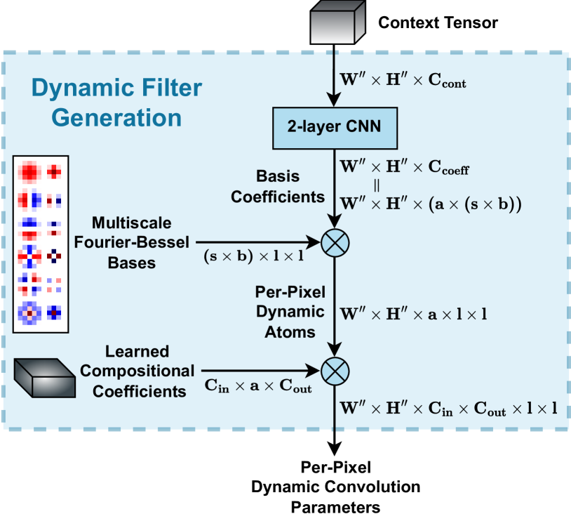
Figure 4: Dynamic Filter Generation (DFG) block. DFG block takes a context tensor as input and generates per-pixel dynamic convolution parameters via two filter decomposition steps, making use of pre-fixed multiscale Fourier-Bessel bases and learned compositional coefficients. More details are given in Section 3.

Fig. 4 illustrates the detailed operations of our proposed DFG block. A context tensor with dimensions $W^{\prime\prime}\times H^{\prime\prime}\times C_{\textit{cont}}$ is fed into a 2-layer CNN, producing pixelwise basis coefficients of size $C_{\textit{coeff}}$ that are used to generate per-pixel dynamic atoms via pre-fixed multiscale Fourier-Bessel bases. These bases are represented by a tensor of size $s\times b\times l\times l$, where $s$ is the number of scales, $b$ is the number of Fourier-Bessel bases at each scale, and $l$ is the kernel size for which the dynamic parameters are being generated. Multiplying the multiscale Fourier-Bessel bases with the basis coefficients generate per-pixel dynamic atoms of size $l\times l$. Number of generated atoms for each pixel is $a$, so it is possible to represent all of the generated atoms by a tensor of size $W^{\prime\prime}\times H^{\prime\prime}\times a\times l\times l$. Next, the compositional coefficients tensor of size $C_{\textit{in}}\times a\times C_{\textit{out}}$ is multiplied with these per-pixel dynamic atoms. These learned coefficients are fixed at inference time and shared across spatial positions. This multiplication produces a tensor of size $W^{\prime}\times H^{\prime}\times C_{\textit{in}}\times C_{\textit{out}}\times l\times l$, which serves as the parameters for the per-pixel dynamic convolution. Here, $C_{\textit{in}}$ and $C_{\textit{out}}$ are the number of input and output channels for the dynamic convolution, respectively. For the DFG block, we set $a=6$, $b=6$, and $l=5$. The number of scales $s=2$, meaning that we use $3\times 3$ and $5\times 5$ sized Fourier-Bessel bases. Since we have $b=6$ bases at each scale, we have a total of $s\times b=12$ Fourier-Bessel bases. The 2-layer CNN has a hidden channel size of 64. Both convolutional layers have a kernel size of 3, and they are followed by a batch normalization [57] layer and a tanh activation. The output of the CNN has $C_{\textit{coeff}}=a\times b\times s=72$ channels, to produce a separate coefficient per dynamic atom and per Fourier-Bessel basis.

Context Fusion (CF) block. The events are generated asynchronously only when the intensity of a pixel changes, and therefore the resulting event voxel grid is a sparse tensor, incorporating information only from the changing parts of the scene. Our HyperE2VID architecture conditions the dynamic decoder block parameters with both the current event voxel grid $V_{k}$ and the previous network reconstruction $\hat{I}_{k-1}$. These two domains provide complementary information; the intensity image is better suited for static parts of the scene, while the events are better for dynamic parts. We use the CF block to fuse this information, enabling the network to focus on intensity images for static parts and events for dynamic parts. Our context fusion block design concatenates $V_{k}$ and $\hat{I}_{k-1}$ channel-wise to form a 6-channel tensor. We downsample this tensor to match the input dimensions of the dynamic convolution at the CGDD block and then use a $3\times 3$ convolution to produce a context tensor with 32 channels. While more complex architectures are possible, we opt for a simple design for the context fusion block.

III-D Training Details

During training, we employ the following loss functions:

Perceptual Reconstruction Loss. We use the AlexNet [58] variant of the learned perceptual image patch similarity (LPIPS) [26] to enforce reconstructed images to be perceptually close to ground truth intensity images. LPIPS works by passing the predicted and reference images through a deep neural network architecture that was trained for visual recognition tasks, and using the distance between deep features from multiple layers of that network as a measure of the perceptual difference between the two images.

$$\mathcal{L}^{\text{LPIPS}}_{k}=\text{LPIPS}(\hat{I}_{k},I_{k})$$ (7)

Temporal Consistency Loss. We use the short-term temporal loss of [28], as employed in [27], to enforce temporal consistency between the images that are reconstructed in consecutive time steps of the network. This loss works by warping the previously reconstructed image using a ground truth optical flow to align it with the current reconstruction and using a masked distance between these aligned images as a measure of temporal consistency, where the mask is calculated from the warping error between the previous and the current ground truth intensity images. More formally, the temporal consistency loss is calculated as:

$$\mathcal{L}^{\text{TC}}_{k}=M_{k}\lVert\hat{I}_{k}-W(\hat{I}_{k-1},F_{k\rightarrow k-1})\lVert_{1}$$ (8)

where $F_{k\rightarrow k-1}$ denotes the optical flow map between time steps $k$ and $k-1$, $W$ is the warping function, and $M_{k}$ represents the occlusion mask which is computed as:

$$M_{k}=\text{exp}(-\alpha\lVert{I}_{k}-W({I}_{k-1},F_{k\rightarrow k-1})\lVert^{2}_{2})$$ (9)

where we use $\alpha=50$ as in [28, 27]. The mask $M_{k}$ contains smaller terms for pixels where the warping error between consecutive ground truth images is high, and therefore the masking operation effectively discards these pixels from the temporal consistency calculation of reconstructed frames.

The final loss for a time step $k$ is the sum of the perceptual reconstruction and temporal losses:

$$\mathcal{L}_{k}=\mathcal{L}^{\text{LPIPS}}_{k}+\mathcal{L}^{\text{TC}}_{k}$$ (10)

During training, we calculate the loss $\mathcal{L}_{k}$ at every $T_{S}$ time-steps in a training sequence, and the gradients of this loss with respect to the network parameters are calculated using the Truncated Back-propagation Through Time (TBPTT) algorithm [59] with a truncation period of $T_{T}$ time-steps. Setting $T_{S}>1$ and $T_{T}<k$ reduces memory requirements and speeds up the training process.

We implement our network in PyTorch [60]. We train the recurrent network with sequences of length 40, with the network parameters initialized using He initialization [61]. At the first time step of each sequence, the initial values of the previous reconstruction, $\hat{I}_{0}$, and the network states, $S_{0}$, are set to zero tensors. The loss calculation and the truncation periods are set as $T_{S}=10$ and $T_{T}=5$, respectively. We train our network for 400 epochs using a batch size of 10 and the AMSGrad [62] variant of the Adam [63] optimizer with a learning rate of 0.001. To track our trainings and experimental analyses, we used Weights & Biases [64].

At the start of the training, the previous reconstruction $\hat{I}_{k-1}$ of the network which is used for context fusion is far from optimal. This makes it harder for the context fusion block to learn useful representations, especially in the earlier epochs of the training. To resolve this issue, we employ a curriculum learning [65] strategy during the training. We start the training by using the ground-truth previous image $I_{k-1}$ instead of the previous reconstruction of the network $\hat{I}_{k-1}$ for context fusion. For the first 100 epochs, we gradually switch to using images that the network reconstructs at the previous time-step, by weighted averaging them with ground-truth images. After the 100th epoch, we continue the training by only using previous reconstructions for context fusion. Therefore, we use a modified version of Equation 5 during training:

$$\beta =\min(1,~{}\frac{\textit{epoch}}{100})$$ (11)

$$I_{\textit{context}} =\beta\cdot\hat{I}_{k-1}+(1-\beta)\cdot I_{k-1}$$ (12)

$$C_{k} =\text{CF}(V_{k},I_{\textit{context}})$$ (13)

This curriculum learning strategy allows the parameters of the hypernetworks to be learned more robustly, enabling the training process to converge to a better-performing model.

During training, we augment the images and event tensors with random crops and random flips as suggested in [27]. The size of random crops is $112\times 112$ and the probability of vertical and horizontal flips are both 0.5. Furthermore, we employ dynamic train-time noise augmentation, pause augmentation, and hot-pixel augmentation as described in [8].

IV Experimental Analysis

IV-A Training Dataset

We generate a synthetic training set as described in [8], using the multi objects 2D renderer option of ESIM [25] where multiple moving objects are captured with a camera restricted to 2D motion. The dataset consists of 280 sequences all of which are 10 secs in length. The contrast threshold values for event generation are in the range of 0.1 to 1.5. Each sequence includes generated event streams together with ground truth intensity images and optical flow maps with an average rate of 51 Hz. The resolutions of event and frame cameras are both $256\times 256$. The sequences include scenes containing up to 30 foreground objects with varying speeds and trajectories, where the objects are randomly selected images from the MS-COCO dataset [66].

IV-B Testing Datasets

To evaluate our method, we utilize sequences from three real-world datasets, namely the Event Camera Dataset (ECD) [67], the Multi Vehicle Stereo Event Camera (MVSEC) dataset [68] and the High-Quality Frames (HQF) dataset [8].

Event Camera Dataset (ECD). This dataset is captured by a DAVIS240C sensor [69] where events and frames are generated from the same pixel array of $240\times 180$ resolution. Following the common practice established by Rebecq et al. [27], we use seven short sequences from this dataset, where the camera moves with 6-DOF and with increasing speed in six of them. These sequences mostly contain simple office environments with static objects. The ground truth intensity frames are available at an average rate of 22 Hz, and we exclude scores from the initial few seconds of each sequence to align with prior work. Additionally, we exclude the parts of the sequences that contain motion blur due to fast camera motion while evaluating with full-reference metrics. In total, we use 1853 ground truth frames for full-reference metrics, and the specific start and end times of evaluation intervals are provided in [8]. We report these evaluation scores under the name ECD in our quantitative results tables. To assess the quality of the reconstructions under fast camera motion, we conduct a separate evaluation using the latter parts of the ECD sequences and a no-reference metric. It comprises a total of 4453 reconstructed frames, and its purpose is to examine the reconstruction quality when the camera moves rapidly. We report the scores from this evaluation under the name FAST in the quantitative results tables.

Multi Vehicle Stereo Event Camera (MVSEC) dataset. This dataset has longer sequences of indoor and outdoor environments, captured by a pair of DAVIS 346B cameras. These cameras generate events and frames from the same pixel array which has a resolution of $346\times 260$. We use the data from the left DAVIS camera in our experiments. Following [8], we also use specific time intervals of 6 sequences. Four of them are indoor sequences that are taken from a flying hexacopter, while the two outdoor sequences are taken from a vehicle driving in daylight. The average rate of ground truth intensity frames is around 30 Hz for indoor sequences and 45 Hz for outdoor sequences. The specific start and end times of evaluation intervals are given at [8]. The total number of ground truth frames used for evaluation is 11312. We report these scores under the name MVSEC in quantitative results tables. To assess the quality of our reconstruction method in low light conditions, we evaluate it on three night driving sequences from the MVSEC dataset using a no-reference metric. This evaluation comprises a total of 9415 reconstructed frames, with an average rate of 10 Hz. The scores from this evaluation are reported under the name NIGHT in the quantitative results tables.

High Quality Frames (HQF) dataset. This dataset has 14 indoor and outdoor image sequences that cover a diverse range of motions. The data is captured by two different DAVIS240C cameras with varying noise and contrast threshold characteristics. Both cameras generate events and frames from the same $240\times 180$ pixel array. The camera parameters and scenes are carefully selected to ensure that the ground truth frames are well-exposed and minimally motion-blurred. The dataset provides ground truth intensity frames with an average rate of 22.5 Hz, and following [8] we use the entire sequences for evaluation. In total, we use 15498 ground truth frames for this evaluation.

IV-C Evaluation Metrics

We evaluate the methods using three full-reference evaluation metrics, mean squared error (MSE), structural similarity (SSIM) [70], and learned perceptual image patch similarity (LPIPS) [26] when high-quality, distortion-free ground truth frames are available. To assess image quality under challenging scenarios, such as low light and fast motion, where ground truth frames are of low quality, we use a no-reference metric, BRISQUE [71]. These metrics have some settings that affect their results, and thus we provide the settings we use below:

MSE. Mean squared error is a standard metric without parameters. The only thing that can affect the result of MSE while comparing two images is the range of pixel values that images have. We use floating point pixel values in the range $[0,1]$ to calculate MSE. Lower MSE scores are better.

SSIM. For structural similarity we use the implementation from the scikit-image library [72], v0.19.3. We adjusted the parameters to use the Gaussian weighting scheme described in the original paper [70]. Similar to MSE, we input images with floating point pixel values in the range $[0,1]$ to SSIM calculation. Higher SSIM scores are better.

LPIPS. For LPIPS [26] we use v0.1.4 of the official implementation with pre-trained AlexNet [58] network. As required by the implementation, we normalize the images so that their pixel values are in the range $[-1,1]$. Lower LPIPS scores are better.

BRISQUE. For BRISQUE [71], we use the implementation in IQA-PyTorch toolbox [73], v0.1.5, with default settings. The implementation supports 3-channel RGB images, thus, we convert intensity images into RGB images by concatenating three copies of the grayscale image along the third dimension before calculating the scores. The pixel values are again in the range of $[0,1]$. Lower BRISQUE scores are better.

IV-D Competing Approaches

We compare our method against seven other methods from the literature, which are E2VID [27], FireNet [29], FireNet+ and E2VID+ [8], SPADE-E2VID [10], SSL-E2VID [34], and ET-Net [9]. E2VID+ and SSL-E2VID use the same network architecture as E2VID, but their training details are different. Similarly, FireNet+ uses the same network architecture as FireNet. We use the pre-trained models that the respective authors publicly share for each of these methods, and evaluate them using the same datasets and under the same settings. All of these methods use the same voxel-grid event representation as ours (Section III-B). We group events that have timestamps between every two consecutive ground truth frames and form the voxel grids using these. We also apply any pre-processing and post-processing steps when required by the method, such as the event tensor normalization and robust min/max normalization of E2VID. After generating reconstructions for each method, we perform quantitative analysis using the full-reference metrics, MSE, SSIM, and LPIPS, or the no-reference metric BRISQUE, depending on whether high-quality ground truth frames are available or not. We do not perform histogram equalization to reconstructions or ground truth images before calculating evaluation metrics. The quantitative results as well as the qualitative analysis are given in Section IV-E. We also compare the computational complexity of each network architecture in Section IV-G.

IV-E Experimental Results

TABLE I: Quantitative results of existing methods and our proposed method on sequences from ECD, MVSEC, and HQF datasets.

		ECD				MVSEC				HQF				FAST		NIGHT
		MSE $\downarrow$	SSIM $\uparrow$	LPIPS $\downarrow$		MSE $\downarrow$	SSIM $\uparrow$	LPIPS $\downarrow$		MSE $\downarrow$	SSIM $\uparrow$	LPIPS $\downarrow$	BRISQUE $\downarrow$
E2VID [27]		0.212	0.424	0.350		0.337	0.206	0.705		0.127	0.540	0.382		14.729		8.793
FireNet [29]		0.131	0.502	0.320		0.292	0.261	0.700		0.094	0.533	0.441		19.957		21.311
E2VID+ [8]		0.070	0.560	0.236		0.132	0.345	0.514		0.036	0.643	0.252		22.627		12.285
FireNet+ [8]		0.063	0.555	0.290		0.218	0.297	0.570		0.040	0.614	0.314		18.399		10.019
SPADE-E2VID [10]		0.091	0.517	0.337		0.138	0.342	0.589		0.077	0.521	0.502		18.925		24.011
SSL-E2VID [34]		0.046	0.364	0.425		0.062	0.345	0.593		0.126	0.295	0.498		60.523		63.847
ET-Net [9]		0.047	0.617	0.224		0.107	0.380	0.489		0.032	0.658	0.260		19.698		15.533
HyperE2VID (ours)		0.033	0.655	0.212		0.076	0.419	0.476		0.031	0.658	0.257		14.024		5.973

boxes_6dof
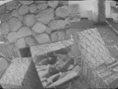
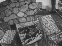
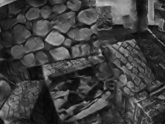
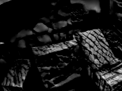
office_zigz.
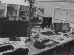
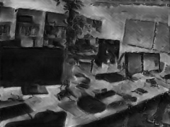
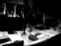
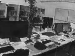
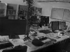
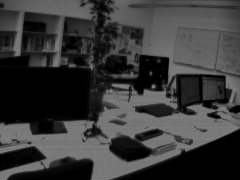
indoor_fly2
out_day2
desk_fast
high_text.
still_life
dynamic
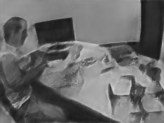
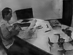
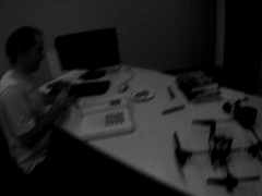
out_night1
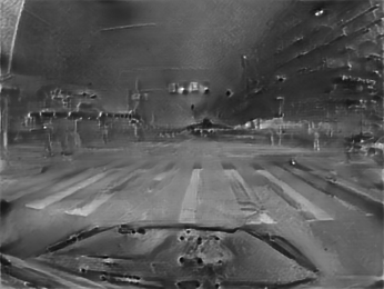
	E2VID	E2VID+	FireNet+	SSL-E2VID	ET-Net	HyperE2VID	Ground Truth

Figure 5: Qualitative comparisons on some sequences from ECD (rows 1-2), MVSEC (rows 3-4), HQF (rows 5-7), FAST (row 8) and NIGHT (row 9). While the competing approaches suffer from low contrast, blur, and extensive artifacts, HyperE2VID reconstructions have high contrast and preserve sharp details around the edges, with minimal artifacts in textureless regions.

Table I presents the quantitative results obtained from evaluating the methods on sequences from the aforementioned datasets. We calculated the average values of each metric across all evaluated frames. The HyperE2VID method achieves state-of-the-art performance in terms of most metrics. On the ECD and MVSEC datasets, it outperforms the second-best method, ET-Net, by a large margin. On the HQF dataset, it delivers results on par with or slightly better than existing approaches. In challenging scenarios involving fast camera motion (FAST) or night driving (NIGHT), it obtains the best BRISQUE scores, surpassing the second-best method, E2VID. These results demonstrate the effectiveness of the proposed HyperE2VID method, which generates perceptually more pleasing and high-fidelity reconstructions.

We present qualitative results for ECD, MVSEC, and HQF datasets in Fig. 5. We omit reconstructions of FireNet and SPADE-E2VID due to lower quantitative scores and focus on the performances of E2VID, E2VID+, FireNet+, E2VID+, SSL-E2VID, ET-Net, and HyperE2VID. Sample scenes are shown from ECD (rows 1,2), MVSEC (rows 3,4), and HQF (rows 5-7) datasets, as well as fast parts of ECD (FAST, row 8) and night sequences of MVSEC (NIGHT, row 9) datasets. Each row show reconstructions of each model (first 6 columns) with the groundtruth frame given in the rightmost column.

The visual qualities of reconstructions are mostly in line with the quantitative results. Among the six methods, FireNet+ and SSL-E2VID tend to have the lowest quality with prominent visual artifacts and overly dark regions. Reconstructions of E2VID+ have lesser artifacts, especially at scenes from the HQF dataset. E2VID+ also produces nice-looking images for the outdoor scenes of the MVSEC dataset. However, its reconstructions are generally of low contrast and blurry around the edges. ET-Net has better contrast but has more artifacts at textureless regions and around the edges of objects. The reconstructions of HyperE2VID are of high contrast and sharp around the edges. Moreover, the textureless regions are mostly reconstructed with lesser artifacts.

IV-F Ablation Study

TABLE II: Ablation results of HyperE2VID variants where we alter the context information, the existence of convolutional context fusion (CF) block, and curriculum learning (CL) strategy.

				ECD				MVSEC				HQF				FAST		NIGHT
Context	CL	CF		MSE $\downarrow$	SSIM $\uparrow$	LPIPS $\downarrow$		MSE $\downarrow$	SSIM $\uparrow$	LPIPS $\downarrow$		MSE $\downarrow$	SSIM $\uparrow$	LPIPS $\downarrow$	BRISQUE $\downarrow$
EV				0.048	0.609	0.219		0.189	0.311	0.549		0.050	0.620	0.280		13.415		1.045
IM				0.050	0.608	0.229		0.181	0.302	0.573		0.035	0.640	0.276		18.791		10.124
EV+IM				0.039	0.630	0.212		0.152	0.342	0.532		0.036	0.642	0.271		18.638		9.212
EV+IM		✓		0.044	0.619	0.218		0.113	0.363	0.516		0.039	0.636	0.266		17.728		7.375
EV+IM	✓			0.038	0.625	0.216		0.120	0.355	0.506		0.032	0.657	0.259		18.241		6.085
EV+IM	✓	✓		0.033	0.655	0.212		0.076	0.419	0.476		0.031	0.658	0.257		14.024		5.973

We conduct ablation studies to analyze the effectiveness of various design choices, including the context information used. Specifically, we investigate hypernetworks that use only event context, only image context, or both event and image context, denoted as EV, IM, and EV+IM, respectively. For EV+IM, we also examine the impact of using the curriculum learning strategy (CL) and convolutional context fusion (CF). When CF is not used, we concatenate the image and event tensors channel-wise, and downsample the resulting tensor to match the input of the dynamic convolution in the CGDD block. In our experiments, we investigate the impact of specific design choices while keeping all other training and evaluation settings unchanged. The results are summarized in Table II. Our findings reveal that leveraging both events and images as contextual information (EV+IM) generally outperforms using only events (EV) or only images (IM), with the exception of event-only context performing better on fast motion and night driving sequences. When using both events and images (EV+IM), incorporating only the context fusion (CF) yields performance improvement on the MVSEC dataset. Conversely, incorporating only the curriculum learning strategy (CL) enhances performance on both the MVSEC and HQF datasets. Combining all these components results in our proposed HyperE2VID model (last row), which achieves the best scores on ECD, MVSEC, and HQF datasets, and second-best scores on FAST and NIGHT datasets.

IV-G Computational Complexity

We also analyze the computational complexity of our method and compare it to other competing methods from the literature. We consider two computational metrics for this analysis: (1) the number of model parameters, and (2) inference time. The number of parameters is an important metric that indicates the memory requirements of the model, and the inference time is a direct indicator of the real-time performance of (the maximum frame-per-seconds that can be obtained with) the model. To measure inference time, we use data with a resolution of 240$\times$180, and report the average inference time in ms, on a workstation with Quadro RTX 5000 GPU. We present the results of these computational complexity metrics in Table III. Here, the numbers of model parameters are given in millions and the inference times are given in milliseconds. Methods that share a common network architecture are presented in the same row. Here, it can be seen that our method provides a good trade-off between accuracy and efficiency. HyperE2VID is a significantly smaller and faster network than ET-Net while generating reconstruction with better visual quality. On the other hand, the smallest and fastest methods, FireNet and FireNet+, generate reconstructions that have significantly lower visual quality.

TABLE III: Computational complexity of network architectures in terms of the number of model parameters in millions and inference time in milliseconds.

Network Architecture		Number of Params (M)	Inference Time (ms)
E2VID [27, 8, 34]		10.71	5.1
FireNet [29, 8]		0.04	1.6
SPADE-E2VID [10]		11.46	16.1
ET-Net [9]		22.18	32.1
HyperE2VID (ours)		10.15	6.6

V Conclusion

In this work, we presented HyperE2VID, a novel dynamic network architecture for event-based video reconstruction that improves the state-of-the-art by employing hypernetworks and dynamic convolutions. Our approach generates adaptive filters using hypernetworks, which are dynamically generated at inference time based on the scene context encoded via event voxel grids and previously reconstructed intensity images, and thus deals with static and dynamic parts of the scene more effectively. Experimental results on several challenging datasets show that HyperE2VID outperforms previous state-of-the-art methods in terms of visual quality while reducing memory consumption and inference time. Our work demonstrates the potential of dynamic network architectures and hypernetworks for processing highly varying event data, opening up possibilities for future research in this direction, targeting more tasks like event-based optical-flow estimation.

VI Acknowledgments

This work was supported in part by KUIS AI Research Award, TUBITAK-1001 Program Award No. 121E454, and BAGEP 2021 Award of the Science Academy to A. Erdem.

References

- [1] G. Gallego, T. Delbrück, G. Orchard, C. Bartolozzi, B. Taba, A. Censi, S. Leutenegger, A. J. Davison, J. Conradt, K. Daniilidis et al., “Event-based vision: A survey,” IEEE Trans. Pattern Anal. Mach. Intell., vol. 44, no. 1, pp. 154–180, 2020.
- [2] J. Li, J. Li, L. Zhu, X. Xiang, T. Huang, and Y. Tian, “Asynchronous spatio-temporal memory network for continuous event-based object detection,” IEEE Trans. Image Process., vol. 31, pp. 2975–2987, 2022.
- [3] Z. Jia, K. You, W. He, Y. Tian, Y. Feng, Y. Wang, X. Jia, Y. Lou, J. Zhang, G. Li et al., “Event-based semantic segmentation with posterior attention,” IEEE Trans. Image Process., 2023.
- [4] G. Chen, S. Qu, Z. Li, H. Zhu, J. Dong, M. Liu, and J. Conradt, “Neuromorphic vision-based fall localization in event streams with temporal–spatial attention weighted network,” IEEE Trans. Cybern., vol. 52, no. 9, pp. 9251–9262, 2022.
- [5] B. Forrai, T. Miki, D. Gehrig, M. Hutter, and D. Scaramuzza, “Event-based agile object catching with a quadrupedal robot,” arXiv preprint arXiv:2303.17479, 2023.
- [6] J. P. Rodríguez-Gómez, R. Tapia, M. d. M. G. Garcia, J. R. Martínez-de Dios, and A. Ollero, “Free as a bird: Event-based dynamic sense-and-avoid for ornithopter robot flight,” IEEE Robot. Autom. Lett., vol. 7, no. 2, pp. 5413–5420, 2022.
- [7] H. Rebecq, R. Ranftl, V. Koltun, and D. Scaramuzza, “Events-to-video: Bringing modern computer vision to event cameras,” in CVPR, 2019, pp. 3857–3866.
- [8] T. Stoffregen, C. Scheerlinck, D. Scaramuzza, T. Drummond, N. Barnes, L. Kleeman, and R. Mahony, “Reducing the sim-to-real gap for event cameras,” in ECCV, 2020.
- [9] W. Weng, Y. Zhang, and Z. Xiong, “Event-based video reconstruction using transformer,” in ICCV, 2021, pp. 2563–2572.
- [10] P. R. G. Cadena, Y. Qian, C. Wang, and M. Yang, “SPADE-E2VID: Spatially-adaptive denormalization for event-based video reconstruction,” IEEE Trans. Image Process., vol. 30, pp. 2488–2500, 2021.
- [11] A. Vaswani, N. Shazeer, N. Parmar, J. Uszkoreit, L. Jones, A. N. Gomez, Ł. Kaiser, and I. Polosukhin, “Attention is all you need,” in NeurIPS, 2017, pp. 5998–6008.
- [12] D. Ha, A. Dai, and Q. V. Le, “Hypernetworks,” arXiv preprint arXiv:1609.09106, 2016.
- [13] Y. Han, G. Huang, S. Song, L. Yang, H. Wang, and Y. Wang, “Dynamic neural networks: A survey,” IEEE Trans. Pattern Anal. Mach. Intell., 2021.
- [14] Z. Wang, Z. Miao, J. Hu, and Q. Qiu, “Adaptive convolutions with per-pixel dynamic filter atom,” in ICCV, 2021, pp. 12 302–12 311.
- [15] M. Cook, L. Gugelmann, F. Jug, C. Krautz, and A. Steger, “Interacting maps for fast visual interpretation,” in IJCNN, 2011, pp. 770–776.
- [16] H. Kim, A. Handa, R. Benosman, S. Ieng, and A. Davison, “Simultaneous mosaicing and tracking with an event camera,” in BMVC, 2014.
- [17] A. Agrawal, R. Chellappa, and R. Raskar, “An algebraic approach to surface reconstruction from gradient fields,” in ICCV, vol. 1, 2005, pp. 174–181.
- [18] H. Kim, S. Leutenegger, and A. J. Davison, “Real-time 3d reconstruction and 6-dof tracking with an event camera,” in ECCV, 2016, pp. 349–364.
- [19] S. Barua, Y. Miyatani, and A. Veeraraghavan, “Direct face detection and video reconstruction from event cameras,” in WACV, 2016, pp. 1–9.
- [20] M. Aharon, M. Elad, and A. Bruckstein, “K-SVD: An algorithm for designing overcomplete dictionaries for sparse representation,” IEEE Transactions on signal processing, vol. 54, no. 11, pp. 4311–4322, 2006.
- [21] P. Bardow, A. J. Davison, and S. Leutenegger, “Simultaneous optical flow and intensity estimation from an event camera,” in CVPR, 2016, pp. 884–892.
- [22] G. Munda, C. Reinbacher, and T. Pock, “Real-time intensity-image reconstruction for event cameras using manifold regularisation,” Int. J. Comput. Vis., vol. 126, no. 12, pp. 1381–1393, 2018.
- [23] C. Scheerlinck, N. Barnes, and R. Mahony, “Continuous-time intensity estimation using event cameras,” in ACCV, December 2018, pp. 308–324. [Online]. Available: https://cedric-scheerlinck.github.io/files/2018_scheerlinck_continuous-time_intensity_estimation.pdf
- [24] L. Wang, S. M. Mostafavi, Y.-S. Ho, K.-J. Yoon et al., “Event-based high dynamic range image and very high frame rate video generation using conditional generative adversarial networks,” in CVPR, 2019, pp. 10 081–10 090.
- [25] H. Rebecq, D. Gehrig, and D. Scaramuzza, “ESIM: an open event camera simulator,” in CoRL, 2018, pp. 969–982.
- [26] R. Zhang, P. Isola, A. A. Efros, E. Shechtman, and O. Wang, “The unreasonable effectiveness of deep features as a perceptual metric,” in CVPR, 2018, pp. 586–595.
- [27] H. Rebecq, R. Ranftl, V. Koltun, and D. Scaramuzza, “High speed and high dynamic range video with an event camera,” IEEE Trans. Pattern Anal. Mach. Intell., 2019.
- [28] W.-S. Lai, J.-B. Huang, O. Wang, E. Shechtman, E. Yumer, and M.-H. Yang, “Learning blind video temporal consistency,” in ECCV, 2018, pp. 170–185.
- [29] C. Scheerlinck, H. Rebecq, D. Gehrig, N. Barnes, R. Mahony, and D. Scaramuzza, “Fast image reconstruction with an event camera,” in WACV, 2020, pp. 156–163.
- [30] S. Zhang, Y. Zhang, Z. Jiang, D. Zou, J. Ren, and B. Zhou, “Learning to see in the dark with events,” in ECCV, vol. 1, 2020, p. 2.
- [31] T. Park, M.-Y. Liu, T.-C. Wang, and J.-Y. Zhu, “Semantic image synthesis with spatially-adaptive normalization,” in CVPR, 2019, pp. 2337–2346.
- [32] S. M. Mostafavi, J. Choi, and K.-J. Yoon, “Learning to super resolve intensity images from events,” in CVPR, 2020, pp. 2768–2776.
- [33] L. Wang, T.-K. Kim, and K.-J. Yoon, “EventSR: From asynchronous events to image reconstruction, restoration, and super-resolution via end-to-end adversarial learning,” in CVPR, 2020, pp. 8315–8325.
- [34] F. Paredes-Vallés and G. C. de Croon, “Back to event basics: Self-supervised learning of image reconstruction for event cameras via photometric constancy,” in CVPR, 2021, pp. 3446–3455.
- [35] G. Gallego, C. Forster, E. Mueggler, and D. Scaramuzza, “Event-based camera pose tracking using a generative event model,” arXiv preprint arXiv:1510.01972, 2015.
- [36] Y. Zou, Y. Zheng, T. Takatani, and Y. Fu, “Learning to reconstruct high speed and high dynamic range videos from events,” in CVPR, 2021, pp. 2024–2033.
- [37] L. Zhu, X. Wang, Y. Chang, J. Li, T. Huang, and Y. Tian, “Event-based video reconstruction via potential-assisted spiking neural network,” in CVPR, 2022, pp. 3594–3604.
- [38] Z. Zhang, A. Yezzi, and G. Gallego, “Formulating event-based image reconstruction as a linear inverse problem with deep regularization using optical flow,” IEEE Trans. Pattern Anal. Mach. Intell., no. 01, pp. 1–18, 2022.
- [39] X. Jia, B. De Brabandere, T. Tuytelaars, and L. V. Gool, “Dynamic filter networks,” NeurIPS, vol. 29, 2016.
- [40] Y. Nirkin, L. Wolf, and T. Hassner, “HyperSeg: Patch-wise hypernetwork for real-time semantic segmentation,” in CVPR, 2021, pp. 4061–4070.
- [41] T. R. Shaham, M. Gharbi, R. Zhang, E. Shechtman, and T. Michaeli, “Spatially-adaptive pixelwise networks for fast image translation,” in CVPR, 2021, pp. 14 882–14 891.
- [42] B. Yang, G. Bender, Q. V. Le, and J. Ngiam, “Condconv: Conditionally parameterized convolutions for efficient inference,” NeurIPS, vol. 32, 2019.
- [43] Y. Chen, X. Dai, M. Liu, D. Chen, L. Yuan, and Z. Liu, “Dynamic convolution: Attention over convolution kernels,” in CVPR, 2020, pp. 11 030–11 039.
- [44] H. Su, V. Jampani, D. Sun, O. Gallo, E. Learned-Miller, and J. Kautz, “Pixel-adaptive convolutional neural networks,” in CVPR, 2019, pp. 11 166–11 175.
- [45] J. Chen, X. Wang, Z. Guo, X. Zhang, and J. Sun, “Dynamic region-aware convolution,” in CVPR, 2021, pp. 8064–8073.
- [46] M. Abramowitz and I. A. Stegun, Handbook of mathematical functions with formulas, graphs, and mathematical tables. US Government printing office, 1964, vol. 55.
- [47] J. Dai, H. Qi, Y. Xiong, Y. Li, G. Zhang, H. Hu, and Y. Wei, “Deformable convolutional networks,” in ICCV, 2017, pp. 764–773.
- [48] J. Han, Y. Yang, C. Zhou, C. Xu, and B. Shi, “Evintsr-net: Event guided multiple latent frames reconstruction and super-resolution,” in ICCV, 2021, pp. 4882–4891.
- [49] N. Messikommer, S. Georgoulis, D. Gehrig, S. Tulyakov, J. Erbach, A. Bochicchio, Y. Li, and D. Scaramuzza, “Multi-bracket high dynamic range imaging with event cameras,” in CVPR, 2022, pp. 547–557.
- [50] P. Vitoria, S. Georgoulis, S. Tulyakov, A. Bochicchio, J. Erbach, and Y. Li, “Event-based image deblurring with dynamic motion awareness,” in ECCVW, 2023, pp. 95–112.
- [51] B. Xie, Y. Deng, Z. Shao, H. Liu, and Y. Li, “Vmv-gcn: Volumetric multi-view based graph cnn for event stream classification,” IEEE Robot. Autom. Lett., vol. 7, pp. 1976–1983, 2022.
- [52] Y. Jing, Y. Yang, X. Wang, M. Song, and D. Tao, “Turning frequency to resolution: Video super-resolution via event cameras,” in CVPR, 2021, pp. 7772–7781.
- [53] Z. Xiao, W. Weng, Y. Zhang, and Z. Xiong, “Eva2: Event-assisted video frame interpolation via cross-modal alignment and aggregation,” IEEE Trans. Comput. Imaging, vol. 8, pp. 1145–1158, 2022.
- [54] A. Zihao Zhu, L. Yuan, K. Chaney, and K. Daniilidis, “Unsupervised event-based optical flow using motion compensation,” in ECCV, 2018.
- [55] O. Ronneberger, P. Fischer, and T. Brox, “U-net: Convolutional networks for biomedical image segmentation,” in MICCAI, 2015, pp. 234–241.
- [56] X. Shi, Z. Chen, H. Wang, D.-Y. Yeung, W.-K. Wong, and W.-c. Woo, “Convolutional lstm network: A machine learning approach for precipitation nowcasting,” NeurIPS, vol. 28, pp. 802–810, 2015.
- [57] S. Ioffe and C. Szegedy, “Batch normalization: Accelerating deep network training by reducing internal covariate shift,” in ICML, 2015, pp. 448–456.
- [58] A. Krizhevsky, I. Sutskever, and G. E. Hinton, “Imagenet classification with deep convolutional neural networks,” Commun. ACM, vol. 60, no. 6, pp. 84–90, 2017.
- [59] R. J. Williams and J. Peng, “An efficient gradient-based algorithm for on-line training of recurrent network trajectories,” Neural computation, vol. 2, no. 4, pp. 490–501, 1990.
- [60] A. Paszke, S. Gross, F. Massa, A. Lerer, J. Bradbury, G. Chanan, T. Killeen, Z. Lin, N. Gimelshein, L. Antiga et al., “Pytorch: An imperative style, high-performance deep learning library,” NeurIPS, vol. 32, pp. 8026–8037, 2019.
- [61] K. He, X. Zhang, S. Ren, and J. Sun, “Delving deep into rectifiers: Surpassing human-level performance on imagenet classification,” in ICCV, 2015, pp. 1026–1034.
- [62] S. J. Reddi, S. Kale, and S. Kumar, “On the convergence of adam and beyond,” arXiv preprint arXiv:1904.09237, 2019.
- [63] D. P. Kingma and J. Ba, “Adam: A method for stochastic optimization,” arXiv preprint arXiv:1412.6980, 2014.
- [64] L. Biewald, “Experiment tracking with weights and biases,” 2020, software available from wandb.com. [Online]. Available: https://www.wandb.com/
- [65] Y. Bengio, J. Louradour, R. Collobert, and J. Weston, “Curriculum learning,” in ICML, 2009, pp. 41–48.
- [66] T.-Y. Lin, M. Maire, S. Belongie, J. Hays, P. Perona, D. Ramanan, P. Dollár, and C. L. Zitnick, “Microsoft COCO: Common objects in context,” in ECCV, 2014, pp. 740–755.
- [67] E. Mueggler, H. Rebecq, G. Gallego, T. Delbruck, and D. Scaramuzza, “The event-camera dataset and simulator: Event-based data for pose estimation, visual odometry, and slam,” Int. J. Robot. Res., vol. 36, no. 2, pp. 142–149, 2017.
- [68] A. Z. Zhu, D. Thakur, T. Özaslan, B. Pfrommer, V. Kumar, and K. Daniilidis, “The multivehicle stereo event camera dataset: An event camera dataset for 3d perception,” IEEE Robot. Autom. Lett., vol. 3, no. 3, pp. 2032–2039, 2018.
- [69] C. Brandli, R. Berner, M. Yang, S.-C. Liu, and T. Delbruck, “A 240 180 130 db 3 s latency global shutter spatiotemporal vision sensor,” IEEE J. Solid-State Circuits, vol. 49, no. 10, pp. 2333–2341, 2014.
- [70] Z. Wang, A. C. Bovik, H. R. Sheikh, and E. P. Simoncelli, “Image quality assessment: from error visibility to structural similarity,” IEEE Trans. Image Process., vol. 13, no. 4, pp. 600–612, 2004.
- [71] A. Mittal, A. K. Moorthy, and A. C. Bovik, “No-reference image quality assessment in the spatial domain,” IEEE Trans. Image Process., vol. 21, no. 12, pp. 4695–4708, 2012.
- [72] S. Van der Walt, J. L. Schönberger, J. Nunez-Iglesias, F. Boulogne, J. D. Warner, N. Yager, E. Gouillart, and T. Yu, “scikit-image: image processing in python,” PeerJ, vol. 2, p. e453, 2014.
- [73] C. Chen and J. Mo, “IQA-PyTorch: Pytorch toolbox for image quality assessment,” [Online]. Available: https://github.com/chaofengc/IQA-PyTorch, 2022.