Dynamic Graph Representation Learning for Depression Screening with Transformer

Abstract.

Early detection of mental disorder is crucial as it enables prompt intervention and treatment, which can greatly improve outcomes for individuals suffering from debilitating mental affliction. The recent proliferation of mental health discussions on social media platforms presents research opportunities to investigate mental health and potentially detect instances of mental illness. However, existing depression detection methods are constrained due to two major limitations: (1) the reliance on feature engineering and (2) the lack of consideration for time-varying factors. Specifically, these methods require extensive feature engineering and domain knowledge, which heavily rely on the amount, quality, and type of user-generated content. Moreover, these methods ignore the important impact of time-varying factors on depression detection, such as the dynamics of linguistic patterns and interpersonal interactive behaviors over time on social media (e.g., replies, mentions, and quote-tweets).

To tackle these limitations, we propose an early depression detection framework, ContrastEgo, that effectively learns multi-scale user latent representations (node-level and graph-level) by capturing the topological dynamics of users’ social interactions with their friends using attention mechanism. Specifically, ContrastEgo treats each user as a dynamic time-evolving attributed graph (ego-network) and leverages supervised contrastive learning to maximize the agreement of users’ representations at different scales while minimizing the agreement of users’ representations to differentiate between depressed and control groups. ContrastEgo embraces four modules, (1) constructing users’ heterogeneous interactive graphs, (2) extracting the representations of users’ interaction snapshots using graph neural networks, (3) modeling the sequences of snapshots using attention mechanism, and (4) depression detection using contrastive learning. Extensive experiments on Twitter data demonstrate that ContrastEgo significantly outperforms the state-of-the-art methods in terms of all the effectiveness metrics in various experimental settings. Compared to all baseline methods, ContrastEgo is able to effectively predict early depression in Twitter users with up to 5% and 4% improvement on F1 score and AUROC, respectively.

1. Introduction

Depression is a prevalent and pernicious global health issue that affects millions of people worldwide. The World Health Organization’s report (who, [n. d.]) stated that the cost to the global economy by depression and anxiety disorders was estimated to be one trillion dollars annually, primarily due to diminished productivity. This loss not only affects individuals and families, but also has far-reaching implications for society as a whole. Left untreated, depression can cause significant distress and impairments, leading to a range of severe complications such as suicide, substance abuse, absenteeism, reduced productivity, and other mental health disorders. Early detection and treatment of depression are crucial in avoiding the exacerbation of the condition. The prolongation of untreated depression can result in a manifestation that becomes increasingly severe and resistant. Despite the significance of early detection and treatment, fear of mental illness stigma often impedes individuals from seeking help, even in the face of debilitating symptoms, presenting a significant barrier to care. Consequently, identifying individuals at risk of developing depression and providing them with early intervention and support becomes more challenging. Fortunately, there has been a recent surge in individuals sharing their mental health experiences and openly discussing their mental health issues on social media platforms. This presents a valuable opportunity for researchers to gain insights into the mental health and well-being of individuals by leveraging user-generated content shared on these platforms. The effective analysis of social media data holds the potential to lead to early detection of individuals who may be at risk of developing depression.

Existing approaches and limitations. Studies in the detection of depression in social media are predominantly focused on the exploitation of text-based features. Several classical machine learning classification models have been utilized to predict depression from social media data, exhibiting reasonable accuracy. These methods include Naive Bayes Classifier (Chatterjee et al., 2021; Deshpande and Rao, 2017), Support Vector Machine (De Choudhury et al., 2021), and Logistic Regression (Shen et al., 2017; Preoţiuc-Pietro et al., 2015; Jiang et al., 2018). However, these approaches may be impeded by the need for copious amounts of data to train, and their ability to process large amounts of data may be inferior to that of deep learning-based methods. In contrast, deep learning-based techniques for depression detection leverage the advanced representation-learning capabilities of neural networks. These methods have been applied to capture complex patterns and relationships in social media data, including text, images, and social network structures, to predict depression. These techniques include using Convolutional Neural Networks (CNNs) (Yates et al., 2017; Husseini Orabi et al., 2018), Recurrent Neural Networks (RNNs) (Husseini Orabi et al., 2018), Long Short-Term Memory (LSTM) networks (Ghosh and Anwar, 2021; Shah et al., 2020), Gated Recurrent Unit (GRU) networks (Zogan et al., 2021), and Graph Neural Networks (GNNs) (Ivan et al., 2022). Prior studies  (Ghosh and Anwar, 2021; Shah et al., 2020; Husseini Orabi et al., 2018; Pirayesh et al., 2021; Ophir et al., 2020) have focused on the application of language or sentiment analysis to identify words or phrases commonly associated with depression, such as the presence of negative words or terms such as ”sad,” ”hopeless,” and ”worthless.” However, these prediction performances are highly contingent upon the quality and quantity of the data used, with explicit language usage being easier to predict than more subtle or indirect language usage. Additionally, collecting sufficient depression-related data to train domain-specific word embeddings can be challenging. Some recent studies have opted to leverage pretrained models (Figuerêdo et al., 2022; S and Antony, 2022) for the detection of depression. Recent studies (Pirayesh et al., 2021; Ivan et al., 2022; De Choudhury et al., 2021) have also emphasized the significance of social circles and their impacts on an individual’s mental state, highlighting the need for a more holistic approach to depression detection in social media.

Our observations and contributions. We make two important observations. First, the inability of existing solutions to support early depression detection is a serious limitation in practice. Existing depression detection methods heavily rely on the amount, quality, and type of user-generated content on social media, thus failing to deal with those depressed users with only limited social footprints. As a result, those methods tend to suffer from the cold-start problem and fail to detect depression effectively at an early stage. However, the early detection of depression plays a vital role in supporting healthcare professionals for determining timely and targeted interventions in a clinical setting.

Second, the prediction of the onset of psychiatric diseases (including mental depression) may benefit from treating each individual as a dynamic system with time-evolving structure and attributes (e.g., a dynamic graph consisting of multiple snapshots of clinical states). However, the existing depression detection methods fail to take into account the important impact of the time-varying factors on depression detection, such as the dynamics of the linguistic patterns and interpersonal interactive behaviors over time on social media.

In this paper, we propose an early depression detection framework, ContrastEgo, that effectively learns multi-scale user latent representations (node-level and graph-level) by capturing the topological dynamics of users’ social interactions with their friends using attention mechanism. Specifically, ContrastEgo treats each user as a dynamic time-evolving attributed graph (ego-network) and leverages supervised contrastive learning to differentiate between depressed and control groups. Our contributions can be summarized as follows:

1. ContrastEgo treats the dynamic nature of user interactions on social media as first-class citizens to detect depression at an early stage. To the best of our knowledge, ContrastEgo is among the first to consider the early detection of depression with temporal aspects. Our research findings emphasize the significance of pattern changes inherent in mental disorders and provide a novel and insightful viewpoint. This could result in a more efficient and effective early detection for individuals who may be at risk of mental illness for timely and targeted interventions.

2. In order to capture the interpersonal dynamics on social media to identify depression status, ContrastEgo utilizes graph neural networks to encode social interactions and extract the latent user representations for each snapshot at multiple scales (at the node level and the graph level).

3. In order to capture the temporal dynamics (e.g., abrupt versus gradual onset) of depression, ContrastEgo utilizes a transformer architecture to encode the sequences of snapshots using attention mechanism.

4. ContrastEgo adopts supervised contrastive learning (Khosla et al., 2020) to maximize the agreement of users’ representations extracted at different scales and minimize the agreement of users’ representations between the individuals with depression and those without depression.

5. Extensive experiments on real-world Twitter data verify that ContrastEgo consistently outperforms the state-of-the-art methods in various experimental settings. In particular, ContrastEgo has shown an improvement of up to 4% in the AUROC score for predicting early depression in Twitter users compared to the state-of-the-art methods.

The organization of this paper is as follows. In Section 2, we present background information. In Section 3, we provide an overview of ContrastEgo. In Section 4, we explain the building blocks of ContrastEgo. Section 5 compares the performance of ContrastEgo with that of the state-of-the-art methods. Section 6 reviews the related work while Section 7 concludes the paper.

2. Preliminaries

Graph snapshot. A graph snapshot $G_{t}=(V_{t},E_{t})$ is a representation of a graph at a specific point in time $t$, where $V$ is a set of vertices and $E$ is a set of edges connecting the vertices. In our model, a graph snapshot of a user $U$ represents a collection of interactions around $U$ within a specific time frame. The vertices in the graph $V$ correspond to the individuals involved in the interactions, and the edges $E$ represent the interactions between individuals and their friends. Each vertex is represented by a vector of tweet embeddings, and each edge represents a type of interaction and the time period of the interaction.

Dynamic Graph. A dynamic graph can be formally defined as a sequence of graph snapshots with changing topological structures $G_{1},G_{2},...,G_{T}$, where each snapshot $G_{t}=(V_{t},E_{t})$ represents the state of the graph at time $t$. Here, $V_{t}$ is the set of vertices and $E_{t}$ is the set of edges in the graph at time $t$. The vertices and edges in a dynamic graph may vary over time, with new vertices and edges being added or removed as the graph evolves. In addition, the attributes of the vertices and edges may also change over time. For instance, consider a dynamic social media graph representing interactions between users. The vertices in the graph represent the users, and the edges represent the interactions between users, such as replies to a post or mention in a comment. The attributes of a vertex, represented by tweet embeddings, may change over time as the user posts new comments. In addition, edges may appear or disappear in the graph as the connections between users change over time. For example, an edge may be added to the graph if two users begin interacting with each other, and it may be removed if the interaction ceases.

Egocentric Network. Ego networks are a type of graph structure widely used in social network analysis. An ego network consists of an ego node (central node) and the relationships between the ego node (user) and the alter nodes (friends) in the network.

3. Overview

3.1. Problem Definition

Given a dataset $D=\{{d_{1},\dots,d_{n}}\}$, each individual $d_{i}$ is represented by a sequence of egocentric networks over $T$ time step, each of which contains social interactions on social media in an observation period, where node features on each graph are represented by their tweets during the respective period. The problem is to predict, for each individual $d_{i}$, whether they have depression or not.

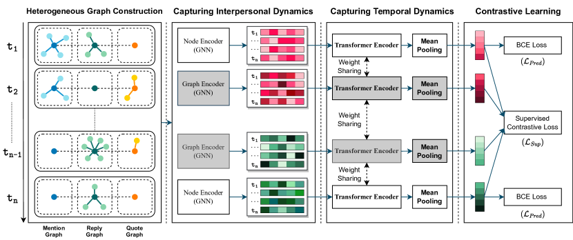
Figure 1. Architecture of ContrastEgo

3.2. ContrastEgo architecture.

ContrastEgo embraces four modules, (1) constructing users’ heterogeneous interactive graphs, (2) extracting the representations of users’ interaction snapshots using graph neural networks, (3) modeling the sequences of snapshots using attention mechanism, and (4) depression detection using contrastive learning. We first use a pre-trained RoBERTa model (Loureiro et al., 2022; Barbieri et al., 2020), trained on the Twitter corpus, to obtain the embeddings of all tweets posted by each user during each time period (snapshot). The averaged embedding obtained for each user is treated as the attributes of the corresponding node in each user’s ego-network. Next, for each user, we construct her heterogeneous interactive graph, where each snapshot in such dynamic graph contains the three distinct types of interactions between users and their friends (i.e., replies, mentions, and quote-tweets). In order to capture the interpersonal dynamics on social media to identify depression status for each snapshot, we utilize graph neural networks to encode social interactions and extract the latent user representations for each snapshot at multiple scales. In order to capture the temporal dynamics of depression, we utilize a transformer architecture to encode the sequences of snapshots using attention mechanism. At last, we adopt supervised contrastive learning to maximize the agreement of users’ representations extracted at different scales and minimize the agreement of users’ representations between the individuals with depression and those without depression. Given the contrastive loss $\mathcal{L}_{Con}$ and the binary cross-entropy loss $\mathcal{L}_{Pred}$, the loss function which ContrastEgo aims to optimize can be represented as follows:

(1) $$\mathcal{L}=\alpha\mathcal{L}_{Con}+\mathcal{L}_{Pred},$$

where $\alpha$ is a trade-off coefficient.

4. Methodologies

4.1. Heterogeneous interactive graphs

Feature engineering, a prevalent approach in prior literature (Chatterjee et al., 2021; Deshpande and Rao, 2017; Preoţiuc-Pietro et al., 2015; De Choudhury et al., 2021; Tadesse et al., 2019; Shen et al., 2017; Ghosh and Anwar, 2021), has been known to have many limitations. To capture the linguistic characteristics of users and their friends, ContrastEgo utilizes pre-trained NLP models such as BERT (Devlin et al., 2018), XLNet (Yang et al., 2019) and RoBERTa (Liu et al., 2019a) to extract the embeddings of all tweets posted by each user/friend during each time period (snapshot). The averaged embedding obtained for each user/friend is treated as the attributes of the corresponding node in each user’s ego-network.

For each user, we create her ego-network graph for each specific interaction type where each edge attribute value is set as the number of interactions in that type between the user and each of her friends. The embeddings obtained from the pretrained RoBERTa model are adopted as the node features. We then merge these three ego-network graphs for each user into a heterogeneous graph with each edge being a 3-dimensional vector representing the strengths of different interaction types (replies, mentions, or quote-tweets). Given a user’s information, we only keep those friends with whom she interacts. In other words, if a friend is missing all three interaction types with the associated user, that friend is pruned. By constructing a heterogeneous graph to model the interactions within the graph, we aim to better capture the complexity and richness of real-world social networks and gain insights into how social interactions can influence behavior.

In addition, we also propose a graph combination technique to enhance training efficiency. Instead of processing each time period one at a time, we combine all the graphs together for efficient computation. Let $G_{t}=(V_{t},E_{t})$ denote the snapshot of the graph at time step $t$, where $|V_{t}|$ represents the cardinality of nodes and $|E_{t}|$ represents the cardinality of edges. The aggregated graph $G^{\prime}=(V^{\prime},E^{\prime})$ is defined as the union of all graph snapshots from an individual, such that $V^{\prime}=\bigcup_{t=1}^{T}V_{t}$ and $E^{\prime}=\bigcup_{t=1}^{T}E_{t}$, where $T$ represents the total number of time periods. The resulting graph $G^{\prime}$ provides a global perspective of the ego nodes over time, where each graph snapshot is considered as a connected component. The properties of the resulting graph $G^{\prime}$ are: (1) $|V^{\prime}|=\sum_{t=1}^{T}|V_{t}|$, (2) $|E^{\prime}|=\sum_{t=1}^{T}|E_{t}|$, and (3) the number of connected components of $G^{\prime}$ equals $T$. This implies that the nodes in G’ represent the same entities at different points in time, but they are not directly connected to each other in the aggregate graph. This aggregated graph is then used for capturing interpersonal dynamics.

4.2. Capturing interpersonal dynamics

Recently, several studies have been proposed to extract multi-scale substructure features that are critical in understanding the underlying relationships in social networks using graph convolution (Zhang et al., 2019; Kipf and Welling, 2017). Let $G$ be an undirected graph of $n\in\mathbb{N}$ nodes and an adjacency matrix $\mathbf{A}\in\mathbb{Z}^{n\times n}$. An augmented adjacency matrix of $G$ is defined as $\mathbf{\tilde{A}}=\mathbf{A}+I_{n}$. For row-wise normalization, a diagonal degree matrix of $\mathbf{D}$ is defined as $\mathbf{\tilde{D}}_{i,i}=\sum_{j}\mathbf{\tilde{A}}_{i,j}$. A matrix of learnable parameters is defined as $\mathbf{W}\in\mathbb{R}^{c\times c^{\prime}},c^{\prime}\in\mathbb{N}$, where $c^{\prime}$ is the number of output feature channels. Suppose that the node feature matrix is $\mathbf{X}\in\mathbb{R}^{n\times c},c\in\mathbb{N}$ and a non-linear activation function is denoted by $\sigma$. The graph convolution operation can be defined as follows:

(2) $$\mathbf{Z}=\sigma\left(\tilde{\mathbf{D}}^{-1}\tilde{\mathbf{A}}\mathbf{X}\mathbf{W}\right),$$

where graph convolution aggregates information about the local substructure by smoothing information about nodes in the local neighborhood. To extract the multi-scale substructure features, multiple graph convolution layers are stacked, as follows:

(3) $$\mathbf{Z}^{(l+1)}=\sigma\left(\tilde{\mathbf{D}}^{-1}\tilde{\mathbf{A}}\mathbf{Z}^{(l)}\mathbf{W}^{(l)}\right),$$

where $\mathbf{Z}^{(0)}=X$ and $\mathbf{W}^{(l)}\in\mathbb{R}^{c_{l}\times c_{l+1}}$.

ContrastEgo adopts graph convolution to capture the interpersonal interactions within each snapshot in the created dynamic heterogeneous interactive graph. ContrastEgo updates the node embeddings represented by $H^{(l+1)}$ as follows:

(4) $$\begin{split}\mathbf{H}^{(l+1)}\leftarrow\sigma(\sum_{r\in R}(\tilde{\mathbf{A}_{r}}\mathbf{H}^{(l)}\mathbf{W}^{(l)}_{r})),\end{split}$$

where $\mathbf{H}^{(l)}$ refers to the node features when $l=0$, and the activation output of the $l^{th}$ layer for $l>0$, $\tilde{\mathbf{A}_{r}}$ is the normalized adjacency matrix for edge type $r$, $\mathbf{W}^{(l)}_{r}$ is the learnable weight matrix for layer $l$ with respect to edge type $r$, $R$ represents a set of edge types (mention, reply, and quote). The GELU activation function was used in our experiments.

4.3. Capturing temporal dynamics

Attention mechanism (Vaswani et al., 2017) has greatly improved the ability to capture dependencies among the elements of sequential input, especially in long sequences. ContrastEgo leverages a transformer encoder, which comprises multi-head self-attention networks and feed-forward neural networks to capture the temporal dynamics. The input sequences for the transformer encoder are created by rearranging the outputs of the heterogeneous graph learning module. The transformer encoder operates by computing three distinct representations of the input sequence. These representations, namely the query $Q=XW_{Q}$, key $K=XW_{K}$, and value $V=XW_{V}$ representations, are computed by applying linear transformations to the input sequence $X$, using learnable parameters $W_{Q}$, $W_{K}$, and $W_{V}$, respectively. Subsequently, attention scores for a sequence are computed as follows:

(5) $$Attention(Q,K,V)=softmax(\frac{QK^{T}}{\sqrt{d_{k}}})V$$

where $d_{k}$ is the dimension of $K$. The attention scores represent varying levels of importance to the ego nodes at different time periods, based on their relevance to the current query representation. The final output representation of the sequence is then derived by taking the dot-product of the attention scores and value representation. To ensure accurate evaluations of depression progression, we adopted positional encodings (Vaswani et al., 2017) into the transformer encoder. This enhances the model’s perception of the relative positions of ego nodes in the input sequence and enables it to understand temporal relationships between changes in a person’s social media behavior, such as post interactions and content. Proper consideration of the order of these behaviors is crucial in determining depression progression, as the arrangement can significantly impact the interpretation of a person’s mental state. For example, a decrease in depression symptoms followed by an increase may indicate worsening, while the reverse scenario may indicate improvement. The positional encodings, denoted by $\{p^{1},\dots,p^{t}\}\in\mathcal{R}^{d}$, are added element-wise to the input sequence $x^{i}$, where $i\in[1,t]$ and $t$ is the total number of time periods. Mathematically, the element-wise addition can be represented as $x^{i}+p^{i}$, where $x^{i}\in\mathcal{R}^{d}$ is the input embedding of the $i^{th}$ time period and $p^{i}\in\mathcal{R}^{d}$ is the positional embedding of the $i^{th}$ time period. After a fixed positional encoding vector $p^{i}\in\mathbb{R}^{d}$ is added to each input element of the sequence, the resulting sequence is then passed through the transformer encoder. To obtain a comprehensive user representation, we opt for a more simplistic approach by utilizing mean pooling on the encoded sequence rather than introducing a [CLS] token for classification.

(6) $$\begin{split}\mathcal{X}&\leftarrow Pooling(TransformerEncoder(\{x^{i}+p^{i}\})),i\in[1,t]\\ \end{split}$$

4.4. Supervised Contrastive Learning

ContrastEgo utilizes a supervised contrastive learning method to maximize the agreement of users’ representations extracted at different scales and minimize the agreement of users’ representations between the individuals with depression and those without depression. As shown in Figure 1, the node encoder and the graph encoder constitute the node- and graph-level views, respectively. Both views are then fed into the same transformer encoder, which learns to attend to temporal changes of the egos as well as the impact of users’ social circles. The transformer encoder’s output is then further processed by applying mean pooling over each sequence representation to obtain the overall node- and graph-level representations of the user for depression detection. The objective of supervised contrastive learning is to learn the representations of the data such that the representations of the positive pairs are closer to each other and the representations of the negative pairs are farther apart in the embedding space. Thus, we employ a projection neural network for contrastive learning to encourage the network to maximize agreement between positive pairs (same-group node-graph) and disagreement between negative pairs (different-group node-graph). This is predicated on the understanding that a person’s social milieu, including their relationships and social support, plays a role in the progression of depression (Pirayesh et al., 2021; Ivan et al., 2022; De Choudhury et al., 2021). A popular contrastive learning framework, SimCLR (Chen et al., 2020), only permits one positive sample to be paired with each anchor and considers all other augmented examples as negative examples. ContrastEgo adopts supervised contrastive loss (Khosla et al., 2020), which extends the self-supervised contrastive loss by taking into account class label information. The supervised contrastive loss is formulated as follows:

(7) $$\mathcal{L}_{sup}=\sum_{u\in U}\frac{-1}{|P(u)|}\sum_{p\in P(u)}\log\frac{e^{(z_{u}\cdot z_{p}/\tau)}}{\sum_{a\in A(u)}e^{(z_{u}\cdot z_{a}/\tau)}}$$

where $U$ is the set of all unique samples in the multiviewed batch, $P(u)$ is the set of indices of all positives in the multiviewed batch distinct from $u$, $z_{u}$ and $z_{p}$ are the embeddings of anchor and positive, respectively and $A(u)$ is the set of all negatives in the multiviewed batch distinct from $u$. Here, $\tau$ is a temperature hyperparameter.

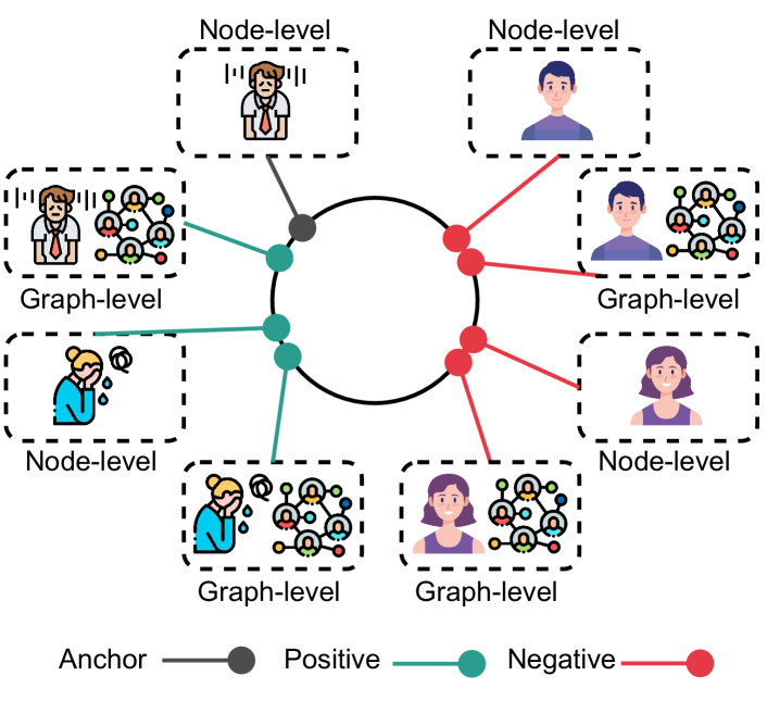
Figure 2. Illustration of Supervised Contrastive Learning

Figure 2 visually represents the concept of supervised contrastive learning in ContrastEgo. This approach utilizes both node-level and graph-level embeddings to enhance the learning process. To demonstrate this concept, we take the example of an individual with depression as the anchor. In supervised contrastive learning, individuals with depression (node-level view) and their social circles (graph-level view) are considered positive examples while the rest of the control group is regarded as negatives. This approach results in an embedding space where individuals belonging to the same class (depression) are grouped closer together, while individuals from different classes (control group) are separated further apart.

5. Experiment

In this section, we empirically show the superiority of ContrastEgo over the state-of-the-art methods.

5.1. Baselines

• GCN (Kipf and Welling, 2017). This method utilizes the Laplacian matrix of the graph to perform convolution operations on the node features.

• GraphSAGE (Hamilton et al., 2017). This method uses k-hop sampling to aggregate features from the sampled local neighborhood.

• GAT (Velickovic et al., 2018). This method employs self-attention mechanisms to weigh the importance of different nodes in the ego’s local network.

• MentalNet (Ivan et al., 2022). This method models three different types of interaction on social media (reply, mention, and quote), after which DGCNN (Zhang et al., 2018) is applied to generate the user representation as a graph. The LSTM autoencoder was replaced by a pretrained RoBERTa model (Loureiro et al., 2022; Barbieri et al., 2020) in our experiments for a fair comparison.

• DySAT (Sankar et al., 2020). This method leverages a GAT layer to obtain structural information and later employs self-attention mechanisms to capture temporal dependencies.

Table 1. Statistics of PsycheNet-G

	Users	Friends per user				Replies per user				Mentions per user				Quote-Tweets per friend
	Sum	Min	Max	Mean	Sum	Min	Max	Mean	Sum	Min	Max	Mean	Sum	Min	Max	Mean	Sum
Depressed group	$242$	$1$	$518$	$63$	$15,321$	$1$	$19,414$	$1,379$	$333,799$	$1$	$17,885$	$891$	$215,722$	$1$	$461$	$35$	$8,470$
Control group	$349$	$1$	$448$	$89$	$31,103$	$1$	$132,907$	$3,119$	$1,088,470$	$1$	$63,532$	$1,804$	$629,437$	$1$	$22,328$	$283$	$98,700$

5.2. Dataset

In our study, we utilized the PsycheNet-G dataset (Ivan et al., 2022), composed of 242 users diagnosed with depression and 349 individuals as the control group. Table 1 shows the statistics of the PsycheNet-G dataset. To generate user representations, each tweet was processed to create a tweet embedding utilizing the pre-trained RoBERTa model (Liu et al., 2019b), twitter-roberta-base-sep2022 (Loureiro et al., 2022; Barbieri et al., 2020), specifically trained on millions of tweets. In the case of dynamic/temporal neural networks, the node features of users and friends were represented by the mean of the corresponding tweet embeddings. On the other hand, for non-temporal neural networks, such as MentalNet, GCN, GAT, and GraphSAGE, the node features of users and friends were represented by the mean of the tweet embeddings throughout the user’s history, and the adjacent matrix was represented by the aggregation of the adjacent matrices of all time periods.

5.3. Research Questions

To evaluate the effectiveness of our proposed model, we evaluated our model based on three research questions:

• To what extent does the availability of user-generated content affect the accuracy of depression prediction in a scenario where access and usage of user data are limited?

• Is incorporating information from an individual’s social network an effective method for detecting depression?

• How does the duration of observation from social networks affect the prediction of depression onset and progression?

Based on these research questions, we processed the PsycheNet-G dataset by imposing different numbers of tweets, friends, and periods, as specified in Section 5.5. For different numbers of tweets per period and the number of friends per period, we applied uniform random sampling of tweets and friends, respectively. Any data in a period where the user had insufficient tweets or friends were not considered. For varying the length of every period, any data in a period where the user had insufficient tweets and friends were not considered. Figure 3 illustrates the distribution of data collection duration for all users. The y-axis represents the number of users whose data were collected for a certain duration.

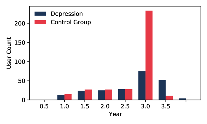
Figure 3. The Distribution of the PsycheNet-G dataset

5.4. Experiment Settings

In this study, we presented the performance of each method in terms of precision, recall, F₁, and AUC-ROC scores. All experiments were performed using Python v3.9, PyTorch v1.11.0 with an Intel(R) Core(TM) i7-7700HQ CPU (at 2.80GHz) and a GTX 1070Ti GPU (with 8 GB RAM). The model evaluation was performed using rigorous five-fold cross-validation evaluations, and the reported results were the average of ten runs. We obtained the implementation code for the baseline methods either from the PyTorch Geometric package or their official web pages. Unless otherwise specified, the default number of tweets per period is 5, the number of friends per period is 4, and the duration of each period is 12 months. To facilitate reproducibility, Table 2 presents the hyperparameter configuration employed in our experiments.

Table 2. Hyperparameter configuration

Parameter	Values
Learning Rate	1e-4
Batch Size	64
Number of GNN layers	3
Node Embedding Dimension	768
Output dimension of GNN	64
Final Embedding Dimension	64

Table 3. Performance comparison by varying the number of tweets in each time period

	1 tweet							3 tweet							5 tweet
	Healthy (0)				Depessed (1)			Healthy (0)				Depessed (1)			Healthy (0)				Depessed (1)
	P	R	F1	AUC	P	R	F1	P	R	F1	AUC	P	R	F1	P	R	F1	AUC	P	R	F1
GCN	0.83	0.82	0.82	0.76	0.69	0.70	0.69	0.85	0.85	0.85	0.80	0.74	0.74	0.74	0.87	0.88	0.87	0.82	0.79	0.77	0.78
GAT	0.84	0.83	0.83	0.77	0.72	0.71	0.71	0.85	0.85	0.85	0.79	0.74	0.73	0.73	0.88	0.85	0.86	0.82	0.76	0.80	0.78
GraphSAGE	0.82	0.86	0.84	0.77	0.73	0.67	0.70	0.85	0.86	0.85	0.79	0.75	0.73	0.73	0.86	0.88	0.87	0.82	0.79	0.76	0.77
DySAT	0.85	0.84	0.84	0.79	0.72	0.73	0.72	0.89	0.82	0.85	0.82	0.73	0.82	0.76	0.89	0.86	0.87	0.84	0.78	0.82	0.79
MentalNet	0.88	0.85	0.86	0.82	0.76	0.79	0.77	0.89	0.85	0.86	0.83	0.76	0.81	0.77	0.88	0.89	0.88	0.84	0.80	0.78	0.78
ContrastEgo	0.90	0.86	0.88	0.85	0.77	0.83	0.80	0.91	0.86	0.88	0.86	0.78	0.86	0.81	0.92	0.88	0.90	0.88	0.81	0.88	0.84

Table 4. Performance comparison by varying the number of friends in each time period

	2 friend							4 friend							8 friend
	Healthy (0)				Depessed (1)			Healthy (0)				Depessed (1)			Healthy (0)				Depessed (1)
	P	R	F1	AUC	P	R	F1	P	R	F1	AUC	P	R	F1	P	R	F1	AUC	P	R	F1
GCN	0.87	0.86	0.87	0.83	0.77	0.79	0.78	0.87	0.88	0.87	0.82	0.79	0.77	0.78	0.90	0.82	0.85	0.82	0.74	0.82	0.78
GAT	0.87	0.87	0.87	0.82	0.78	0.77	0.77	0.88	0.85	0.86	0.82	0.76	0.80	0.78	0.87	0.87	0.87	0.82	0.78	0.77	0.77
GraphSAGE	0.86	0.87	0.87	0.82	0.78	0.76	0.77	0.86	0.88	0.87	0.82	0.79	0.76	0.77	0.87	0.87	0.87	0.82	0.78	0.76	0.77
DySAT	0.89	0.85	0.86	0.83	0.77	0.82	0.79	0.89	0.86	0.87	0.84	0.78	0.82	0.79	0.89	0.84	0.87	0.84	0.76	0.83	0.79
MentalNet	0.88	0.88	0.87	0.83	0.79	0.79	0.78	0.88	0.89	0.88	0.84	0.80	0.78	0.78	0.89	0.89	0.89	0.85	0.82	0.80	0.81
ContrastEgo	0.90	0.87	0.88	0.85	0.79	0.83	0.81	0.92	0.88	0.90	0.88	0.81	0.88	0.84	0.92	0.90	0.91	0.88	0.84	0.86	0.85

Table 5. Performance comparison by varying the duration of time period

	3 months							6 months							12 months
	Healthy (0)				Depessed (1)			Healthy (0)				Depessed (1)			Healthy (0)				Depessed (1)
	P	R	F1	AUC	P	R	F1	P	R	F1	AUC	P	R	F1	P	R	F1	AUC	P	R	F1
GCN	0.89	0.89	0.89	0.85	0.81	0.80	0.81	0.88	0.84	0.86	0.82	0.73	0.80	0.76	0.87	0.88	0.87	0.82	0.78	0.76	0.77
GAT	0.90	0.87	0.88	0.85	0.79	0.82	0.81	0.88	0.85	0.86	0.82	0.74	0.79	0.77	0.88	0.85	0.87	0.82	0.75	0.80	0.77
GraphSAGE	0.89	0.88	0.89	0.85	0.80	0.82	0.81	0.88	0.86	0.87	0.83	0.76	0.79	0.77	0.86	0.88	0.87	0.82	0.79	0.75	0.77
DySAT	0.91	0.87	0.89	0.85	0.79	0.84	0.81	0.88	0.85	0.87	0.82	0.75	0.80	0.77	0.89	0.86	0.87	0.84	0.78	0.82	0.79
MentalNet	0.90	0.89	0.89	0.86	0.81	0.82	0.82	0.88	0.90	0.89	0.84	0.81	0.78	0.79	0.87	0.89	0.88	0.83	0.79	0.77	0.78
ContrastEgo	0.93	0.89	0.91	0.89	0.82	0.89	0.85	0.92	0.87	0.89	0.87	0.79	0.86	0.82	0.92	0.88	0.90	0.87	0.80	0.87	0.83

5.5. Evaluation

5.5.1. Impact of number of tweets (RQ₁)

In this study, we explored the impact of the number of tweets per user per period as it is a crucial parameter, that determines the quantity of data available for the model in the real world. We imposed a fixed number for each experiment, ranging from 1 to 5. The results, presented in Table 3, demonstrate that our proposed model ContrastEgo outperformed all baseline models when tested with varying levels of content resources. Also, when the quantity of data available to the model increased, the models’ performance also improved. This highlights the significance of using pretrained NLP models to obtain rich information from the tweets as node features, as well as the importance of having ample data from users to accurately detect depression. These results underscore the critical role that the number of tweets per user per period plays in depression detection and that utilizing more data leads to superior performance.

5.5.2. Impact of Number of Friends (RQ₂)

In this study, we aimed to comprehend the extent to which social connections contribute to the identification of depression by manipulating the number of friends per user per period from 2 to 8. The results, as displayed in Table 4, show that ContrastEgo significantly outperformed all the baselines by considering both the structural and temporal aspects of social interactions in depression detection. Additionally, the empirical results highlight the importance of considering social connections as a valuable source of information in depression detection and indicate the potential for enhanced performance through the integration of more information from an individual’s social milieu.

5.5.3. Impact of Interval of Period (RQ₃)

In order to gauge the effect of the temporal resolution on the performance of the models, we conducted a comprehensive evaluation by varying the duration of the observational intervals from 3 to 12 months. This experimental setting aimed to examine the relationship between the frequency of observations and the ability of the models to detect depression. The results, as presented in Table 5, indicate a clear correlation between the reduction in the interval duration and an improvement in the models’ performance. This can be attributed to the fact that shorter intervals provide more recent and frequent observations of the individual’s linguistic and social patterns, thereby increasing the sensitivity of the model to detect depression. Furthermore, the results demonstrate that ContrastEgo is robust in early detection of depression even with longer observational intervals. This can be especially valuable in scenarios where a higher frequency of data collection is challenging.

5.6. Ablation Study

In this subsection, we conducted a series of ablation experiments to verify the effectiveness of each component used in ContrastEgo. The variants of ContrastEgo we compare are as follows:

• ContrastEgo. This is the complete version of our proposed model, including heterogeneous graph learning, temporal graph learning, supervised contrastive learning, and graph combination.

• ContrastEgo-C. This is a degraded version with the supervised contrastive learning component removed.

• ContrastEgo-HO. This is the degraded version with the heterogeneous graph learning replaced by homogeneous graph learning.

• ContrastEgo-H. In this degraded version, the heterogeneous graph learning module is removed.

• ContrastEgo-T. This is the degraded version with the transformer encoder module removed.

Table 6. num_friend: 4, period_in_months: 12

	1 tweet							3 tweet							5 tweet
	Healthy (0)				Depessed (1)			Healthy (0)				Depessed (1)			Healthy (0)				Depessed (1)
	P	R	F1	AUC	P	R	F1	P	R	F1	AUC	P	R	F1	P	R	F1	AUC	P	R	F1
ContrastEgo	0.90	0.86	0.88	0.84	0.77	0.83	0.80	0.91	0.86	0.88	0.86	0.77	0.85	0.81	0.92	0.88	0.90	0.87	0.80	0.87	0.83
ContrastEgo-C	0.90	0.84	0.87	0.83	0.74	0.83	0.78	0.90	0.83	0.87	0.84	0.74	0.84	0.79	0.91	0.86	0.88	0.85	0.78	0.84	0.81
ContrastEgo-H	0.84	0.76	0.80	0.75	0.63	0.74	0.68	0.85	0.81	0.83	0.78	0.69	0.74	0.71	0.87	0.82	0.85	0.80	0.72	0.78	0.75
ContrastEgo-T	0.89	0.86	0.88	0.84	0.77	0.81	0.79	0.90	0.85	0.88	0.84	0.76	0.84	0.80	0.89	0.87	0.88	0.85	0.79	0.82	0.80
ContrastEgo-HO	0.87	0.86	0.87	0.82	0.76	0.78	0.77	0.88	0.85	0.87	0.82	0.75	0.80	0.77	0.90	0.85	0.87	0.84	0.76	0.82	0.79

Table 7. num_tweet_per_period: 5, period_in_months: 12

	2 friend							4 friend							8 friend
	Healthy (0)				Depessed (1)			Healthy (0)				Depessed (1)			Healthy (0)				Depessed (1)
	P	R	F1	AUC	P	R	F1	P	R	F1	AUC	P	R	F1	P	R	F1	AUC	P	R	F1
ContrastEgo	0.90	0.87	0.89	0.85	0.79	0.82	0.81	0.92	0.88	0.90	0.87	0.80	0.87	0.83	0.92	0.90	0.91	0.88	0.83	0.85	0.84
ContrastEgo-C	0.89	0.87	0.88	0.84	0.78	0.80	0.79	0.91	0.86	0.88	0.85	0.78	0.84	0.81	0.91	0.88	0.90	0.86	0.80	0.85	0.82
ContrastEgo-H	0.88	0.80	0.84	0.80	0.70	0.80	0.75	0.87	0.82	0.85	0.80	0.72	0.78	0.75	0.88	0.83	0.86	0.82	0.73	0.80	0.76
ContrastEgo-T	0.87	0.91	0.89	0.84	0.83	0.76	0.79	0.89	0.87	0.88	0.85	0.79	0.82	0.80	0.90	0.91	0.90	0.86	0.84	0.82	0.83
ContrastEgo-HO	0.89	0.86	0.87	0.83	0.77	0.80	0.79	0.90	0.85	0.87	0.84	0.76	0.82	0.79	0.90	0.88	0.89	0.85	0.79	0.82	0.81

Table 8. num_tweet_per_period: 5, num_friend: 4

	3 months							6 months							12 months
	Healthy (0)				Depessed (1)			Healthy (0)				Depessed (1)			Healthy (0)				Depessed (1)
	P	R	F1	AUC	P	R	F1	P	R	F1	AUC	P	R	F1	P	R	F1	AUC	P	R	F1
ContrastEgo	0.93	0.89	0.91	0.89	0.82	0.89	0.85	0.92	0.87	0.89	0.87	0.79	0.86	0.82	0.92	0.88	0.90	0.87	0.80	0.87	0.83
ContrastEgo-C	0.92	0.89	0.90	0.87	0.81	0.86	0.83	0.91	0.88	0.89	0.86	0.79	0.84	0.82	0.91	0.86	0.88	0.85	0.78	0.84	0.81
ContrastEgo-H	0.90	0.88	0.89	0.85	0.80	0.82	0.81	0.88	0.87	0.88	0.83	0.77	0.78	0.78	0.87	0.82	0.85	0.80	0.72	0.78	0.75
ContrastEgo-T	0.92	0.92	0.92	0.89	0.86	0.87	0.86	0.90	0.89	0.89	0.85	0.80	0.82	0.81	0.89	0.87	0.88	0.85	0.79	0.82	0.80
ContrarstEgo-HO	0.92	0.89	0.91	0.88	0.82	0.87	0.84	0.91	0.86	0.88	0.85	0.77	0.84	0.80	0.90	0.85	0.87	0.84	0.76	0.82	0.79

5.6.1. Heterogeneous Graph Learning

This experiment investigated the effect of removing the heterogeneous graph learning component from ContrastEgo, denoted by ContrastEgo-H. This variant relied on the transformer encoder for depression prediction and disregarded information from social networks. Our results, shown in Table 6, Table 7, and Table 8, demonstrate a significant degradation in performance in all settings without heterogeneous graph learning. This highlights the critical significance of social network information in depression prediction, underscoring the importance of social networks as indicators of an individual’s behavior and emotional state. Furthermore, we compared the performance of ContrastEgo, to a version using homogeneous graph learning instead, denoted by ContrastEgo-HO. The results demonstrate that ContrastEgo outperformed ContrastEgo-HO, confirming that capturing heterogeneity within social networks is essential for accurate depression prediction. These results suggest that heterogeneous graph learning plays a crucial role in effectively capturing the structure of the social network, thereby improving performance.

5.6.2. Temporal Graph Learning

This experiment evaluated the impact of removing the transformer encoder component in regard to capturing temporal dependencies, denoted by ContrastEgo-T. Our results, displayed in Table 6, Table 7, and Table 8, exhibit that the model’s performance was slightly degraded without the transformer encoder component in most settings. This suggests that the temporal aspect of the user data is crucial in determining its contribution to the development of depression, as it may vary. Furthermore, the sequence of behaviors can have utterly distinct interpretations and influence on the development of depression, and, hence, should be considered accordingly.

5.6.3. Supervised Contrastive Learning

This experiment evaluated the impact of removing the supervised contrastive learning component, denoted by ContrastEgo-C, on the model’s performance. The results shown in Table 6, Table 7, and Table 8, exhibit that the model’s performance was slightly degraded without contrastive learning. This suggests that using contrastive learning effectively enhanced the representation of individuals with depression and contributes to the overall performance of the model. The results are further visualized through Figure 4, which serves to illustrate the differences between representation of individuals with and without depression in the embedding space.

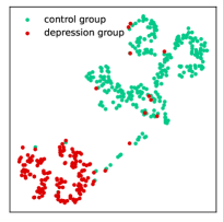
(a) ContrastEgo

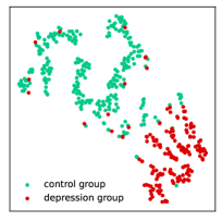
(b) ContrastEgo-C

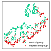
(c) ContrastEgo-H

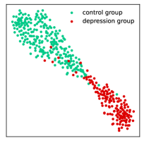
(d) ContrastEgo-T

Figure 4. t-SNE Visualization of User Representations

5.6.4. Graph Combination

The study compared the efficiency of the proposed graph combination technique to a variant without the graph combination component, denoted by ContrastEgo-GC. The processing time of ContrastEgo was significantly faster with an average of 2.15 seconds per epoch compared to the average of 19.92 seconds per epoch for ContrastEgo-GC. This is because the proposed technique processes multiple graph snapshots from the same user and graphs from different users together to achieve highly parallelizable processing.

6. Related Work

The utilization of online social media as a source of information for the study of mental health, specifically in the realm of depression detection, has been the subject of considerable scholarly attention in recent years. In particular, NLP techniques and feature engineering on social media data have been the focus of a plethora of studies aimed at detecting depression in an early stage.

Machine Learning-Based Depression Detection. Traditional machine learning-based approaches for depression detection focus on identifying relevant features from data and using them as input to machine learning models. Different feature extraction methods have been utilized, such as term-document matrix (TDM) and term frequency-inverse document frequency (TF-IDF) (Chatterjee et al., 2021), a bag-of-words model  (Deshpande and Rao, 2017), and linguistic inquiry and word count (LIWC) for categorizing words based on linguistic properties  (Preoţiuc-Pietro et al., 2015; De Choudhury et al., 2021). Several studies have explored the use of multiple feature engineering techniques. Tadesse  et al. (Tadesse et al., 2019) combined LIWC, Latent Dirichlet Allocation (LDA), and n-grams for feature extraction and evaluated with different classifiers. Shen et al. (Shen et al., 2017) extracted several depression-related features using LIWC, and LDA, and applied multimodal dictionary learning for sparse user representations.

Deep-Learning-Based Depression Detection. Deep learning methods have been increasingly used in recent years for the prediction of depression from social media data. For instance, Ghosh et al. (Ghosh and Anwar, 2021) employed an LSTM network based on a comprehensive set of user features and depression-related n-grams. Shah et al. (Shah et al., 2020) applied a bidirectional LSTM with various word embedding techniques. Yates (Yates et al., 2017) applied a CNN to each post, all of which are later merged with another convolutional layer to generate a user representation for prediction. Zogan et al. (Zogan et al., 2021) presented a model that integrates a CNN with a stacked bidirectional GRU (BiGRU) with Attention, drawing upon a fusion of user behavior and posting history features, where extraneous content is disregarded, to extract various features through LDA such as social network, emotions, depression domain-specific and topic features. Orabi  et al. (Husseini Orabi et al., 2018) explored the performance of various CNN and RNN models using a combination of word embedding techniques for embedding refinement. (Figuerêdo et al., 2022) combined a pre-trained NLP model with CNNs using both early and late fusion approaches. Ophir et al. (Ophir et al., 2020) predicted suicide risk from Facebook posts by considering multiple mediating factors, employing a hierarchical subnetwork architecture with a shared layer of fully connected nodes to mitigate the risk of overfitting. Pirayesh et al. (Pirayesh et al., 2021) proposed a method for obtaining user embeddings based on aggregated social media posts using a triplet network, after which dynamic mean shift pruning is used to identify homogeneous friends from social circles for prediction along with the target user. Mihov et al. (Ivan et al., 2022) constructed a heterogeneous graph capturing various types of interactions between users and friends with a sort pooling layer for graph classification.

Temporal/Dynamic Graph Learning. Temporal graph and dynamic graph learning are emerging fields that study the evolution and changes of graphs over time, and how to model these changes to capture the dynamic nature of real-world events. Pareja et al. (Pareja et al., 2020) introduces an RNN that incorporates the GCN weights and node embeddings to capture the temporal dynamics of graph data. Sankar et al. (Sankar et al., 2020) presented an approach that leverages the use of structural and temporal self-attention mechanisms for learning node representations over time. This method involves processing each graph snapshot through a structural self-attention network, adding positional embeddings, and finally learning the node representations through the temporal self-attention mechanism.

7. Conclusion

In conclusion, current depression detection methods have several limitations, particularly their dependence on feature engineering and inadequate consideration of time-varying factors. To tackle these limitations, we have proposed an early depression detection framework, ContrastEgo. Our framework effectively learns multi-scale user latent representations by capturing the topological dynamics of users’ social interactions through supervised contrastive learning. Our experiments on Twitter data reveal the importance of taking into account the influence of social circles and time-varying patterns in depression detection. The results demonstrate the superiority of ContrastEgo over existing state-of-the-art GNN-based methods. With up to 5% improvement in F1 score and 4% improvement in AUROC compared to the baseline methods, our framework provides a promising solution for early detection of depression.

References

- (1)
- who ([n. d.]) [n. d.]. Mental health in the Workplace. https://www.who.int/health-topics/mental-health
- Barbieri et al. (2020) Francesco Barbieri, Jose Camacho-Collados, Luis Espinosa Anke, and Leonardo Neves. 2020. TweetEval: Unified Benchmark and Comparative Evaluation for Tweet Classification. In Findings of the Association for Computational Linguistics: EMNLP 2020. Association for Computational Linguistics, Online, 1644–1650. https://doi.org/10.18653/v1/2020.findings-emnlp.148
- Chatterjee et al. (2021) Rinki Chatterjee, Rajeev Kumar Gupta, and Bhavana Gupta. 2021. Depression Detection from Social Media Posts Using Multinomial Naive Theorem. IOP Conference Series: Materials Science and Engineering 1022, 1 (jan 2021), 012095. https://doi.org/10.1088/1757-899X/1022/1/012095
- Chen et al. (2020) Ting Chen, Simon Kornblith, Mohammad Norouzi, and Geoffrey E. Hinton. 2020. A Simple Framework for Contrastive Learning of Visual Representations. In ICML (Proceedings of Machine Learning Research, Vol. 119). PMLR, 1597–1607.
- De Choudhury et al. (2021) Munmun De Choudhury, Michael Gamon, Scott Counts, and Eric Horvitz. 2021. Predicting Depression via Social Media. Proceedings of the International AAAI Conference on Web and Social Media 7, 1 (Aug. 2021), 128–137. https://doi.org/10.1609/icwsm.v7i1.14432
- Deshpande and Rao (2017) Mandar Deshpande and Vignesh Rao. 2017. Depression detection using emotion artificial intelligence. In 2017 International Conference on Intelligent Sustainable Systems (ICISS). 858–862. https://doi.org/10.1109/ISS1.2017.8389299
- Devlin et al. (2018) Jacob Devlin, Ming-Wei Chang, Kenton Lee, and Kristina Toutanova. 2018. Bert: Pre-training of deep bidirectional transformers for language understanding. arXiv preprint (2018).
- Figuerêdo et al. (2022) José Solenir L. Figuerêdo, Ana Lúcia L.M. Maia, and Rodrigo Tripodi Calumby. 2022. Early depression detection in social media based on deep learning and underlying emotions. Online Social Networks and Media 31 (2022), 100225. https://doi.org/10.1016/j.osnem.2022.100225
- Ghosh and Anwar (2021) Shreya Ghosh and Tarique Anwar. 2021. Depression Intensity Estimation via Social Media: A Deep Learning Approach. IEEE Transactions on Computational Social Systems 8, 6 (2021), 1465–1474. https://doi.org/10.1109/TCSS.2021.3084154
- Hamilton et al. (2017) William L. Hamilton, Rex Ying, and Jure Leskovec. 2017. Inductive Representation Learning on Large Graphs. In Proceedings of the 31st International Conference on Neural Information Processing Systems (NIPS’17). Curran Associates Inc., Red Hook, NY, USA, 1025–1035.
- Husseini Orabi et al. (2018) Ahmed Husseini Orabi, Prasadith Buddhitha, Mahmoud Husseini Orabi, and Diana Inkpen. 2018. Deep Learning for Depression Detection of Twitter Users. In Proceedings of the Fifth Workshop on Computational Linguistics and Clinical Psychology: From Keyboard to Clinic. Association for Computational Linguistics, New Orleans, LA, 88–97. https://doi.org/10.18653/v1/W18-0609
- Ivan et al. (2022) Mihov Ivan, Chen Haiquan, Qin Xiao, Ku Wei-Shinn, Yan Da, and Liu Yuhong. 2022. MentalNet: Heterogeneous Graph Representation for Early Depression Detection. In Proceedings of the 22nd IEEE International Conference on Data Mining.
- Jiang et al. (2018) H. Jiang, B. Hu, Z. Liu, G. Wang, L. Zhang, X. Li, and H. Kang. 2018. Detecting Depression Using an Ensemble Logistic Regression Model Based on Multiple Speech Features. Comput Math Methods Med 2018 (2018), 6508319.
- Khosla et al. (2020) Prannay Khosla, Piotr Teterwak, Chen Wang, Aaron Sarna, Yonglong Tian, Phillip Isola, Aaron Maschinot, Ce Liu, and Dilip Krishnan. 2020. Supervised Contrastive Learning. In Advances in Neural Information Processing Systems, H. Larochelle, M. Ranzato, R. Hadsell, M.F. Balcan, and H. Lin (Eds.), Vol. 33. Curran Associates, Inc., 18661–18673. https://proceedings.neurips.cc/paper/2020/file/d89a66c7c80a29b1bdbab0f2a1a94af8-Paper.pdf
- Kipf and Welling (2017) Thomas N. Kipf and Max Welling. 2017. Semi-Supervised Classification with Graph Convolutional Networks. In 5th International Conference on Learning Representations, ICLR 2017, Toulon, France, April 24-26, 2017, Conference Track Proceedings. OpenReview.net. https://openreview.net/forum?id=SJU4ayYgl
- Liu et al. (2019a) Yinhan Liu, Myle Ott, Naman Goyal, Jingfei Du, Mandar Joshi, Danqi Chen, Omer Levy, Mike Lewis, Luke Zettlemoyer, and Veselin Stoyanov. 2019a. Roberta: A robustly optimized bert pretraining approach. arXiv preprint (2019).
- Liu et al. (2019b) Yinhan Liu, Myle Ott, Naman Goyal, Jingfei Du, Mandar Joshi, Danqi Chen, Omer Levy, Mike Lewis, Luke Zettlemoyer, and Veselin Stoyanov. 2019b. RoBERTa: A Robustly Optimized BERT Pretraining Approach. https://doi.org/10.48550/ARXIV.1907.11692
- Loureiro et al. (2022) Daniel Loureiro, Francesco Barbieri, Leonardo Neves, Luis Espinosa Anke, and Jose Camacho-collados. 2022. TimeLMs: Diachronic Language Models from Twitter. In Proceedings of the 60th Annual Meeting of the Association for Computational Linguistics: System Demonstrations. Association for Computational Linguistics, 251–260. https://doi.org/10.18653/v1/2022.acl-demo.25
- Ophir et al. (2020) Yaakov Ophir, Refael Tikochinski, Christa S. C. Asterhan, Itay Sisso, and Roi Reichart. 2020. Deep neural networks detect suicide risk from textual facebook posts. Scientific Reports 10, 1 (07 Oct 2020), 16685. https://doi.org/10.1038/s41598-020-73917-0
- Pareja et al. (2020) Aldo Pareja, Giacomo Domeniconi, Jie Chen, Tengfei Ma, Toyotaro Suzumura, Hiroki Kanezashi, Tim Kaler, Tao Schardl, and Charles Leiserson. 2020. EvolveGCN: Evolving Graph Convolutional Networks for Dynamic Graphs. Proceedings of the AAAI Conference on Artificial Intelligence 34, 04 (Apr. 2020), 5363–5370. https://doi.org/10.1609/aaai.v34i04.5984
- Pirayesh et al. (2021) Jahandad Pirayesh, Haiquan Chen, Xiao Qin, Wei-Shinn Ku, and Da Yan. 2021. MentalSpot: Effective Early Screening for Depression Based on Social Contagion. In Proceedings of the 30th ACM International Conference on Information & Knowledge Management (CIKM ’21). Association for Computing Machinery, 1437–1446. https://doi.org/10.1145/3459637.3482366
- Preoţiuc-Pietro et al. (2015) Daniel Preoţiuc-Pietro, Johannes Eichstaedt, Gregory Park, Maarten Sap, Laura Smith, Victoria Tobolsky, H. Andrew Schwartz, and Lyle Ungar. 2015. The role of personality, age, and gender in tweeting about mental illness. In Proceedings of the 2nd Workshop on Computational Linguistics and Clinical Psychology: From Linguistic Signal to Clinical Reality. Association for Computational Linguistics, 21–30. https://doi.org/10.3115/v1/W15-1203
- S and Antony (2022) Adarsh S and Betina Antony. 2022. SSN@LT-EDI-ACL2022: Transfer Learning using BERT for Detecting Signs of Depression from Social Media Texts. In Proceedings of the Second Workshop on Language Technology for Equality, Diversity and Inclusion. Association for Computational Linguistics, 326–330. https://doi.org/10.18653/v1/2022.ltedi-1.50
- Sankar et al. (2020) Aravind Sankar, Yanhong Wu, Liang Gou, Wei Zhang, and Hao Yang. 2020. DySAT: Deep Neural Representation Learning on Dynamic Graphs via Self-Attention Networks. In Proceedings of the 13th International Conference on Web Search and Data Mining (WSDM ’20). 519–527. https://doi.org/10.1145/3336191.3371845
- Shah et al. (2020) Faisal Muhammad Shah, Farzad Ahmed, Sajib Kumar Saha Joy, Sifat Ahmed, Samir Sadek, Rimon Shil, and Md. Hasanul Kabir. 2020. Early Depression Detection from Social Network Using Deep Learning Techniques. In 2020 IEEE Region 10 Symposium (TENSYMP). 823–826. https://doi.org/10.1109/TENSYMP50017.2020.9231008
- Shen et al. (2017) Guangyao Shen, Jia Jia, Liqiang Nie, Fuli Feng, Cunjun Zhang, Tianrui Hu, Tat-Seng Chua, and Wenwu Zhu. 2017. Depression Detection via Harvesting Social Media: A Multimodal Dictionary Learning Solution. In Proceedings of the Twenty-Sixth International Joint Conference on Artificial Intelligence, IJCAI-17. 3838–3844. https://doi.org/10.24963/ijcai.2017/536
- Tadesse et al. (2019) Michael M. Tadesse, Hongfei Lin, Bo Xu, and Liang Yang. 2019. Detection of Depression-Related Posts in Reddit Social Media Forum. IEEE Access 7 (2019), 44883–44893. https://doi.org/10.1109/ACCESS.2019.2909180
- Vaswani et al. (2017) Ashish Vaswani, Noam Shazeer, Niki Parmar, Jakob Uszkoreit, Llion Jones, Aidan N Gomez, Ł ukasz Kaiser, and Illia Polosukhin. 2017. Attention is All you Need. In Advances in Neural Information Processing Systems, Vol. 30.
- Velickovic et al. (2018) Petar Velickovic, Guillem Cucurull, Arantxa Casanova, Adriana Romero, Pietro Liò, and Yoshua Bengio. 2018. Graph Attention Networks. In 6th International Conference on Learning Representations, ICLR 2018, Vancouver, BC, Canada, April 30 - May 3, 2018, Conference Track Proceedings. OpenReview.net. https://openreview.net/forum?id=rJXMpikCZ
- Yang et al. (2019) Zhilin Yang, Zihang Dai, Yiming Yang, Jaime Carbonell, Russ R Salakhutdinov, and Quoc V Le. 2019. Xlnet: Generalized autoregressive pretraining for language understanding. NeurIPS (2019).
- Yates et al. (2017) Andrew Yates, Arman Cohan, and Nazli Goharian. 2017. Depression and Self-Harm Risk Assessment in Online Forums. In Proceedings of the 2017 Conference on Empirical Methods in Natural Language Processing. Association for Computational Linguistics, Copenhagen, Denmark, 2968–2978. https://doi.org/10.18653/v1/D17-1322
- Zhang et al. (2018) Muhan Zhang, Zhicheng Cui, Marion Neumann, and Yixin Chen. 2018. An End-to-End Deep Learning Architecture for Graph Classification. Proceedings of the AAAI Conference on Artificial Intelligence 32, 1 (Apr. 2018). https://doi.org/10.1609/aaai.v32i1.11782
- Zhang et al. (2019) Si Zhang, Hanghang Tong, Jiejun Xu, and Ross Maciejewski. 2019. Graph convolutional networks: a comprehensive review. (2019).
- Zogan et al. (2021) Hamad Zogan, Imran Razzak, Shoaib Jameel, and Guandong Xu. 2021. DepressionNet: Learning Multi-Modalities with User Post Summarization for Depression Detection on Social Media. In Proceedings of the 44th International ACM SIGIR Conference on Research and Development in Information Retrieval (SIGIR ’21). Association for Computing Machinery, 133–142. https://doi.org/10.1145/3404835.3462938