Efficient Beamforming Designs for IRS-Aided DFRC Systems

Abstract

This short tutorial presents several ideas for designing dual function radar communication (DFRC) systems aided by intelligent reflecting surfaces (IRS). These problems are highly nonlinear in the IRS parameter matrix, and further, the IRS parameters are subject to non-convex unit modulus constraints. We present classical semidefinite relaxation based methods, low-complexity minorization based optimization methods, low-complexity Riemannian manifold optimization methods, and near optimal branch and bound based methods.

I INTRODUCTION

The wireless spectrum becomes increasingly congested and spectrum reuse is necessary to achieve high spectral efficiency. How to share the spectrum between radar and communication systems, has attracted significant attention for decades [1]. Recently, dual function radar communication (DFRC) systems [2, 3, 4] provide a new paradigm for spectrum sharing. DFRC systems reuse the transmit waveform and share a common hardware platform between the radar and communication functionalities. As a result, DFRC systems achieve high spectral efficiency and reduced hardware cost.

In order to have access to higher bandwidth, which is needed for higher sensing resolution and higher communication rates, future wireless networks will need to use high frequencies. However, such frequencies experience high attenuation. Intelligent reflecting surface (IRS) have the potential to create a smart propagation environment, and combat the effects of attenuation. An IRS is a passive array composed of elements of printed dipoles, each of which can change the phase of the impinging electromagnetic wave in a computer controlled fashion [5, 6]. These elements can cooperatively beamform towards desired directions, or avoid undesired directions. When used with a DFRC system, an IRS platform can create extra paths between the DFRC radar the communication users and the radar targets. Thereby, IRS can assist the sensing and communication functions of the DFRC system simultaneously, by customizing the wireless propagation environment for the radar targets [7] and communication users [5].

The design of IRS-assisted DFRC systems is a challenging non-convex problem. The radar precoder and the IRS parameters are coupled variables, and need to be jointly designed. In addition, the design problem consists of non-convex objectives, non-convex manifold constraints, and high order functions in the objective or constraints [8, 9, 10, 11].

In this paper we present different methods for addressing the challenging design of IRS-aided DFRC systems. We start with classical semidefinite relaxation (SDR) based optimization methods. Then, we present two closed-form expression based algorithms, which are applicable to large IRS scenarios, where the design complexity is high. One of them is based on minorization or MM [12], and the other one is based on Riemannian manifold optimization [9]. We should note that large size IRS are needed in order to achieve high beamforming gain [13]. Finally, we present benchmark near-optimal branch-and-bound based algorithm to enhance the system performance by iteratively selecting the current best solution from local optima.

II SYSTEM MODEL

Figure 1: IRS-assisted DFRC system.

Let us consider the IRS-assisted DFRC system shown Fig. 1. The collocated DFRC transmitter and receiver are respectively modeled as $N_{T}$- and $N_{R}$-element uniform linear arrays (ULAs). For both the inter-element space is $d$. The radar transmits a single waveform, which is designed to track a non-line-of-sight (NLOS) point target, while simultaneously conveying information to a single-antenna communication user. The system is assisted by an $N$-element IRS. Perfectly known flat fading channels are assumed. The signal emitted from the DFRC radar is

$$\mathbf{x}=\mathbf{w}s,$$ (1)

where $\mathbf{w}\in\mathbb{C}^{N_{T}\times 1}$ is the radar precoding vector, and $s$ is the radar probing waveform that also contains communication information. $s$ is assumed to be zero-mean while with unit variance. Since there is no direct path to the target, the transmitted signal reaches the target after being reflected by the IRS, then it is reflected by the target, and arrives at the radar receiver after being reflected by the IRS again. The signal at the radar receiver can be expressed as

$$\mathbf{y}_{R} = {\beta\mathbf{H}_{ul}\mathbf{\Phi}\mathbf{a}_{I}(\psi_{a},\psi_{e})\mathbf{a}_{I}^{T}(\psi_{a},\psi_{e})\mathbf{\Phi}\mathbf{H}_{dl}}\mathbf{x}+\mathbf{n}_{R}$$ (2)

$$= \mathbf{C}_{T}\mathbf{x}+\mathbf{n}_{R},$$

where $\beta$ is the channel corresponding to the radar-IRS-target-IRS-radar path; $\mathbf{H}_{ul}$ and $\mathbf{H}_{dl}$ are respectively the normalized IRS-radar and radar-IRS channels; $\mathbf{\Phi}=\text{diag}([e^{j\phi_{1}},\cdots,e^{j\phi_{n}},\cdots,e^{j\phi_{N}}])$ is a diagonal matrix denoting the IRS parameter, with $\phi_{n}\in[0,2\pi)$ denoting the phase shift induced by the $n$-th IRS element; $\mathbf{a}_{I}(\psi_{a},\psi_{e})$ is the IRS steering vector, where $\psi_{a}$ and $\psi_{e}$ are respectively the target angles relative to the IRS in the azimuth and elevation planes; $\mathbf{n}_{R}\sim\mathcal{CN}(\mathbf{0}_{N_{R}\times 1},\sigma_{R}^{2}\mathbf{I}_{N_{R}})$ is the additive white Gaussian noise (AWGN) at the radar receiver, where $\sigma_{R}^{2}$ is the noise power at each radar receive antenna.

The received signal at the communication user is

$$y_{U}=(\beta_{H}^{\frac{1}{2}}\mathbf{f}^{T}\mathbf{\Phi}\mathbf{H}_{dl}+\mathbf{g}^{T})\mathbf{w}s+n_{U}=\mathbf{c}_{U}^{T}\mathbf{w}s+n_{U},$$ (3)

where $\beta_{H}$ is the path-loss of the radar-IRS channel, $\mathbf{f}\in\mathbb{C}^{N\times 1}$ is the user-IRS channel, $\mathbf{g}\in\mathbb{C}^{N_{T}\times 1}$ is the user-radar channel, and $n_{U}\sim\mathcal{CN}(0,\sigma_{U}^{2})$ is AWGN at the user.

The SNR at radar receiver and communication user are

$$\!\!\!\!\!\!\!\!\!\!\!\!\!\!\!\gamma_{R}=(1/{\sigma_{R}^{2}})\mathrm{tr}\!\left[{\mathbf{C}_{T}\mathbf{w}\mathbf{w}^{H}\mathbf{C}_{T}^{H}}\right],$$ (4)

$$\!\!\!\!\!\!\!\!\!\!\!\!\!\!\!\gamma_{U}=(1/{\sigma_{U}^{2}})|\mathbf{c}_{U}^{T}\mathbf{w}|^{2}.$$ (5)

III SYSTEM DESIGN

Let us design the radar precoder $\mathbf{w}$ and IRS parameter $\mathbf{\Phi}$ so that we maximize the weighted sum of the SNRs at the radar receiver and user, while meeting certain constraints, i.e.,

$$\max_{\mathbf{w},\mathbf{\Phi}} \;\;\;\;\alpha\gamma_{R}+(1-\alpha)\gamma_{U}$$ (6a)

$$\mathrm{s.t.} \;\;\;\;\mathrm{tr}\!\left[{\mathbf{w}\mathbf{w}^{H}}\right]=P_{R}$$ (6d)

$$\;\;\;\;\|\mathbf{w}\mathbf{w}^{H}-\mathbf{R}_{D}\|_{F}^{2}\leq\gamma_{BP}$$

$$\;\;\;\;|\mathbf{\Phi}_{n,n}|=1,\;\;\forall n=1,\cdots,N$$

where the real constant $\alpha$ is a weight factor; (6d) ensures that the power of the transmitted waveform stays within the power budget, $P_{R}$; (6d) ensures that the maximum beampattern deviation from a desired one is less than a threshold $\gamma_{BP}$, with $\mathbf{R}_{D}$ denoting the covariance matrix of the transmitted waveform; (6d) implies that each element of $\mathbf{\Phi}$ has unit modulus. The latter constraint models the fact that the IRS does not have any radio frequency (RF) chains and thus cannot change the magnitude of the reflected signal. Therefore, it only changes the phase of the impinging signal.

Problem (6) is highly non-convex due to the following facts. (i) The variables $\mathbf{w}$ and $\mathbf{\Phi}$ are coupled with each other. (ii) The radar SNR, $\gamma_{R}$, is fourth order in $\mathbf{\Phi}$, since $\gamma_{R}$ is quadratic into $\mathbf{C}_{T}$ per Eq. (4), where $\mathbf{C}_{T}$ is quadratic in $\mathbf{\Phi}$ per Eq. (2). (iii) (6d) is non-convex unit modulus constraint (UMC) on $\mathbf{\Phi}$.

To decouple $\mathbf{w}$ and $\mathbf{\Phi}$, we can separate (6) into to two sub-problems, i.e., optimize with respect to $\mathbf{w}$ by fixing $\mathbf{\Phi}$, and optimize with respect to $\mathbf{\Phi}$ by fixing $\mathbf{w}$. The two sub-problems are solved alternatingly till convergence is reached [14].

III-A First sub-problem: Solve for $\mathbf{w}$ with fixed $\mathbf{\Phi}$

The first sub-problem can be casted as follows:

$$\!\!\!\!\!\!\!\!\!(\mathrm{P}_{w})\qquad\max_{\mathbf{w}} \;\;\;\;\alpha\gamma_{R}+(1-\alpha)\gamma_{U}$$ (7a)

$$\!\!\!\!\!\!\!\!\!\mathrm{s.t.} \;\;\;\;\mathrm{tr}\!\left[{\mathbf{w}\mathbf{w}^{H}}\right]=P_{R}$$ (7c)

$$\;\;\;\;\|\mathbf{w}\mathbf{w}^{H}-\mathbf{R}_{D}\|_{F}^{2}\leq\gamma_{BP}$$

Both $\gamma_{R}$ and $\gamma_{U}$ are quadratic functions of $\mathbf{w}$, per Eq. (4) and (5). Therefore, the objective of weighted sum of $\gamma_{R}$ and $\gamma_{U}$, in Eq. (7a), is quadratic into $\mathbf{w}$. Problem (7) is a quadratic programming problem for variable $\mathbf{w}$, which can be solved by SDR [15], or majorization minimization (MM) [12].

In SDR method [15], an auxiliary variable, $\mathbf{R}_{w}=\mathbf{w}^{H}\mathbf{w}$, is defined. The objective and constraints are thereby linear functions of $\mathbf{R}_{w}$, which forms a linear programming problem in variable $\mathbf{R}_{w}$. The optimal solution, say $\mathbf{R}_{w}^{\ast}$, can be readily obtained via numerical solvers like CVX [16]. $\mathbf{w}$ can be recovered from $\mathbf{R}_{w}^{\ast}$ by Gaussian randomization [15], i.e., multiple samples of random vectors with covariance $\mathbf{R}_{w}^{\ast}$, $\mathbf{\xi}\sim\mathcal{CN}(\mathbf{0},\mathbf{R}_{w}^{\ast})$ are generated and the one that maximizes the objective is chosen as the optimal $\mathbf{w}$. In the MM method [12], linear surrogate functions can be created for the quadratic functions in the objective and constraints in (7), which results in a linear programming problem.

III-B Second sub-problem: Solve for $\mathbf{\Phi}$ with fixed $\mathbf{w}$

The second sub-problem is given as

$$(\mathrm{P}_{\Phi})\qquad\max_{\mathbf{\Phi}} \;\;\;\;\alpha\gamma_{R}+(1-\alpha)\gamma_{U}$$ (8a)

$$\mathrm{s.t.} \;\;\;\;|\mathbf{\Phi}_{n,n}|=1,\;\;\forall n=1,\cdots,N$$ (8b)

The difficulty and challenge of designing the IRS DFRC system mainly lies in the optimization of the objective function with respect to IRS parameters subject to the highly non-convex UMCs. Note that $\gamma_{U}$ in (8a) is quadratic into $\mathbf{\Phi}$ (per (5) and (3)), and $\gamma_{R}$ in (8a) is a fourth order function of $\mathbf{\Phi}$ (per (4) and (2)). Converting the non-convex $\gamma_{R}$ term into a proper form that makes $(\mathrm{P}_{\Phi})$ efficiently solvable is the key to the second sub-problem.

III-B1 Solve for $\mathbf{\Phi}$ with single minorization

The fourth order function of matrix $\mathbf{\Phi}$ cannot be optimized directly. To ensure mathematical tractability, we can at first re-write the objective function as a function of $\boldsymbol{\phi}\buildrel\triangle\over{=}\text{diag}(\mathbf{\Phi})$, which is a column vector containing the diagonal elements of $\mathbf{\Phi}$. We also define $\mathbf{R}_{\phi}=\boldsymbol{\phi}\boldsymbol{\phi}^{T}$. Since $\gamma_{R}$ is quartic in $\mathbf{\Phi}$, it is quartic in $\boldsymbol{\phi}$, and quadratic in $\mathbf{R}_{\phi}$. The radar SNR, $\gamma_{R}$, can be transformed into a linear form of $\mathbf{R}_{\phi}$, so that the second sub-problem $(\mathrm{P}_{\Phi})$ is solvable. The state-of-the-art bounding technique, MM [12], is a good candidate for the transform. Minorization can be used to create a lower bound for $\gamma_{R}$ that is linear in $\mathbf{R}_{\phi}$, i.e.

$$\gamma_{R}=\mathrm{tr}\!\left[{\mathbf{R}_{\phi}\mathbf{M}\mathbf{R}_{\phi}^{H}}\right]$$

$$\geq\gamma_{R}^{(t)}=\mathrm{tr}\!\left[{\mathbf{R}_{\phi}^{(t)}\mathbf{M}\mathbf{R}_{\phi}^{H}}\right]+\mathrm{tr}\!\left[{\mathbf{R}_{\phi}\mathbf{M}[\mathbf{R}_{\phi}^{(t)}]^{H}}\right]+\text{const},$$ (9)

where $\mathbf{M}$ is a matrix not relevant to $\mathbf{R}_{\phi}$, $\mathbf{R}_{\phi}^{(t)}$ is the solution obtained for $\mathbf{R}_{\phi}$ in the $t$-th/previous iteration, where the current iteration index is $(t+1)$. $\boldsymbol{\phi}$ is then recovered from $\mathbf{R}_{\phi}$, and projected onto the unit modulus complex circle to ensure feasibility. The solved $\boldsymbol{\phi}$ in the current iteration is plugged in the first sub-problem in the next iteration.

It is worth noting that MM [12] plays the same role as the first order Taylor expansion, or the successive convex approximation (SCA), when creating the bounding or surrogate function. In a practical scenario, large-scale IRS is desired to achieve high beamforming gain [13]. This would result in a large size variable $\boldsymbol{\phi}$. The SDR method would entail high complexity in this case [10]. Low-complexity IRS parameter optimization algorithms are necessary to solve problem with high dimensional variable.

III-B2 Solving for $\mathbf{\Phi}$ with low-complexity twice minorization

Motivated by the need for low complexity algorithm design, a twice minorization method is proposed in [8]. By applying MM once on $\gamma_{R}$, which is fourth order in $\boldsymbol{\phi}$, a surrogate function $\gamma_{R}^{(t)}$ in Eq. (III-B1) is obtained, that is quadratic in $\boldsymbol{\phi}$ [10]. Since $\gamma_{U}$ is also quadratic of $\boldsymbol{\phi}$, the surrogate objective function, $\alpha\gamma_{R}^{(t)}+(1-\alpha)\gamma_{U}$, is quadratic in $\boldsymbol{\phi}$. The optimization problem for $\boldsymbol{\phi}$, or $\mathbf{\Phi}$, becomes quadratic programming with UMC. To bypass the high-complexity SDR, the quadratic objective can be minorized again, to get a linear surrogate function. The following formulas are applied

$$\boldsymbol{\phi}^{T}\mathbf{M}_{1}\boldsymbol{\phi}\geq 2[\boldsymbol{\phi}^{(t)}]^{T}\mathbf{M}_{1}\boldsymbol{\phi}-[\boldsymbol{\phi}^{(t)}]^{T}\mathbf{M}_{1}\boldsymbol{\phi}^{(t)},$$

$$\boldsymbol{\phi}^{H}\mathbf{M}_{2}\boldsymbol{\phi}\geq[\boldsymbol{\phi}^{(t)}]^{H}\mathbf{M}_{2}\boldsymbol{\phi}+\boldsymbol{\phi}^{H}\mathbf{M}_{2}\boldsymbol{\phi}^{(t)}-[\boldsymbol{\phi}^{(t)}]^{H}\mathbf{M}_{2}\boldsymbol{\phi}^{(t)}\!\!\!,$$ (10)

where $\boldsymbol{\phi}^{(t)}$ is the solved value of $\boldsymbol{\phi}$ in $t$-th/previous iteration, $\mathbf{M}_{1}$ and $\mathbf{M}_{2}$ are matrices not relevant to $\boldsymbol{\phi}$. By applying these two minorization functions to the objective $\alpha\gamma_{R}^{(t)}+(1-\alpha)\gamma_{U}$, a surrogate function linear in $\boldsymbol{\phi}$ can be obtained as

$$g(\boldsymbol{\phi})=\Re\{\boldsymbol{\phi}^{H}\boldsymbol{\nu}+\boldsymbol{\phi}^{T}\boldsymbol{\eta}\},$$ (11)

where $\boldsymbol{\nu}$ and $\boldsymbol{\eta}$ are vectors not relevant to $\boldsymbol{\phi}$. The IRS parameter optimization problem is thereby converted to

$$\!\!\!\!\!\!\!\!\!({{\mathrm{P}}}_{\boldsymbol{\phi}})\qquad\max_{\boldsymbol{\phi}} \!\!\!\!\!{g}(\boldsymbol{\phi})$$ (12a)

$$\!\!\!\!\!\!\!\!\!\mathrm{s.t.} \!\!\!\!\!|{\boldsymbol{\phi}}_{n,1}|=1,\;\;\forall n=1,\cdots,N,$$ (12b)

where $\boldsymbol{\phi}_{n,1}$ denotes the $n$-th element of $\boldsymbol{\phi}$. The solution of $({{\mathrm{P}}}_{\boldsymbol{\phi}})$ in the $(t+1)$-th/current iteration is

$${\boldsymbol{\phi}}^{(t+1)}=\exp{[j\text{arg}(\boldsymbol{\nu}+\boldsymbol{\eta}^{\ast})]}.$$ (13)

Therefore, by applying minorization twice to the original fourth order objective, a linear lower bound surrogate function is obtained. Based on that, in each iteration, a closed-form solution for updating $\boldsymbol{\phi}$ can be derived (see (13)). Note that this update scheme involves only matrix multiplication and addition; it does not require an interior point method of the CVX toolbox [16], whose complexity increases significantly with the variable size. In addition, with the proposed twice minorization method [8] the Gaussian randomization necessary for the SDR method is bypassed.

The reader can refer to [8] for more details of the derivation of the twice minorization method. Eq. (13), for updating $\boldsymbol{\phi}$, is a solution of the optimization problem $({{\mathrm{P}}}_{\boldsymbol{\phi}})$ of (12). That solution update method is called power method-like iteration; the monotonicity of the objective is proved in [17]. The convergence of the minorization technique has been well established [18].

III-B3 Solve for $\mathbf{\Phi}$ with minorization branch and bound

Existing optimization algorithms for IRS-aided DFRC systems tend to terminate once a local optimum point is found. How to avoid being trapped in local optima is not clear, however. The branch and bound (BnB) framework[19], designed for quadratic programming problems, can select a optimal solution from iteratively acquired local optimal points. Since the design problem of (8) has a fourth order objective, directly applying BnB to $(\mathrm{P}_{\Phi})$, is not feasible. Recall in (III-B1) of Section III-B1, we have created a lower bound for the radar SNR, $\gamma_{R}$, using minorization [12], denoted as $\gamma_{R}^{(t)}$, which is quadratic in $\boldsymbol{\phi}$. Therefore, the surrogate objective, $\alpha\gamma_{R}^{(t)}+(1-\alpha)\gamma_{U}$, which is quadratic in $\boldsymbol{\phi}$, is compatible with the BnB framework. Near-optimal solution can be obtained by applying BnB to the surrogate objective.

The minorization-BnB method proceeds as follows. We create a feasible set pool that contains feasible sets from which we try to find a optimum. Initially, the pool contains only one feasible set, i.e., $\{\boldsymbol{\phi}|\phi_{n}\in[0,2\pi)\,\forall n\}$ where $\boldsymbol{\phi}=[e^{j\phi_{1}},\cdots,e^{j\phi_{n}},\cdots,e^{j\phi_{N}}]^{T}$ and $\phi_{n}$ is the phase shift of the $n$-th IRS element. In each iteration, we choose the set inside which the current best solution falls, from the pool, and equally divide it into two smaller sets. These two sets are added to the pool, and the performance metric is calculated for each of them. The sets in the pool that have low performance will be pruned to reduce the search space. This partition-search-prune process terminates when the improvement by any further search is very small. The minorization-BnB acts as a benchmark method.

III-B4 Solve $\mathbf{\Phi}$ with low-complexity Riemannian manifold optimization

The previously mentioned methods convert the original objective, which is a fourth order function of $\mathbf{\Phi}$ or $\boldsymbol{\phi}$, into a lower order quadratic, or linear form at first, with MM technique [12], to facilitate the subsequent process. However, directly optimizing the original quartic objective is not straightforward.

The unit modulus constraints for the elements of $\boldsymbol{\phi}$, defines a complex circle manifold, which is highly non-convex in the Euclidean space sense. Methods designed for the Euclidean space, use Euclidean gradient as the direction of search. This will produce solutions that are off the complex circle manifold, which does not guarantee feasibility.

Riemannian manifold optimization (RMO) performs gradient descent, or ascent, on the complex circle manifold. RMO can guarantee a feasible solution for the IRS parameter during the optimization process. In each iteration, the Euclidean gradient is projected to the tangent space of the current solution point. This projection, known as the Riemannian gradient, is the direction of search in the update of the solution. Afterwards, the updated solution is retracted to the unit modulus complex circle, so that the solution feasibility is ensured in the process of solution update. Let us denote the original fourth order objective function as $f(\boldsymbol{\phi})=\alpha\gamma_{R}+(1-\alpha)\gamma_{U}$, and the Euclidean gradient at current point $\boldsymbol{\phi}_{t}$ as $\nabla f(\boldsymbol{\phi}_{t})$. The Riemannian gradient can be computed as

$$\mathrm{grad}_{\boldsymbol{\phi}_{t}}f=\nabla f(\boldsymbol{\phi}_{t})-\mathrm{Re}\{\nabla f(\boldsymbol{\phi}_{t})\circ\boldsymbol{\phi}_{t}^{\ast}\}\circ\boldsymbol{\phi}_{t}.$$ (14)

Afterwards, the value of $\boldsymbol{\phi}$ is updated as

$$\boldsymbol{\phi}_{t+1}=(\boldsymbol{\phi}_{t}+\delta_{t}\mathrm{grad}_{\boldsymbol{\phi}_{t}}f)\circ{|\boldsymbol{\phi}_{t}+\delta_{t}\mathrm{grad}_{\boldsymbol{\phi}_{t}}f|}^{-1},$$ (15)

where $\delta_{t}$ represents the step size determined by the Armijo rule [19]; the part after $\circ$ represents the element-wise normalization, which retracts the updated solution to the unit modulus complex circle. This process of updating the value of $\boldsymbol{\phi}$ terminates when convergence criterion is met.

RMO can directly optimize the objective containing polynomials of high-order without creating lower-order approximations, surrogate functions, or bounds. The original objective consists of a fourth order function of $\boldsymbol{\phi}$, i.e., $f_{4}(\boldsymbol{\phi})=h(\boldsymbol{\phi})h^{\ast}(\boldsymbol{\phi})$, where $h(\boldsymbol{\phi})$ is a quadratic function of $\boldsymbol{\phi}$. The product rule can be applied to calculate the gradient of $f_{4}(\boldsymbol{\phi})$

$$\nabla f_{4}(\boldsymbol{\phi})=\nabla[h(\boldsymbol{\phi})h^{\ast}\!(\boldsymbol{\phi})]\!=\!h^{\ast}\!(\boldsymbol{\phi})\nabla h(\boldsymbol{\phi})\!+\!h(\boldsymbol{\phi})\nabla h^{\ast}\!(\boldsymbol{\phi}).$$ (16)

We refer [9] to readers for more details of applying RMO to the IRS parameter design problem, which has high order objective and is subject to unit modulus constraints for the elements of variable. In addition, the proposed RMO is also low-complexity closed-form expression based solution, like the twice minorization method [8] in Section III-B2, both of which scale well with the increase of the variable size.

III-B5 Subsection summary

In this subsection, we have presented several methods for solving the second sub-problem, i.e., the design of $\mathbf{\Phi}$ or $\boldsymbol{\phi}$, when the radar precoder $\mathbf{w}$ is fixed. These methods include minorization-SDR [10], twice minorization [8], minorization-BnB, and RMO [9]. The minorization-SDR [10] of Section III-B1 is that, the fourth order objective is first transformed into a quadratic function via minorization or MM [12], which forms a quadratic programming subject to UMC. The transformed quadratic problem is solved by the classical SDR method [15].

One attempt to reduce complexity is to bypass the quadratic programming, which inevitably invokes numerical solvers like CVX [16]. In Section III-B2, minorization is applied to the fourth order objective to degrade it to a quadratic one, which is degraded again by minorization to a linear one, which results in a simpler solution. The RMO method [9] in Section III-B4 also bypasses the quadratic programming.

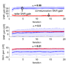
Figure 2: Convergence of SNR gains for radar and communication, $P_{R}=30$ dBm, $N_{T}=16$, $N=36$.

IV NUMERICAL RESULTS

In this section, we provide numerical results to show the trade-off between the radar and communication metrics by varying the weight factor for radar SNR ($\alpha$). In addition, the scalability of the two presented low-complexity algorithms, i.e. twice minorization [8] and RMO [9], are discussed.

Fig. 2 illustrates the impact of the weight factor $\alpha$ on the radar SNR. The convergence of the SNR gains for both radar and communication functions is also shown. The solid line denotes the SNR gain averaged over $50$ iterations, and the shaded area around the mean represents the variance among different realizations. The blue color is assigned to the radar metric, and the red to the communication metric. It is observed that, by decreasing $\alpha$ from $0.99$ to $0.01$, the radar SNR gain drops from around $30$ dB to around $0$ dB, and the communication SNR gain increases from around $0$ dB to around $7$ dB. This shows that the radar SNR is more sensitive, as compared to the communication SNR, the reason being that the former is a fourth order function of $\mathbf{\Phi}$, while the latter is a quadratic function of $\mathbf{\Phi}$.

Fig. 3 shows the average time to converge for the different algorithms considered. It is observed that the Riemannian manifold optimization [9] of Section III-B4, and the twice minorization [8] of Section III-B2, scale well with IRS size ($N$). This shows the benefit of the closed-form expression based solution update scheme, compared to numerical solvers based method, for problems with large size variable $(N)$.

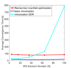
Figure 3: Average convergence time versus number of IRS elements ($N$), $P_{R}=30$ dBm, $N_{T}=16$, $\alpha=0.9$.

V CONCLUSIONS

In this paper, we have presented several methods of designing the IRS parameter matrix for IRS DFRC systems. The classical method is applying the MM technique to create a solvable quadratic programming. One low-complexity design is creating a linear surrogate objective function by using MM twice. Another low-complexity method is by using Riemannian manifold optimization directly on the original fourth order objective. In addition, branch and bound framework based design has been presented that achieves a near-optimal solution chosen from multiple iteratively obtained local optima.

References

- [1] B. Li, A. P. Petropulu, and W. Trappe, “Optimum co-design for spectrum sharing between matrix completion based MIMO radars and a MIMO communication system,” IEEE Trans. Signal Process., vol. 64, no. 17, pp. 4562–4575, 2016.
- [2] J. A. Zhang, F. Liu, C. Masouros, R. W. Heath, Z. Feng, L. Zheng, and A. Petropulu, “An overview of signal processing techniques for joint communication and radar sensing,” IEEE Journal of Selected Topics in Signal Processing, vol. 15, no. 6, pp. 1295–1315, 2021.
- [3] F. Liu, C. Masouros, A. P. Petropulu, H. Griffiths, and L. Hanzo, “Joint radar and communication design: Applications, state-of-the-art, and the road ahead,” IEEE Trans. Commun., vol. 68, no. 6, pp. 3834–3862, 2020.
- [4] Z. Xu and A. Petropulu, “A bandwidth efficient dual-function radar communication system based on a MIMO radar using OFDM waveforms,” IEEE Trans. Signal Process., vol. 71, pp. 401–416, 2023.
- [5] Q. Wu and R. Zhang, “Intelligent reflecting surface enhanced wireless network via joint active and passive beamforming,” IEEE Trans. Wireless Commun., vol. 18, no. 11, pp. 5394–5409, 2019.
- [6] ——, “Towards smart and reconfigurable environment: Intelligent reflecting surface aided wireless network,” IEEE Commun. Mag., vol. 58, no. 1, pp. 106–112, 2020.
- [7] S. Buzzi, E. Grossi, M. Lops, and L. Venturino, “Foundations of MIMO radar detection aided by reconfigurable intelligent surfaces,” IEEE Trans. Signal Process., vol. 70, pp. 1749–1763, 2022.
- [8] Y.-K. Li and A. Petropulu, “Minorization-based low-complexity design for IRS-aided ISAC systems,” arXiv:2302.11132, 2023.
- [9] Y. Li and A. Petropulu, “Dual-function radar-communication system aided by intelligent reflecting surfaces,” in 2022 IEEE 12th Sensor Array and Multichannel Signal Processing Workshop (SAM), 2022, pp. 126–130.
- [10] Z.-M. Jiang, M. Rihan, P. Zhang, L. Huang, Q. Deng, J. Zhang, and E. M. Mohamed, “Intelligent reflecting surface aided dual-function radar and communication system,” IEEE Syst. J., pp. 1–12, 2021.
- [11] R. Liu, M. Li, Y. Liu, Q. Wu, and Q. Liu, “Joint transmit waveform and passive beamforming design for RIS-aided DFRC systems,” IEEE J. Sel. Topics Signal Process., vol. 16, no. 5, pp. 995–1010, 2022.
- [12] Y. Sun, P. Babu, and D. P. Palomar, “Majorization-minimization algorithms in signal processing, communications, and machine learning,” IEEE Trans. Signal Process., vol. 65, no. 3, pp. 794–816, 2017.
- [13] M. Najafi, V. Jamali, R. Schober, and H. V. Poor, “Physics-based modeling and scalable optimization of large intelligent reflecting surfaces,” IEEE Trans. Commun., vol. 69, no. 4, pp. 2673–2691, 2021.
- [14] B. Li and A. P. Petropulu, “Joint transmit designs for coexistence of MIMO wireless communications and sparse sensing radars in clutter,” IEEE Trans. Aerosp. Electron. Syst., vol. 53, no. 6, pp. 2846–2864, 2017.
- [15] Z.-q. Luo, W.-k. Ma, A. M.-c. So, Y. Ye, and S. Zhang, “Semidefinite relaxation of quadratic optimization problems,” IEEE Signal Process. Mag., vol. 27, no. 3, pp. 20–34, 2010.
- [16] M. Grant and S. Boyd, “CVX: Matlab software for disciplined convex programming, version 2.1,” http://cvxr.com/cvx, Mar. 2014.
- [17] M. Soltanalian and P. Stoica, “Designing unimodular codes via quadratic optimization,” IEEE Trans. Signal Process., vol. 62, no. 5, pp. 1221–1234, 2014.
- [18] L. Wu, P. Babu, and D. P. Palomar, “Transmit waveform/receive filter design for MIMO radar with multiple waveform constraints,” IEEE Trans. Signal Process., vol. 66, no. 6, pp. 1526–1540, 2018.
- [19] F. Liu, L. Zhou, C. Masouros, A. Li, W. Luo, and A. Petropulu, “Toward dual-functional radar-communication systems: Optimal waveform design,” IEEE Trans. Signal Process., vol. 66, no. 16, pp. 4264–4279, 2018.