Directedeness, correlations, and daily cycles in springbok motion: from data over stochastic models to movement prediction

Abstract

How predictable is the next move of an animal? Specifically, which factors govern the short- and long-term motion patterns and the overall dynamics of landbound, plant-eating animals and ruminants in particular? To answer this question, we here study the movement dynamics of springbok antelopes Antidorcas marsupialis. We propose complementary statistical analysis techniques combined with machine learning approaches to analyze, across multiple time scales, the springbok motion recorded in long-term GPS-tracking of collared springboks at a private wildlife reserve in Namibia. As a new result, we are able to predict the springbok movement within the next hour with a certainty of about 20%. The remaining 80% are stochastic in nature and are induced by unaccounted factors in the modeling algorithm and by individual behavioral features of springboks. We find that directedness of motion contributes approximately 17% to this predicted fraction. We find that the measure for directedeness is strongly dependent on the daily cycle. The previously known daily affinity of springboks to their water points, as predicted from our machine learning algorithm, overall accounts for only 3% of this predicted deterministic component of springbok motion. Moreover, the resting points are found to affect the motion of springboks at least as much as the formally studied effects of water points. The generality of these statements for the motion patterns and their underlying behavioral reasons for other ruminants can be examined on the basis of our statistical analysis tools.

I Introduction

Ronald Ross, who received the 1902 Nobel Prize for Physiology or Medicine for his discovery on the transmission of malaria by mosquitoes, formulated the fundamental problem to understand the spatiotemporal spreading of infected mosquitoes from a breeding pool ross : "Suppose that a mosquito is born at a given point, and that during its life it wanders about, to and fro, to left or to right, where it wills, in search of food or of mating, over a country which is uniformly attractive and favorable to it. After a time it will die. What are the probabilities that its dead body will be found at a given distance from its birthplace?" To solve this problem, Ross contacted the statistician Karl Pearson, who is credited for creating the concept of the random walk. In an exchange of Letters in Nature with John William Strutt, Lord Rayleigh, it became apparent that after sufficiently many steps the position of the random walker converges to a Gaussian random variable pearson ; rayleigh ; pearson1 ; benh08walks ; hughes . In fact, the random walk is close to Einstein’s and Smoluchowski’s formulations of the mathematical theory of diffusion einstein ; smoluchowski , and generalizations of this simple concept have been extensively used in the modeling of how animals search for resources.

A milestone towards modern movement ecology were animal counts and the tracking of their seasonal migration patterns by aerial observation in the late 1950s, informing authorities on the best layout for the newly established Serengeti National Park in Tanzania, Africa. Today, several well-developed methods to record the movement of animals are routinely employed benson . We mention GPS tracking of transmitting tags gps ; gps1 ; jelt22 and automated radio tracking, particularly, the high-throughput ATLAS (Advanced Tracking and Localization of Animals in real-life Systems) atlas ; atlas1 . The observations garnered by such methods are at the core of movement ecology, an emerging unifying paradigm for understanding the various mechanisms underlying animal behavior and the consequences for key ecological and evolutionary processes nath08para ; Nathan22 . Thus movement ecology builds on early theoretical ideas of dispersal in populations pear06 ; skel51 and the connection with epidemic spreading brow12epid . Classes of interest in movement ecology based on individual tracking of organisms include, i.a., mammals jelt22 ; tuck18 , birds assa22prx ; vilk ; atlas1 ; jelt16storks , bats roeleke22 , or marine predators sims08 ; sims11 . A key question is to predict the "next move" gura16tortous of an animal with some statistical certainty.

Unveiling a broader picture in the movement ecology of even a single species is hampered by various factors, including effects of seasonal changes of animal behavior and the environment, migration, reproduction cycles and breeding, intra-species collective phenomena and group size, interactions with foreign species, variations of behaviors and physiology between individuals, heterogeneity of the environment and resources, home-ranging and confinement, among a variety of other factors. The original expectations that relatively simple stochastic models could capture essential features of movement ecology therefore have remained elusive, and most models are species-specific. While a universal modeling framework may be unattainable, a central longer-term question is whether we can identify universal dynamic modules, which occur for broad ranges of species.

Several stochastic models have been used to describe the movement patterns of animals, starting with the normal random walk (Pearson walk) mentioned above for the description of mosquito spreading and applications to crabs pear06 and muskrats skel51 . While a random walk is a Markovian process and the direction of each jump independent of the previous jump, a direct generalization is represented by correlated random walks with a finite correlation time (typically modeled with Ornstein-Uhlenbeck noise or by coupling to a diffusive rotational motion of the direction of motion) fuer20 ; kare83 ; visw05corr ; benh08walks ; romanczuk2012 ; gura17corrvelo ; elisabeth . Beyond the correlation time, such processes are normal-diffusive with an effective diffusivity romanczuk2012 . Once the correlations are taken to be long-range, such as in fractional Brownian motion with positive, power-law correlations of the driving Gaussian noise mandelbrot , the resulting motion is superdiffusive with a mean squared displacement (MSD) of the form $\langle\mathrm{r}^{2}(t)\rangle\simeq t^{\alpha}$ and $1<\alpha\leq 2$ report ; metz14 ; soko15 . Crossovers from superdiffusive power-law forms of the MSD to normal diffusion or another power-law can be achieved by different forms of tempering of the driving noise daniel . In the standard formulation of these models the motion is unbounded. Finite domains such as home ranges or confinement by geographic boundaries or fencing can then be included by appropriate boundary conditions or introduction of a confining potential. In such cases the motion will eventually reach a non-equilibrium steady state (NESS) characterized by a stationary probability density function (PDF). A NESS can also be reached by so-called random resetting strategies, in which an a priori unbounded stochastic process such as Brownian motion is "reset" back to its origin (or to another point with a given probability marcus ; shlomi ), typically following a Poisson statistic of reset times satya ; evansreview . Resetting has been generalized to a large number of stochastic processes, we only mention some representative examples activereset ; reset1 ; reset2 ; trifce ; trifce1 ; andrey ; andrey1 ; chechkin ; chechkin1 .

In the context of random search for sparse food a long debate has focused on "optimal search" olivierreview ; searchreview . Intermittent search strategies olivier ; olivier1 ; gandhi ; michael ; vladinter combine local search, typically Brownian motion, with a persistent process such as ballistic motion. The role of the latter is to decorrelate the searcher by relocating it to a remote area, that likely has not been visited before. A second strategy to reduce oversampling in one and two dimensions are Lévy search processes, in which relocation lengths are power-law distributed, such that hierarchical clusters are searched mandelbrotbook ; shlekla . This reduces the search time shlekla ; michael ; michaelprl . The Lévy flight foraging hypothesis gandhi led to a large number of studies identifying Lévy patterns in animal motion visw96 ; visw99 ; stan07 ; sims12 ; Gurarie09 ; gura22 ; boye06 ; boye14 ; sims08 ; hump10tuna ; visw10 ; sims11 ; jage11 ; foca17 ; kare83 ; hirt22 ; mura20bugs and in human motion patterns raic14human ; brockmann ; talkoren ; havlincovid . While in some cases the Lévy model has been questioned pyke15 ; stan07 ; trav07 ; edwa12 ; paly14levy , it focused the interest of the statistical physics community on movement ecology.

Obviously, while simple random search models may provide essential insight into observed motion patterns, they cannot capture the full complexity displayed by higher animals and thus represent a starting point for further analysis. To develop better models in movement ecology, various other effects need to be considered, e.g., spatial memory faga13 , task-optimized navigation strategies panzachhi2015reindeer , food abundance CHEN202215 , group dynamics roeleke22 , information exchange between sub-populations in a community jelt20rev-commun ; roeleke22 , heterogeneity of the terrain, habitat-connectivity panzachhi2015reindeer , or selection potts2020diffssa . We here propose dedicated statistical analysis techniques in combination with machine-learning (ML) approaches, to study to which degree these tools can be used towards predicting the movement patterns of ruminants depending, inter alia, on daily and annual cycles, on resource distribution in the home range, on area restriction due to confinement, and on additional features, that can only be described in a statistical way. We validate these methods to analyze long-term GPS-tracking data of springboks in a private wildlife reserve in Namibia on various time-scales. We show that our approach helps us to understand the limitations, but also some important features of springbok motion which can be generalized to the description of motion patterns of other ruminant species inhabiting semi-arid landscapes. Moreover, the concepts developed here are promising to be applied on a more generic level to analyze and predict movement patterns of higher animals.

The structure of the paper is as follows. We introduce the data set for our study in Sec. II and characterize it by applying stochastic modeling in Sec. III. In Sec. IV we focus on two main questions, the importance of water point positions for the overall dynamics of springbok movement and how the directedness benh04-tortuos-straight of gazelle motion and their activity depend on the hour of the day. Finally, in Sec. V we discuss the forecasting power of the ML-based models in dependence on input features such as season, water point distance, and vegetation levels. We conclude our investigation in Sec. VI.

II Data acquisition and visualization

The movement patterns of medium-sized ruminants such as antelopes, gazelles, and springboks have been intensely investigated walt68 ; Bigalke1970 ; bigalke1972 ; davi78 ; skin96 . While earlier studies relied on extensive direct observations such as aerial monitoring or radio tracing by handheld antennae, automated contemporary tracking methods allow scientists to garner high-resolution, long-time tracking data. An extensive range of behavioral details has been revealed, including activity rhythms, seasonal influence, water needs, gaits, feeding habits and preferences including, social habits, reproduction cycles, lambing peaks, herd composition, age-related changes, sex-specific behavior, body-weight distribution, etc. Bigalke1970 ; bigalke1972 ; davi78 ; walt68 .

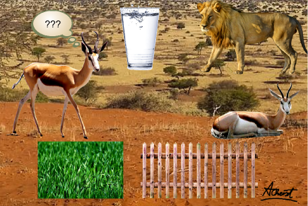
Figure 1: Illustration of some vital daily decisions of a springbok, to choose the best survival, foraging, resting, etc. strategies of movement. Courtesy www.pixabay.com for the source images and to Alexey A. Cherstvy for preparing the artwork.

In the current study, female Antidorcas marsupialis (springboks) were equipped with e-Obs GPS collars heringdon for tracking. These animals have a shoulder height of approximately 80 cm and weight between 30 to 40 kg. They can reach speeds of up to 88 km/h in extended gallop bigalke1972 . An image of a springbok together with its decision options is shown in Fig. 1.

Each collared individual was selected from a different herd during the dry season and can thus be treated to move independently from other tracked individuals. The study area was located between the regions of Kunene, Omusati, and Oshana in the north of Namibia, at $15.2235^{\circ}\mathrm{E}$, $19.2576^{\circ}\mathrm{S}$, approximately 80 km south-west of the Etosha pan, at Etosha Heights Private Reserve and Etosha National Park. The vegetation zones in Etosha Park are known to be very diverse, depending on the soil properties and water abundance. Rainfall in the study area is highly variable, but mainly occurs from October to April. During this wet season the mean daily temperature is around $26^{\circ}\mathrm{C}$, with daily variations of some $15^{\circ}\mathrm{C}$. The dry season is somewhat colder, with mean temperatures around $18^{\circ}\mathrm{C}$ and daily variations of around $20^{\circ}\mathrm{C}$. Our data set contains the positions of eight springboks taken at time intervals of $\Delta t=15$ min for up to 31 months. The focal landscape is confined by a fence, which happens to be damaged at places and thus allows some animals to cross or jump over it. Detailed information on how animals interact with fences and on their energy expenditure is available for female Antidorcas marsupialis (springbok), Tragelaphus oryx (eland), and Tragelaphus strepsiceros (kudu) heri22fence .

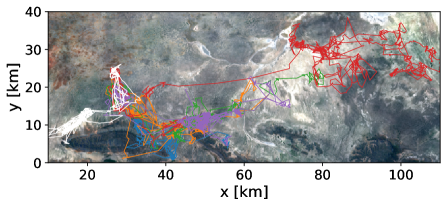
(a) (b)

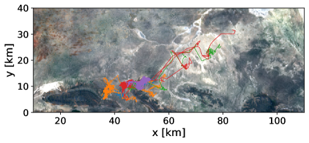
Figure 2: Movement data of all springboks in the data set during (a) the wet season of 2019/2020 and (b) the dry season of 2020. Different colors denote distinct animals.

The average precision of the GPS positioning of the GPS-tagged springboks was quite high because the weather conditions and the vegetation structure were ideal for satellite reception. Each single position in the data set corresponds to an average of a sequence of five GPS records taken at one second intervals. When not moving (one GPS-sensor was tracked while laying in the field) the apparatus yielded an accuracy of about $\delta x_{\mathrm{err}}\approx 2\mathrm{m}$ in two-dimensional position acquisition. Some pre-processing of the data was conducted. Thus, missing data points (if only up to one hour of data was missing) were replaced with the previous values of the animal’s position. Position data were stored along with the underlying vegetation pattern from the data set and with the recorded ambient temperatures.

Springbok movement data during the wet and dry seasons are displayed in Fig. 2. We observe that during the dry season the motion of the animals is more localized around the water points, as the environmental conditions necessitated regular returns to the water points for re-hydration. The statistic of consecutive turning angles of all tracked springboks is illustrated in wind rose diagrams in Fig. 3. Visually (see below for details) short-time persistent motion in the same direction on 15 min intervals is distinct. Quite pronounced antipersistence is seen on the daily time scale, signifying the eventual return to some preferred location every day.

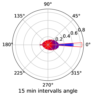
(a) (b)

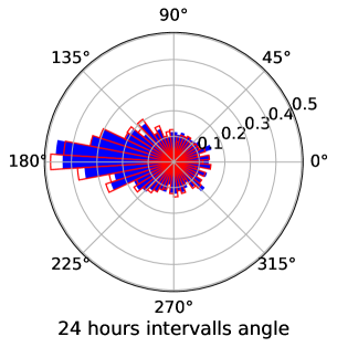
Figure 3: Histograms of the turning angles between two successive steps of springbok movement (data from all individuals), for data processed with (a) 15 min time steps and (b) one-day time steps. The full dataset (blue fill) is shown together with the dry season data only (red outline).

III Stochastic modeling

There exist a substantial number of both theoretical and data-based studies dealing with animal motion modeling, see, e.g., BOVET1988419 ; Gurarie09 . Typical observables are the moments of the motion or the corresponding position or displacement autocorrelations. Correlations (persistence) in the motion is an expected feature for directedness, and it may be associated as some measure for the intelligence of the forager bhat2022smart . Single trajectory power spectral analyses may be additional quantities for analysis prx ; vilkjpa . To describe the observed two-dimensional springbok motion we start with a simplistic two-dimensional Brownian motion, that we write in the discrete form

$$\mathbf{r}(t_{i})=\mathbf{r}(t_{i-1})+\xi(t_{i})\mathbf{e}_{\varphi}(t_{i}),$$ (1)

where $\mathbf{e}_{\varphi}(t_{i})=(\sin(\varphi(t_{i})),\cos(\varphi(t_{i})))$ and $t_{i}=i\Delta t$ is the time expressed in terms of elementary time steps $\Delta t$, see below. The Gaussian driving longitudinal noise $\xi$ is of zero mean and has the autocovariance function (ACVF) $\langle\xi(t_{i})\xi(t_{j})\rangle=2K\delta_{ij}\Delta t$, where $\delta_{ij}$ is the Kronecker delta. Moreover, $K$ is the diffusion coefficient. The noise impulse $\xi(t_{i})$ is allocated to the two Cartesian co-ordinates via the random angle $\varphi(t_{i})$, assumed to be uniformly distributed on $[0,\pi)$. The MSD of this process then becomes

$$\langle\mathbf{r}^{2}(t_{i})\rangle=4Kt_{i},$$ (2)

with $|\mathbf{r}(t_{i})|=\sqrt{x^{2}(t_{i})+y^{2}(t_{i})}$ and the initial condition $x(0)=y(0)=0$. The angular brackets $\langle\cdot\rangle$ denote averaging over realizations of the noise $\xi$. We note that on a log-log scale the MSD thus has unit slope. From an individual time series $\mathbf{r}(t_{i})$ of $N$ steps we calculate the time-averaged MSD (TAMSD)

$$\overline{\delta^{2}(\Delta_{l})}=\frac{1}{N-l}\sum_{i=1}^{N-l}\left(\mathbf{r}(t_{i+l})-\mathbf{r}(t_{i})\right)^{2},$$ (3)

in terms of the "lag time" $\Delta_{l}=l\Delta t$ pt . As Brownian motion is self-averaging, when $l\ll N$ we have

$$\overline{\delta^{2}(\Delta_{l})}=4K\Delta_{l},$$ (4)

that is, the process is ergodic in the Boltzmann-Birkhoff-Khinchin sense pt ; pnas . In the following we drop the indices for discrete times, for convenience.

(a)

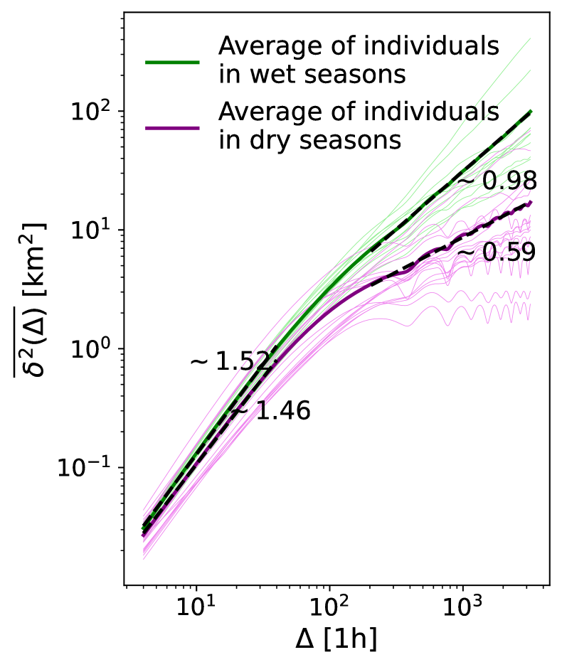
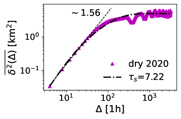
(b) (c)

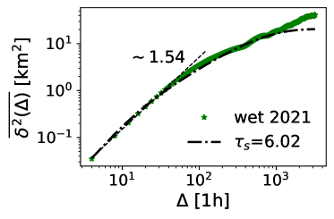
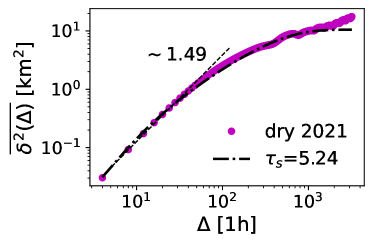
(d) (e)

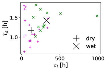
Figure 4: (a) TAMSDs of springbok movement data with time steps of 15 minutes for all individuals in all seasons. The thick lines are averages for all TAMSDs from the the wet season and the dry season, respectively. The traces of each animal were divided into wet and dry seasons, so that the total number of (partial) trajectories is about three times larger than the number (8) of individual animals in the data base. The slopes of the average TAMSDs for small and large $\Delta$ are indicated by the fitted scaling exponents. The oscillations in the TAMSD observed at intermediate-to-long lag times with a period of 24 h are due to repetitive returns to certain preferential points, such as favorite water and/or resting points. (b-d) TAMSDs for dry (b,d) and wet (c) seasons for the same individual; the dashed line shows the small $\Delta$ scaling; the theoretical expression (9) with free parameters $\tau_{s}$, $\tau_{l}$, and $K$ is fitted and shown as the dashed-dotted line: Note that the oscillations in the dry-season TAMSD curve (b) at intermediate to long times are artefacts of the daily cycle. (e) Fitted model parameters: the short and long time scales $\tau_{s}$ and $\tau_{l}$ are compared for different individuals during dry and wet seasons, see the legend and Eq. (9) for details. Both characteristic times are longer during the wet season in comparison to those during the dry season, the difference is more significant for $\tau_{l}$.

Individual experimental TAMSDs of a number of individual springboks are shown in Fig. 4a for wet and dry seasons, respectively, along with the averages for each springbok ensemble. We see that the initial slope is greater than unity, reflecting superdiffusive motion. As we will see, this superdiffusion is due to persistence in a given direction of motion. After lag times of some 70 to 100 h the slope of the TAMSD changes, corresponding to traveled distances of some 1 to 2 km. While for a number of trajectories the TAMSD continues to grow, with a larger slope $\alpha\approx 0.98$ during wet seasons as compared to $\alpha\approx 0.59$ during dry seasons, the TAMSD for some other trajectories flattens off to a plateau value at around 100 h. Such a plateau value within the measured lag time window appears more often in dry than in wet seasons. We note that even for those animals, whose TAMSD grows until the maximum lag time displayed in Fig. 4a, the TAMSD eventually also reaches a plateau a fortiori, as the habitat is finite. Moreover, we point out that even for the data points at shorter times (smaller distances) the contribution $\delta x_{\mathrm{err}}^{2}$ to the TAMSD due to measurement error is negligible, and thus the extracted scaling exponents of the TAMSD are meaningful. We conclude from these observations that the simple model of Brownian motion with TAMSD (4) is insufficient to account for the data. Instead, we are seeking a model that captures the initial superdiffusion $\overline{\delta^{2}(\Delta)}\simeq\Delta^{\alpha}$ with $\alpha>1$, a crossover to a second scaling regime $\overline{\delta^{2}(\Delta)}\simeq\Delta^{\alpha^{\prime}}$, and a terminal plateau behavior, $\overline{\delta^{2}(\Delta)}\simeq\mathrm{const}$.

Let us first address the confinement effect. As an approximation we assume that the animal motion is subject to an harmonic potential. Such a "soft" confinement, in contrast to "hard" confinement in a finite box or in higher order potentials such as $x^{4}$ forms, allows for variations in the maximal traveled distance. These variations may occur, for instance, when the animal ventures out further when a fence is broken or during periods of lusher vegetation. Discrete Brownian motion in an harmonic confinement is then described by our discrete-time Langevin equation (1) with damping coefficient $\exp(-\Delta t/\tau_{l})$ ghosh ; miao ; qin ,

$$\mathbf{r}(t_{i})=e^{-\Delta t/\tau_{l}}\mathbf{r}(t_{i-1})+\xi(t_{i})\mathbf{e}_{\varphi}(t_{i}),$$ (5)

This formulation is equivalent to the autoregressive model AR(1) of order one Box15 , representing the discrete version of the seminal Ornstein-Uhlenbeck (OU) process orns17 ; uhle30 ; risken ; cher18ou . The time scale $\tau_{l}$ in the exponential prefactor in Eq. (5) is the characteristic correlation time induced by the harmonic potential. At short times, the TAMSD of the process (5) is linear in time, while at long times the TAMSD converges to $4K\tau_{l}$ meyer2022ho .

In the short-time limit, the OU process with its linear scaling in time is thus not an appropriate model for the observed springbok movement. Instead, animal movement is characterized by a certain degree of persistence, i.e., the trend to keep moving in a given direction romanczuk2012 ; gv , as indicated by the angle histograms in Fig. 3. There are different modeling approaches in literature for such persistence. As mentioned above, random search by animals is often described by Lévy flights or walks. Due to the long tailed jump length distributions, they perform superdiffusion. Lévy flights in harmonic potentials lead to mono-modal (with a single maximum at the origin) stable PDFs sune , while in steeper than harmonic potentials their PDFs exhibit bi-modal structures (with maxima away from the origin) chech ; chech1 ; karol . Lévy walks with long-tailed jump distributions but a finite propagation speed exhibit bi-modal PDFs already for harmonic confinement pengbo , including scenarios, in which the harmonic potential is only switched on stochastically ("soft resetting") pengbo1 . Alternatively, superdiffusive animal motion can be described by fractional Brownian motion (FBM) vilk , defined in terms of a Langevin equation driven by power-law correlated Gaussian noise mandelbrot . Positively correlated FBM in steeper than harmonic potentials also exhibits bi-modal PDFs tobias ; tobias1 .

Here we will use a minimal model to introduce confinement and persistence without long-range jump length distributions of power-law displacement correlations. Namely, we will show that the springbok movement data can be nicely described by replacing the white noise $\xi$ in Eq. (5) by exponentially correlated noise $\mathbf{z}$ maggi ; fodor ,

$$\mathbf{r}(t_{i})=e^{-\Delta t/\tau_{l}}\mathbf{r}(t_{i-1})+\mathbf{z}(t_{i}),$$ (6)

where we choose

$$\mathbf{z}(t_{i})=e^{-\Delta t/\tau_{s}}\mathbf{z}(t_{i-1})+\sqrt{\frac{\Delta t}{\tau_{s}}}\xi(t_{i})\mathbf{e}_{\varphi}(t_{i}).$$ (7)

Here $\xi$ is white Gaussian noise and $\tau_{s}$, chosen as $\tau_{s}\ll\tau_{l}$, is the correlation time of the driving noise $\mathbf{z}$. Comparing with Eq. (5) it is clear why the noise $\mathbf{z}$ is often called OU noise. These equations can be simplified by eliminating $\mathbf{z}$, yielding the autoregressive process AR(2) of order two Box15 ,

$$\mathbf{r}(t_{i}) = (e^{-\Delta t/\tau_{l}}+e^{-\Delta t/\tau_{s}})\mathbf{r}(t_{i-1})$$ (8)

$$-e^{-\Delta t/\tau_{l}-\Delta t/\tau_{s}}\mathbf{r}(t_{i-2})+\sqrt{\frac{\Delta t}{\tau_{s}}}\xi(t_{i})\mathbf{e}_{\varphi}(t_{i}).$$

The TAMSD defined by the model (8) reads meyer2022ho

$$\left<\overline{\delta^{2}(\Delta)}\right>=\frac{4K\tau_{l}^{2}}{\tau_{l}^{2}-\tau_{s}^{2}}\left[\tau_{l}\left(1-e^{-\Delta/\tau_{l}}\right)-\tau_{s}\left(1-e^{-\Delta/\tau_{s}}\right)\right].$$ (9)

In the short time limit $\Delta\ll\tau_{s}$, this expression encodes the ballistic scaling

$$\left<\overline{\delta^{2}(\Delta)}\right>\sim\frac{2K\tau_{l}}{\tau_{s}(\tau_{l}+\tau_{s})}\Delta^{2},$$ (10)

whereas at intermediate times $\tau_{s}\ll\Delta\ll\tau_{l}$ we find a linear $\Delta$-dependence with a correction term,

$$\left<\overline{\delta^{2}(\Delta)}\right>\sim\frac{4K\tau_{l}^{2}}{\tau_{l}^{2}-\tau_{s}^{2}}\left(1-\frac{\Delta}{\tau_{l}}\right)\Delta.$$ (11)

At long times, $\Delta\gg\tau_{l}$, the TAMSD reaches the plateau value

$$\left<\overline{\delta^{2}(\Delta)}\right>\sim\frac{4K\tau_{l}^{2}}{\tau_{l}+\tau_{s}}.$$ (12)

The characteristic times $\tau_{s}$ and $\tau_{l}$ describe the dominant dependencies of the TAMSD in the limts of short and long times, respectively (as indicated by the indices). We use the TAMSD to assess the typical ballistic and confined motion (converging to a plateau) of sprtingboks expected at short and long times.

The solution (9) can be fitted to the measured TAMSD of the springbok data. As we can see in Fig. 4b the agreement is quite good. At shorter times we see that the model with the three fit parameters $K\sim 1\ldots 10\mathrm{km}^{2}/\mathrm{h}$, $\tau_{s}\sim 1\mathrm{h}$, and $\tau_{l}\sim 1\mathrm{day}$, matches the data well up to the time scale of a week, and levels off to the plateau somewhat too early. However, given that the initial power-law regime spans merely around one decade, this does not appear too severe. In contrast, we believe that the relatively simple AR(2) model allows for easy physical interpretation of the parameters and provides a very satisfying description (for more details see the data sections below). Importantly, in this AR(2) model we can easily include an error analysis relevant for experimental data.

Before we continue we briefly describe our fitting procedure of TAMSD curves as those shown in Fig. 4b. We use a nonlinear fit of the TAMSD (9), equivalent to a nonlinear fit to the fluctuation function meyerDFA . The model has three free parameters $K$, $\tau_{l}$, and $\tau_{s}$. The fact that the most reliable points of the TAMSD are those at shorter lag times while most points are available at longer times (due to the logarithmic scaling) makes the fit challenging. The solution we choose is to fit one parameter at a time. For the fit shown in Fig. 4b we therefore practically divide the lag time window into separate intervals and fit the time scales to the relevant range of lag times. This is possible as long as $\tau_{l}\gg\tau_{s}$, which we obtain from the data self-consistently. We start measuring the variance $\sigma^{2}$ (related to the diffusivity $K$) of the time series. As the curvature of the TAMSD is independent of $\tau_{s}$ for $\Delta\gg\tau_{s}$, we set $\tau_{s}$ to a small value and fit $\tau_{l}$ in the range between $1.25$ h and 3.75 h. Finally, $\tau_{s}$ is fitted using the parameters $K$ and $\tau_{l}$, and the first two points of the dataset.

The results are displayed in Fig. 4. In panel (a) we show all seasons and individuals along with the average for each season. Panels (b-d) are examples from one individual during three different seasons. In Fig. 4c we show all measured parameters $\tau_{s}$ and $\tau_{l}$ of different animals during movement in both wet and dry seasons. Generally, $\tau_{l}$ is larger in the wet season, reflecting a confinement of animals due to a lack of resources during the dry season. The time scale $\tau_{s}$ also has a tendency to be smaller in dry seasons. There is, however, a large overlap in the found distributions of $\tau_{s}$ and $\tau_{l}$ when comparing seasons. In all situations the strong inequality

$$\tau_{l}\gg\tau_{s}$$ (13)

holds, so that in the short-time limit the dynamics of animals can be approximated by free diffusion with correlated driving $\zeta$.

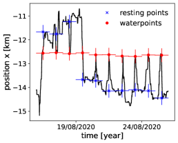
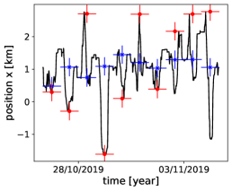
a) b) c)

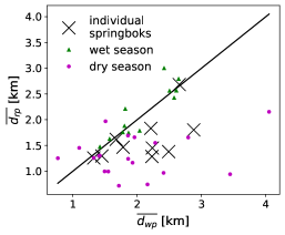
Figure 5: Effects of water and resting points. (a) Segment of the trajectory $x(t)$ (position time series projected onto the $x$ direction) during which the springbok visits the same water point every day, while the maximum distance and the resting points vary. (b) Segment of another trajectory, during which the resting point remains almost constant while the animal visits different water points. (c) Mean distance between the resting points on two subsequent days versus the distances of visited water points on subsequent days. Large crosses are calculated for the full data set of single individuals. The small symbols are from the same data sets, but averages are taken only over the 6 months of either dry or wet season, see legend. The black line represents the diagonal.

IV Feature characteristics

The above model takes into account finite-time correlations in the movement and confinement. We here discuss the influence of two important additional features, namely, geographical features such as water and resting points, and temporal features such as day and night.

IV.1 Water and resting points

Water points are a key element in springbok movement dynamics. Although springboks are well adapted to arid environments and can survive long periods without drinking skin96 , they regularly visit water points when available. This way, they avoid negative physiological consequences during the adjustment to a low water supply Cain2006spwater . Springboks drink at water points throughout day time but also occasionally during night time bigalke1972 . To understand the springbok movements it is necessary to investigate the effects of water points.

During the wet season, when there is ample nutritious food available, it is known that large herds of hundreds of springboks concentrate on open, highly productive grassland bigalke1972 . During the dry season, when food is more limited, the springboks disperse and form smaller groups of a few dozen of individuals bigalke1972 . Such behavior may, however, vary between different areas davi78 ; Roche2008 and largely depends on the combined environmental factors such as water point location and their water levels, fencing, general geo-hydrology, weather, and other. The behavior with respect to the water holes is not unique, as shown in Fig. 5a,b. The segment of the animal trajectory shown in panel (a) shows a preferential return to the same water point while different resting points are chosen and the animal has a fairly constant maximal range of motion on consecutive days. In contrast, in the trajectory segment in panel (b) the same individual covers much smaller daily distances (roughly 10% of the covered spans of panel (a)), and shows only small variations in the resting points, while it visits continuously changing water points.

The springbok resting points at night correspond to the maximum of their temporal occupation density, i.e., the local area where they spend most time in a 24 hour span. In some periods, the resting points of animals are almost the same every night, see Fig. 5b, while in other cases the resting points are more distant (panel (a)). In order to find the maximum of the probability density of springbok positions on a specific day, one approach is to recursively delete the point which is furthest away for the median. This way we start with the full set $\{x(T),y(T)\}$ of positions of length $24\times 4$ for all recorded positions during the span of a single day ($T$ runs from midnight to 23:45 hours). We then enumerate the distance $([x(T)-\mathrm{median}(x(T))]^{2}+[y(T)-\mathrm{median}(y(T))]^{2})^{1/2}$. The elements $\{x(T_{\mathrm{max}}),y(T_{\mathrm{max}})\}$ which has the maximal distance from the median of $x$ and $y$ is then deleted, and the procedure is repeated with the next point, until only one point is left in the set. This identifies the maximum of the probability density.

To quantify the effects of water and resting points on the springbok movement, we define, for each day, the point closest to a water point as $\{x_{\mathrm{wp}},y_{\mathrm{wp}}\}$ and the resting point, at which the density of the visited positions of the animal reaches a maximum, as $\{x_{\mathrm{rp}},y_{\mathrm{rp}}\}$. This is a somewhat crude approximation, because springboks do not necessarily visit a water point only once per day and do not have a single sleeping phase per day. However, the two sets of data points $\{x_{\mathrm{wp}},y_{\mathrm{wp}}\}$ and $\{x_{\mathrm{rp}},y_{\mathrm{p}}\}$ are, as we show, meaningful quantities for analysis.

We compute the mean distance of subsequent daily water or resting points as

$$d_{\mathrm{wp}}(T_{i}) = \Big{(}[x_{\mathrm{wp}}(T_{i})-x_{\mathrm{wp}}(T_{i}-1)]^{2}$$ (14)

$$+[y_{\mathrm{wp}}(T_{i})-y_{\mathrm{wp}}(T_{i}-1)]^{2}\Big{)}^{1/2},$$

where $T_{i}$ is the sequence of days. Analogously, we evaluate $d_{\mathrm{rp}}(T_{i})$ for the resting points. The mean of these expressions for different individuals in the tracked ensemble are compared in Fig. 5c. We find that, in general, the resting point distances vary less than those of the water points do. The analysis separating wet and dry seasons shows that the difference in variation is mostly due to the movement in the wet seasons, while in the dry seasons both time series vary similarly. The fact that longer journeys are necessary to find sufficient water supplies in the dry season reflects the expected conditions in arid climates. On average, therefore, we conclude that springboks rather keep to more localized resting points and travel further for water points.

A video of the motion of a springbok on an actual map with a variable vegetation index is presented in Fig. 6, together with motion-step predictions from our theoretical model (see below). Note that the modeled springbok is always somewhat lagging behind the actual measured springbok positions because predictions are weighted averages over all possible outcomes and, therefore, 2D-predictions tend to have somewhat smaller steps as compared to the true step lengths. The overall reproducibility of the movement directions, the magnitude of the turning angles, and the "intensity" of motion is, however, remarkable for the two springboks chosen from the dataset.

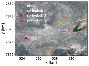
Figure 6: Snapshot from a movie of the motion of two springboks: the water points are marked as blue stars on the map, the actual animal positions are the orange and violet filled circles. The model predictions (for the same time intervals between steps) are denoted by the red crosses. The full movie file is provided in the Supplementary Material sm .

IV.2 Day- and night-autocorrelation

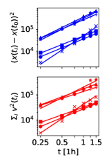
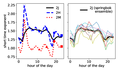
a) b) c)

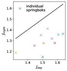
Figure 7: Displacements and short time scaling exponents of the ACVF of springbok motion. (a) Single springbok data, top: Scaling of the squared displacements along the trajectory for different hours of the day; bottom: cumulative sum of the squared velocities of springbok motion for different hours of the day. The different symbols represent different starting hours. We observe a spread in values of the scaling exponents depending on the time of day. (b) Springboks ensemble data, left: for each hour of the day, the average scaling exponents $\{2J,2H,2M\}$ are calculated as an average over days, using 15 min intervals. The symbols correspond to the ones used in panel (a). Exponents are disentangled following Eq. (16); right: for the long-range correlation exponent $J$, thin lines represent different individuals, the thick line is an average over all individuals. (c) Correlations between the scaling exponents $J$ during the day and night. Average scaling during the day (4 am to 6 pm) and night (6 pm to 4 am) shows a variability among the individuals and an increased directedness (i.e., more positive $J$ values) during the day for all animals in the dataset. The black line represents the diagonal.

We now address the dynamics encoded in the movement data on the level of a single day. The data segments shown in Fig. 5 suggest some daily cycle regarding the distances covered by the springboks. In this section we address the question whether this daily cycle in walked distance is due to a daily cycle in activity or due to a daily cycle in directedness of the motion or both. To this end, we need to assess all three quantities, the total distance, the activity and the directedness. With changing activity, we mean non-stationarity of the driving, related to the parameter $K$. Here, by directedness we mean short-time autocorrelations. One difficulty in distinguishing these two characteristics is the fact that our data has the resolution of only 15 min and thus shorter correlation times cannot be resolved. First, we need an assumption regarding the shape of short-time autocorrelations prior to starting the analysis. From Fig. 4(a-d) it follows that a power-law shape is a reasonable assumption for the short-time behavior of the TAMSD, which is closely related to the autocorrelation function meyer18 ; meye21moses ; meye22moses . So, for simplicity, we assume a power-law TAMSD scaling with a corresponding exponent in the short-time limit of the displacement. The total distance walked by an individual can be measured by the squared displacement $r^{2}_{h}(t)=(x_{h}(t)-x_{h}(0))^{2}+(y_{h}(t)-y_{h}(0))^{2}$, where the index $h$ denotes the time of the day when the measurement is started, and $r_{h}(0)$ is the starting position. One question is whether the growth of the squared displacement depends on the starting time, i.e. the hour $h$ of the day. Fig. 7a displays the average over an ensemble of days in the data set (we assume that the days can be considered independent). At each time of the day, we can assign a Hurst exponent $H$ to the ensemble-averaged displacement $\langle r_{h}^{2}(t)\rangle$, compare Eq. (17). As described in App. A, we also define scaling exponents for the velocity autocorrelation function (Joseph exponent $J$), and of the non-stationarity (Moses exponent $M$). The latter can be defined via the scaling of the cumulative squared increments of animals in $x$ and $y$ directions, i.e.

$$\left<\sum_{i=1}^{n}\mathbf{v}^{2}(t_{i})\right>\propto n^{2M+1},$$ (15)

with increments $\mathbf{v}(t_{i})=[\mathbf{r}(t_{i})-\mathbf{r}(t_{i-1})]/\Delta t$. It can be shown that the exponents $H$, $M$, and $J$ are related to each other via the following relation mand68moses ; che17 ; meyer18 ; aghion2021moses ; vilk

$$J=H-M+1/2,$$ (16)

as in our case due to the finite variance of the increments the Noah exponent $L=1/2$ (see also App. A).

Given relation (16), it is sufficient to calculate two of the three exponents for a certain hour of the day for the springbok motion to know all three of them. As the inference of autocorrelations usually involves time-averaging, we restrict ourselves to calculating the exponents $H$ and $M$. Here $M$ is defined by relation (15) and $H$ is defined by the ensemble-averaged MSD meyer18 ; meye21moses ; meye22moses ,

$$\left<(\mathbf{r}(t_{i})-\mathbf{r}(t_{0}))^{2}\right>\propto(t_{i}-t_{0})^{2H}.$$ (17)

In Eqs. (15) and (17) the brackets denote averaging over different days of springbok data and for each day $t_{0}$ corresponds to the same hour of the day. Using segments of length 90 min, we extract the short-time exponents.

In Fig. 7b,c we show the results of the computations for different times of the day and for different springboks. Figure 7b demonstrates the evolution of the short-time scaling exponents $\{J,H,M\}$ for all individuals measured at each hour of the day. The exponents $H$ and $M$ peak in the morning, reflecting the activity increase of the springboks increases fast as the sun rises. Note, that the exact time of the sunrise varies for each calendar day, but due to the location of springbok trajectories close to the equator this effect is relatively minor.

In Fig. 7c we plot the average exponent $J$—describing the directedness of the motion—during the day (4 am until 6 pm) versus the exponent computed during the night (6 pm until 4 am). We find that autocorrelations—quantified by the value of exponent $J$—during the day are more pronounced as compared to those during the night. During the entire day, the motion is more persistent than a completely random process ($2J>1$), but less directive/persistent than a ballistic process ($2J<2$).

We stress here that the underlying assumption of the existence of the power-law TAMSD scaling is a strong approximation and thus the inferred exponents are to be treated with care. According to Fig. 4b, the TAMSD$(\Delta)$ has a concave shape and thus autocorrelations in reality might somewhat higher at very short time-scales (that is below the time resolution of the current analysis (assuming power-laws)). The inferred influence of the autocorrelations can, therefore, be regarded as a lower bound to the impact of autocorrelations.

We find that changes in both activity and directedness contribute to the daily cycle. Both are not accounted for by model (8).

V Predictability

The analysis in the previous Section demonstrates that our relatively simple Ornstein-Uhlenbeck model (8) with correlated noise cannot fully describe all features of the springbok movement dynamics. While this simple model captures several essential features of the dynamic, it would be naive to expect that such rather generic physics-inspired models could grasp the complexity of effects such as day-night or seasonal variations. One possible generalization could include different parameters for day and night. The heterogeneity of the springbok movement stems from the environment or terrain features, but also from different modes of individual animal movement (such as, generally, hunting, resting, hiding, vigilance, etc.). Some studies specifically focus on classifying these modes of motion clintock2018hmm ; patin2020segclust2d ; bhat2022smart . Here we discuss some possible extensions of our model and estimate their predictive power.

V.1 Comparison with basic AR(1) and AR(2) models

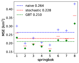
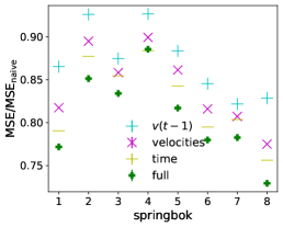
a) b) c)

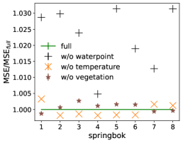
Figure 8: MSE of different forecasting models for individual springboks, which are distinguished by the numbers on the axis. (a) Comparison of the basic model, the stochastic AR(1) model, and the GBT-based model using all features. (b) Comparison of the mean squared error, normalized by the prediction of the basic model for GBT-models with information of the last step $v(t-1)$, movements on the last day (velocities), movements on the last day and time of the year (time), and all available information (full). (c) Comparison of the error normalized by the error of the full model versus the models where one of the features was removed. Note that in cases when no vertical lines are visible, the corresponding error is negligibly small.

Model	MSE $[\mathrm{km}^{2}/\mathrm{h}^{2}]$	MSE/MSEbasic	MSE/MSEfull
basic	0.264	1.0	1.257
AR(1)	0.228	0.873	1.087
AR(2)	0.228	0.873	1.087
$v_{t-1}$	0.228	0.872	1.082
velocities	0.219	0.841	1.044
time	0.215	0.825	1.023
full	0.210	0.795	1.0

Table 1: Mean squared error and relative error for different models of springbok movement. The values are averages over all individuals in the dataset. As seen from the third column the full model established here reduces the error in springbok move prediction by around 20%, as compared to the basic model.

As we are interested in forecasting the movement to be made by a springbok in the next hour ($\Delta t=1$ h), encoded by the "velocity" (distance per unit time of 1 h)

$$\mathbf{v}(t_{i})=\frac{\mathbf{r}(t_{i})-\mathbf{r}(t_{i-1})}{\Delta t},$$ (18)

the simplest prediction is to assume that, most probably, the next position is equal the current position. Then the predicted velocity $\tilde{\mathbf{v}}(t_{i})$ vanishes, i.e., $\tilde{\mathbf{v}}(t_{i})=0$. Viewing $\mathbf{v}$ as an averaged quantity, this simplified assumption corresponds to the picture of Brownian motion, in which steps in either direction are equally probable, and, as already noted by Pearson pearson1 , the next displacement is zero. How realistic this simple prediction or similar ones are can be quantified in terms of the mean squared error (MSE), evaluated as squared deviation of the forecast $\tilde{\mathbf{v}}$ with respect to the actual experimental time series $\mathbf{v}$,

$$\mathrm{MSE}=\frac{1}{L-1}\sum_{i=1}^{L-1}\left(\mathbf{v}(t_{i})-\tilde{\mathbf{v}}(t_{i})\right)^{2}.$$ (19)

MSEs, or normalized MSEs when compared to a given model, are common measures for the quality of models in modeling analyses, see, e.g., henrik ; munoz2021objective .

A better prediction is expected if the information contained in model (8) is taken into account. For short lag times of around one hour, confinement effects can be neglected, as these enter only with a comparatively long correlation time $\tau_{l}$, which is on the order of tens of hours, according to Fig. 4. The resulting model is then a random walk with correlated increments, characterized by the correlation time $\tau_{s}$. Thus, at such short lag times the prediction is given by

$$\mathbf{v}(t_{i})=e^{-\Delta t/\tau_{s}}\mathbf{v}(t_{i-1}),$$ (20)

in which each component corresponds to an autoregressive model of order one, AR(1). It can be tested that the full AR(2) model (8) does not lead to any significant improvement of the predictions (see table 1). In fact, model (20) already represents a significant improvement as compared to the naive Brownian prediction and explains around 13% of the squared error (see table 1).

V.2 Machine-learning approach

However, as mentioned above, model (20) is still quite simplistic and neither takes into account the specific animal movements at certain times of the day or year nor the position of the water points, the dependence on explorations during the previous day, as well as other factors (such as variable levels of vegetation or fluctuating temperatures). Obviously, a general model that could take such features into account is hard to formulate explicitly. Therefore it is useful to look for suitable machine learning algorithms. These methods karn19rnn-dl are superior to many classical techniques for model selection for the datasets generated from stochastic processes thapa ; fabr18 ; munoz2021objective ; aliv21dl-pnas ; henrik . They can also be used to infer the dynamical changes and the transition points song2022machine . A direct forecast of future steps of an animal using ML is less common in studying diffusion and foraging (for a review of potential methods we refer the reader to Ref. Dormann18 ), but it is already wide-spread in other disciplines such as power-grid frequency KRUSE2021100365 or air-pollution research cabaneros2019review . In these disciplines, the question "how important is the individual feature for the accuracy of modeling" is often being discussed. The same techniques can be applied for time-series analysis of animal movement. We deploy a supervised-ML model, which takes the following features into account:

• $\mathbf{v}(t_{i-1})$, the distance per time covered by an animal in the last hour (i.e., for a lag time $\Delta t=1$ h)

• $\mathbf{v}(t_{i-2})$, the distance per time covered in the hour before that

• $\mathbf{v}(t_{i-24})$, the distance per time walked in the same hour of the previous day

• $\mathbf{r}(t_{i-1})-\mathbf{r}(t_{i-24})$, the overall distance directions traveled in the last 24 hours

• $w(t_{i-1})$, the distance to the closest water point, and $w(t_{i-1})-w(t_{i-2})$, the change in distance from the closest water point during the last hour

• $T(\mathbf{r}(t_{i-1}))$, the temperature at the current position

• $V(\mathbf{r}(t_{i-1}))$, the vegetation type as a "lushness coefficient" (varying in the interval $[0,1]$) at the current position, and the lushness difference $V(\mathbf{r}(t_{i-1}))-V(\mathbf{r}(t_{i-2}))$ as compared to the previous location.

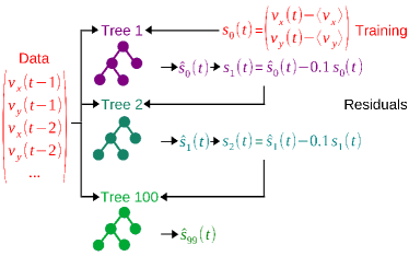
Figure 9: Schematic diagram of the GBT-algorithm: the first tree receives as input the residuals $s_{0}$ of the inputs and the average result of the training set. Depending on the specific input values, the tree’s output, the estimator $\hat{s}_{0}$ can take different values (one of the branches of the tree), which are trained from the results in the training set $(v_{x}(t),v_{y}(t))$, that ended up on the same branch of the tree. The output is regularized by the learning rate $0.1$. The residuals $s_{1}$ are passed as an input to the next tree, which works in the same way. The maximum number of trees in our application was 100. After the model is trained the output can be calculated from a new input as $(\hat{v}_{x}(t),\hat{v}_{y}(t))=(\langle v_{x}\rangle,\langle v_{y}\rangle)+0.1(\hat{s}_{0}(t)+\hat{s}_{1}(t)+\ldots+\hat{s}_{99}(t))$, where $(\langle v_{x}\rangle,\langle v_{y}\rangle)$ are the mean displacements in the training set.

Gradient-boosted trees (GBTs) represent a popular tool for regression analyses GBTfriedman ; GBTnatekin . GBTs are based on simple decision trees, and the output of one tree is then passed to the next decision tree, which learns how the residuals can be improved with additional questions. The result of each tree is regularized by a factor, called the learning rate. Choosing a sufficiently small learning rate reduces the risk of over-fitting KRUSE2021100365 . We use a learning rate of $0.1$, which is a standard choice for gradient-boosting machines. The number of trees and the maximal depth of the trees are the parameters to be chosen prior to starting the algorithm. We use $n=100$ trees with a maximal depth of 5, which was decided after comparing the accuracy of the algorithm for different sets of parameters. We employ the Python scikit-learn library for a supervised ML-model implemented as GBTs. The black-box character of such a model could be understood via running the model with different features acting as inputs and comparing the importance of each feature, see below. We note that in this GBT approach we do not use any specific information regarding the physical position of the springboks, but only account for their relative distances. The algorithm is thus applicable to all springboks independently of whether or not the area has already been explored previously. The data on vegetation levels and the data on temperature variations are taken from heringdon .

In Fig. 8 we compare the MSE of the basic (Brownian) model, the prediction from the AR(1) model (20), and the supervised ML-model. For the latter two, the models were trained on all but one individual and the next step was predicted for this remaining individual. In the case of the stochastic model, only the parameter $\tau_{s}$ had to be "learned": it can be obtained from minimizing $[\mathbf{v}(t_{i})-e^{-(1h)/\tau_{s}}\mathbf{v}(t_{i-1})]^{2}$. The stochastic model reduces the MSE of the prediction by $\approx$13% on average. Using all available features in the GBT model leads to a total reduction the MSE of $\approx$20%, see the entry 0.795 in the third column of Tab. 1. Consequently, the springbok motion contains a significant degree of stochasticity that cannot be explained even with the quite broad features of the GBT approach. We also mention the measurable variability of the MSE-results computed for movements of different individuals in Fig. 8, resulting from characteristics like age, size, gender, distinct set of explored terrain patterns, movement strategy (residential vs. migrating), etc..

V.3 Feature gain

ML-models such as GBTs can be considered as "black boxes": the effects of an individual feature are not immediately obvious. The easiest way to gain some insight into such a black box is to run the algorithm repeatedly and to examine the effects of adding or deleting certain individual features. More information should lead to a better prediction of the future behavior, but the question is how relevant an individual feature is for such predictions.

In Fig. 8b we demonstrate how subsequently adding information reduces the MSE. Errors are normalized by the error of the basic model (the variance of the velocity). It can be shown that taking into account only the previous data point—i.e., the same amount of information considered for the stochastic forecast—very well reproduces the MSE of the stochastic model, $\approx$13% (see Table 1). Adding information about the springbok paths during the previous hour and on the previous day, $\mathbf{v}(t_{i-2})$, $\mathbf{v}(t_{i-24})$, $\mathbf{r}(t_{i-1})-\mathbf{r}(t_{i-24})$ as three additional features yields a strong improvement of the error: it is almost 16% better than the basic model. Also, taking into account the time of the day and and of the year gives rise to another visible improvement, as can be expected from the changes of the dynamics depending on time discussed above. The information on changes in the distance to the water points has some effect, while the vegetation level, and the actual temperature lead to hardly any additional improvement. One reason might be, that some of this information is already included in the movement on the previous day, e.g. if the animal already visited the same water point or went to the same pasture to eat.

Looking at these three factors (previous data point, longer movement history, time of day/year) in detail, we can also consider the relative increase of the MSE upon removal of either features from the full model, as shown in Fig. 8c. We see that there is only one of the three factors that has a negative effect throughout all individuals, namely, the distance from the water points. The magnitude of the effect is, however, rather small. It is not clear that the model benefits much from information on the vegetation and temperature. For the vegetation, this is not an expected result, however, in order to predict where the animal goes to eat one would need more information about the surroundings and a higher temporal and spacial resolution.

VI Conclusion

We studied the movement dynamics of an ensemble of springboks, whose positions were recorded by long-term GPS tracking. Our analysis combines new statistical observables with stochastic models and ML-based feature analysis. Although the studied springbok ensemble is relatively small and the statistical quality of our results is therefore limited, we believe that this study will be a solid basis for more elaborate experimental field work and extraction of dynamic features from the garnered data. In particular, all techniques discussed here should be easily adaptable to the analysis of the movement dynamics of other ruminants. With sufficient modifications, possibly including the underlying stochastic models, the movement dynamics of other tracked animal species can be approached with the same methodology. In this sense our analysis presents a next step from the purely statistical description of animal movements, in the direction of a more detailed, biologically-inspired analysis and prediction.

The evaluation of the model performance ("forecasting error") for the movement in the following hour was based on the MSE obtained from comparison of the predicted movement of a given animal based on the model (after training of the model parameters from all other individuals) with actual animal movement. A simple model chosen for the movement dynamics was the discrete OU-process with correlated driving, corresponding to the autoregressive model AR(2). This process includes the confinement of the animal motion over time ranges of some $10^{2}$ h corresponding to a few km, as seen from the detailed TAMSD data. For the movement within the chosen 1 h lag time for the prediction analysis, the AR(2) model reduces to the AR(1) process, an unconfined, correlated motion. This model was shown to already have a quite good forecasting power, leading to a reduction of the MSE as compared to a basic model, in which animals on average stay put at their current positions. The gain in prediction from the correlated motion model was $\approx 13\%$. The error did not vary appreciably between this AR(1) model, the full AR(2) model, and even the GBT model, when the latter was solely trained on the previous position.

Naturally, a homogeneous model such as AR(1) with two parameters (diffusivity or noise strength and correlation time $\tau_{s}$) misses many relevant features of the real animal movement dynamics. A prime feature here is the daily cycle in the animal behavior. Using a decomposition technique based on the scaling exponents of total displacement, activity, and directedness, shows that not only the activity, but also the directedness of the springbok motion is higher during the day (the corresponding exponent is $\approx 1.5$) than during the night (with exponent $\approx 1.3$).

Taking into account the step at the same hour on the previous day, the daily displacement, and the last two steps, the error of the prediction is reduced by $\approx 16\%$ as compared to the basic model, as some of the daily dynamics is captured. The prediction is even better when information about the time of the year is added as well, because there is a difference between the behavior during wet versus dry seasons. A model with information about the time of day and of the year improves the naive prediction with the basic model by $\approx 18\%$. Note that such models do not have any specific information about the underlying map and are thus purely dynamical formulations. An important feature of the concrete physical landscape were shown to be the water points. While the scatter of the visited water points is higher than that of the resting points, the information of the water point distances turned out to have a clear effect. In contrast, including the current temperature did not improve the model prediction, similar to the lushness and its gradient. However, it is not immediately clear to which extent the information about temperature bears on the movement dynamics at all. Moreover, it would be reasonable to assume that the geographic abundance of food is encoded in the movements themselves. For an improved model, one could consider the food landscape in the entire field of vision of the animals and their memory.

Our best ML-based model with all information improved the MSE by about 20%. While this points at the relevance of the underlying parameters it also shows the limitation of the predictability, pointing at a good degree of stochasticity of individual motion. We propose that the reasons for this are not only the heterogeneity among the individuals reflected in variability of their movement parameters, but also in the multiple decisions taken in dependence of the current needs of an individual and its interactions with other animals, as well as personal perceptions. Averaging over different individuals from different herds leads to a loss of details of the individual animal movement. Concurrently, such averaging unveils features such as the motion directedness during day and night, scattering of water points and resting positions, and the predictability of the springbok movement without any knowledge of the underlying landscape. When more detailed data will be available, we will be able to extend our analysis on exact geographical features such as detailed vegetation and height maps, as well as the positions of fences and of other animals in the herd. In such an analysis also the time resolution of water availability at water points can be taken into consideration. However, it is an open questions whether such details are actually that important, or whether it is sufficient to have knowledge about more generic motion patterns.

We conclude by speculating that a substantial improvement of the relatively simple, few-parameter approaches outlined here, in combination with machine learning, may still be achievable. Namely, from feature-based machine learning studies we know that few additional features, on top of a substantial number already used, may significantly improve the predictions. Here AI combining all available information may be used in the future to pinpoint additional relevant factors in movement ecology.

Appendix A A primer on the Mandelbrot decomposition method

The central limit theorem for the sum of random variables guarantees the convergence to a Gaussian PDF if these random variables are independent, identically distributed, and of finite variance hughes . Violation of any of these conditions effects changes to the resulting PDF. When a diffusive process deviates from the Gaussian statistic of normal Brownian motion, a direct test of which of these conditions is violated, can be based on three scaling exponents defined on the basis of the increments of the position time series mand68moses ; che17 ; meyer18 ; aghion2021moses ; vilk .

Consider the position time-series $\mathbf{r}(t)$ as function of time $t$, described by the discrete sum of random increments $\mathbf{r}(N\Delta t)=\sum_{j=1}^{N}\delta\mathbf{r}_{j}$, where $\delta\mathbf{r}_{j}\equiv\mathbf{r}(j\Delta t)-\mathbf{r}([j-1]\Delta t)$ and $N=t/\Delta t$, and $0<\Delta t\ll t$ is an arbitrary time increment. We also define the average velocity vector in the $j$th increment, $\mathbf{v}_{j}\equiv\delta\mathbf{r}_{j}/\Delta t$. From these quantities we calculate the scaling of three observables: (i) the mean absolute velocity $\langle|\mathbf{v}|\rangle$, (ii) the mean squared velocity $\langle\mathbf{v}^{2}\rangle$, and (iii) the ensemble-averaged time-averaged MSD (TAMSD). These are connected to the following effects:

(i) Non-stationarity. The conditions that the random variables are identically distributed is violated. Non-stationarity of the increments can be measured by the the "Moses" exponent $M$ defined in terms of

$$\left<\overline{|\mathbf{v}|(N\Delta t)}\right>=\left<\frac{1}{N\Delta t-\Delta t}\sum_{j=1}^{N}|\mathbf{v}_{j}|\right>\propto N^{M-1/2},$$ (21)

where the overline indicates time averaging (TA). When $M=1/2$ the increments are stationary and thus identically distributed. When $M>1/2$ the process is

(ii) Diverging variance. Extreme events in the time series are picked up by the "Noah" exponent $L$ (generally, $L\geq 1/2$ mand68moses ), given through

$$\left<\overline{\mathbf{v}^{2}(N\Delta t)}\right>\equiv\left<\frac{1}{N\Delta t-\Delta t}\sum_{j=1}^{N}\mathbf{v}^{2}_{j}\right>\propto N^{2L+2M-2}.$$ (22)

If in addition to $M=1/2$ we have $L=1/2$, then $\langle\mathbf{v}^{2}\rangle$ is constant. Yet, if $L>1/2$, its value will grow in time, even though $M=1/2$. While $\langle|\mathbf{v}|\rangle$ is a measure for the typical fluctuations in a time series, the quantity $\langle\mathbf{v}^{2}\rangle$ is sensitive to the tails of the velocity PDF. In absence of extreme events $\langle\mathbf{v}^{2}\rangle\propto N^{2M-1}$, thus $L\neq 1/2$ is an indicator for the occurrence of extreme events.

(iii) Temporal correlations. The "Joseph" exponent measures whether the increments of the process are independent or not. This exponent can be extracted from the scaling of the integrated velocity autocorrelation function

$$\frac{1}{\langle\mathbf{v}^{2}\rangle}\sum_{i=1}^{l}\langle\mathbf{v}_{i}\cdot\mathbf{v}_{i+l}\rangle\propto l^{2J-1}.$$ (23)

As this function is sometimes difficult to calculate from finite time series, an alternative definition is based on the mean time-averaged MSD

$$\left<\frac{1}{N-l}\sum_{i=1}^{N-l}\left(\mathbf{r}(t_{i+l})-\mathbf{r}(t_{i})\right)^{2}\right>\propto N^{2L+2M-2}l^{2J}.$$ (24)

For long-ranged temporal correlations (decaying very slowly in time) one has $J\neq 1/2$, thus violating the independence condition of the central limit theorem.

There exists a fundamental summation relation between $M$, $L$, $J$ and the Hurst exponent $H$ che17 ; meyer18 ; aghion2021moses ,

$$H=J+L+M-1.$$ (25)

This relation was empirically confirmed in a wide range of systems vilk . An observed process resembles Brownian motion when $L=M=J=H=1/2$. As we do not observe a growing variance $\langle\mathbf{v}^{2}\rangle$, and thus we assume $L=1/2$ in the main text.

The summation relation (25) for $L=1/2$ can be derived as follows. Assuming a power-law scaling dependence of the autocorrelation function with the lag time $\Delta$ and the measurement time $t$, we have (for the $x$-component)

$$\langle(x(t)-x(0))^{2}\rangle = 2\int_{0}^{t}d\Delta\int_{0}^{t-\Delta}dt^{\prime}\langle v(t^{\prime})v(t^{\prime}+\Delta)\rangle$$ (26)

$$\propto 2\int_{0}^{t}d\Delta\int_{0}^{t-\Delta}dt^{\prime}\langle v^{2}(t^{\prime})\rangle\Delta^{2J-2}$$

$$\propto 2\int_{0}^{t}d\Delta\Delta^{2J-2}\int_{0}^{t-\Delta}dt^{\prime}{t^{\prime}}^{2M-1}$$

$$\propto \frac{B(2J-1,2M+1)}{M}t^{2M+2J-1},$$

where the Euler Beta-function is given by

$$B(\alpha,\beta)=\int_{0}^{1}t^{\alpha-1}(1-t)^{\beta-1}dt.$$ (27)

The last step requires, that $J>1/2$ and $M>0$, which is true in our situation. In this case, relation (26) holds for all $t$ and $\Delta$, for smaller exponents it only holds in the long-time limit.

Competing interests

The authors have no competing interests to declare.

Data availability

The data-set is available upon reasonable request from the authors.

References

- (1) R. Ross, Science 22, 689 (1905).
- (2) K. Pearson, Nature 72, 294 (1905).
- (3) Lord Rayleigh, Nature 72, 318 (1905).
- (4) K. Pearson, Nature 72, 342 (1905).
- (5) B. D. Hughes, Random walks and random environments, vol 1: random walks (Oxford University Press, Oxford, UK, 1995).
- (6) E. A. Codling, M. J. Plank, and S. Benhamou, J. Roy. Soc. Interface 5, 813 (2008).
- (7) A. Einstein, Ann. Phys. (Leipzig) 322, 549 (1905).
- (8) M. von Smoluchowski, Ann. Phys. (Leipzig) 21, 756 (1906).
- (9) E. Benson, Wired wilderness: Technologies of tracking and the making of modern wildlife (Johns Hopkins University Press, Baltimore MY, 2010).
- (10) F. Cagnacci, L. Boitani, R. A. Powell, and M. S. Boyce, Phil. Trans. Roy. Soc. B 365, 2157 (2010).
- (11) M. Holyoak, R. Casagrandi, R. Nathan, E. Revilla, and O. Spiegel, Proc. Natl. Acad. Sci. USA 105, 19060 (2008).
- (12) M. J. E. Broekman, J. P. Hilbers, M. A. J. Huijbregts, T. Mueller, A. H. Ali, H. Andren, J. Altmann, M. Aronsson, N. Attias, H. L. A. Bartlam-Brooks, et al., Glob. Ecol. Biogeog. 31, 1526 (2022).
- (13) S. Toledo, D. Shohami, I. Schiffner, E. Lourie, Y. Orchan, Y. Bartan, and R. Nathan, Science 369, 188 (2020).
- (14) C. E. Beardsworth, E. Gobbens, F. van Maarseveen, B. Denissen, A. Dekinga, R. Nathan, S. Toledo, and A. I. Bijleveld, Meth. Ecol. Evol. 13, 1990 (2022).
- (15) R. Nathan, W. M. Getz, E. Revilla, M. Holyoak, R. Kadmon, D. Saltz, and P. E. Smouse, Proc. Natl. Acad. Sci. USA 105, 19052 (2008).
- (16) R. Nathan, C. T. Monk, R. Arlinghaus, T. Adam, J. Alós, M. Assaf, H. Baktoft, C. E. Beardsworth, M. G. Bertram, A. I. Bijleveld, et al., Science 375, eabg1780 (2022).
- (17) K. Pearson and J. Blakeman, III. Mathematical contributions to the theory of evolution. XV.(Drapers’ company research memoirs. Biometric Series; London, Dulau and co, 1906).
- (18) J. G. Skellam, Biometrika 38, 196 (1951).
- (19) J. Brownlee, Proc. Roy. Soc. Edin. 31, 262 (1912).
- (20) M. A. Tucker, K. Boöhning-Gaese, W. F. Fagan, J. M. Fryxell, B. V. Moorter, S. C. Alberts, A. H. Ali, A. M. Allen, N. Attias, T. Avgar, et al., Science 359, 466 (2018).
- (21) O. Vilk, Y. Orchan, M. Charter, N. Ganot, S. Toledo, R. Nathan, and M. Assaf, Phys. Rev. X 12, 031005 (2022).
- (22) S. Rotics, M. Kaatz, Y. S. Resheff, S. F. Turjeman, D. Zurell, N. Sapir, U. Eggers, A. Flack, W. Fiedler, F. Jeltsch, et al., J. Anim. Ecol. 85, 938 (2016).
- (23) O. Vilk, E. Aghion, T. Avgar, C. Beta, O. Nagel, A. Sabri, R. Sarfati, D. K. Schwartz, M. Weiss, D. Krapf, R. Nathan, R. Metzler, and M. Assaf, Phys. Rev. Res. 4, 033055 (2022).
- (24) M. Roeleke, U. E. Schlägel, C. Gallagher, J. Pufelski, T. Blohm, R. Nathan, S. Toledo, F. Jeltsch, and C. C. Voigt, Proc. Natl. Acad. Sci. USA 119, e2203663119 (2022).
- (25) D. W. Sims, E. J. Southall, N. E. Humphries, G. C. Hays, C. J. Bradshaw, J. W. Pitchford, A. James, M. Z. Ahmed, A. S. Brierley, M. A. Hindell, et al., Nature 451, 1098 (2008).
- (26) D. W. Sims, N. E. Humphries, R. W. Bradford, and B. D. Bruce, J. Anim. Ecol. 81, 432 (2011).
- (27) E. Gurarie, C. Bracis, M. Delgado, T. D. Meckley, I. Kojola, and C. M. Wagner, J. Anim. Ecol. 85, 69 (2016).
- (28) R. Fürth, Zeit. f. Phys. 2, 244 (1920).
- (29) P. M. Kareiva and N. Shigesada, Oecolog. 56, 234 (1983).
- (30) F. Bartumeus, M. G. E. da Luz, G. M. Viswanathan, and J. Catalan, Ecol. 86, 3078 (2005).
- (31) P. Romanczuk, M. Bär, W. Ebeling, B. Lindner, and L. Schimansky-Geier, Euro. Phys. J. Spec. Top. 202, 1 (2012).
- (32) E. Lemaitre, I. M. Sokolov, R. Metzler, and A. V. Chechkin, New J. Phys. 25, 013010 (2023).
- (33) E. Gurarie, C. H. Fleming, W. F. Fagan, K. L. Laidre, J. Hernández-Pliego, and O. Ovaskainen, Mov. Ecol. 5, 13 (2017).
- (34) B. B. Mandelbrot and J. W. van Ness, SIAM Rev. 10, 422 (1968).
- (35) R. Metzler and J. Klafter, Phys. Rep. 339, 1 (2000).
- (36) R. Metzler, J.-H. Jeon, A. G. Cherstvy, and E. Barkai, Phys. Chem. Chem. Phys. 16, 24128 (2014).
- (37) Y. Meroz and I. M. Sokolov, Phys. Rep. 573, 1 (2015).
- (38) D. Molina-Garcia, T. Sandev, H. Safdari, G. Pagnini, A. Chechkin, and R. Metzler, New J. Phys. 20, 103027 (2018).
- (39) T. Guggenberger, A. V. Chechkin, and R. Metzler, New J. Phys. 24, 073006 (2022).
- (40) M. Dahlenburg, A. V. Chechkin, R. Schumer, and R. Metzler, Phys. Rev. E 103, 052123 (2021).
- (41) O. Tal-Friedman, Y. Roichman, and S. Reuveni, Phys. Rev. E 106, 054116 (2022).
- (42) M. R. Evans and S. N. Majumdar, Phys. Rev. Lett. 106, 160601 (2011).
- (43) M. R. Evans, S. N. Majumdar, and G. Schehr, J. Phys. A 53, 193001 (2020).
- (44) I. Abdoli and A. Sharma, Soft Matt. 17, 1307 (2021).
- (45) A. S. Bodrova, A. V. Chechkin, and I. M. Sokolov, Phys. Rev. E 100, 012119 (2019).
- (46) P. Xu, T. Zhou, R. Metzler, and W. Deng, New J. Phys. 24, 033003 (2022).
- (47) V. Stojkoski, P. Jolakoski, A. Pal, T. Sandev, L. Kocarev, and R. Metzler, Philos. Trans. A 380, 20210157 (2022).
- (48) K. Zelenkovski, T. Sandev, R. Metzler, L. Kocarev, and L. Basnarkov, Entropy 25, 293 (2023).
- (49) W. Wang, A. Cherstvy, H. Kantz, R. Metzler, and I. Sokolov, Phys. Rev. E 104, 024105 (2021).
- (50) W. Wang, A. Cherstvy, R. Metzler, and I. Sokolov, Phys. Rev. Res. 4, 013161 (2022).
- (51) A. V. Chechkin and I. M. Sokolov, Phys. Rev. Lett. 121, 050601 (2018).
- (52) I. M. Sokolov, Phys. Rev. Lett. 130, 067101 (2023).
- (53) O. Bénichou, C. Loverdo, M. Moreau, and R. Voituriez, Rev. Mod. Phys. 83, 81 (2011).
- (54) P. C. Bressloff and J. M. Newby, Rev. Mod. Phys. 85, 135 (2013).
- (55) O. Bénichou, M. Coppey, M. Moreau, P. H. Suet, and R. Voituriez Phys. Rev. Lett. 94, 198101 (2005).
- (56) O. Bénichou, C. Loverdo, M. Moreau, and R. Voituriez, Phys. Rev. E 74, 020102 (2006).
- (57) G. M. Viswanathan, M. G. E. Da Luz, E. P. Raposo, and H. E. Stanley, The physics of foraging: an introduction to random searches and biological encounters (Cambridge University Press, Cambridge UK, 2011).
- (58) M. A. Lomholt, T. Koren, R. Metzler, and J. Klafter, Proc. Natl. Acad. Sci. USA 105, 11055 (2008).
- (59) V. Palyulin, A. V. Chechkin, R. Klages, and R. Metzler, J. Phys. A 49, 394002 (2016).
- (60) B. B. Mandelbrot, The fractal geometry of nature (W. H. Freeman, New York, NY, 1982).
- (61) M. F. Shlesinger and J. Klafter, in On growth and form, edited by H. E. Stanley and N. Ostrowsky (Martinus Neijhoff, Dordrecht, The Netherlands, 1986).
- (62) M. A. Lomholt, T. Ambjörnsson, and R. Metzler, Phys. Rev. Lett. 95, 260603 (2005).
- (63) G. M. Viswanathan, V. Afanasyev, S. V. Buldyrev, E. J. Murphy, P. A. Prince, and H. E. Stanley, Nature 381, 413 (1996).
- (64) G. M. Viswanathan, S. V. Buldyrev, S. Havlin, M. G. E. da Luz, E. P. Raposo, and H. E. Stanley, Nature 401, 911 (1999).
- (65) A. M. Edwards, R. A. Phillips, N. W. Watkins, M. P. Freeman, E. J. Murphy, V. Afanasyev, S. V. Buldyrev, M. G. da Luz, E. P. Raposo, H. E. Stanley, et al., Nature 449, 1044 (2007).
- (66) N. E. Humphries, H. Weimerskirch, N. Queiroz, E. J. Southall, and D. W. Sims, Proc. Natl. Acad. Sci. USA 109, 7169 (2012).
- (67) E. Gurarie, R. D. Andrews, and K. L. Laidre, Ecol. Lett. 12, 395 (2009).
- (68) E. Gurarie, C. Bracis, A. Brilliantova, I. Kojola, J. Suutarinen, O. Ovaskainen, S. Potluri, and W. F. Fagan, Front. Ecol. Evol. 10, 768478 (2022).
- (69) D. Boyer, G. Ramos-Fernandez, O. Miramontes, J. L. Mateos, G. Cocho, H. Larralde, H. Ramos, and F. Rojas, Proc. Roy. Soc. B 273, 1743 (2006).
- (70) D. Boyer and C. Solis-Salas, Phys. Rev. Lett. 112, 240601 (2014).
- (71) N. E. Humphries, N. Queiroz, J. R. M. Dyer, N. G. Pade, M. K. Musyl, K. M. Schaefer, D. W. Fuller, J. M. Brunnschweiler, T. K. Doyle, J. D. R. Houghton, et al., Nature 465, 1066 (2010).
- (72) G. M. Viswanathan, Nature 465, 1018 (2010).
- (73) M. de Jager, F. J. Weissing, P. M. J. Herman, B. A. Nolet, A and J. van de Koppel, Math. Theory Sci. Rand. Migrat. 332, 1551 (2011).
- (74) A. Reynolds, G. Santini, G. Chelazzi, and S. Focardi, Roy. Soc. Open Sci. 4, 160941 (2017).
- (75) J. F. Terlau, U. Brose, B. Thomas, P. Samraat, M. Pinsky, and M. R. Hirt, DOI: 10.21203/rs.3.rs-2333180/v1 (2022).
- (76) T. Shokaku, T. Moriyama, H. Murakami, S. Shinohara, N. Manome, and K. Morioka, Review of Sci. Instr. 91, 104104 (2020).
- (77) D. A. Raichlen, B. M. Wood, A. D. Gordon, A. Z. P. Mabulla, F. W. Marlowe, and H. Pontzer, Proc. Natl. Acad. Sci. 111, 728 (2014).
- (78) D. Brockmann, L. Hufnagel, and T. Geisel, Nature 439, 462 (2006).
- (79) P. Wang, A.-L. Barabási, C. Song, and T. Koren, Nature Phys. 6, 818 (2010).
- (80) B. Gross, Z. Zheng, S. Liu, X. Chen, A. Sela, J. Li, D. Li, and S. Havlin, Europhys. Lett. 131, 58003 (2020).
- (81) V. V. Palyulin, A. V. Chechkin, and R. Metzler, Proc. Natl. Acad. Sci. USA 111, 2931 (2014).
- (82) G. H. Pyke, Meth. Ecol. Evol. 6, 1 (2015).
- (83) J. Travis, Science 318, 742 (2007).
- (84) A. M. Edwards, M. P. Freeman, G. A. Breed, and I. D. Jonsen, PLoS ONE 7, 1 (2012).
- (85) W. F. Fagan, M. A. Lewis, M. Auger-Methe, T. Avgar, S. Benhamou, G. Breed, L. LaDage, U. E. Schlagel, W.-W. Tang, Y. P. Papastamatiou, et al., Ecol. Lett. 16, 1316 (2013).
- (86) M. Panzacchi, B. Van Moorter, O. Strand, M. Saerens, I. Kivimäki, C. C. St. Clair, I. Herfindal, and L. Boitani, J. Anim. Ecol. 85, 32 (2016).
- (87) R. Chen, O. Spiegel, Y. Bartan, and R. Nathan, Anim. Behav. 191, 15 (2022).
- (88) U. E. Schlägel, V. Grimm, N. Blaum, P. Colangeli, M. Dammhahn, J. A. Eccard, S. L. Hausmann, A. Herde, H. Hofer, J. Joshi, et al., Biol. Rev. 95, 1073 (2020).
- (89) J. R. Potts and U. E. Schlägel, Meth. Ecol. Evol. 11, 1092 (2020).
- (90) S. Benhamou, J. Theor. Biol. 229, 209 (2004).
- (91) F. Walther, Verhalten der Gazellen (A. Ziemsen Verlag, Wittenberg, 1968).
- (92) R. C. Bigalke, Zoolog. Afric. 5, 59 (1970).
- (93) R. Bigalke, Afric.Zool. 7, 333 (1972).
- (94) J. H. M. David, Zoolog. Afric 13, 115 (1978).
- (95) G. Skinner, Transvaal Museum Monog. 10, 19 (1996).
- (96) R. Hering, M. Hauptfleisch, M. Jago, T. Smith, S. Kramer-Schadt, J. Stiegler, and N. Blaum, Front. Ecol. Evol. 10, 907079 (2022).
- (97) R. Hering, M. Hauptfleisch, M. Jago, T. Smith, S. Kramer-Schadt, J. Stiegler, and N. Blaum, Front. Ecol. Evol. 10, 90707 (2022).
- (98) P. Bovet and S. Benhamou, J. Theor. Biol. 131, 419 (1988).
- (99) U. Bhat and S. Redner, J. Stat. Mech. 2022, 033402 (2022).
- (100) D. Krapf, N. Lukat, E. Marinari, R. Metzler, G. Oshanin, C. Selhuber-Unkel, A. Squarcini, L. Stadler, M. Weiss, and X. Xu, Phys. Rev. X 9, 011019 (2019).
- (101) O. Vilk, E. Aghion, R. Nathan, S. Toledo, R. Metzler, and M. Assaf, J. Phys. A 55, 334004 (2022).
- (102) E. Barkai, Y. Garini, and R. Metzler, Phys. Today 65(8), 29 (2012).
- (103) S. Burov, R. Metzler, and E. Barkai, Proc. Natl. Acad. Sci. USA 107, 13228 (2010).
- (104) A. P. Ghosh, W. Qin, and A. Roitershtein, J. Interdisc. Math. 19, 1 (2016).
- (105) W. Qin, Discrete Ornstein-Uhlenbeck process in a stationary dynamic enviroment, PhD thesis, Iowa State University, 2011.
- (106) D. W-Ch. Miao, J. Appl. Prob. 50, 1102 (2013).
- (107) G. E. Box, G. M. Jenkins, G. C. Reinsel, and G. M. Ljung, Time series analysis: forecasting and control (J. Wiley & Sons, London, 2015).
- (108) L. S. Ornstein, Proc. Roy. Acad. Amst. 21, 96 (1917).
- (109) G. E. Uhlenbeck and L. S. Ornstein, Phys. Rev. 36, 823 (1930).
- (110) A. G. Cherstvy, S. Thapa, Y. Mardoukhi, A. V. Chechkin, and R. Metzler, Phys. Rev. E 98, 022134 (2018).
- (111) H. Risken, The Fokker-Planck equation (Springer, Heidelberg, 1989).
- (112) P. G. Meyer and R. Metzler (unpublished).
- (113) C. Bechinger, R. Di Leonardo, H. Löwen, C. Reichhardt, G. Volpe, and G. Volpe, Rev. Mod. Phys. 88, 045006 (2016).
- (114) S. Jespersen, R. Metzler, and H. C. Fogedby, Phys. Rev. E 59, 2736 (1999).
- (115) A. V. Chechkin, J. Klafter, V. Yu. Gonchar, R. Metzler, and L. V. Tanatarov, Phys. Rev. E 67, 010102(R) (2003).
- (116) A. V. Chechkin, V. Yu. Gonchar, J. Klafter, R. Metzler, and L. V. Tanatarov, J. Stat. Phys. 115, 1505 (2004).
- (117) K. Capała, A. Padash, A. V. Chechkin, B. Shokri, R. Metzler, and B. Dybiec, Chaos 30, 123103 (2020).
- (118) P. Xu, T. Zhou, R. Metzler, and W. Deng, Phys. Rev. E 101, 062127 (2020).
- (119) P. Xu, T. Zhou, R. Metzler, and W. Deng, New J. Phys. 24, 033003 (2022).
- (120) T. Guggenberger, G. Pagnini, T. Vojta, and R. Metzler, New J. Phys. 21, 022002 (2019).
- (121) T. Guggenberger, A. Chechkin, and R. Metzler, J. Phys. A 54, 29LT01 (2021).
- (122) C. Maggi, M. Paoluzzi, N. Pellicciotta, A. Lepore, L. Angelani, and R. Di Leonardo, Phys. Rev. Lett. 113, 238303 (2014).
- (123) E. Fodor, C. Nardini, M. E. Cates, J. Tailleur, P. Visco, and F. van Wijland, Phys. Rev. Lett. 117, 038103 (2016).
- (124) P. G. Meyer and H. Kantz, New J. Phys. 21, 033022 (2019).
- (125) J. W. CAIN III, P. R. Krausman, S. S. Rosenstock, and J. C. Turner, Wildlife Soc. Bull. 34, 570 (2006).
- (126) C. Roche, Africa 78, 157 (2008).
- (127) P. G. Meyer, V. Adlakha, H. Kantz, and K. E. Bassler, New J. Phys. 20, 113033 (2018).
- (128) E. Aghion, P. G. Meyer, V. Adlakha, H. Kantz, and K. E. Bassler, New J. Phys. 23, 023002 (2021).
- (129) P. G. Meyer, E. Aghion, and H. Kantz, J. Phys. A 55, 274001 (2022).
- (130) B. B. Mandelbrot and J. R. Wallis, Wat. Res. Res. 4, 909 (1968).
- (131) L. Chen, K. E. Bassler, J. L. McCauley, and G. H. Gu- naratne, Physical Review E 95, 042141 (2017).
- (132) E. Aghion, P. G. Meyer, V. Adlakha, H. Kantz, and K. E. Bassler, New J. Phys. 23, 023002 (2021).
- (133) B. T. McClintock and T. Michelot, Meth. Ecol. Evol. 9, 1518 (2018).
- (134) R. Patin, M.-P. Etienne, E. Lebarbier, S. Chamaillé-Jammes, and S. Benhamou, J. Anim. Ecol. 89, 44 (2020).
- (135) H. Seckler and R. Metzler, Nat. Commun. 13, 6717 (2022).
- (136) G. Muñoz-Gil, G. Volpe, M. A. Garcia-March, E. Aghion, A. Argun, C. B. Hong, T. Bland, S. Bo, J. A. Conejero, N. Firbas, et al., Nat. Commun. 12, 1 (2021).
- (137) M. Raissi, P. Perdikaris, and G. E. Karniadakis, J. Comp. Phys. 378, 686 (2019).
- (138) S. Thapa, M. A. Lomholt, J. Krog, A. G. Cherstvy, and R. Metzler, Phys. Chem. Chem. Phys. 20, 29018 (2018).
- (139) C. Mark, C. Metzner, L. Lautscham, P. L. Strissel, R. Strick, and B. Fabry, Nat. Commun. 9, 1803 (2018).
- (140) V. Jamali, C. Hargus, A. Ben-Moshe, A. Aghazadeh, H. D. Ha, K. K. Mandadapu, and A. P. Alivisatos, Proc. Natl. Acad. Sci. 118, e2017616118 (2021).
- (141) T. Song, Y. Choi, J.-H. Jeon, and Y.-K. Cho, bioRxiv DOI: 10.1101/2022.07.07.499070.
- (142) C. F. Dormann, J. M. Calabrese, G. Guillera-Arroita, E. Matechou, V. Bahn, K. Bartoń, C. M. Beale, S. Ciuti, J. Elith, K. Gerstner, et al., Ecological Monographs 88, 485 (2018).
- (143) J. Kruse, B. Schaäfer, and D. Witthaut, Patterns 2, 100365 (2021).
- (144) S. M. Cabaneros, J. K. Calautit, and B. R. Hughes, Envir. Model. & Software 119, 285 (2019).
- (145) J. H. Friedman, Ann. Stat. 29, 1189 (2001).
- (146) A. Natekin and A. Knoll, Front. Neurorob. 7, 21 (2013).
- (147) Supplementary Material