Predictive change point detection for heterogeneous data

Abstract

An unsupervised change point detection (CPD) framework assisted by a predictive machine learning model called ”Predict and Compare” is introduced which is able to detect change points online. The framework admits different predictive models for the required time series forecasting (Predict) step together with different statistical tests for deciding about the proximity of predicted and actual data (Compare step). Its performance for the Predict step being carried out by either an LSTM recursive neural network or an ARIMA linear time series model together with the CUSUM rule as Compare step method is shown in relation to other state-of-the-art online CPD routines. It shows to perform best (low average detect time) in the regime of a low number of false positive detections. The method’s strength lies in detecting structural changes in the presence of complicated underlying trend patterns. The framework is formulated in general terms, so as to allow reasonable comparison with other similarly structured CPD methods. The use case concerns tribological wear for which change points separating the run-in, steady-state, and divergent wear phases are detected.

1 Introduction

1.1 The problem and our approach

Change point detection (CPD) in time series classically refers to analysing the observed data in order to identify abrupt changes in the underlying latent probability distribution Lai_95 ; Wu_05 ; odile_2018 . A classical approach in this area is CUSUMpageContinuousInspectionSchemes1954a , which sequentially tracks a cumulative sum and flags a distribution change when the value exceeds a threshold determined by a sequential test wald . This has been shown to be optimal in the sense of smallest detection times under the given expected length between false positives for asymptotically large average in-control run-lengths lord_1977 , and exact (finite sample) optimality in a decision theoretic (mini-max) sense mous_2004 ; ritov ; aue . The number of fields in which this detector finds applications is large (e.g. medical Yang_Heart , micro-economical harrison_Demand , portfolio managerial manner_Copula ; see burgEvaluationChangePoint2020 for a review).

A major distinction between change point detection techniques is whether change points (CPs) are determined after a batch sample has been obtained (offline mode), or whether they are continuously updated each time a new sample point is added (online mode). The latter is setting the scene for sequential tests, and is therefore also often referred to as sequential change point detection (amin_2017, , p. 4)siegmund ). The majority of CPD methods are offline truong , as they have a wider range of applicability due to the additional range of data points available after each proposed change point (unknown post-change parameters (cao, , Chap. 1.1)). The availability of the entire data set is also useful for an increased power of the tests. On the other hand, several types of processes involving the monitoring of sensor values are inherently online and therefore do not allow the use of offline techniques (e.g. quality management in production hawkinsCumulativeSumCharts1998 ; lim ). In amin_2017 ), Sect. 4.2, it is recognized that each online CPD algorithm employs a sliding time-interval of a certain size within which the decision about the presence of a CP is made. Furthermore, the use of additional ’retrospective’ windows characteristically belong to several online CPD methods amin_2017 . Namely, they are those belonging to Bayesian modeling, Gaussian Process modeling, Several online CPD algorithms, however, just compare the data on the two sliding windows, instead of using a prediction. Comparison between different distributions, such as by the Mann-Whittney test have recently been employed for developing a particle filter method for Capacity Reaction Point detection ma_rul_2021 . While this method belongs to the offline circle of CP detectors, there is a continuous transition from completely offline (size is infinity) to completely online (size equals zero) algorithms, and applications of particle filters may also find use in online techniques for small (tolerable) sliding window sizes.

It is precisely the sequential tests wald ; siegmund such as CUSUM, and Exponentially Weighted Moving Average (EWMA) models which are exploited in applications (e.g., production process quality control (SQC, , Chap. 9)) and which allow a rigorous online change point monitoring (cao, , Chapter 1.4). As noted in (amin_2017, , p. 22), it is an ongoing challenge to define online CPD methods for non-stationary data.

One important generalization away from the step-like change points consists of gradually changing location parameters buecher ; vogt ; aueSteinbach , called gradual change points. Already in (woodallSTATISTICALDESIGNCUSUM1993, , Chap 1.5) it is also pointed out, however, that test results for linear changes as opposed to step anomalies are not easy to distinguish in practice. Nevertheless, modeling gradual changes by linear transitions can already improve the characteristic average run length estimates of the CUSUM process bissell . A much more general assumption of the departure from step-anomalies is to suppose that stationarity only exists locally, for which vogt have shown the advantages of a ’refined CUSUM rule’.

A further generalization consists of dropping the assumption of zero mean stationarity between the change points. In (aue, , Sec. 2.2) the possibility to assume, more generally, the validity of a linear regression model between two change points is exploited. An efficient model to include such linear trends between change points which also works in the online case is given by Break detection for Additive Season and Trend (BFAST) verbesselt_detecting_2010 . Another successful method for online CPD for non-stationary data is by using a Bayesian approach AdamsMacKay , as discussed in (burgEvaluationChangePoint2020, , Chapter C.1), which also allows non-linear trends between change points. The online changepoint detection (OCD) by Chen et al. chen_OCD_2022 is a very recent online detection method that uses aggregated likelihood test statistics for detection. Together with the classical CUSUM rule we choose these methods as our benchmark references because they cover a wide methodological scope. We note that further recent approaches challenging the intermediate stationarity condition include optimization cao , and other Bayesian methods agudelo ; wang , also admitting non-trivial intermediate trends.

In the light of these generalizations, we presently address the problem of change point detection with emphasis to:

1. defining an online change point detector,

2. searching for CPs belonging to gradual changes with few false positives,

3. allowing for the presence of trends between CPs.
   

’Trend’ is meant here to refer to any systematic varying-in-time changes of the mean or the variance of the process, i.e. deviations from stationarity. The key idea of our Predict and Compare (P&C)  is the ability of the detector to differentiate between changes recognizable by a predictive model to belong to a ’pattern of the time-series’, and changes that are not recognized as such and therefore termed change point. A predictive model we call any function taking finite sub-intervals of a time-series as input and giving a finite sequence of values as a predicted estimation of the following progression of the time series as its output.

It is particularly difficult to detect a genuine change point in the presence of an underlying trend following a complicated pattern. While linear, damped, or seasonal trends are among the classically detectable patterns in time series analysis (see e.g. verbesselt_detecting_2010 , (gardner85, , Sect. 2.3)) trends following a less obvious pattern which can only be detected by non-linear predictive models are mistaken as CPs by conventional CPD methods. This typically leads to a high false positive detection rate. P&C  detects CPs only if they don’t match predictions of the possibly complicated trends learned by a predictive model.

Transition between noisy (exponential) Run-in and (linear) Steady State increasing signal

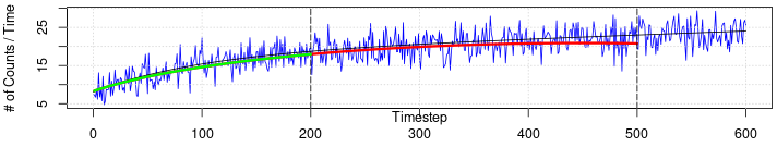
Figure 1: Principle of P&C: CP from a Run-in into a Steady-state regime (end of Sect. 1.1): At $t=200$, a forecast (red) with input window $\{1,\dots,200\}$ is shown. From the input data, only the dominant exponentially converging behavior is recognized. Therefore, only this ’damped’ behavior is extended in the forecast of the Predict step. The weak linear behavior of the steady-state wear -present throughout the data-set- eventually becomes dominant for growing time, but isn’t part of the prediction, which finally deviates from the raw data for $t\geq 350$ facilitating the CP-detection in the Compare step.

The technical implementation of this idea first involves a ’historic’ data set including the trend (abbrev. by $f$) from the ’distant past’ for training a model $\widehat{f}$ estimating $f$. The model $\widehat{f}$ takes a finite sequence as input data from a input window representing the immediate past before the current point in time and predicts the sequence of values on a time window immediately behind the current moment (called the prediction window). Thus, $\widehat{f}$ aims at capturing the general trend in the underlying probability distribution, so that significant (onsets of) changes from these predictions can be considered to be one of the CPs. Figure 1 shows this principle idea for the CP between an exponential run-in into a noisy linearly increasing process (Table 6 gives the results for comparable CPs on real tribological data).

The learning model involved in P&C  is trained to predict how the trend of the sequence of the time series progresses (Predict Step). For example, the run-in pattern typically observed after re-initiating a monitored production process is neither linear, nor periodic (see Figure 1). However, it is well predictable given only the onset of the run-in pattern from the input window. This is possible as long as it has been trained on a data set which includes sufficiently many run-in sub-processes of length fitting into the training window. The length of the training window thus restricts the recognizable pattern types to a certain maximal time scale. In P&C  the prediction estimate on the prediction window is then compared to the true data (Compare Step) to check for CPs present in addition to the predicted run-in pattern.

By heterogeneous data we mean that the distributions of the data between CPs may vary strongly. (cf. krause )). As long as $\widehat{f}$ has been trained to recognize any of the possible trend patterns they can occur as characteristics of the time series in between two CPs. Our approach belongs to the CPD methods which need a definition of ’normal data’ from which changes are recognized as CPs. What is normal in the case of P&C  is only defined by what the predictive model has been trained to recognize as such. As there is no need for labels, in this way, P&C  belongs to the unsupervised method types (see amin_2017 , Sect. 3.2). We note that the variations between the distributions before and after the CP may include trends- the processes between two CPs need not be stationary.

The paper starts in with stating scene-setting definitions of method and data in the beginning of Chapter 2. Then, after introducing the reference approaches, we formally define the problem and the P&C  approach. A comparison of the framework with the reference methods concludes the chapter. Chapter 3 contains the description of the given data sets from the tribological application, followed by a standardizing transformation and details about our experiments. In Chapter 4, the results of the experiments with a systematic parameter tuning the P&C change point detector is compared to the results from optimally tuned alternative methods in terms of false positive counts and out-of-control average run length. Finally, the conclusion discusses pros and cons of P&C, and answers the research questions.

2 Assisting CPD with Machine Learning (ML)

In this section, we will describe the proposed predict-and-compare framework in detail (Section 2.3), illustrate its operation on artificial data (Section 2.4), and subsequently compare it to several benchmark algorithms that we will use in the experiments described later in the paper. Before that, the relevant definitions, research questions (Section 2.1) and reference methods (Section 2.2) are presented and discussed.

2.1 Gradual structural changes in the presence of trends

We consider time series data in the form of real valued sequences $(X_{n})\in\mathbb{R}^{\mathbb{N}}$, i.e., we look at finite samples of a sampled sequence of random real values $X_{0},X_{1},X_{2},\dots X_{n},\dots,$ where the index $n$ represents discrete time. More formally, we think of $X_{n}$ as the $n$-th image of a discrete time stochastic process. We assume non-stationarity of the probability measure associated with the random variable $X_{n}$. Changes in this distribution may be coming from trends, which means time-dependent changes of some of the distribution’s moments in the form of a recognizable pattern. Alternatively, changes in types of trends are observed, which means that the pattern itself changes. As an example, consider a Gaussian process with fixed variance but linearly (in time $n$) changing location parameter, which turns into a Gaussian process with fixed mean and increasing variance: This would indicate a change point between two parts of the time series in which the moments are changing by means of a constant, recognizable pattern.

Naturally, as only finite data samples are given and no details of the underlying distribution, it can only be estimated what is trend and what is change point. However, if changes in the data repeat as a pattern for specific scales of time (i.e., lengths of time-windows), then change points can be discriminated from these trends as singular, non-repeating changes. These repeating pattern can be learned and predicted. Here, it is where machine learning (predictive modeling) helps in the formulation of the following definitions:

Definition 1: A change in time $n$ of the distribution of a time series $X_{n}$ which can be learned and predicted from data observed in the past will be called trend.

Definition 2: Given a predictive model and a time series, a change in the distribution of a time series which cannot be learned and predicted by the predictive model is called a change point.

In order to place the approach of goals A., B., and C. into a comprehensible framework, we formulate the following guiding questions:

Q1: How can a change point in a time series be defined and discriminated from structural changes induced by trends?

Q2: Is there a natural way to use predictive modeling to assist recognizing change points in time series under the presence of trends?

Q3: Does our proposed method compete well among state of the art online CPD techniques?

As a use case with consider a tribological experiment. For the description of our method, the following terms are of importance in this context. Wear is a term relating to the interaction between and change of two surfaces, typically occurring as some relative motion between these surfaces leads to adhesion, abrasion, erosion or other kinds of mechanisms involving physical disturbances. It often happens that these disturbances are changing their intensity over time, dividing the life-cycle of the participating parts in three stages: The primary, or run-in regime, in which the asperities (microscopic high points) of the two surfaces are worn off to approach a state of equilibrium, characteristic of the secondary stage, in which a steady state with constant rate of progression of the process is observed, and the tertiary stage, in which a progressive and divergent rate of change in the intensity of the disturbances prevails and usually leads to a destructive change of the involved machine parts.

Our data comes from a condition monitoring technique, based on radioactive isotopes. It is necessary to distinguish between local statistical fluctuations, e.g., the radioactive decay process and real changes in the wear behaviour in the measured signal (see Figure 2). Generally, the wear behaviour can be differentiated into:

• Run-in wear (E), that is provoked by the adaption of a wear system to a change in loading conditions and characterized by a decreasing wear rate followed by a

• steady-state (or constant) wear (K), that is easily characterized by a linear wear trend or a constant wear rate.

• Divergent wear (A) is characterized by an increasing wear rate, which indicates or at least leads to the failure of the machine part.

2.2 Related Work

We will compare the time until detection of P&C as well as the number of false positives to various other state-of-the-art online CPD techniques burgEvaluationChangePoint2020 , particularly for the special case of heterogeneous data with non-trivial trends. From a wide variety of CPD approaches, we pick three different representative methods (a Bayesian approach, CUSUM, BFAST) to compare our approach to in terms of this performance.

Our own approach to online CPD in the presence of trends, called Predict and Compare (P&C) will be formulated as a framework for using machine learning to assist in the differentiation between trend and change point. A predictive model (long short-term memory (LSTM) or autoregressive integrated moving average (ARIMA)) makes a prognosis of the data in a (small) time window of the immediate past (the ’prediction window’). If there is a strong deviation between the real data on this time window, and this prediction, a change point is found in it. For testing the deviation, we also use CUSUM, thus naming the method LSTM CUSUM, and ARIMA CUSUM, respectively.

All of these methods use some way of anticipating the future. Our approach rests on the power of predictive models (such as LSTMs) to produce predictions of non-trivial (non-linear, non-seasonal) trends generally occurring in heterogeneous data krause foo . CUSUM is recognized in the CPD literature SemiSupervised as a classical detection method using sufficient difference between models on sliding windows. However, to the best of our knowledge, the power of a CUSUM rule assisted by a predictive model hasn’t yet been exploited in the way we propose: In particular, P&C  is the only fully online algorithm capable of handling heterogeneous trend-variations.

2.2.1 Bayesian CPD

Bayesian CPD methods are very powerful fully online probabilistic techniques (see e.g. AdamsMacKay Fearnhead2007 diego_2020 malladi ). As shown recently, the method is well suited to treat heterogeneous data lau . However, they so far have been applied to time series data with stationarity between two CPs, so far, which doesn’t include trends between CPs.

The Bayesian approach to online change point detection rests on the idea that a run length distribution of the ’current run’ can be approximated by a prediction from the estimated posterior distribution of a Bayesian model. The prior is taken to depend on parameters estimated from the data known up to the current point in time, using survival analysis. Moreover, the prior is taken to be the survival function corresponding to the event of a change point occurring in the future (’survival’ is the continuation of the time series without change point). The probability of a ’run’ without change points of length $r_{t}$ to grow by one step is modeled by using the hazard function $H(t)$ expressing the rate of a failure (structural change) to occur during the interval of one discrete time step:

$$P(r_{t}>r_{t-1}\mid r_{t-1})=1-H(t).$$ (1)

Here, $H(t)=\int_{t-1}^{t}(s)ds$ with the hazard rate $h(t)$ being the usual logarithmic derivative of the survival function survival . As we deal with heterogeneous trends, in which even in the standardized form some parts are non-stationary without much further knowledge of the process, it is not possible hard to model the prior accurately with a constant-in-time $H(t)$. In Fearnhead2007 and diego_2020 , this aspect is adopted from AdamsMacKay , which is why we picked this method as a representative reference. We believe, that using methods similar to the ones employed for our Predict and Compare algorithm, it can be extended to work in the non-stationary case, particularly if information about the intermediate time length’s distribution used in the prior is available.

2.2.2 Classical CUSUM

The classical CUSUM rule pageContinuousInspectionSchemes1954a in the standardized decision interval form woodallSTATISTICALDESIGNCUSUM1993 ; hawkinsCumulativeSumCharts1998 asks for the cumulative sum $S_{j}$, which is typically defined recursively:

$$S_{j}\;=\;\max\left(0,\;S_{j-1}+X_{j}-\theta_{j}-k\right)$$ (2)

where the ’target’ $\theta_{j}$ is usually taken to be a running mean at time $j$, and $k$ (the allowance making the detector less sensitive) is usually chosen half the step-size to be detected (see Eq. (2.3) in woodallSTATISTICALDESIGNCUSUM1993 ), and specific to the so called decision interval form of CUSUM (see hawkinsCumulativeSumCharts1998 , Chap. 1.9). The stopping rule is: Check in each time-step $j$ whether this sum exceeds the threshold $\lambda$, where CUSUM locates the CP at the last (largest) time $j\in\{1,\dots,n\}$ at which $S_{j}=0$ (Note that usually the letter $h$ is used for the threshold; see woodallSTATISTICALDESIGNCUSUM1993 and hawkinsCumulativeSumCharts1998 , Chapter 2.1). To detect changes that have a negative deviation from $\theta_{j}$ some changes need to be made on Eq. 2, exchanging the $max$ with a $min$ and adding $k$ instead of subtracting it. If the resulting value is smaller than $-\lambda$, then a change point is detected.

2.2.3 Break detection For Additive Season and Trend (BFAST)

Break detection for Additive Season and Trend (BFAST) is a change point detection introduced by verbesselt_detecting_2010 . In verbesselt_near_2012 , the method is used in an online setting. BFAST  uses a Season-Trend model to model the seasonal aspect and the trend in the data. If there is no trend or seasonality in the data, that part of the model is omitted. This is the Season-Trend model from verbesselt_near_2012 :

$$y_{t}=\alpha_{1}+\alpha_{2}t+\sum^{k}_{j=1}\gamma_{j}\sin\left(\frac{2\pi jt}{{\nu}}+\sigma_{j}\right)+\epsilon_{t}.$$ (3)

where $\alpha_{1}$ is the intercept, $\alpha 2$ the slope, $\gamma_{1},\dots,\gamma_{k}$ the amplitudes, the season is $\delta_{1},\dots,\delta_{k}$, $\epsilon_{t}$ is the error term at time $t$, $\nu$ is the number of observation per year and $k$ is the number of harmonic terms (this k is different to the $k$ in CUSUM).

The Season-Trend model is calculated for two time periods to find change points in the data. One time period contains data from a stable history, and the other contains new data. The parameters of these models are compared with a statistical test (’Moving Sum’ (MOSUM)) designed to detect changes in model parameters. In case of a change point, the MOSUM results will continuously deviate from zero.

2.2.4 Online Changepoint Detection (OCD)

Chen et al. propose an online changepoint detection (OCD) based on aggregated likelihood test statistics chen_OCD_2022 . A change is detected if one of two calculated statistics is above a threshold. The first is a likelihood ratio test statistic calculated for the last h data points per dimension. The test is between a known distribution and a simple alternative, which the last h data points are used for (called tail sequence). The most extreme of these likelihood ratios is then compared with a threshold. The second statistic is used to detect changes that are not concentrated in a single dimension. For dimension j, the partial sum of the tail sequence of the other dimensions is calculated (called off-diagonal statistic). Partial as the length of the used tail sequence is dependent on the result of the diagonal statistic for dimension j. Again, this is compared with a threshold value to determine a possible change point occurrence.

2.3 A new online ML assisted CPD framework

The quality of CPD methods is measured by the ’average run length’ $\textrm{ARL}_{0}$ (in-control) and the delay until detection $\textrm{ARL}_{\Delta}$ (the average run length ’out-of-control’). Ideally, the former should be as large as possible and the latter as small as can be. In statistical process control, the CUSUM test plays a dominant role, but there are other sequential test types (such as the Shewhart control chart, and the EWMA sequential test). The simplicity and sensitivity of the CUSUM test makes it particularly interesting for generalizing it to handle more complicated underlying trends shar_2016 .

In Sect. 3.1, we will give a more detailed description of the distribution belonging to a specific industrial (Tribological) application. These specifications, however, have nothing to do with the defined CPD-methodology other than it is particularly suited for this data type. Figure 2 shows the typical form of input data with several time regimes forming characteristic types of trends. The points of time separating these regimes are the change points which are to be detected. This means: The change points of interest, here, are characteristic of changes in trends- as opposed to mere changes of constant parameters - reflecting property C of the type of CPD problem we are interested in (see Sect. 1).

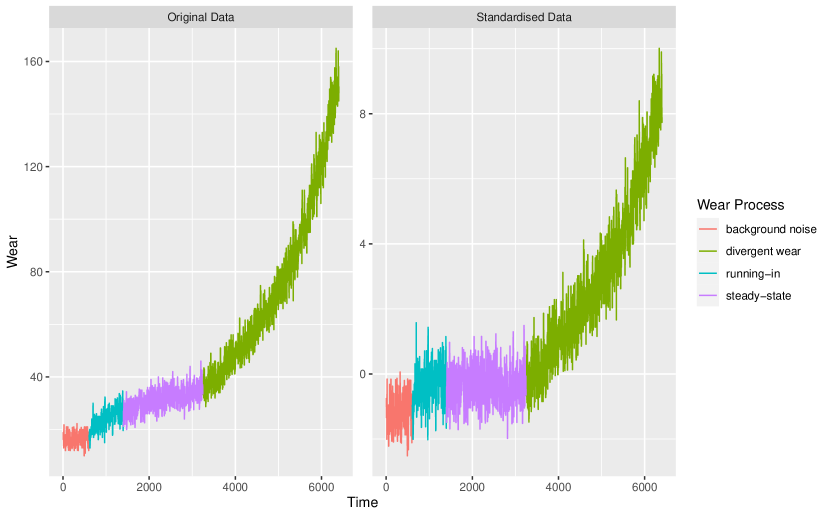
Figure 2: Heterogeneous time series data with regimes of different characteristic trends (left). See Section 3.1) for a detailed description about the tribological origin of the data. Also seen is a transformed version of the time series yielding a ’steady state’ in one of the regimes (right), as described in Section 3.2. Detecting change points into and out of stationarity will be seen to be simpler and adding to the power of the detection method.

The key idea of the proposed predict-and-compare framework is to apply a predictive model $\widehat{f}_{t}$ to input data from a time window $I_{t}$ of the immediate past, predicting a trend for future observations on a time window of the immediate future $J_{t}$. These predictions are then used to detect changepoints as significant deviations in the observed data from the predicted trend. This is illustrated in Figure 3, where the left part shows a case where a changepoint should be detected, and the right part illustrates a case without a change point. The process is described in detail as follows:

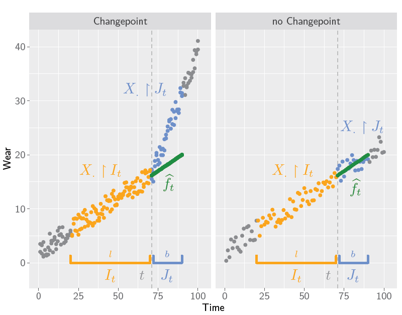
Figure 3: An illustration of P&C on data with a change point (left) and without a change point (right). The orange data points are used as input ($I_{t}$) for a predictive model $\widehat{f}_{t}$, whose predictions (green points) are then compared to the real data (blue points) on the prediction interval ($J_{t}$). The grey points are not used for the predictor $\widehat{f}_{t}$.

(1.) X and Y of the Predictive Model: Let $l$ and $b$ be the two positive integers which refer to the respective sizes of the input window $I_{t}:=\{t-l+1,\dots,t\}$, and prediction window $J_{t}:=\{t+1,\dots,t+b\}$, located around the discrete time value $t\geq l$. For a given sequence of real numbers $X\in\mathbb{R}^{\mathbb{N}}$ (the signal), the restrictions of this function on the positive integers to $I_{t}$ and $J_{t}$ will be denoted by $X\upharpoonright I_{t}$, and $X\upharpoonright J_{t}$, respectively. Two such vectors of size $l$, and $b$ are respective elements of the spaces of functions $\mathcal{X}:=\{X:I_{t}\to\mathbb{R}\}\cong\mathbb{R}^{l}$, and $\mathcal{Y}:=\{Y:J_{t}\to R\}\cong\mathbb{R}^{b}$.

(2.) Hopping Windows: We partition the positive integers greater than $l$ into disjoint intervals of width $b$, namely $\mathbb{N}=\uplus_{t\in T}J_{t}$ where $T=l+b\cdot\mathbb{N}$. We consider, for each $t\in T$, apart from $J_{t}$ the input window $I_{t}$ of width $l$. Moreover, for $J_{t}$ we consider an increasing sequence of growing sub-intervals $J_{t}^{j}=\{t+1,\dots,t+j\}$, of final maximal size $b$. The increasing times $s=t+j$ correspond to passing through the current moments in time within $J_{t}$.

(3.) Model training (fitting): We define a learning method $\mathcal{A}$ to be a map from a training data set $\mathcal{T}:=\{\langle X^{(i)},Y^{(i)}\rangle\}_{i=1}^{n}\subset\mathcal{X}\times\mathcal{Y}$ of size $n$ to a predictive model, i.e., a function $\widehat{f}_{t}:J_{t}\to\mathcal{Y}$ that allows to approximate $Y\in\mathcal{Y}$ with $\widehat{f}_{t}(X)$, also for new and previously unseen data points $X\in\mathcal{X}$. We perform the training of a learning method $\mathcal{A}$ once and use the training data set $\mathcal{T}$, where the vectors $X^{(i)}$ and $Y^{(i)}$ are taken from a different time series sample representative of the regular (change point free) part of $X$.

(4.) Predict and Compare: So, for the current time $s$, let the largest multiple of $b$ plus a single input window size $l$ smaller than $s$ be given by $t=l+b\cdot m$ for a suitable $m\in\mathbb{N}$. Then, the vector $X\in\mathcal{X}$ of values from the current input window is inserted into the predictive model $\widehat{f}_{t}:\mathcal{X}\to\mathcal{Y}$. The first $j$ values of the associated prediction $\widehat{f}_{t}(X)$ can then be compared to the first $j$ values of the vector of real observed data $Y$ on $J_{t}$. At each of these times $s=t+j$, a sequential test is run and either a detection is found, or the current time $s$ is incremented by one.

(5.) CUSUM in Compare step: The test we use in the Compare step is the CUSUM test (2). It acts as a map $C:\mathcal{Y}\times\mathcal{Y}\to\{\textrm{CP, No CP}\}$ to the possible outcomes of the test. In the following recursive expression, the CUSUM rule for upward changes is defined using the $\widehat{f}(j)$, the $j$-th element of the predicted time-series on $J_{t}$ as the target $\theta_{j}$:

$$S_{j}\;=\;\max(0,S_{j-1}+X_{j}-\widehat{f}_{t}(j)-k\,),$$ (4)

where, as in Step (2.), $t=\max\{r=b\cdot m+l\,|\,r\,<\,s\;,\;m\in\mathbb{N}\}$. In this way, CUSUM is ’assisted’ by the predictor $\widehat{f}_{t}$.

Remarks: In step (3.), we choose the training set and learning method according to the trends that we wish to consider as ’regular data’. It is the deviations of them that define a change point.

Q1 and Q2 are answered by these definitions: The trend is predicted by $\widehat{f}_{t}$ while the CP is detected by the help of the prediction-assisted CUSUM-rule.

In step (5.), we chose a specific test $C:\mathcal{Y}\times\mathcal{Y}\to\{\textrm{CP},\textrm{No CP}\}$ to decide about whether there are deviations between prediction $\widehat{f}_{t}$ and data $X\upharpoonright J_{t}$. The CUSUM test makes the whole detection method be online (see discussion, below - after the definition of the algorithm), and also because it provides a more exact location of the CP than the end of the prediction interval at the time of detection.

In addition to the classifier $C$, it is useful to consider a separate locator $L:\mathcal{Y}\times\mathcal{Y}\to J_{t}$ deciding about the time of occurrence of the CP. In the simplest case, it might coincide with the time of detection. In more sophisticated cases, the CP is placed somewhere in $J_{t}$. E.g., CUSUM uses the last time $s=t+j$ at which the indicator $S_{j}$ is zero bassevilleFAULTISOLATIONDIAGNOSIS2002 .

Definition 3: Predict and Compare Detector – A Predict-and-Compare detector (P&C) is a tuple $\langle\mathcal{A},\mathcal{T},l,b,C,L\rangle$ in which $\mathcal{A}:\mathcal{T}\to(\mathcal{X}\to\mathcal{Y}$) is a learning method defined on the training set $\mathcal{T}$ with values in the set of predictors mapping size-$l$ inputs from $\mathcal{X}$ to size-$b$ predictions in $\mathcal{Y}$, a classifier $C:\mathcal{Y}^{2}\to\{\textrm{CP},\textrm{No\,CP}\}$ deciding if a sub sample of $X$ of size $b$ is significantly deviating from a target sequence of the same size, and a locator $L:\mathcal{Y}^{2}\to J_{t}$ naming the estimated point in time of the CP.

Algorithm 1 P&C

1:procedure P&C($\mathcal{T},\mathcal{A},X,l,b,C,L$)

2:     $\widehat{f}_{t}=\mathcal{A}(\mathcal{T})$, the predictor

3:     for $t\in l+b\cdot\mathbb{N}$ do

4:         $I_{t}=\{t-l+1,\dots,t\}$, the current input window

5:         $J_{t}=\{t+1,\dots,t+b\}$, the current prediction window

6:         $\widehat{Y}=\widehat{f}_{t}(X\upharpoonright I_{t})$, the current prediction in $\mathcal{Y}$

7:         for $j\in\{1,\dots,b\}$ do

8:              $J_{t}^{j}=\{t+1,\dots,t+j\}$

9:              Let $\widehat{Y}\upharpoonright J_{t}^{j}$ be the vector of the first $j$ elements of $\widehat{Y}$.

10:              if $C(X\upharpoonright J_{t}^{j},\widehat{Y}\upharpoonright J_{t}^{j})==\textrm{No\,CP}$ then assume no CP in $J_{t}^{j}$

11:              else CP in $J_{t}^{j}$

12:                  Record $j$ as the point in time of the CP detection.

13:                  Record $c_{j}=L(X\upharpoonright J_{t}^{j},\widehat{Y}\upharpoonright J_{t}^{j})$, the CP location.

14:              end if

15:         end for

16:     end for

17:end procedure

Note that even though the algorithm is ’windowed’ into a discrete, non-overlapping, exhausting set of sub samples, it can still be used online because the comparison method $C(\cdot,\cdot)$ is online.

A true online detector can be applied at each accessible moment in time, i.e. for every moment at which the information belonging to the current time step becomes available. Sliding windows (such as in BFAST, cf. Section 2.2.3) or a cascade of fixed windows partitioning the time axis (as in our proposed detection algorithm) may be part of the approach without impairing the online property. While the current point in time makes the sliding window move continuously along, the cascading window approach let’s it wander through each consecutive interval, in which a parameter adaption is made. Nonetheless, the online property is completely retained, it is just a step-wise parameter-adjustment at the interfaces between two consecutive time windows.

Also, instead of changes in the location parameter, changes of the local dispersion of the signal can be controlled by CUSUM, e.g., by using the squared data $X_{t}^{2}$. There is classical work bissell2 on asymptotic optimality of such control chart problems from sequential modeling, and specific CUSUM rules for CPs in the variance of a signal variance . All of these can be realized as CP-types in the P&C framework by chosing the corresponding CUSUM test in the Compare step.

2.4 Analysis of artificial data

Before applying the P&C method to experimental data, we first use artificial data with different types of change points to allow for a broad orientation of what to expect. As described in Sect. 2.1, the process of physical wear in tribological systems undergoes several stages. As described in more detail in Sect. the condition of a journal bearing is monitored: Particles are coming loose of the pair of surfaces and initial abrasive wear due to physical contact in the run-in regime is followed by hydrodynamic effects including concatenation of the hydrodynamic contact-less lubrication. The transition into the divergent regime happens as particles amass and progressively damage the tribological pair given by bearing and shaft to the effect of there not being enough space for contact-less operation. The condition-monitoring involves counting radioactive decays proportional to the particles loosened by the wear process jech_radionuclide_2018 .

In order to get an idea of the power of P&C on such data, we generate time series samples with a simple model representing a change point from the run-in to the steady-state phase, as well as another change point from the steady-state to the divergent wear regime.

For the sake of simplicity and to just compare different forms of change points under different noise levels, we model the rate of wear, here, by

$$f(t)=a\cdot\lambda\cdot e^{-\lambda t}\;+\;c\;+\;d\cdot{\bf I}_{{}_{[t_{2},\infty)}}(t)\cdot\left(t-t_{2}\right),$$ (5)

where $\lambda,a,c,d\in{\bf R^{+}}$ AC1 . It is seen that after the decay of the exponential run-in process of amplitude $a$ to a (arbitrary, but fixed) fraction of one (at some time $t_{1}$) with rate $\lambda$ a phase of purely steady-state (’linear’) wear settles in and the rate progresses with constant magnitude $c$. The second change point occurs later (at $t_{2}$), when divergent (’quadratic’) cumulative wear establishes to be the dominant part.

To use the simplest renewal process with this time-dependent rate, we employ the time-dependent Poisson process Pstandard with intensity function which is given by $f(t)$ (usually called $\lambda(t)$, see Section 3.2) to simulate data shown in Figure 4. The lower part of this visualises the aggregation (by mean) of our two quality measures (Section 4.1) Fpc and ArlP for all data samples over different tuning parameter sets for Predict and Compare. A first impression shows that the data sample classes belonging to the three signal-to-noise ratios group into three clusters 1,2,3, in which group 1 has the lowest and group 3 the highest signal-to-noise ratio.

Overall the results from the aggregation of the two considered CPs (lower line of diagrams of Figure 4) show that the signal-to-noise ratio has a significant influence on the result regardless of the parameter settings for P&C: From the aggregated results, it can be observed that with increasing noise level

• for the divergent CP (into regime A) the Fpc is increasing, and the ArlP is first increasing and then decreasing, while

• for the CP from the run-in into the linear regime (into regime K) the Fpc is first decreasing and then increasing, while the ArlP is decreasing.
  

Observation (a) correlates with the intuitive notion that an increase in noise will increase the number of false positives. However, the time until detection being largest for the intermediate noise level is surprising. Similarly, observation (b) seems intuitively clear, as far as the final increase in Fpc goes. The decrease of Fpc and ArlP is unexpected.

This shows that a change in data may, on the one hand, reduce the power of the P&C detector, however may also improve the power of the trend predictor $\widehat{f}_{t}$, which leads to improvements both in terms of Fpc and ArlP. In Section 4.2, we investigate this systematically for a series of industrial data sets from tribological experiments.

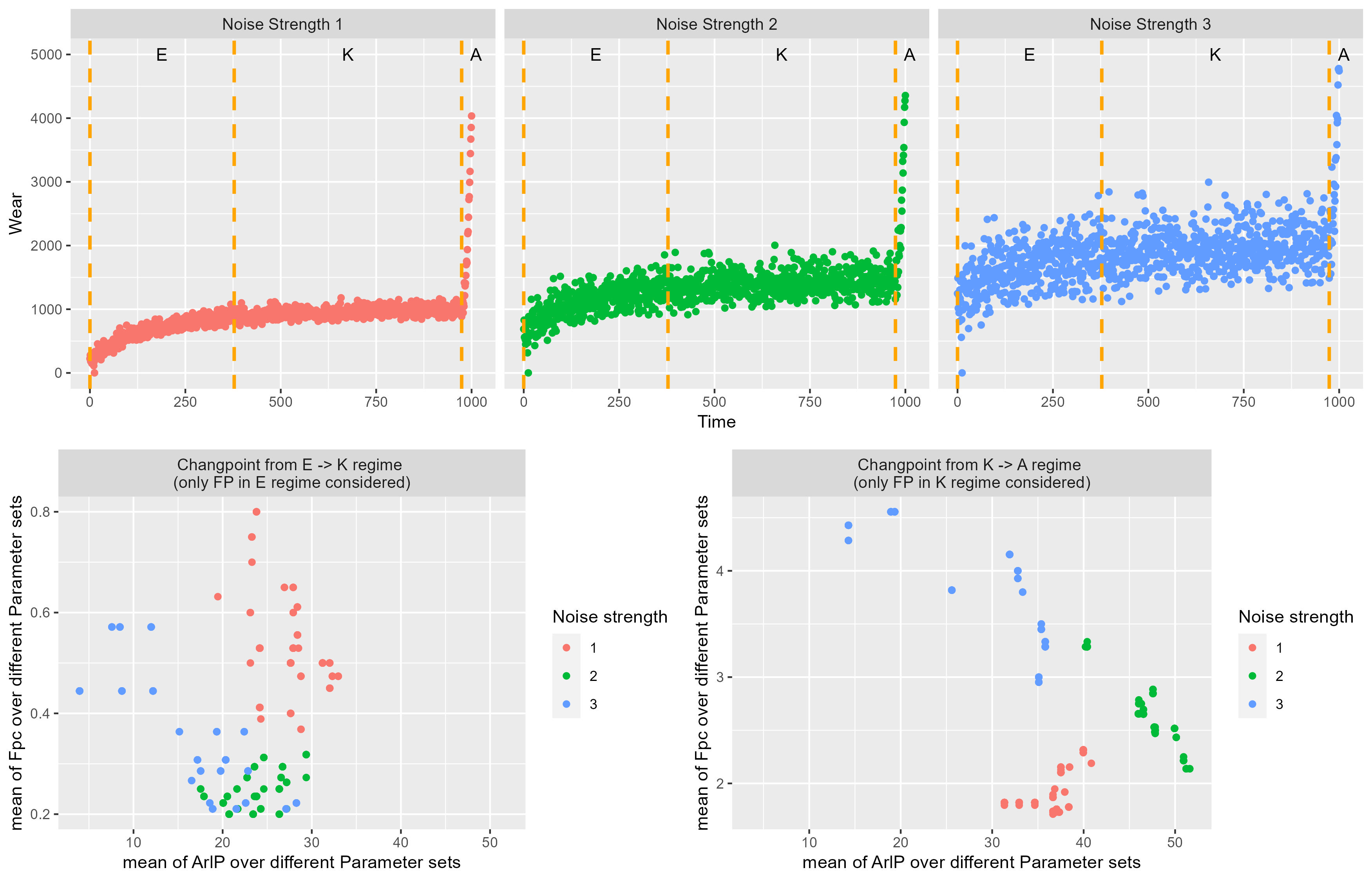
Figure 4: The top three plots show artificial data samples used to test the Predict and Compare method. The second and third vertical vertical dashed orange lines symbolize the CPs into regime K and regime A, respectively. Bottom: Plot shows the results of P&C with LSTM as the learning method applied to these two change points. The colours signify the respective strength of the signal-to-noise ratio from the diagrams, above. Each point represents the averaged results of P&C over different parameter sets for one data sample. The x-axis is the difference between the labelled and the found change point. False positive count (Fpc) is shown on the y-axis. Both averages are aggregated by using the mean.

2.5 Relation of P&C to other approaches

In this section, we compare the focus of the reference methods to P&C.

2.5.1 Classical CUSUM

The difference between classical CUSUM and Predict and Compare is that the target (or ’quality number’, pageContinuousInspectionSchemes1954a ) $\theta_{j}$ is replaced by the prediction $\widehat{t}_{t}(j)$. These predictions are subject to the result of the trained model $\widehat{f}_{t}$ and its input given by the data from the input window $I_{t}$. The predictions $\widehat{t}_{t}(j)$ are valid throughout a single prediction window $J_{t}$, and updated, as soon as the current time $j$ enters the next prediction window.

2.5.2 Break detection For Additive Season and Trend (BFAST)

In contrast to P&C, where the prediction $\widehat{t}_{t}(j)$ is compared to the real data points $J_{t}$ BFAST compares the parameters of the two models, using a ’Moving Sum’ (MOSUM)bfastMosum_zeileis_2005 . MOSUM is a statistical test designed to detect changes in model parameters. If MOSUM detects a parameter difference, the historic time period ($I_{t}$) is different from the monitored time period($J_{t}$) and a change point is detected. On the other hand, there is no change point if no difference is found as both periods are the same. Choosing the right size of the historic time period is vital for a successful comparison. BFAST offers an automated method to find a good value for $l$. Expert knowledge about the data can also be used to define $l$.

BFAST uses a historic and a monitoring time period similar to Predict and Compare. Therefore, it is interesting to compare those two methods.

2.5.3 Online Changpoint Detection (OCD)

The OCD aggregates a value gained from the data and compares it to a threshold to find change points, similar to P&C. For P&C, this value is the sum of differences between the real data point and a predicted data point, which, if it crosses a threshold, indicates a change point. OCD calculates the diagonal statistic and off-diagonal statistic for the threshold comparison.

2.5.4 Bayesian CPD

The Bayesian approach to online change point detection taken in AdamsMacKay potentially using more than one latent state employs updating the posterior distribution of the run-length $r_{t}$ during every time step using the hazard function $H(t)$. If the Hazard function is constant, the run-length distribution becomes geometric and independent of the observed data (see diego_2020 , Sect. 2.2). Similarly, if $H(t)$ is bounded from below by a positive constant $c$, then the distribution of the residual time $l_{t}$ before a CP occurs is also of the form $c(1-c)^{l_{t}}$. This situation is given, if the data before the occurring CP is stationary. This occurs in our use case after the standardization transformation has been applied (see Fig. 7, the stretches before the green (divergent) regime).

Bayesian methods such as that of Adams and MacKay are fully online, helping the time until detection become small. Very small Hazard rates, on the other hand, become hard to determine precisely. Experimental situations in which such very low rates of occurring CPs enter as parameters into the modeling with the hazard function are therefore more difficult to estimate exactly.

3 Experiment

3.1 Data for Experiments

For the evaluation of the CPD methods/strategies, data sets of real experiments have been deployed within this paper. Within these experiments, the performance of machine parts is examined through a bench test. The wear of the specific and critical machine part is continuously monitored via an in-situ technique based on radioactive isotopes jech_radionuclide_2018 .

For this wear measurement, the critical machine part is labelled with radioactive isotopes via thin layer activation brisset_radiotracer_2020 . Due to the frictional contact wear particles are generated, which are transported by the lubricant circuit to a gamma ray detector. Through the measurement of the activity of the wear particles in the lubricant and the combination with the knowledge about the isotope depth distribution in the labelled machine part, the amount of wear can be calculated.

There is a shift of time, when a wear particle is generated until it reaches the detector and is detected. This time shift is in the range of a few minutes and consequently much faster than changes in the wear behaviour. Nevertheless, this time shift must be considered for comparison of different measurement methods (e.g., a rise of temperature) for in-time recognition of change points in machine performance.

The applicability of AI methods for CPD is dependent on the data provided by the measurement and thus the specific characteristics of the measurement method must be considered. For the applied continuously monitoring wear measurement the statistics of radioactive decays must be regarded as part of the signal scattering/noise. Furthermore, wear particles are sometimes not distributed homogeneously in the whole lubricant circuit and so fluctuations of wear particle concentration may occur in the detector volume, which is a certain fraction of the whole circuit. These effects will be considered by specific standardization of the Poisson process (see therefore Section 3.2).

The fast detection of the change points– for example when divergent wear starts – is crucial for wear testing but also for maintenance of machine parts in the production process. If the divergent wear change point can be detected timely and with high accuracy, the origin and cause of the wear can be investigated (especially interesting when testing prototype parts) and expansion of the damage can be limited in the production processes. In this sense, timely is referred to as being faster than the occurrence of the final damage but also being faster than other detection methods which are currently used. High accuracy is referred to issuing a warning (signal) when divergent wear occurs. Divergent wear should not be overlooked by the CPD, but warnings without actual cause should also be avoided.

In total, 4 different wear phases can appear in the 5 uni-variate time series datasets used in this paper (Figure 5). One phase is called experiment paused, which refers to times when no new particle from the experiment reaches the detector. At the beginning of each dataset represents the stationary background noise detected by the detector. Another phase is the non-stationary running-in or run-in wear phase, where the increase in the wear volume starts high and reduces over time. This behavior is only visible in dataset 1 and 3. In the other three datasets, this is hidden by the noise. In the constant or steady-state wear phase, the increase is linear. In the fourth phase, the divergent wear, the wear volume increase is more than linear. The transition between two of the four phases is a change point.

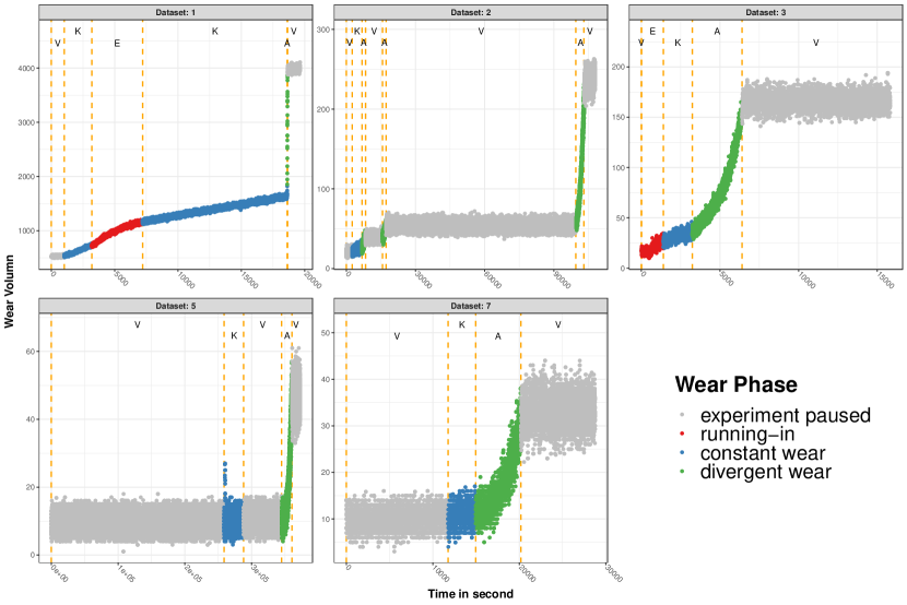
Figure 5: The five different data sets with divergent wear used for evaluating the different change point methods.

3.2 A standardizing transformation

P&C is evaluated with tribological data (Figure 5), which due to the nature of the tribological experiments (see Section 3.1), are noisy. To increase the detectability of the wear phase changes in the noisy data, a transformation is applied. For this transformation, we look at the cumulative sum of a noisy, and itself increasing function $f(t),t\in{\bf R}_{+}$ (representing the rate of wear over time $t$) with the independent but increasing in its standard deviation noise $W_{t}$. This leads us to a model for the wear per unit time $X_{t}$:

$$X_{t}\;\;\;=\;\;\;f(t)\;\;+\;\;W_{t}\;\;+\;\;I_{t}.$$ (6)

$W_{t}$ and $I_{t}$, and so also $X_{t}$ are $t$-indexed random processes (i.e. for each $t\geq 0$ they are functions on a suitable probability space), and $f:[0,\infty)\to[0,\infty)$ is ’deterministic’. The function $t\mapsto I_{t}$ is either zero, or, represents a non-vanishing anomaly describing the structural change following the change point.

We assume that within the regime of steady-state wear, there is arithmetic growth of the wear rate, namely $f(t)=b\cdot t^{\nu}$, where $b,\nu>0$. Given any estimator of $b$ and $\nu$ trained on data $\mathcal{T}:=\{X_{i}\}_{i}^{n}$ called $\widehat{b}$ and $\widehat{\nu}$, respectively:

1:procedure Standardization($X_{t}\mathchar 24635\relax\;\,\mathcal{T},t_{0},t$)

2:     Determine $\widehat{\nu}$ using $\mathcal{T}$.

3:     Determine $\widehat{b}$ using $\mathcal{T}$.

4:     Define $\widehat{\lambda}(t):=\widehat{b}\cdot t^{\widehat{\nu}}$

5:     Define $\widehat{Z}(t):=\frac{X_{t}\;\;-\;\;\widehat{\lambda}(t)}{\sqrt{\widehat{\lambda}(t)}}$

6:     return $\widehat{Z}(t)$

7:end procedure

The formula for $\widehat{Z}(t)$ is chosen with the idea that they are realisations of an inhomogeneous Poisson Process with an intensity function $\lambda(t)$, which represents the local mean and variance. Therefore, the standard deviation estimate results from the square-root of $\widehat{\lambda}$ in the standardization.

Now, estimating $b$ and $\nu$ follows the following argument (which we used in the calculation for the experiment in Section 4.2): Assume that there is an estimator $\widehat{\Lambda}$ of $\int_{t_{0}}^{t}\lambda(s)ds$. Then, it is clear that if $t$ becomes large, under our assumption about $f(t)$, (6), and the fact that because of ${\bf E}[W_{t}]=0$, we have $f(t)=d/dt{\bf E}[\int_{t_{0}}^{t}X_{s}ds]=\lambda(t)$, $\frac{\log\Lambda(t_{0},t)}{\log t}\to\nu+1.$ Therefore, we choose as the estimation procedure

1:procedure Estimate-Trend-Parameters($\mathcal{T},t_{0},t$)

2:     Compute $\widehat{\Lambda}(t_{0},t):=\sum\limits_{j=t_{0}+1}^{t}X_{j}$ with the data in $\mathcal{T}$.

3:     $\widehat{\nu}_{t}:=\frac{ln(\widehat{\Lambda}(t_{0},t))}{ln(t)}\;-\;1$

4:     $U_{t}:=t^{\widehat{\nu}}$

5:     Call $\widehat{b}$ the estimated coefficient $b$ of the linear regression model

$$X_{t}=b\cdot U_{t}+\varepsilon_{t}.$$

and use the data in $\mathcal{T}$ for fitting this model.

6:     return $\langle\widehat{\nu},\widehat{b}\rangle$

7:end procedure

The standardization also works online in the sense that up to every current point in time $t$, the available data $\{X_{s}\}_{s\in[t_{0},t]}$ is input to Estimate-Trend-Parameters($\cdot,t_{0},t$). Figure 6 shows the effect of this transformation on the run-in, the intermediate steady-state wear, and terminating divergent wear regime. As in the intermediate regime, there is a constant arithmetic form of growth of the underlying trend function $f(t)$, the standardized data is (close to) a stationary signal, most of that regime. It is seen that there is a run-in phase in the beginning of the intermediate phase before stationarity ’kicks in’. Then, however, it is seen that the growing dispersion of the original data is transformed into a sequence with locally constant standard deviation. In spite of this standardization of the steady state regime, the change point into the divergent regime in the end is still clearly marked by a visible change point.

The key feature of the standardization may be considered to be line 3 of the Estimate-Trend-Parameters procedure. Here, the estimator $\widehat{\nu}_{t}$ is chosen for functions of arithmetic growth, i.e., of the type shown in line 4 of the Standardization procedure. This is the type of growth rate expected from the steady state regime in the original (non-standardized) data set.

A characteristic shape of the transformed sequence is visible in the first and third of the five used data sets shown in Figure 5 and Figure 7. The data of the red run-in phase is transformed from an increasing shape into a curved non-monotonic shape, which is followed by the eventually stationary stretch of the steady state regime. The green stretches represent the divergent wear behavior which is also in standardized form clearly distinguishable from the steady-state wear regime, before.

We conclude that the standardization yields a transformation into the eventually stationary form for the steady state regime, while the change points into and out of this interval are still clearly detectable by the change point detector. This will become more clear in the discussion of the results (see Section 4.4): Our detector defined by P&C sees the run-in to steady state change point clearer than the reference methods. At the same time, the strong change point at the beginning of the divergent wear regime typically (among the five different experimental wear data sets considered) remains most clearly detectable, even though the standardized data is used.

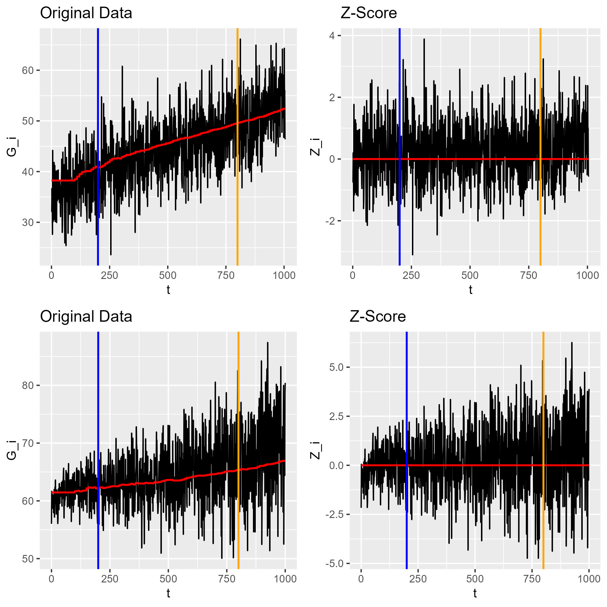
Figure 6: Examples of the standardization (right) of typical wear curves (left) under strong noise with run-in, steady-state-, and divergent wear. Both simulations in the left column show simulated inhomogeneous Poisson Processes (red line being the intensity function). The standard deviation increases proportional to the square-root of time. The simulation in the upper row has the starting point moved to negative values, which is why the increase is not as clearly visible as for the simulation in the lower line. However, it is typical for the real experimental data, and so the effect of the standardization is demonstrated, here.

Figure 7: The same 5 data-sets as in Figure 5 standardized with our standardization method Section 3.2. It is visible, that the regimes of linear increase of wear yield a stationary z-score, after some ’run-in’ period. Note that the standardization is calculated at every instant in time only with values available up to that instant, as is required by a full online detector.

3.3 Comparative Experiments

All experiments were conducted with R. One experiment can be defined as using a method with a certain parameter set on one dataset. The change points found by an experiment were saved and later used to define the effectiveness of each method by calculating two criteria, see Section 4.

Five different tribological datasets (Figure 5) are used to evaluate and compare the change points methods. All these datasets include a divergent wear part. As part of the preprocessing, these datasets are standardised using the method described in Section 3.2 (datasets after the standardisation Figure 7). The methods used in this part of the paper are BFAST, Bayesian, CUSUM, ARIMA used with CUSUM and LSTM used with CUSUM. Additionally, a simple ’baseline’ is created by sampling random points from the datasets and treating them as change points. Recognizing the inherent independence and uniformity of the sampling procedure, it is apparent that conditioning the sampling based on a predetermined quantity of false positive finds can be effectively realized by terminating the sample collection process upon reaching the desired number of false positives. We choose the number of false positive finds to be either 0 or 10 or the average maximal number of false positives found by other methods for one dataset. These three cases are reasonable because 0 false positives are the desired outcome for our use case. 10 is the maximum allowed number of false positives due to the use case. The last is interesting for observations based on the other quality measurement used to compare all methods (see Section 4.1). To avoid the strong influence of an outlier that could happen by executing the sampling process only once per data set and number of false positives, each process is repeated 100 times. The resulting quality measurements are then averaged before being used for comparison. This baseline can be seen as a simple method to show that a more complex method is necessary for this problem.

For the first four methods and the baseline, no further preprocessing steps needed to be done before the experiment could be run.

More steps needed to be taken before the experiment for the ML-assisted predict and compare method. As the ML method, LSTM is used. This LSTM needs to be trained before it can be used for prediction (details in Section 3.3.6).

For each method multiple experiments were run with different parameter sets. How we defined the ranges of the parameter is explained in Section 3.4. The packages and parameters used in the experiments are described in the following subsections.

3.3.1 BFAST

For the implementation of the BFAST method the eponymous package BFAST verbesselt_near_2012 was utilised. This package implements different functions. The bfastmonitor function is the implementation of the online version of BFAST decribed in verbesselt_near_2012 .

For the following parameters $minHist$, $histFact$, $h$ and $level$ different values were tested in the experiments. The first two parameters define the length of the stable histroy accessable to bfastmonitor. These parameter effect $history$ parameter of the bfastmonitor, which indicates the start of the stable history period in the data available to the BFAST online function. $histFact$ defines a percent value of the available history that is stable and $minHist$ ensures that there is at least a certain amount of history available to the function. The maximum amount of history was also limited but never changed during the experiments.

$h$ specifies the bandwidth of the mosum process. The range of $h$ is between 0 and 1 as the bandwidth should be defined relatively to the data available. $level$ sets the probability of that a type 1 error occurs. $level$ and $h$ are parameters used by bfastmonitor.

3.3.2 Bayesian

The experiments on the Bayesian online method where conducted with the online CPD method found in the ocp AdamsMacKay package. During the experiments the threshold parameter called $cpthreshold$ was varied. This parameter defines the height of the run length probability which if exceeded leads to a change point being detected.

3.3.3 OCD

For OCD, an implementation in an R Package of the same name exists. There the sensitivity of the detector is regulated by two thresholds diag and offDiag, one for the diagonal statistic and one for the off-diagonal statistic calculated by OCD, respectively. For the change point detection, the $getData$ function is used. This function calculates the statistics and checks if the results are above (change point found) or below the chosen threshold. The package further provides a method to estimate the parameters necessary for the calculations. This is done at the beginning and after each found change point.

3.3.4 CUSUM

For our experiments with the CUSUM change point detection method the CUSUM function from the qcc package qcc_2004 was used. For this change point detection method only one parameter was tested with different values, the $decision.interval$ ($desInt$). This parameter is the same as the $\lambda$ parameter named in Section 2.2.2, the qcc package just uses a different name. The $decision.interval$ controls the sensitivity of CUSUM. A high value for the decision.interval leads to few change points detected and a low value to many detected change points.

3.3.5 ARIMA CUSUM

Here CUSUM from qcc was also used. For the ARIMA part the implementation from the forecast forecast_2008 ; forecast_2022 package was used. The function used is called auto.arima, this method decided automatically the order of the ARIMA model that fits the data provided best. As we work with heterogeneous data, where in different experiment stages different wear behavior can be observed, it was decided to let the auto.arima function fit the right model for the data. This fit is only performed at the beginning and after each detected change point as at those points we need to fit the model to a new behavior. Furthermore, fitting the ARIMA model only at those points leads to faster results. The ARIMA part adds no parameters that need to be considered during the experiments, therefore only the $decision.interval$ ($desInt$) value is varied during the experiments.

3.3.6 LSTM CUSUM

The qcc implementation of the CUSUM method was used once more. The implementation of the LSTM part was done by utilising the well-known Keras kerasR_2017 package for R. LSTM_model_fit, predict and modelFit are only some of the functions used for the implementation. Additionally to the $decision.interval$ ($desInt$) there are two more parameters that need to be considered during the experiment. The length of the input window (number of input neurons for the LSTM)($nh$) and the size of the future window (number of output neurons for the LSTM)($nz$).

Differently to all the other methods mentioned above, the LSTM needed to be trained before it can be used successfully for a prediction and in an experiment. Therefore, it was necessary to prepare training data from tribological experiments without divergent wear. This choice also helps to prevent overfitting, as the data sets used for training are different from those in the experiments. Due to the missing divergent wear part, these data sets are not used to evaluate the change point detection methods. The LSTMs were trained with the z score standardized training data sets. The best number of epochs and the batch size were determined by comparing the results of the prediction accuracy for a training and validation data set. The predictive power of the LSTM hasn’t been optimized over the number of training samples. However, the size was chosen large enough (500), so as to recognize the typical trend patterns before the specific CPs (run-in behavior, linear increase of steady-state regime). The trained LSTMs were then used together with CUSUM in the experiments to detect change points in the tribological data with divergent wear (Table 3), and constant wear after the run-in (Table 6).

3.4 Parameter selection for Experiment

For the experiments, different ranges of parameters for each method were used. For all the parameter ranges, the same criteria apply. Inside the chosen range, all settings have to find at least one change point for at least one dataset and less than 1000 change points for at least one data set. To find those borders we tested the different method with extreme values in the parameters. After defining the borders, step sizes for each range were defined. Every step corresponds with a parameter value which was tested. For those method with multiple parameter (BFAST and LSTM CUSUM) the experiment was conducted for each parameter value combination.

Furthermore, some of these parameters (nh, nz and minHist) are responsible for the amount of data the method has access to. For these parameters, another criteria for the boundary was considered. Due to the nature of the data, the first 600 data points don’t have any change points. Therefore, they can be used safely as historical data without the risk of overlooking a change point.

4 Results and Comparison

4.1 Quality measures

This chapter shows the results of the experiments described in Section 3. We first note that typically the type I error measure is $\textrm{ARL}_{0}$, the average run length between two false positive detections (average run length in control). The type II error is usually measure by the average time between actual occurrence and detection of a change point (average run length out of control, denoted by $\textrm{ARL}_{\Delta}$, hinkley70 ). Note that for unlabeled data, the estimator of this measure is usually defined by the time between the estimated occurrence of the change point and its detection time, which entails another source of uncertainty versus our case of known ground truth change point positions in time).

Instead of using $\textrm{ARL}_{0}$, we use the number of false positive events (detections which do not correspond to real change points (labelled by experts according to the definition given in Section 3.1)) before the occurrence of a specific change point, which will be called Fpc. This choice arises from the notable variations in observation counts across our datasets (see table 1), rendering the actual count of false positives a more sensible gauge of quality than an associated probability-expressing ratio.

Table 1: This shows an overview of the length of the different wear phases in each dataset and the total length of each dataset. It can be seen that the length of the phases vary significantly between the different datasets.

dataset	running-in wear	constant wear	divergent wear	experiment paused	all Datapoints
1	4005	13596	25	2010	19636
2	0	4239	6605	96871	107715
3	802	1842	3158	10019	15821
5	0	29237	15515	327592	372344
7	0	3191	5233	20351	28775

For the type II error, we employ an estimator based on $\textrm{ARL}_{\Delta}$. To increase the comparability between the different datasets, the number of discrete time steps between the label and the detection is transformed into a percentage value. The basic value for the calculation is the number of data points of the wear phase, which begins with the labelled change point corresponding to the found change point. Figure 8 shows the result of a change point detection method applied to dataset number 3. To calculate the ArlP of the found change point between the constant and the divergent wear phase (found CP K$-$>A) for this example. One needs the position of the change point (3476) and the length of the divergent wear phase (3158), which is defined by two labelled change points, one between the constant and the divergent wear phase (labelled CP K$-$>A) and one between the divergent wear and a pause in the experiment (labelled CP A$-$>V). Therefore the ArlP is 7.32. The Fpc for this change point is two because the two additional false positive detections after the detected change point are not counted due to the online setting of the scenario in which the experiment is stopped in case of the detection of this change point, and therefore, those change point would not be detected.

The following applies to all discussed results. The ArlP and Fpc were only calculated for the results of runs that found at least the change in the divergent wear.

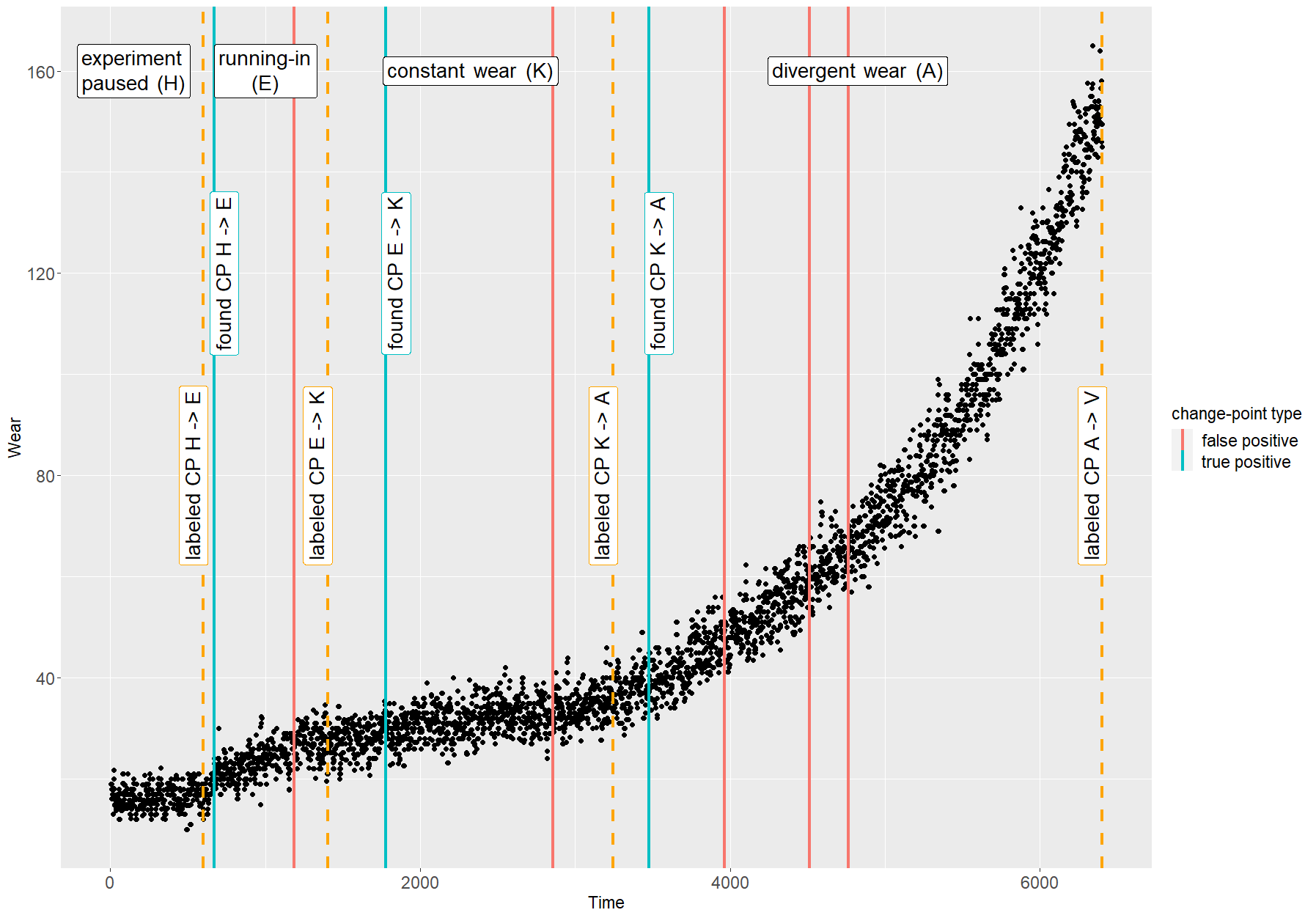
Figure 8: The multiple vertical lines indicate either change points labelled by experts (orange), true positive (blue) or false positive (red) detections, in dataset number 3.

4.2 Results

Table 2 gives an overview in which each method is independently summarized in terms of its best and worst result. A first look at these values shows for the false positives that

• for at least one parameter set, ARIMA CUSUM, CUSUM, LSTM CUSUM and OCD produced very few or non false-positives;

• looking at the worst-case scenarios regarding the Fp criteria, ARIMA CUSUM is still the method with the least amount of false positives;

• another interesting observation is that all method have their highest Fpc for the $5^{t}h$ dataset.

In terms of the ArlP,

• OCD is the fastest method to detect change points, closely followed by BFAST, LSTM CUSUM, CUSUM and Bayesian.

• The Predict and Compare methods (ARIMA CUSUM and LSTM CUSUM) are the fastest result in the case of data set 3, while the other methods all have the fastest results at data set 7 (except for OCD for which data set 5 delivers the fastest result).

Looking at the minimal and maximal values of the criteria separately gives an understanding of the boundaries of the method’s performance. The separate consideration of the criteria means that the lowest value of one criterion does not automatically correspond with the lowest criteria of the other criteria. To find the best-performing method, it is important to find the run with the best combination of Fpc and ArlP. The best combination of these two metrics depends on the specific scenario in which the change point detection is being used. In some scenarios, a low Fpc is more important than a low ArlP. In others, the fast detection of change points is so important that a higher Fpc is acceptable. In the scenario, we look at in this paper, a low number of false positives is important (up to 10 is acceptable), even if it might lead to a longer detection time.

Table 2: This table shows the minimal and maximal value of the false-positive count (Fpc) and the average run length percent (ArlP) per method and dataset.

Method	Dataset	min Fp	max Fp	min ArlP	max ArlP
	1	0	20	30.50	82.45
	2	0	17	18.76	70.75
	3	0	10	1.11	63.18
	5	0	375	14.70	78.02
ARIMA CUSUM	7	0	17	21.48	88.80
	1	0	169	44.5	48.4
	2	0	37	9.12	46.9
	3	0	124	3.16	49.9
	5	0	2136	0.71	25.1
Baseline	7	0	152	3.68	42.6
	1
	2	218	1091	1.95	7.66
	3	102	255	3.99	10.10
	5	581	2135	0.10	0.10
Bayesian	7	81	338	0.06	0.63
	1	0	118	2.52	98.44
	2	5	265	0.72	64.17
	3	0	18	0.16	80.66
	5	39	2282	0.01	55.68
BFAST	7	15	97	0.00	75.33
	1	2	1044	2.52	70.46
	2	0	884	0.72	38.97
	3	0	185	0.06	21.38
	5	0	8101	0.13	77.65
CUSUM	7	0	830	0.00	78.50
	1	4	236	2.52	78.46
	2	0	619	0.41	92.82
	3	0	123	0.19	92.03
	5	0	1235	1.94	77.48
LSTM CUSUM	7	0	151	0.61	91.63
	1	0	158	0.06	90.4
	2	0	79	0.02	95.2
	3	0	29	0.10	97.1
	5	0	3379	0.01	94.8
OCD	7	0	145	0.44	79.6

Table 3 shows the best runs per dataset and method where the Fpc was lesser than or equal to 10. In case more than one candidate per data set and method was found, the following rule was applied: Smallest Fpc and then smallest ArlP. ((Table 3) show the result for the opposite rule). The result shows that

• for datasets 2, 3, 5 and 7 the LSTM CUSUM is the best performing one;

• for dataset 1, BFAST is the best performing one;

• ARIMA CUSUM, CUSUM,OCD and LSTM CUSUM have at least one parameter setting that works well for each dataset.

The difference between dataset 1 and the other datasets lies in the very short divergent wear phase (25 data points) compared to the others.

Table 3: This Table shows the best result per dataset and method under the condition that 10 false-positives were found at max. Change point considered here (only): Divergent Wear.

Method	Dataset	Fpc	ArlP	Parameter
BFAST	1	0	14.51	minHist: 175, histFact: 0.30, h: 0.50, level: 0.001
ARIMA CUSUM		0	38.49	desInt: 100
OCD		0	42.5	diag: 210001, offDiag: 4100001
CUSUM		2	26.50	desInt: 400
LSTM CUSUM		4	78.46	desInt: 400, nh: 100, nz: 20
LSTM CUSUM		0	1.94	desInt: 300, nh: 500, nz: 100
CUSUM		0	4.72	desInt: 400
ARIMA CUSUM		0	18.69	desInt: 350
OCD		0	36.1	diag: 4201, offDiag: 156001
Baseline		0	52.0
BFAST	2	5	64.04	minHist: 175, histFact: 0.25, h: 0.50, level: 0.005
LSTM CUSUM	3	0	0.22	desInt: 120, nh: 600, nz: 50
OCD		0	1.71	diag: 101, offDiag: 501
CUSUM		0	5.29	desInt: 130
ARIMA CUSUM		0	22.99	desInt: 200
Baseline		0.1	43.4
BFAST		0	80.66	minHist: 50, histFact: 0.25, h: 0.50, level: 0.002
LSTM CUSUM		0	48.39	desInt: 125, nh: 600, nz: 40
Baseline		2.35	50.0
ARIMA CUSUM		0	51.78	desInt: 450
OCD		0	53.1	diag: 210001, offDiag: 4100001
CUSUM	5	0	77.65	desInt: 300
LSTM CUSUM	7	0	14.56	desInt: 140, nh: 600, nz: 200
OCD		0	15.3	diag: 4201, offDiag: 6001
ARIMA CUSUM		0	36.54	desInt: 325
CUSUM		0	37.07	desInt: 150
Baseline		1.11	43.9

The next question is to find the one parameter set that works best for all data sets combined. According to Table 4, in this sense

• ARIMA CUSUM has the best overall performance;

• the best overall result for LSTM CUSUM has a larger Fpc than $50$.

The Fpc and ArlP values for each parameter set and method were summarised to generate this table. Therefore, The threshold of 50 comes from the Fpc threshold (10) initially being multiplied by the number of data sets (5). However, in order to also include a LSTM CUSUM result, the threshold used in Table 4 was shifted further up to 150.

Table 4: Results grouped by parameter set over all datasets. With 150 false positives found at max, at least the divergent-wear change was found.

Method	$\Sigma$ Fpc	sd Fpc	$\Sigma$ ArlP	Sd ArlP	Parameter
ARIMA CUSUM	1	0.45	252.94	17.98	desInt: 725
ARIMA CUSUM	1	0.45	287.47	20.99	desInt: 700
ARIMA CUSUM	2	0.89	265.22	16.73	desInt: 650
ARIMA CUSUM	2	0.89	269.23	17.38	desInt: 675
ARIMA CUSUM	4	1.10	187.53	17.09	desInt: 575
ARIMA CUSUM	4	1.10	187.57	17.09	desInt: 600
ARIMA CUSUM	4	1.10	225.57	15.40	desInt: 625
CUSUM	4	1.79	237.08	28.96	desInt: 300
ARIMA CUSUM	7	1.14	218.48	13.64	desInt: 525
ARIMA CUSUM	7	1.14	218.48	13.64	desInt: 550
CUSUM	8	2.61	179.75	27.35	desInt: 200
ARIMA CUSUM	8	1.52	225.56	19.27	desInt: 500
CUSUM	10	2.92	142.47	18.94	desInt: 180
CUSUM	16	3.56	93.56	13.34	desInt: 160
CUSUM	29	7.50	91.55	13.18	desInt: 140
Baseline	29.3	4.99	235	18.6
CUSUM	62	18.46	70.65	12.92	desInt: 120
LSTM CUSUM	143	34.52	146.26	23.08	desInt: 120, nh: 400, nz: 50

Table 5: Results grouped by parameter set over the datasets 3,5 and 7 with 30 false positives found at max. Change Point: Divergent-wear.

Method	$\Sigma$ Fpc	sd Fpc	$\Sigma$ ArlP	Sd ArlP	Parameter
CUSUM	0	0.00	175.60	33.85	desInt: 300
ARIMA CUSUM	1	0.58	118.17	11.22	desInt: 725
ARIMA CUSUM	1	0.58	156.82	27.42	desInt: 700
CUSUM	2	1.15	99.09	24.27	desInt: 180
CUSUM	2	1.15	135.29	33.51	desInt: 200
ARIMA CUSUM	2	1.15	142.71	21.13	desInt: 650
ARIMA CUSUM	2	1.15	142.73	21.13	desInt: 675
Baseline	3.57	1.13	137	3.69
ARIMA CUSUM	4	1.15	109.08	13.00	desInt: 625
ARIMA CUSUM	4	1.15	110.11	13.82	desInt: 575
ARIMA CUSUM	4	1.15	110.14	13.82	desInt: 600
ARIMA CUSUM	6	1.00	110.14	13.76	desInt: 525
ARIMA CUSUM	6	1.00	110.14	13.76	desInt: 550
CUSUM	7	4.04	55.17	16.73	desInt: 160
ARIMA CUSUM	7	1.53	104.32	15.46	desInt: 500
LSTM CUSUM	11	4.04	133.92	12.58	desInt: 120, nh: 400, nz: 50
LSTM CUSUM	15	5.00	80.73	22.79	desInt: 125, nh: 500, nz: 50
Baseline	17.8	4.74	102	6.10
CUSUM	19	10.12	53.77	16.64	desInt: 140
LSTM CUSUM	19	7.09	80.73	22.79	desInt: 120, nh: 500, nz: 50
LSTM CUSUM	24	8.00	150.74	27.23	desInt: 100, nh: 500, nz: 40
LSTM CUSUM	25	10.41	86.45	21.54	desInt: 110, nh: 400, nz: 50
OCD	26	15.01	88.54	18.11	diag: 4201, offDiag: 100000000
OCD	29	8.50	136.87	29.75	diag: 1201, offDiag: 100000000

By restricting our observations to data sets 3, 5, and 7 we obtain the results of Table 5 in which correspondingly an Fpc of at most 30 was allowed. We observe that

• there are more results (due to fewer Fpc exceeding the threshold of 30);

• CUSUM wins, but ARIMA CUSUM is comparable in its performance.

• LSTM CUSUM is included within the cases with Fpc counts less than 30.

This allows recognizing data sets 3, 5, and 7 similar in the sense of methods with single parameters sets being universally applicable on them.

Finally, we observe for the change point into the steady-state wear regime (instead of the divergent wear regime) we see from Table 6 that

• the Predict and Compare Methods are the most successful on data sets 1 and 5;

• ARIMA CUSUM always appears in the cases with a Fpc of less than 10.

The fact that in this table (Table 6) some methods don’t appear in the lost of specific data sets is related to the fact that the change point into the steady-state wear regime does not occur for some parameter sets from Table 3.

Table 6: This Table shows the best result per dataset and method under the condition that 10 false-positives where found at max. Change point considered here (only): Constant Wear.

Method	Dataset	Fpc	ArlP	Parameter
ARIMA CUSUM		0	3.61	desInt: 75
OCD		0	20.0	diag: 4201, offDiag: 156001
Baseline		0.17	42.7
BFAST		1	0.40	minHist: 175, histFact: 0.30, h: 0.50, level: 0.002
CUSUM		1	14.14	desInt: 300
LSTM CUSUM		7	67.40	desInt: 300, nh: 50, nz: 100
Baysian	1	9	3.74
OCD		0	8.87	diag: 501, offDiag: 501
CUSUM		0	9.55	desInt: 110
ARIMA CUSUM		0	18.45	desInt: 125
Baseline		0.1	50.2
BFAST	2	3	0.19	minHist: 200, histFact: 0.30, h: 0.50, level: 0.005
OCD		0	0.69	diag: 1201, offDiag: 4201
ARIMA CUSUM		0	20.77	desInt: 325
Baseline		0.03	47.4
BFAST		2	2.05	minHist: 225, histFact: 0.30, h: 0.50, level: 0.001
CUSUM		3	37.27	desInt: 80
LSTM CUSUM	3	6	13.50	desInt: 100, nh: 200, nz: 50
LSTM CUSUM		0	3.23	desInt: 110, nh: 500, nz: 40
CUSUM		0	5.58	desInt: 300
Baseline		2.26	42.4
ARIMA CUSUM	5	4	94.04	desInt: 150
OCD		0	62.5	diag: 4201, offDiag: 4201
ARIMA CUSUM		0	71.64	desInt: 250
CUSUM		0	74.65	desInt: 150
Baseline		1.03	56.1
BFAST		2	67.97	minHist: 200, histFact: 0.25, h: 0.50, level: 0.001
LSTM CUSUM	7	2	88.97	desInt: 175, nh: 200, nz: 100

4.3 Discussion

We first note that P&C  as a fully online working algorithm, it can -in principle- handle data needing large prediction windows (cf. large $\varepsilon$-values in the $\varepsilon$-realtime algorithms in amin_2017 ) such as those with gradual changes (slow onsets of trend-changes) well, in the sense that the time until detection (and therefore, on average, the Arl) even for CPs occurring at the beginning of these windows can be small and not on the order of magnitude of the prediction window size. Furthermore, since hopping windows are used (not sliding), the multiple testing problem of sliding windows with non-empty intersection is avoided and taken care of in the sense of the sequential CUSUM test. In this sense, there are no problems of ambiguous results of different CP-results of overlapping sliding windows.

Therefore, we arrive at noting that with the right tuning, Predict and Compare works well for change points with gradually developing onsets of the anomalies (cf. with the Z-score of data set 3, Figure 7). In particular, for specific data sets and appropriately adjusted parameters LSTM CUSUM is the best method when it is important to keep the number of false positive detections at a minimum (below 10). Furthermore, ARIMA CUSUM succeeds in the additional constraint of using the same parameter set when applying the same method to different data sets.

More precisely, the emphasized feature B. in Section 1 requires few false positives and finding the change point quickly even though the onset develops gradually. The result that LSTM CUSUM is best for individually tuned parameters (Table 3) and ARIMA CUSUM is the best method if the same parameters are used throughout the different data sets (Table 2) shows the heavy sensitivity of the method with respect to correct parameter-tuning. This lack of parameter-robustness when using an advanced perdictive model must be seen as a weakness of the method.

Utilizing a generated sample as shown in Figure 9), this can be visualized. Part B shows the result of the Predict and Compare method applied to the generated sample. In part C and D, the results of a standard CUSUM can be seen. Part B and part C have the same threshold and detect the change point at the same time. However, part B has no false positives, in contrast to part C, which has several. Part D has no false positives like part B but detects the change point later than the method used in part B.

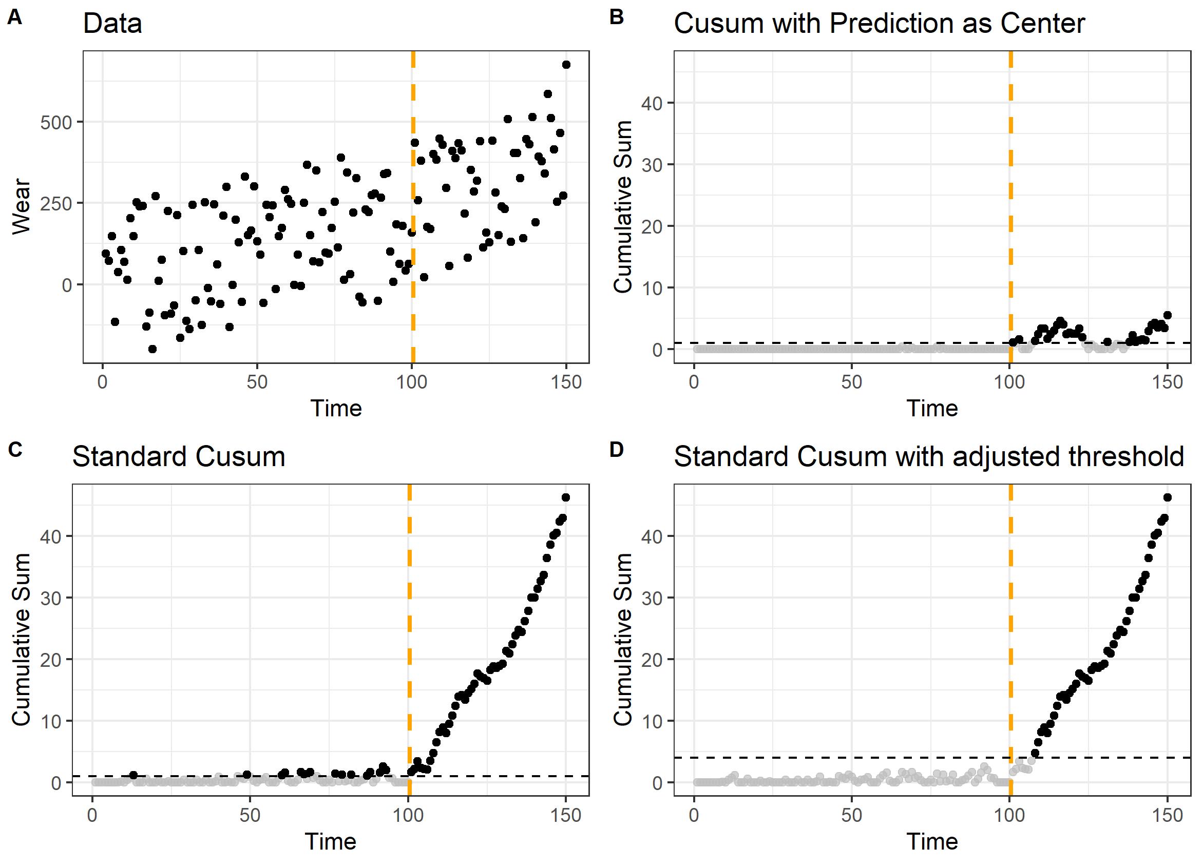
Figure 9: Part A shows some generated data with a change point at 101. Part B,C and D show results using the CUSUM method with different thresholds and $\theta$. Part B using a prediction as $\theta$ and parts C and D the standard $\theta$ of CUSUM. The thresholds of part B and C are the same and the threshold of D is higher. The black dots in part B-D represent those time when a change is detected by CUSUM. The grey dots represent those times when no changes is picked up by CUSUM. The horizontal dashed line is the threshold (in part B-D). The vertical orange line in all the plots visualizes the real change point.

4.4 Parameter

In Section 3.3 we discuss the different parameters used for our tests. Here we share our observations on how different parameter values influence the quality metrics ArlP and Fpc.

ARIMA CUSUM, CUSUM and Bayesian share a commonality: each has one parameter to consider. The impact of varying $desInt$ values on ArlP and Fpc quality measures for CUSUMis illustrated in Figure 10, revealing a divergent evolution of ArlP and Fpc. Specifically, as $desInt$ increases, Fpc exhibits a declining trend, whereas ArlP displays an ascending pattern. Since the parameter $desInt$ in ARIMA CUSUM originates from the CUSUM part, the observable behavior is the same. While the parameter of Bayesian differs from that of CUSUM ($desInt$), there is an observable trend where Fpc decreases with higher $cpthreshold$, while ArlP increases with the same increasing $cpthreshold$. OCD involves the consideration of two thresholds; however, due to the one-dimensional nature of our data, opting for a sufficiently high value for one threshold renders the influence on the outcome primarily on the other threshold. Consequently, the parallels with CUSUM emerge, as the latter method operates with a solitary threshold.

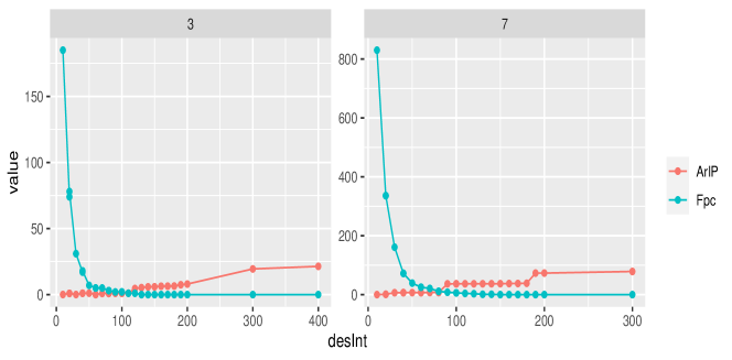
Figure 10: Each plot represents the development of ArlP and Fpc over different $desInt$ values for a certain dataset.

For LSTM CUSUM and BFAST, it is a bit more challenging to determine which parameter values will lead to which result as there are more than one parameter to consider. LSTM CUSUM has three parameters $nh$, $nz$ and $desInt$, which influence the Fpc an ArlP. If the $nz$ decreases, the Fpc decreases as well. An increase in the $nh$ parameter leads to a slight increase in the Fpc. To get a low Fpc value over multiple datasets, the middle range of the $nz$ and $nh$ parameters performed the best. The $desInt$ behaves similar to the $desInt$ in CUSUM and ARIMA CUSUM and should be chosen as small as possible to reduce the amount of Fpc.

For our experiments we used 4 different parameters for BFAST ($minHist$, $histFact$, $h$ and $level$). First, looking at each parameter separately, one can observe that the Fpc decreases with increasing $minHist$ and $h$. For $histFact$ and $level$ the opposite can be observed, with an increase in the parameter value the Fpc increases also. For ArlP the opposite is the case, low values for $minHist$ and $h$ lead to a low ArlP and high values to a high ArlP. Hence, low values for $histFact$ and $level$ lead to a high ArlP and high values to a low ArlP. These effects can still be observed by looking at the combinations of those different values.

In general, it shows that the well understood CUSUM rule with its strong control of small type I error probabilities used in the comparison step of P&C is key for the goal of strong robustness against outliers followed here. Here, a different application, where the detection of a specific type of change point is more important than few false positives may call for a different method in the comparison step.

5 Conclusion

To answer question Q3 and mention the conclusions which directly refer to the experiment, first, we report that Predict & Compare performs mostly better than the references change point detection methods. Looking at the best results for each data set (Table 3) LSTM CUSUM (data set 2,3,5 and 7) and BFAST (data set 1) are the best methods found by our experiments. The difference between the data set 2,3,5 and 7 and the data set 1 is the kind of divergent wear. The divergent wear part in data set 1 is characterised by a very short and steep slope in contrast the divergent wear in the other data set develops over a longer time period. The best method with a specific parameter set over all data sets is ARIMA CUSUM. Therefore, the ARIMA CUSUM approach is more generalized than the LSTM CUSUM approach. But ARIMA CUSUM takes longer until the change point is detected compared to LSTM CUSUM. Hence, in case of very similar data LSTM CUSUM is better in case of more diverse data ARIMA CUSUM is better. Therefore, we can - not surprisingly - conclude that a wider scope of applicability of the P&C defined CPD detectors come at the expense of sophistication of the allowed intermediate trends.

A more general observation about how well non-trivial trends occurring before change points are successfully recognized as such (and not mistaken with change points) can be drawn from Table 5 (concerning the change point from the run-in into the steady-state wear regime): It is usually ARIMA CUSUM or LSTM CUSUM which are or rank among the best methods and often beat CUSUM in terms of the time until detection. The reason for this well documented in Figure 9, which shows that CUSUM only performs comparably to CUSUM LSTM in terms of false positives, if the threshold is tuned upwards so much that longer time until detection emerges typically. The predictive model recognizes the curved trend of the run-in phase, predicts its continuation and the emerging discrepancy with the linear trend of the steady-state wear regime in the comparison step.

We conclude that in accordance with our goals, Predict & Compare provides a framework for the definition of (A) online change point detectors, which (B) allow detecting gradual structural changes and (C) cope with trends that are not to be identified as change points. While the specific two predictive models used here in the prediction part of P&C (ARIMA, LSTM) are archaic and particularly suggestive of the tribological example, they by no means spans the whole range of possible choice. Data $X_{t}$ of type (6) referring to independent numbers of specific events occurring in time intervals with an intensity that changes slowly in time (as required by goal B), the process has P&C change points (Def. 2). Data with a richer auto-correlation structure may require a much longer predictive window size. Similarly, the CUSUM rule is not the only thinkable comparison method between predicted and real values - especially if it is not the fluctuations around a trend which are the most relevant criterion for the comparison step. Thus, our demonstration of the effectiveness of P&C in comparison with other state of the art online CPD methods only shows a few of a wide variety of other potentially ideal application scenarios.

Acknowledgements

This work was funded by the Austrian COMET-Program (Project K2 InTribology1, no. 872176), and and carried out at the Software Competence Center Hagenberg.

Conflicts of interest

The authors have no conflicts of interest to declare that are relevant to the content of this article.

Data availability statement

The data that support the findings of this study are available from AC²T but restrictions apply to the availability of these data, which were used under licence for the current study, and so are not publicly available. Data are however available from the authors upon reasonable request and with permission of AC²T.

References

- \bibcommenthead
- (1) Lai, T.L.: Sequential change point detection in quality control and dynamic systems. J. Roy. Statist. Assoc. (B) 57, 613–658 (1995)
- (2) Wu, Y.: Inference for Change Point and Post Change Means After a CUSUM Test (Lecture Notes in Statistics), 1st edn. Springer, Heidelberg (2005). libgen.li/file.php?md5=72cfc291e96b7964b563672759bc9085
- (3) Pons, O.: Estimations and Tests in Change-Point Models. World Scientific Publishing Co. Pte Ltd., London (2018). https://doi.org/10.1142/10757. https://www.worldscientific.com/doi/abs/10.1142/10757
- (4) Page, E.S.: Continuous Inspection Schemes. Biometrika 41(1/2), 100 (1954). https://doi.org/10.2307/2333009. Accessed 2021-05-25
- (5) Wald, A., Wolfowitz, J.: Optimum Character of the Sequential Probability Ratio Test. The Annals of Mathematical Statistics 19(3), 326–339 (1948)
- (6) Lorden, G.: Procedures for reacting to a change in distribution. The Annals of Statistics 5 (1977)
- (7) Moustakides, G.V.: Optimality of the cusum procedure in continuous time. The Annals of Statistics 2004-feb vol. 32 iss. 1 32 (2004). https://doi.org/10.2307/3448511
- (8) Ritov, Y.: Decision theoretic optimality of the cusum procedure. The Annals of Statistics 1990-sep vol. 18 iss. 3 18 (1990). https://doi.org/10.1214/aos/1176347761
- (9) Aue, A., Horváth, L.: Structural breaks in time series. Journal of Time Series Analysis 2012-sep 14 vol. 34 iss. 1 34 (2012). https://doi.org/10.1111/j.1467-9892.2012.00819.x
- (10) Yang, P., Dumont, G., Ansermino, J.M.: Adaptive change detection in heart rate trend monitoring in anesthetized children. IEEE Transactions on Biomedical Engineering 53, 2211–2219 (2006). https://doi.org/10.1109/tbme.2006.877107
- (11) Harrison, P.J., Davies, O.L.: The use of cumulative sum (cusum) techniques for the control of routine forecasts of product demand. Operations Research 12, 325–333 (1964). https://doi.org/10.1287/opre.12.2.325
- (12) Manner, H., Stark, F., Wied, D.: Testing for structural breaks in factor copula models. Journal of Econometrics, 0304407618301842 (2018). https://doi.org/10.1016/j.jeconom.2018.10.001
- (13) Burg, G.J.J.v.d., Williams, C.K.I.: An Evaluation of Change Point Detection Algorithms. arXiv:2003.06222 [cs, stat] (2020). arXiv: 2003.06222. Accessed 2022-01-14
- (14) Aminikhanghahi, D.J. Samaneh; Cook: A survey of methods for time series change point detection. Knowledge and Information Systems 2016-sep 08 vol. 51 iss. 2 51 (2016). https://doi.org/10.1007/s10115-016-0987-z
- (15) Siegmund, D.: Sequential Analysis. Springer, Heidelberg (1985)
- (16) Truong, C., Oudre, L., Vayatis, N.: Selective review of offline change point detection methods. Signal Processing 2020-feb vol. 167 167 (2020). https://doi.org/10.1016/j.sigpro.2019.107299
- (17) Cao, Y., Xie, L., Xie, Y., Xu, H.: Sequential change-point detection via online convex optimization. Entropy 2018-feb 07 vol. 20 iss. 2 20 (2018). https://doi.org/10.3390/e20020108
- (18) Hawkins, D.M., Olwell, D.H.: Cumulative Sum Charts and Charting for Quality Improvement. Springer, New York, NY (1998). https://doi.org/10.1007/978-1-4612-1686-5. http://link.springer.com/10.1007/978-1-4612-1686-5 Accessed 2021-05-25
- (19) Abdul Halim Lim, S., Antony, J., Arshed, N., Albliwi, S.: A systematic review of statistical process control implementation in the food manufacturing industry. Total Quality Management & Business Excellence, 1–14 (2015). https://doi.org/10.1080/14783363.2015.1050181
- (20) Ma, Q., Zheng, Y., Yang, W., Zhang, Y., Zhang, H.: Remaining useful life prediction of lithium battery based on capacity regeneration point detection. Energy 234, 121233 (2021). https://doi.org/10.1016/j.energy.2021.121233
- (21) Montgomery, D.C.: Statistical Quality Control, 7th edn. Wiley, Hoboken, New Jersey (2012)
- (22) Bücher, A., Dette, H., Heinrichs, F.: Are deviations in a gradually varying mean relevant? A testing approach based on sup-norm estimators (2020)
- (23) Vogt, M., Dette, H.: Detecting gradual changes in locally stationary processes. The Annals of Statistics 43, 713–740 (2015). https://doi.org/10.1214/14-aos1297
- (24) Aue, A., Steinebach, J.: A note on estimating the change-point of a gradually changing stochastic process. Statistics & Probability Letters 56, 177–191 (2002). https://doi.org/10.1016/s0167-7152(01)00184-5
- (25) Woodall, W.H., Adams, B.M.: The statistical design of cusum charts. Quality Engineering 5(4), 559–570 (1993). https://doi.org/10.1080/08982119308918998. Accessed 2021-05-25
- (26) Bissell, A.F.: The performance of control charts and cusums under linear trend. Journal of the Royal Statistical Society: Series C (Applied Statistics) 33, 145–151 (1984). https://doi.org/10.2307/2347439
- (27) Verbesselt, J., Hyndman, R., Newnham, G., Culvenor, D.: Detecting trend and seasonal changes in satellite image time series. Remote Sensing of Environment 114(1), 106–115 (2010). https://doi.org/10.1016/j.rse.2009.08.014
- (28) Ryan Prescott Adams, D.J.C.M.: Bayesian online changepoint detection (2007)
- (29) Chen, Y., Wang, T., Samworth, R.J.: High-Dimensional, Multiscale Online Changepoint Detection. Journal of the Royal Statistical Society Series B: Statistical Methodology 84(1), 234–266 (2022). https://doi.org/10.1111/rssb.12447
- (30) Agudelo-España, D., Gomez-Gonzalez, S., Bauer, S., Schölkopf, B., Peters, J.: Bayesian Online Prediction of Change Points. arXiv:1902.04524 [cs, stat] (2020). arXiv: 1902.04524. Accessed 2022-05-09
- (31) Wang, Z., Lin, X., Mishra, A., Sriharsha, R.: Online changepoint detection on a budget. In: 2021 International Conference on Data Mining Workshops (ICDMW), pp. 414–420. IEEE Computer Society, Los Alamitos, CA, USA (2021). https://doi.org/10.1109/ICDMW53433.2021.00057. https://doi.ieeecomputersociety.org/10.1109/ICDMW53433.2021.00057
- (32) Gardner, E.S., Mckenzie, E.: Forecasting Trends in Time Series. Management Science 31(10), 1237–1246 (1985). https://doi.org/10.1287/mnsc.31.10.1237. Accessed 2023-08-17
- (33) Krause, M.: Unsupervised change point detection for heterogeneous sensor signals (2023). arXiv:2305.11976v1
- (34) Yu, H., Liu, T., Lu, J., Zhang, G.: Automatic Learning to Detect Concept Drift. arXiv (2021). https://doi.org/10.48550/ARXIV.2105.01419. https://arxiv.org/abs/2105.01419
- (35) De Brabandere, A., Cao, Z., De Vos, M., Bertrand, A., Davis, J.: Semi-supervised change point detection using active learning. In: Discovery Science: 25th International Conference, DS 2022, Montpellier, France, October 10–12, 2022, Proceedings, pp. 74–88. Springer, Berlin, Heidelberg (2022). https://doi.org/10.1007/978-3-031-18840-4_6. https://doi.org/10.1007/978-3-031-18840-4_6
- (36) Liu, P.F.Z.: On-line inference for multiple changepoint problems. Journal Of The Royal Statistical Society 69, 589–605 (2007). https://doi.org/10.1111/j.1467-9868.2007.00601.x
- (37) Agudelo-España, D., Gomez-Gonzalez, S., Bauer, S., Schölkopf, B., Peters, J.: Bayesian Online Prediction of Change Points. arXiv:1902.04524 [cs, stat] (2020). arXiv: 1902.04524. Accessed 2022-05-09
- (38) Malladi, R., Kalamangalam, G.P., Aazhang, B.: Online Bayesian change point detection algorithms for segmentation of epileptic activity. In: 2013 Asilomar Conference on Signals, Systems and Computers, pp. 1833–1837. IEEE, Pacific Grove, CA, USA (2013). https://doi.org/10.1109/ACSSC.2013.6810619. http://ieeexplore.ieee.org/document/6810619/ Accessed 2023-08-29
- (39) Lau, H.F., Yamamoto, S.: Bayesian online changepoint detection to improve transparency in human-machine interaction systems. In: 49th IEEE Conference on Decision and Control (CDC), pp. 3572–3577. IEEE, Atlanta, GA, USA (2010). https://doi.org/10.1109/CDC.2010.5717959. http://ieeexplore.ieee.org/document/5717959/ Accessed 2023-08-29
- (40) van Houwelingen; Joseph G. Ibrahim; Thomas H. Scheike, J.P.K.H.C.: Handbook of Survival Analysis. Chapman & Hall / CRC Handbooks of Modern Statistical Methods. Chapman and Hall/CRC, Boca Raton, FL (2013). ISBN=978-1-4665-5567-9,978-1-4665-5566-2
- (41) Verbesselt, J., Zeileis, A., Herold, M.: Near real-time disturbance detection using satellite image time series. Remote Sensing of Environment 123, 98–108 (2012). https://doi.org/10.1016/j.rse.2012.02.022. Accessed 2022-03-28
- (42) Sharma, S., Swayne, D.A., Obimbo, C.: Trend analysis and change point techniques: a survey. Energy, Ecology and Environment 1(3), 123–130 (2016). https://doi.org/10.1007/s40974-016-0011-1. Accessed 2022-05-08
- (43) Basseville, M., Nikiforov, I.: Fault isolation for diagnosis: nuisance rejection and multiple hypotheses testing. Annual Reviews in Control, 14 (2002)
- (44) Bissell, A.F.: Cusum techniques for quality control (with discussion). Applied Statistics 18, 1–30 (1969)
- (45) Chang, T.C., Gan, F.F.: A cumulative sum control chart for monitoring process variance. Journal of Quality Technology 27(2), 109–119 (1995) https://doi.org/10.1080/00224065.1995.11979574. https://doi.org/10.1080/00224065.1995.11979574
- (46) Jech, M., Lenauer, C.: Radionuclide methods. In: Friction, Lubrication, and Wear Technology. ASM Handbook, vol. 18, pp. 1045–1055. ASM International, Ohio, USA (2017)
- (47) Glock, A.-C., Sobieczky, F., Jech, M.: Detection of anomalous events in the wear-behaviour of continuously recorded sliding friction pairs. Conference Proceedings ÖTG-Tagung 2019, 30–40 (2019). ISBN:9783901657627
- (48) Feller, W.: Probability Theory vol. II. Wiley, Hoboken, New Jersey (2019). Chap. VI.6
- (49) Zeileis, A., Leisch, F., Kleiber, C., Hornik, K.: Monitoring structural change in dynamic econometric models. Journal of Applied Econometrics 20(1), 99–121 (2005). https://doi.org/10.1002/jae.776. Accessed 2022-10-12
- (50) Brisset, P., Ditroi, F., Eberle, D., Jech, M., Kleinrahm, A., Lenauer, C., Sauvage, T., Thereska, J.: Radiotracer Technologies for Wear, Erosion and Corrosion Measurement. TECDOC Series, vol. 1897. International Atomic Energy Agency, Vienna (2020). Chap. 5.5.3
- (51) Scrucca, L.: qcc: an r package for quality control charting and statistical process control. R News 4/1, 11–17 (2004)
- (52) Hyndman, R.J., Khandakar, Y.: Automatic time series forecasting: the forecast package for R. Journal of Statistical Software 26(3), 1–22 (2008). https://doi.org/10.18637/jss.v027.i03
- (53) Hyndman, R., Athanasopoulos, G., Bergmeir, C., Caceres, G., Chhay, L., O’Hara-Wild, M., Petropoulos, F., Razbash, S., Wang, E., Yasmeen, F.: forecast: Forecasting Functions for Time Series and Linear Models. (2022). R package version 8.16. https://pkg.robjhyndman.com/forecast/
- (54) Chollet, F., Allaire, J., et al.: R Interface to Keras. GitHub (2017)
- (55) Hinkley, D.V.: Inference about the change-point in a sequence of random variables. Biometrika 57, 1–17 (1970). https://doi.org/10.2307/2334932