On the Dynamical Hierarchy in Gathering Protocols with Circulant Topologies

Abstract

In this article we investigate the convergence behavior of gathering protocols with fixed circulant topologies using tools form dynamical systems. Given a fixed number of mobile entities moving in the Euclidean plane, we model a gathering protocol as a system of ordinary differential equations whose equilibria are exactly all possible gathering points. Then, we find necessary and sufficient conditions for the structure of the underlying interaction graph such that the protocol is stable and converging, i.e., gathering, in the distributive computing sense by using tools from dynamical systems. Moreover, these tools allow for a more fine grained analysis in terms of speed of convergence in the dynamical systems sense. In fact, we derive a decomposition of the state space into stable invariant subspaces with different convergence rates. In particular, this decomposition is identical for every (linear) circulant gathering protocol, whereas only the convergence rates depend on the weights in interaction graph itself.

1 Introduction

This article applies dynamical systems theory to the design and analysis of collective behavior of swarms of mobile entities, called robots from now on, which are widely studied in the computer science community under the headline of distributed computing (e.g. [Ham18, FPS12, FPS19]). Envision a scenario where a distributed system of mobile robots is supposed to establish a certain formation in the plane (more general spaces are possible but shall be neglected here). Formations under investigation vary from simple straight lines and circles to more complex structures that the robots are supposed to distribute evenly in (see e.g. [FPSV17, SY06, LC08, CP06]). The most basic formation problem, however, is the gathering problem in which the robots are supposed to gather in a single, not predefined, point.

The robots capabilities to accomplish their task are limited. Typical assumptions are that they are externally identical (every robot looks the same), anonymous (they do not have unique identifiers), and oblivious (they do not remember past steps). The only capabilities the robots have are observing other robots’ positions, performing computations in their local memory, and move. The observation of another robot’s position is a form of communication or interaction. Commonly, the robots are additionally assumed to be limited in their communication capabilities as well by having only a limited viewing range $\mathcal{C}>0$ within which they can perceive the positions of other robots. In particular, the robots do not share a common coordinate system. To reach a formation, each robot plans its movement individually according to its observations. In particular, there is no external control. The strategy that each robot pursues is called a protocol. Crucially, the protocols of all robots are identical (the robots are also identical internally).

Most protocols for formation problems are based on a discrete time model. Robots act in synchronous so-called Look-Compute-Move (LCM) rounds, consisting of the determination of the relative positions of neighbors, the computation of a target point, and the movement to that target point. This is commonly is referred to as the $\mathcal{F}$sync model. Multiple protocols to solve the gathering problem have been developed for this model (and also for more powerful robots) [ASY95, DKL⁺11, CFH⁺20, CP05, LV19, IKIW07, Flo19]. On the other hand protocols using a continuous time model are less studied. In this situation, all robots perform their LCM rounds permanently and instantaneously. The Move part is modified to the continuous adjustment of speed and direction. This continuous motion model might seem unrealistic, e.g., due to the assumption that there is no delay between the robots’ sensors and actors. However, it was pointed out that it is comparatively close to real applications. Several protocols to address the gathering problem have been proposed as well [DKKM15, KMadH19].

Typically, studies as the ones referenced above do not only prove that an introduced protocol solves the investigated problem but also analyze the collective dynamics of the robot swarm in terms of the speed with which a protocol solves a given task. This allows for the comparison of different protocols. The speed of a protocol is commonly assessed by runtime analysis of the corresponding algorithms through combinatorical investigations. It can be observed that a given protocol causes the robots in one configuration (the collective state of all robots’ positions) to gather much faster than in another (e.g., [DKL⁺11]). This can be used to derive best and worst-case runtimes.

The key contribution of this article is to show that applying the mathematical theory of dynamical systems to this problem class from distributed computing allows for a more profound understanding of the collective dynamics. In particular, it is possible to determine the final gathering point and to identify a hierarchy of gathering rates with corresponding configurations. To that end, we will focus on the gathering problem of robots with the limitations outlined above performing continuous protocols. The interaction structure between robots is assumed to be circulant (compare to Example 1.1 below) and remains unchanged throughout the dynamics. This slightly weakens the assumption of anonymity because each robot is able to identify the robots it communicates with. Furthermore, we do not make the assumption of a finite communication range in general. We will address this limitation separately on multiple occasions. For the most part, we restrict to linear protocols, i.e., each robot computes its target point as a linear combination of the positions of its neighbors. However, we outline options to generalize to nonlinear protocols as well.

As a first step, we investigate the interaction structure of the robots. We represent the fixed interactions using a weighted graph corresponding to the robots and communication channels which we call the interaction graph. Dynamical systems theory allows us to unveil necessary and sufficient conditions that this graph has to satisfy in order for a protocol to solve the gathering problem. For example, we show in Theorem 3.9 that a general linear protocol of this kind is gathering if and only if the weight matrix of the interaction graph has specific spectral properties. For a circulant protocol of this kind the result simplifies to the condition that the interaction graph is connected and the weights sum to $1$ (see Theorem 3.16).

Focusing on linear protocols with a circulant interaction graph, we then perform a more fine grained analysis of the dynamics. In particular, we unveil a foliation of the state space of all robots’ positions into dynamically invariant subspaces in which the configurations gather with different speeds. This foliation is independent of the precise protocol. It allows to identify gathering rates for different initial configurations (cf. Theorem 4.4) and to decompose initial configurations into components with different gathering rates (cf. Corollary 4.6).

We would like to point out the reference [KMadH11] which largely inspired the work on this project. Therein the authors apply the theory of Markov chains to robots forming a chain between two fixed stations in a discrete time model under a similarly rigid interaction structure. In [Kli10], one of the authors takes a brief outlook on how to extend these methods to the gathering problem. This has thoroughly been analysed in [CHJ⁺23] for a different class of algorithms. While the mathematical investigation in [KMadH11] bears some semblances to the one in this article, the different setup requires entirely different proofs.

Before we dive into the details of modelling the gathering problem as a dynamical system and analyzing it for collective dynamics, we illustrate the main results at the hand of the following example.

Example 1.1.

Consider $N=7$ mobile robots that we identify with their indices $\left\{\,0,\dotsc,6\,\right\}$. The robots are running the Go-To-The-Middle protocol. That is, if $z_{i}(t)\in\mathbb{R}^{2}$ is the position of robot $i$ at time $t$ the $i$-th robot will move towards the midpoint between its two neighbors

$$\frac{1}{2}\left(z_{i-1}(t)+z_{i+1}(t)\right),$$

where we require the convention that $z_{-1}=z_{6}$ and $z_{7}=z_{0}$. In particular, each robot communicates with its left and right neighbors when arranged on a circle. Theorem 3.16 shows that this is indeed a dynamical systems model of a protocol that solves the gathering problem. Furthermore, Figure 1 displays two different initial configurations. Applying Theorem 4.4 shows that the configuration on the left in (a) has the slowest gathering rate, while the configuration on the right in (b) has the fastest gathering rate. Further intermediate configurations are unveiled as well. The details will be developed below.

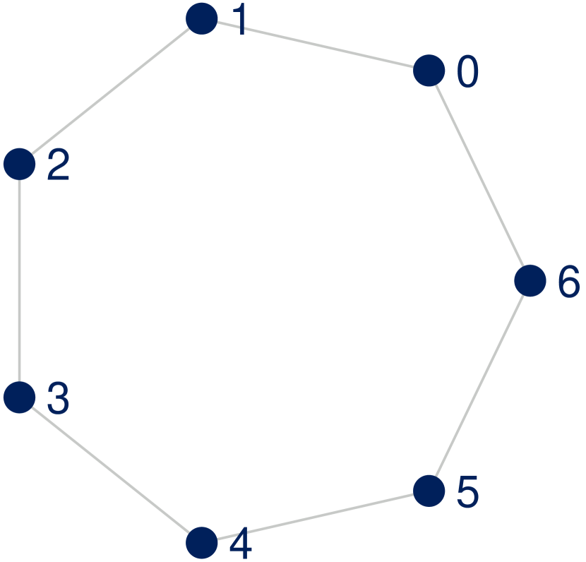
(a) Slowly gathering configuration

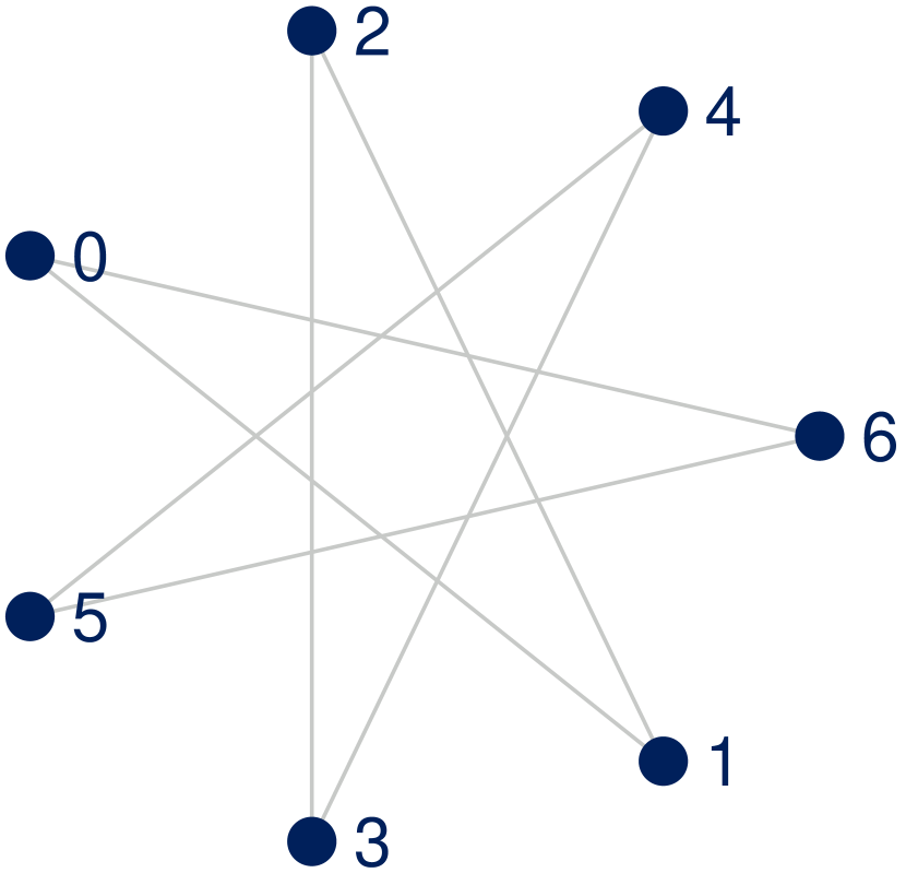
(b) Fast gathering configuration

Figure 1: Illustration of the gathering hierarchy exhibited by $N=7$ robots running the Go-To-The-Middle protocol. Blue dots indicate positions of each robot. Gray lines symbolize the communication relation. The configuration in (a) corresponds to the slowest gathering rate. The configuration (b) corresponds to the fastest gathering rate.

The article is organized as follows: In Section 2 we introduce the general problem. This contains Section 2.1 in which we introduce necessary notation and model the problem as a dynamical system governed by an ordinary differential equation. In Section 2.2, we introduce circulant interaction graphs. Section 3 contains the investigation of general gathering protocols. We argue why it is reasonable to focus on linear systems (Section 3.2) and deduce conditions for gathering both for general (Section 3.3) and for circulant systems (Section 3.4). Some of the more technical proofs are postponed to Appendix A. Finally, in Section 4, we develop the main dynamical analysis by proving the hierarchy of different gathering rates.

Acknowledgements

The authors would like to express their special gratitude to Friedhelm Meyer auf der Heide, Jannik Castenow, and Jonas Harbig who provided invaluable inspiration and counsel for the distributed computing side of the project and took part in the development of some of the research ideas presented in this manuscript in numerous spirited and productive discussions. This work is funded by the Deutsche Forschungsgemeinschaft (DFG, German Research Foundation) – Project number 453112019.

2 Introductory Considerations

2.1 Notations and Definitions

We begin by setting up a dynamical systems model for the collective dynamics of a collection of $N\in\mathbb{N}$ interacting mobile robots. For simplicity of notation, we refer to individual robots only by their label according to an arbitrarily chosen enumeration, i.e., $\left\{\,0,\dotsc,N-1\,\right\}$ is the set of robots. The robots move in the Euclidean plane in continuous time and we denote the position of robot $i\in\left\{\,0,\dotsc,N-1\,\right\}$ at time $t\in\mathbb{R}$ by $z_{i}(t)=(x_{i}(t),y_{i}(t))\in\mathbb{R}^{2}$. The collection of all robots’ positions is called a configuration. As mentioned above, each robot observes the positions of (a subset of) the other robots in relative coordinates. However, we take the stance of an external observer describing the dynamics in global coordinates. Each robot then adapts its own direction and speed of movement instantaneously as in a Look-Compute-Move cycle (LCM) in continous time. We model this instantaneous adaptation by a system of ordinary differential equations (ODEs) of the form

$$\dot{z_{i}}(t)=-z_{i}(t)+f(z_{0}(t),\dotsc,z_{N-1}(t)),\quad i=0,\dotsc,N-1.$$ (1)

The collection of all equations (1) models the movement of all robots $i\in\left\{\,0,\dotsc,N-1\,\right\}$. Here, $\dot{z_{i}}(t)$ denotes the derivative of $z_{i}(t)$ with respect to time $t\in\mathbb{R}$. In particular, the left hand side of (1) is the velocity vector of the $i$-th robot. The function $f:\mathbb{R}^{2N}\to\mathbb{R}^{2}$ describes which target point the robot computes according to the positions of its neighboring robots given by $z_{0}(t),\dotsc,z_{N-1}(t)$. Hence, by subtracting its own current position $z_{i}(t)$ the left hand side of (1) models the movement to that target point $f(z_{0}(t),\dotsc,z_{N-1}(t))$. The system (1) is autonomous since $f$ does not depend on time $t\in\mathbb{R}$. Note that, in general, not every neighboring position $z_{j}(t)$ will influence the dynamics of the $i$-th robot, i.e., its dynamics is in fact independent of $z_{j}(t)$ for some $j\in\left\{\,0,\dotsc,N-1\,\right\}$. We will go into the details of the topology of of these interactions below. We assume $f$ to be at least continuously differentiable, which ensures existence and uniqueness of solutions $z_{i}(t)$ for a prescribed initial point and also allows us to apply classical tools from dynamical systems theory. Moreover, we emphasize that the robots are identical and as such all of them react to their neighbors positions in exactly the same way. This is reflected by the fact that the function governing the right hand side $f$ of (1) is the same for every robot $i$. Finally, note that we will frequently omit the time argument in the presentation when time $t$ is clear from context or its precise value is not important. This convention is common in the dynamical systems literature and allows us to simplify notation, for example by writing $z_{i}$ instead of $z_{i}(t)$.

Since we are modeling a gathering protocol, we assume that every robot is at rest, when all robots share the same position $z_{i}=z^{*}=(x^{*},y^{*})\in\mathbb{R}^{2}$ for all $i\in\left\{\,0,\dotsc,N-1\,\right\}$, which will be called a gathering point. Note that we do not assume uniqueness of this position, as the gathering point is independently determined by the robots and it is not predefined. In terms of the ODE model (1) this means that $\dot{z}_{i}=0$, if and only if $z_{i}=z^{*}$ for all $i\in\left\{\,0,\dotsc,N-1\,\right\}$. That is, the system has to be in equilibrium for any such configuration. In particular, this implies that the right hand side has to vanish meaning

$$f(z^{*},\dotsc,z^{*})=z^{*}\text{ for all }z^{*}\in\mathbb{R}^{2}.$$ (2)

In the distributed computing literature any such protocol satisfying this assumption is said to be stable [HJPR87, SS94].

Remark 2.1.

In general, in the distributed computing sense the term ’stable’ refers to a property that once true on a state, it remains true forever [SS94]. Translating this definition for the ODE model (1) precisely yields (2), i.e., every gathering point is an equilibrium of (1). Note that, there is also the definition of stability for an equilibrium in the dynamical systems sense: An equilibrium $z^{*}$ is said to be stable if every trajectory initialized sufficiently close to $z^{*}$ stays close to $z^{*}$ for all times. We highlight that both definitions, though slightly related, have a different meaning which is due to their origin in the distributed computing, respectively dynamical systems community. On the one had stability is a property of a protocol or model, and on the other hand it is a property of an equilibrium, e.g., a gathering point in our setting.

Collecting every position $z_{i}=(x_{i},y_{i})\in\mathbb{R}^{2}$ of each robot $i$ in a single vector defined by $Z(t)=(z_{0}(t),\dotsc,z_{N-1}(t))=(x_{0}(t),y_{0}(t),\dotsc,x_{N-1}(t),y_{N-1}(t))\in\mathbb{R}^{2N}$, allows us to write the system of all equations (1) as

$$\dot{Z}(t)=F(Z(t))=-Z(t)+\begin{pmatrix}f(Z(t))\\ \vdots\\ f(Z(t))\end{pmatrix},$$ (3)

i.e., $F:\mathbb{R}^{2N}\to\mathbb{R}^{2N}$ is constructed by stacking all equations (1) in a single function. Note that (3) has a steady state $Z^{*}\in\mathbb{R}^{2N}$, which is by construction of the form $Z^{*}=(z^{*},z^{*},\dotsc,z^{*})\in\mathbb{R}^{2N}$ and thus will be called synchronous state. We define the subspace of all synchronous states by $\operatorname{Syn}=\left\{\,Z^{*}=(z^{*},\dotsc,z^{*})\ \vrule\ z^{*}\in\mathbb{R}^{2}\,\right\}\subseteq\mathbb{R}^{2N}$.

In some cases, it turns out to be helpful to arrange the coordinates of all robots’ positions into a single vector in another way, which is $\widetilde{Z}:=(X,Y)\in\mathbb{R}^{2N}$, where $X=(x_{0},\dotsc,x_{N-1})\in\mathbb{R}^{N}$ denotes the $x$-coordinates of the $N$ robots and $Y=(y_{0},\dotsc,y_{N-1})\in\mathbb{R}^{N}$ the $y$-coordinates, respectively. In these coordinates the corresponding synchronous state is $\widetilde{Z}^{*}=(X^{*},Y^{*})=(x^{*},\dotsc,x^{*},y^{*},\dotsc,y^{*})\in\mathbb{R}^{2N}$. We note that this particular order will be useful for the upcoming dynamical analysis.

Typically, one encodes the pairwise interactions between robots by a graph $G=(V,E)$. Here, the vertices are the robots $V=\left\{\,0,\dotsc,N-1\,\right\}$ and an edge $e=(j,i)\in E\subseteq V\times V$ represents the fact that robot $i$ adapts its movement using the position of robot $j$. In other terms, an edge represents the fact that robot $j$ influences robot $i$. On the other hand, if the edge $e=(j,i)$ is not in $E$ then robot $j$ has no impact on the movement of robot $i$. We refer to this graph as the interaction graph. It is common and useful to further encode the graph structure in terms of an adjacency matrix of the form

$$\begin{split}A=(a_{i,j})_{i,j=0}^{N-1}\in\left\{\,0,1\,\right\}^{N\times N},a_{i,j}=\begin{cases}1,\text{ if $e=(j,i)\in E$, i.e, robot $j$ influences robot $i$,}\\ 0,\text{ otherwise.}\end{cases}\end{split}$$

By construction we can read off all robots $j$ that influence robot $i$ in the $i$-th row of $A$.

In this article, we will focus on the situation that the interaction structure is fixed for all times, that is, the subset of robots that $i$ uses to compute its velocity vector remains unchanged no matter what position these robots are in. In particular, this means that no connections are added or removed from $E$ as time proceeds and there is no limited viewing range. Moreover, we assume the interaction graph to be weighted, that is, each edge $e=(j,i)\in E$ is assigned a weight $w_{i,j}\in\mathbb{R}\setminus\left\{\,0\,\right\}$. These allow each robot to distinguish between its influences. We assemble the so-called weight matrix $W=(w_{i,j})_{i,j=0}^{N-1}\in\mathbb{R}^{N\times N}$, where we set $w_{i,j}=0$ if $e=(j,i)\notin E$. Note that $w_{i,j}=0$ if and only if $a_{i,j}=0$ by construction.

In the remainder of this article, we will further refer to and exploit several structural properties that the interaction graph $G$ – and as a result also $A$ - may or may not have. In particular, the interaction graph is called connected (or weakly connected) if for any two vertices $j,i\in\left\{\,0,\dotsc,N-1\,\right\}$ there is an undirected path from $j$ to $i$, i.e., there are vertices $k_{0}=j,k_{1},\dotsc,k_{l+1}=i\in\left\{\,0,\dotsc,N-1\,\right\}$ such that $(k_{r-1},k_{r})\in E$ or $(k_{r},k_{r-1})\in E$ for $r=1,\dotsc,l+1$. It is called strongly connected if for any two vertices $j,i\in\left\{\,0,\dotsc,N-1\,\right\}$ there is a directed path from $j$ to $i$, i.e. there are vertices $k_{0}=j,k_{1},\dotsc,k_{l+1}=i\in\left\{\,0,\dotsc,N-1\,\right\}$ such that $(k_{r-1},k_{r})\in E$ for $r=1,\dotsc,l+1$. It is clear that strong connectivity implies weak connectivity. Note that the connectivity of an interaction graph does not depend on the weights assigned to each edge. Finally, any weight matrix $W\in\mathbb{R}^{N\times N}$ corresponding to a strongly connected graph is called irreducible.

Using the interaction graph, we can adapt the robot’s individual dynamics in (1) to reflect the interaction structure and consider

$$\dot{z_{i}}=-z_{i}+f(z_{I(i)}),$$

where $z_{I(i)}$ represents the collection of positions of those robots that $i$ actually uses to adapt its own movement (note the abuse of notation in the function $f$). More precisely, $I(i):=\left(j\ \vrule\ e=(j,i)\in E\right)=\left(j\ \vrule\ a_{i,j}=1\right)$ denote the (ordered) tuple of robots $j$ that influence the dynamics of robot $i$ and

$$z_{I(i)}=(z_{j}\ \vrule\ j\in I(i))$$

is defined as the corresponding neighboring positions. Since the robots in our model are able to distinguish between each other, the precise order in which the arguments enter $f$ matters. Hence, $I(i)$ and $z_{I(i)}$ are assumed to be (ordered) tuples rather than sets. Their explicit order corresponds to the interaction topology that we specify below.

Finally, we introduce some terminology regarding properties of a protocol modeled by (1). It is analogous to that used in [KMadH11].

Definition 2.2.

A protocol modeled by (1) is called convergent, if the solution with any initial configuration converges to a gathering point for $t\to\infty$. It is called gathering if it is both stable (cf. (2)) and convergent.

Remark 2.3.

1. Although similar, the notions are not equivalent, as neither implies the other. For example, consider (1) with $f(Z)=0$. Then one readily sees that the solution for any initial configuration converges to $\overline{Z}=(0,\dotsc,0)^{T}\in\mathbb{R}^{2N}$. While this is indeed a gathering point, it also implies that any gathering initial condition $Z^{*}\neq(0,\dotsc,0)\in\mathbb{R}^{2N}$ also converges. In particular, the system is not in equilibrium at $Z^{*}\in\mathbb{R}^{2N}$. Thus, the protocol is convergent but not stable.

2. As the definition of ’convergent’ for a protocol addresses convergence of initial points to a gathering point, i.e, an equilibrium for a stable protocol, it can arguably be related to the notion of asymptotic stability in the dynamical systems sense. An equilibrium is called asymptotic stable, if it is stable and every initial point sufficiently close to the equilibrium converges to it. Again, with Remark 2.1 in mind, both notions are related, although they have a different meaning.

3. Note that, the notion of ’convergent’ does not include any characterization of the speed or rate of convergence. We will address this issue later in Section 4.

2.2 Circulant Topology

The focus of this article lies in the dynamical analysis of (3) with a circulant interaction topology. This is best illustrated by an example as in Figure 2, where vertices of the interaction graph are arranged in a circle and labelled accordingly.

Figure 2: Illustration of an interaction graph with circulant topology. Each vertex is influenced by its second neighbor on the left and its first neighbor on the right.

We deliberately refer to vertices instead of robots, as the illustration does not correspond to the physical locations of the individual robots but only illustrates the structure of their interactions. Vertex $i$ is influenced by its $k$-th neighbor to the left/right in the circle if and only if all of the robots are influenced by their $k$-th neighbor to the left/right and all of them react to that neighbors’ position in the same way. In particular, the interaction graph is circulant if and only if there are integers $0\leq s_{1}<\dotsb<s_{k}\leq N-1$ – sometimes referred to as jumps – such that

$$I(i)=(i+s_{1}\bmod N,\dotsc,i+s_{k}\bmod N)$$

Note that this fixes the order of $I(i)$ to be increasing $\bmod\,N$ starting from $i$.

This prescribed circulant interaction structure implies a certain structure of its adjacency matrix $A\in\left\{\,0,1\,\right\}^{N\times N}$ and weight matrix $W\in\mathbb{R}^{N\times N}$, i.e., both are circulant matrices defined by

$$\begin{split}A&=\operatorname{circ}(a_{0},a_{1},\dotsc,a_{N-1}):=\begin{pmatrix}a_{0}&a_{1}&\cdots&a_{N-2}&a_{N-1}\\ a_{N-1}&a_{0}&a_{1}&&a_{N-2}\\ \vdots&a_{N-1}&a_{0}&\ddots&\vdots\\ a_{2}&&\ddots&\ddots&a_{1}\\ a_{1}&a_{2}&\cdots&a_{N-1}&a_{0}\end{pmatrix}\in\left\{\,0,1\,\right\}^{N\times N},\\[10.00002pt] W&=\operatorname{circ}(w_{0},w_{1},\dotsc,w_{N-1}):=\begin{pmatrix}w_{0}&w_{1}&\cdots&w_{N-2}&w_{N-1}\\ w_{N-1}&w_{0}&w_{1}&&w_{N-2}\\ \vdots&w_{N-1}&w_{0}&\ddots&\vdots\\ w_{2}&&\ddots&\ddots&w_{1}\\ w_{1}&w_{2}&\cdots&w_{N-1}&w_{0}\end{pmatrix}\in\mathbb{R}^{N\times N}.\end{split}$$

Thus, $A$ and $W$ are fully specified by a vector $a\in\left\{\,0,1\,\right\}^{N}$ and $w\in\mathbb{R}^{N}$ respectively, which are cyclically permuted/shifted in each row. In this sense, we say $a=(a_{0},\dotsc,a_{N-1})$ ($w=(w_{0},\dotsc,w_{N-1})$) generates the circulant matrix $A$ ($W$) and therefore the underlying graph and topology. Hence, for a circulant adjacency matrix it is sufficient to specify the robots $j$ that influence the first robot. This structure can also by characterized by noting that the $(i,j)$-th entry of $A$ ($W$) is given by

$$A_{i,j}=a_{(j-i)\bmod N}\text{ resp. }W_{i,j}=w_{(j-i)\bmod N}.$$

For instance, the vector $a=(0,1,0,\dotsc,0,1,0)\in\left\{\,0,1\,\right\}^{N}$ generates the adjacency matrix

$$A=\begin{pmatrix}0&1&0&\cdots&0&1&0\\ 0&0&1&0&\cdots&0&1\\ 1&0&0&1&0&\cdots&0\\ \vdots&&\vdots&&\vdots&&\vdots\\ 0&0&0&\cdots&0&0&1\\ 1&0&0&\cdots&1&0&0\end{pmatrix},$$

which encodes the interaction graph given in Figure 2.

Example 2.4.

As a first running example we will consider the $N$-bug problem [WK69]. In this protocol each robot/vertex $i$ is only influenced by its first right neighbor, which yields a (non-symmetric) circulant interaction structure of the form $A=\operatorname{circ}(0,1,0\dotsc,0)$. Here, we only have one jump $s_{1}=1$ and in Figure 3 we illustrate its topology.

Figure 3: Illustration of the circulant interaction graph of the $N$-bug problem.

The additional symmetry that is introduced into an interaction graph by circulant interaction structure has the convenient side-effect that weak and strong connectivity are equivalent. This is due to the observation, that given an edge $e=(j,i)\in E$ one can construct a directed path from $i$ to $j$, which then replaces every edge, that has the ’wrong’ direction in an undirected path.

Lemma 2.5.

Let $G=(\left\{\,0,\dotsc,N-1\,\right\},E)$ be a circulant interaction graph determined by the jumps $0\leq s_{1}<\dotsb<s_{k}\leq N-1$. Then the following are equivalent

1. $G$ is weakly connected.

2. $G$ is strongly connected.

Proof.

By definition of both notions we only have to prove the first implication.

(i) $\implies$ (ii): Consider an arbitrary edge $(j,i)\in E$. By definition there exists $r\in\left\{\,1,\dotsc,k\,\right\}$ such that $j=i+s_{r}\bmod N$. Then also $(j+s_{r}\bmod N,j)\in E$, as well as $(j+2s_{r}\bmod N,j+s_{r}\bmod N)\in E$ and so forth. This can be continued to show that $(j+ls_{r}\bmod N,j+(l-1)s_{r}\bmod N)\in E$ for all $r\geq 1$. Their concatenation obviously constitutes a directed path. In particular, continuing until $l=N-1$, we obtain a directed path from $j+(N-1)s_{r}\bmod N$ to $j$. Since $j+(N-1)s_{r}\bmod N=i+Ns_{r}\bmod N=i$, this is a directed path from $i$ to $j$ – in addition to the directed edge from $j$ to $i$.

In conclusion, for every directed edge in the graph there exists a directed path in the opposite direction. Hence, for every undirected path from $j$ to $i$ there is also a directed path from $j$ to $i$ that we obtain by replacing all edges in the ’wrong’ direction with the directed path in the opposite direction. In particular, if the graph is assumed to be weakly connected it is strongly connected as well.

∎

While connectivity can be computed efficiently, it is occasionally useful to have a purely combinatorical condition at hand. We state the following result from graph theory without a proof.

Proposition 2.6 ([vD86, Corollary 1]).

Consider the circulant interaction graph $G=(\left\{\,0,\dotsc,N-1\,\right\},E)$ determined by the jumps $0\leq s_{1}<\dotsb s_{k}\leq N-1$. Then $G$ is connected if and only if

$$\gcd(N,s_{1},\dotsc,s_{k})=1,$$ (4)

where $\gcd$ denotes the greatest common divisor. In particular, (4) is satisfied if $1\in\left\{\,s_{1},\dotsc,s_{k}\,\right\}$ or if $N-1\in\left\{\,s_{1},\dotsc,s_{k}\,\right\}$ (e.g., for the $N$-bug problem, see Example 2.4).

Remark 2.7.

The same result has also been shown for undirected – i.e., symmetric – circulant graphs [BT84, Proposition 1]. In particular, this implies that the interaction graph is weakly connected if and only if $\gcd(N,s_{1},\dotsc,s_{k})=1$. This should come as no surprise, since we know that weak and strong connectivity are equivalent for circulant graphs from Lemma 2.5. In fact, this result in combination with Proposition 2.6 proves Lemma 2.5.

Symmetric Topology

A natural special case to consider is when the interaction between the robots are symmetric in the sense that, if robot $j$ influences robot $i$, then robot $i$ also influences robot $j$ and these influences are of the same nature. In terms of the interaction graph, this means that $(j,i)\in E$ if and only if $(i,j)\in E$ and these edges have the same weight. In Figure 2, this could have been illustrated by drawing arrow tips on both sides of each arrow instead of only one. As a result the adjacency matrix $A\in\left\{\,0,1\,\right\}^{N\times N}$ and the weight matrix $W\in\mathbb{R}^{N\times N}$ are symmetric, i.e., $a_{i,j}=a_{j,i}$ ($w_{i,j}=w_{j,i}$) for $i,j=0,\dotsc,N-1$ or simply $A^{T}=A$ ($W^{T}=W$), where $A^{T}$ denotes the transposed of $A$.

For a circulant and symmetric matrix $A$ this yields fewer degrees of freedom. In fact, in this case we have the extra condition

$$a_{N-i}=a_{i},\quad i=1,\dotsc,N-1,$$

and $A$ is determined by only $\lfloor\frac{N}{2}\rfloor+1$ elements $a_{0},\dotsc,a_{\lfloor\frac{N}{2}\rfloor}$ (analogously for $W$). Thus, we obtain

$$A=\begin{pmatrix}a_{0}&a_{1}&\cdots&a_{2}&a_{1}\\ a_{1}&a_{0}&a_{1}&&a_{2}\\ \vdots&a_{1}&a_{0}&\ddots&\vdots\\ a_{2}&&\ddots&\ddots&a_{1}\\ a_{1}&a_{2}&\cdots&a_{1}&a_{0}\end{pmatrix}\in\left\{\,0,1\,\right\}^{N\times N}\text{ and }W=\begin{pmatrix}w_{0}&w_{1}&\cdots&w_{2}&w_{1}\\ w_{1}&w_{0}&w_{1}&&w_{2}\\ \vdots&w_{1}&w_{0}&\ddots&\vdots\\ w_{2}&&\ddots&\ddots&w_{1}\\ w_{1}&w_{2}&\cdots&w_{1}&w_{0}\end{pmatrix}\in\mathbb{R}^{N\times N}.$$

Example 2.8.

1. As a second running example we will consider the Go-To-The-Middle protocol (cf. [KMadH11, Kli10]). In contrast to the $N$-bug problem, the underlying interaction graph is symmetric. Its adjacency matrix is given by $A=\operatorname{circ}(0,1,0,\dotsc,1)$, i.e., robot/vertex $i$ is influenced by its first left and right neighbor and the jumps are $s_{1}=1$ and $s_{2}=N-1$. In particular, it is connected (see Proposition 2.6). In Figure 4(a) we illustrate its symmetric interaction graph.

2. Finally as a third example, we take a look at the (global) Go-To-The-Average protocol (also called Go-To-The-Center-Of-Gravity in [CP04]). In this model every robot has global vision and is therefore influenced by all robots (including itself). Hence, the corresponding interaction graph is complete and its adjacency matrix can be written as $A=\operatorname{circ}(1,1,\dotsc,1)$. In Figure 4(b) its complete interaction graph is illustrated.

(a) Interaction graph of the Go-To-The-Middle protocol

(b) Complete interaction graph of the Go-To-The-Average protocol

Figure 4: Illustration of circulant and symmetric interaction graphs. Note that the arrow tips may have been omitted due to its symmetric nature.

3 Gathering Models

In this section we discuss and analyze some classes of gathering models (1) for a fixed interaction graph $G=(V,E)$.

3.1 Linear Protocols

A first model to consider is the case where each robot adapts its velocity vector as a linear combination of its neighbors, i.e., $f$ is linear and (1) has the form

$$\dot{z_{i}}(t)=-z_{i}+\sum_{i=0}^{N-1}w_{i,j}z_{j},$$ (5)

where $z_{i}=(x_{i},y_{i})\in\mathbb{R}^{2}$, $Z=(z_{0},\dotsc,z_{N-1})\in\mathbb{R}^{2N}$ and $w_{i,j}\in\mathbb{R}$ are the corresponding weights in the weight matrix $W\in\mathbb{R}^{N\times N}$. Note that, we do not assume any structural properties on the interaction graph, respectively the weight matrix, yet. This linear system (5) yields a full (linear) system of the form (3) that can be written as a matrix-vector product by

$$\dot{Z}=\left(-\mathbf{I}_{2N}+\mathbf{W}\right)Z,$$ (6)

where $\mathbf{I}_{2N}\in\mathbb{R}^{2N\times 2N}$ denotes the $2N\times 2N$-dimensional identity matrix and $\mathbf{W}\in\mathbb{R}^{2N\times 2N}$ is given by the Kronecker product of $W\in\mathbb{R}^{N\times N}$ and $\mathbf{I}_{2}\in\mathbb{R}^{2\times 2}$, i.e.,

$$\mathbf{W}:=W\otimes\mathbf{I}_{2}=\begin{pmatrix}w_{0,0}&0&\vline&w_{0,1}&0&\vline&\cdots&\vline&w_{0,N-1}&0\\ 0&w_{0,0}&\vline&0&w_{0,1}&\vline&\cdots&\vline&0&w_{0,N-1}\\ \hline\cr\vdots&\vdots&\vline&\vdots&\vdots&\vline&\vdots&\vline&\vdots&\vdots\\ \hline\cr w_{N-1,0}&0&\vline&w_{N-1,1}&0&\vline&\cdots&\vline&w_{N-1,N-1}&0\\ 0&w_{N-1,0}&\vline&0&w_{N-1,1}&\vline&\cdots&\vline&0&w_{N-1,N-1}\end{pmatrix}.$$

In the coordinates $\widetilde{Z}=(X,Y)\in\mathbb{R}^{2N}$, the linear system (6) takes the form

$$\dot{\widetilde{Z}}=\left(-\mathbf{I}_{2N}+\mathbf{\widetilde{W}}\right)\widetilde{Z}$$ (7)

with

$$\mathbf{\widetilde{W}}:=\mathbf{I}_{2}\otimes W=\begin{pmatrix}W&\vline&\mathbf{0}\\ \hline\cr\mathbf{0}&\vline&W\end{pmatrix}\in\mathbb{R}^{2N\times 2N},$$

which due to its block-diagonal structure is easier to analyze in the following.

Remark 3.1.

A similar class of protocols has been studied in [KMadH11]. There, the authors investigate robots that move in discrete rounds to a linear combination of their neighboring robots’ positions. Some of their results guaranteeing that a general linear system describes a ’working’, protocol resemble those we deduce in Section 3.3 below. We indicate the corresponding results from that reference. In contrast to that, we emphasize that the different aim of the protocol and the different model of time considered in this article require entirely different proofs.

Remark 3.2.

By definition, existing edges in the interaction graph can have both positive or negative weights. However, adapting the velocity vector according to a linear strategy as in (5) a negative weight essentially forces a robot to compute the position of a neighbor reflected at the origin. In particular, it would force the robot to intentionally move away from neighbors with negatively weighted inputs. Thus, one might argue that negative weights are unnatural (for linear systems). In fact, we will occasionally restrict to non-negative weights below (weight $0$ for interactions that are not present in the interaction graph).

3.2 Extension to the Nonlinear Case

Before we enter into the dynamical analysis of linear gathering protocols, we want to present some reasoning for the focus on this seemingly restrictive class. In fact, note that the velocity vector that each robot computes according to the linear protocol modeled in (5) is completely unrestricted and could for example become arbitrarily long. Moreover, for linear models the robots will only gather in the limit $t\to\infty$. While such an observation causes no difficulties in the mathematical analysis, it is at the least problematic for the application: robots cannot move with arbitrary speed and should gather in finite time. At first glance the consideration of linear systems is not appropriate since they model unrealistic protocols.

However, in commonly investigated protocols robots compute the direction as a linear combination of the (relative) positions of their neighbors. Then, the idea is to have the robots move with bounded speed until they are gathered. Thus the velocity vector is given by some normalization of the direction vector (cf. [KMadH19]). In mathematical terms, such a normalization is realized by applying a nonlinear function $\mathcal{N}:\mathbb{R}^{2}\to\mathbb{R}^{2}$ with $\mathcal{N}(0)=0$ to the direction, that is, the model (5) is adapted to

$$\begin{split}\dot{z}_{i}&=\mathcal{N}(-z_{i}+f(Z))\\ &=\mathcal{N}\left(-z_{i}+\sum_{i=0}^{N-1}w_{i,j}z_{j}\right).\end{split}$$ (8)

Since we are interested in gathering protocols and their dynamics, we have to investigate gathering points which we assume to be equilibrium points of (8) and their stability properties – that is, whether other solutions converge to them and the speed by which they do (see Remarks 2.1 and 2.3). One of the great strengths of the dynamical systems theory is that these properties can at least locally – that is, if all robots are sufficiently close to a gathering point – be deduced from a linear approximation of the nonlinear system. To be slightly more precise, we arrange all right hand sides of (8) into a single vector that we denote by $F_{\mathcal{N}}(Z)$ and rewrite the system in vector notation $\dot{Z}=F_{\mathcal{N}}(Z)$, as before. Then locally in a neighborhood of any gathering point $Z^{*}\in\mathbb{R}^{2N}$ the dynamics of the nonlinear system (8) is topologically conjugate to that of the linear system

$$\dot{\zeta}=DF_{\mathcal{N}}(Z^{*})\zeta,$$ (9)

where $\zeta=Z-Z^{*}$ are transformed coordinates and $DF_{\mathcal{N}}(Z^{*})$ is the Jacobian at the gathering point – this requires $\mathcal{N}$ to be continuously differentiable. In particular, the local stability properties of $Z^{*}\in\mathbb{R}^{2N}$ are are the same as the stability properties of the equilibrium $0\in\mathbb{R}^{2N}$ of the linear system (9) and therefore they are determined by the spectral properties of $DF_{\mathcal{N}}(Z^{*})$. For a more detailed exposition of this principle consider for example [HSD13, Section 8], and the famous Hartman-Grobman-Theorem (e.g. [Tes12]).

Using the chain rule we can write the Jacobian $DF_{\mathcal{N}}(Z^{*})$ as

$$\begin{split}DF_{\mathcal{N}}(Z^{*})&=\left(\mathbf{I}_{N}\otimes D\mathcal{N}\left(-z^{*}+\sum_{i=0}^{N-1}w_{i,j}z^{*}\right)\right)\left(-\mathbf{I}_{2N}+\mathbf{W}\right)\\ &=\left(\mathbf{I}_{N}\otimes D\mathcal{N}\left(-z^{*}+\sum_{i=0}^{N-1}w_{i,j}z^{*}\right)\right)\left(\left(-\mathbf{I}_{N}+W\right)\otimes\mathbf{I}_{2}\right)\\ &=\left(-\mathbf{I}_{N}+W\right)\otimes D\mathcal{N}\left(-z^{*}+\sum_{i=0}^{N-1}w_{i,j}z^{*}\right).\end{split}$$ (10)

Later on, we derive that the consistency condition $\sum_{j=0}^{N-1}w_{i,j}=1$ is equivalent to the linear protocol (5) to be stable (see Proposition 3.4), such that it is reasonable to simplify (10) to

$$DF_{\mathcal{N}}(Z^{*})=\left(-\mathbf{I}_{N}+W\right)\otimes D\mathcal{N}(0).$$

which is a ’Kronecker-scaled’ version of (6) by the Jacobian $D\mathcal{N}(0)\in\mathbb{R}^{2\times 2}$. Thus, in order to preserve the structure in (6) and, in particular, not introduce any mixed terms it suffices to require

$$D\mathcal{N}(0)=c\mathbf{I}_{2},$$ (11)

for some $c\in\mathbb{R}$, i.e., $D\mathcal{N}(0)$ is a multiple of the identity matrix. In this case we have

$$DF_{\mathcal{N}}(Z^{*}) =\left(-\mathbf{I}_{N}+W\right)\otimes(c\mathbf{I}_{2})$$

$$=-c\mathbf{I}_{2N}+cW\otimes\mathbf{I}_{2}$$

$$=-\mathbf{I}_{2N}+(1-c)\mathbf{I}_{2N}+cW\otimes\mathbf{I}_{2}$$

$$=-\mathbf{I}_{2N}+\left((1-c)\mathbf{I}_{N}+cW\right)\otimes\mathbf{I}_{2},$$

and it follows that the linearized system (9) is precisely of the form (6) with weight matrix $W^{\prime}=(1-c)\mathbf{I}_{N}+cW\in\mathbb{R}^{N\times N}$. In particular, for $c=1$ we have $W^{\prime}=W$ and all the results on linear systems that we present below, can be directly applied locally to nonlinear systems of the form (8) as well. For instance, Theorem 3.9 below tells us that (8) is (locally) gathering if and only if the corresponding non-normalized system (5) with weight matrix $W\in\mathbb{R}^{N\times N}$ is gathering.

Remark 3.3.

1. For instance, the requirement in (11) is satisfied if $\mathcal{N}(x,y)=(n(x,y),n(y,x))^{T}$ for some smooth function $n:\mathbb{R}^{2}\to\mathbb{R}$ such that $n(x,-y)=n(x,y)$ for all $x,y\in\mathbb{R}$. In this case, we have $c=\frac{\partial}{\partial x}n(0,0)=\frac{\partial}{\partial y}n(0,0)$.

2. A natural simple example used in distributed computing to ensure that every robot moves with a bound speed is just to scale the direction vector such that it has constant length, e.g., length one. This leads to a normalization function $\mathcal{N}(x,y)=\frac{1}{\left\lVert(x,y)\right\rVert}(x,y)^{T}$. However, as this is not differentiable in $(0,0)^{T}$, i.e., in a gathering point, and cannot be used for our analysis, we instead propose a ’smooth’ version thereof such as

   $$\mathcal{N}_{\varepsilon}(x,y)=\frac{1}{\left\lVert(x,y)\right\rVert+\exp\left(-\frac{\left\lVert(x,y)\right\rVert^{2}}{\varepsilon}\right)}(x,y)^{T},$$ (12)

   with $\varepsilon>0$. Note that $\mathcal{N}_{\varepsilon}$ is of the form discussed in (a) with $c=1$ and hence is a feasible choice. For large $\left\lVert(x,y)\right\rVert$, the term $\exp\left(-\frac{\left\lVert(x,y)\right\rVert^{2}}{\varepsilon}\right)$ in the denominator of $\mathcal{N}_{\varepsilon}$ can be neglected, such that $\mathcal{N}_{\varepsilon}$ behaves like $\mathcal{N}$, i.e., the desired scaling by $\frac{1}{\left\lVert(x,y)\right\rVert}$. In the limit $\left\lVert(x,y)\right\rVert\to 0$ the exponential term becomes one, and hence the entire prefactor. Thus, close to the gathering point the nonlinear system (8) becomes almost linear.

3. In general, as any smoothing like (12) is a modification of any non-smooth (nonlinear) protocol, one has to analyze whether the modified strategy still is provably correct (e.g., gathering) in the distributed computing sense and efficient, or how they have to be further modified in order to maintain such properties. In particular, the effects of taking the limit $\mathcal{N}_{\varepsilon}\to\mathcal{N}$ for $\varepsilon\to 0$ have to be studied. We leave this analysis for further research.

3.3 Linear Gathering Models

The behavior of linear systems of ordinary differential equations is well understood (e.g., [Tes12, Xie10]). We apply the theory to systems of the form (5) for arbitrary weight matrices $W$ to deduce several basic properties that $W$ has to satisfy in order for system (5) to model a gathering protocol. As these considerations become rather technical, we only summarize the reasoning here and postpone technically detailed proofs to Appendix A. References in results are to be understood in light of Remark 3.1.

It turns out that the form (7) is most useful for these considerations, as solutions can be derived in closed form that depends only on spectral properties of the system matrix $-\mathbf{I}_{2N}+\widetilde{\mathbf{W}}$ which in turn can be deduced from spectral properties of $W$. More precisely, solutions to (7) are linear combinations of the so-called fundamental solutions

$$\begin{split}\widetilde{Z}_{i,j}^{x}(t)&=e^{(\lambda_{i}-1)t}\left(\frac{t^{j-1}}{(j-1)!}(\xi_{i,1},0)+\frac{t^{j-2}}{(j-2)!}(\xi_{i,2},0)+\dotsb+t(\xi_{i,j-1},0)+(\xi_{i,j},0)\right),\\ \widetilde{Z}_{i,j}^{y}(t)&=e^{(\lambda_{i}-1)t}\left(\frac{t^{j-1}}{(j-1)!}(0,\xi_{i,1})+\frac{t^{j-2}}{(j-2)!}(0,\xi_{i,2})+\dotsb+t(0,\xi_{i,j-1})+(0,\xi_{i,j})\right),\end{split}$$ (13)

where $\lambda_{1},\dotsc,\lambda_{k}$ are the eigenvalues of $W$ counting geometric multiplicities and

$$\xi_{1,1},\dotsc,\xi_{1,m_{1}},\dotsc,\xi_{k,1},\dotsc,\xi_{k,m_{k}}\in\mathbb{C}^{N}$$ (14)

are the corresponding eigenvectors and generalized eigenvectors – i.e., $(W-\lambda_{i}\mathbf{I}_{N})\xi_{i,1}=0$ and $(W-\lambda_{i}\mathbf{I}_{N})\xi_{i,j}=\xi_{i,j-1}$ for $i=1,\dotsc,k$ and $j=2,\dotsc,m_{i}$. If $\lambda_{i}$ is a complex eigenvalue then so is its complex conjugate $\overline{\lambda}_{i}$ ($=\lambda_{i+1}$ without loss of generality). In this case we replace the corresponding fundamental solutions $\widetilde{Z}_{i,j}^{x,y}(t)$ and $\widetilde{Z}_{i+1,j}^{x,y}(t)$ by its real part $\Re{(\widetilde{Z}_{i,j}^{x,y}(t))}$ and its imaginary $\Im{(\widetilde{Z}_{i,j}^{x,y}(t))}$. Note that this representation is not very useful to determine a closed form of the solutions for the robot’s individual behavior according to the non-transformed system (5). However, it can be used to derive the results in the remainder of this subsection, which can all be be traced back to the solutions of (7).

First, we investigate when linear protocols are stable. By definition this requires the system (5) to be in equilibrium for any fully synchronous configuration $Z^{*}=(z^{*},\dotsc,z^{*})\in\mathbb{R}^{2N}$. From the transformed system (7) we can immediately read off that this means that any point $X^{*}=(x^{*},\dotsc,x^{*})\in\mathbb{R}^{N}$ is a zero of $-(\mathbf{I}_{N}+W)$. It can readily be seen that this is case if and only if $X^{*}$ is an eigenvector to the eigenvalue $1$ of $W$, which in turn requires all rows of the weight matrix to sum to $1$. This shows the following proposition.

Proposition 3.4 (cf. [KMadH11, Proposition 1 (b)]).

The following are equivalent:

1. The protocol (5) is stable (cf. (2)), i.e., any gathering point $Z^{*}=(z^{*},\dotsc,z^{*})\in\mathbb{R}^{2N}$ is an equilibrium point.

2. The weight matrix $W\in\mathbb{R}^{N\times N}$ has an eigenvalue $1$ with corresponding eigenvector $(1,\dotsc,1)^{T}\in\mathbb{R}^{N}$.

3. The weight matrix $W\in\mathbb{R}^{N\times N}$ has constant row sum, i.e., $\sum_{j=0}^{N-1}w_{i,j}=1$ for all $i\in\left\{\,0,\dotsc,N-1\,\right\}.$

As the condition (iii) in Proposition 3.4 determines when a protocol is stable, we define the following.

Definition 3.5.

A weight matrix $W\in\mathbb{R}^{N\times N}$ is said to be consistent if it has constant row sum $\sum_{j=0}^{N-1}w_{i,j}=1$ for any $i\in\left\{\,0,\dotsc,N-1\,\right\}$. In particular, a circulant matrix $W=\operatorname{circ}(w)\in\mathbb{R}^{N\times N}$ is consistent, if $\sum_{i=0}^{N-1}w_{i}=1$.

Remark 3.6.

We do not refer to consistent weight matrices as stable matrices, as this term is commonly used in the engineering literature to refer to a matrix for which all eigenvalues have negative real parts.

By a similar argument we may prove a slightly stronger statement. In fact, (7) shows that any equilibrium point of the transformed system is necessarily an eigenvector of the weight matrix corresponding to the eigenvalue $1$. Together with Proposition 3.4 this shows:

Proposition 3.7 (cf. [KMadH11, Proposition 1 (b)]).

The following are equivalent:

1. The subspace $\operatorname{Syn}=\left\{\,Z^{*}=(z^{*},\dotsc,z^{*})\ \vrule\ z^{*}\in\mathbb{R}^{2}\,\right\}\subseteq\mathbb{R}^{2N}$ consists of all equilibrium points of (5).

2. The weight matrix $W$ has an eigenvalue $1$ with eigenvector $(1,\dotsc,1)^{T}\in\mathbb{R}^{N}$ whose geometric multiplicity is $1$.

Next, we investigate when linear protocols are convergent. This property can essentially be read off from the fundamental solutions (13) which form any solution of the system via linear combinations. It can readily be seen that whenever an eigenvalue satisfies $\Re(\lambda)\neq 1$ the corresponding fundamental solutions are dominated by the exponential for $t\to\infty$. In particular, they converge to $0$ if $\Re(\lambda)<1$ and they ’diverge’ if $\Re(\lambda)>1$. For an eigenvalue with $\Re(\lambda)=1$ the exponential is taken of a purely imaginary number if $\lambda\neq 1$. Hence, real and imaginary parts of the corresponding fundamental solution are given by a (periodic) trigonometric function multiplied with a polynomial expression, which do not converge. Finally, the eigenvalue $\lambda=1$ causes the exponential to be constant and the corresponding fundamental solution to be given by the polynomial expressions. These converge if and only if they are in fact constant, which can only happen if the eigenvalue has only true eigenvectors. These considerations summarize to the following result.

Proposition 3.8 (cf. [KMadH11, Lemma 1]).

The following are equivalent:

1. For any initial configuration $Z(0)=(z_{1}(0),\dotsc,z_{N}(0))\in\mathbb{R}^{2N}$ the solution of (5) converges to an equilibrium point $\overline{Z}\in\mathbb{R}^{2N}$.

2. All eigenvalues $\lambda\in\mathbb{C}$ of $W\in\mathbb{R}^{N\times N}$ satisfy $\Re(\lambda)<1$ or $\lambda=1$, and if $1$ is an eigenvalue of $W\in\mathbb{R}^{N\times N}$ then its algebraic and geometric multiplicities agree.

The combination of Propositions 3.7 and 3.8 provides the main characterization of linear gathering protocols.

Theorem 3.9 (cf. [KMadH11, Theorem 1]).

A linear protocol modeled by (5) is gathering – i.e., it is in equilibrium at any gathering point and converges to a gathering point for any initial configuration (see Definition 2.2) – if and only if the weight matrix $W\in\mathbb{R}^{N\times N}$ has a simple eigenvalue $1$ with eigenvector $(1,\dotsc,1)^{T}\in\mathbb{R}^{N}$ and all other eigenvalues $\lambda\in\mathbb{C}$ satisfy $\Re(\lambda)<1$.

While the necessary and sufficient condition in the previous theorem is purely algebraic, we can also use Proposition 3.7 to prove a necessary condition on the interaction structure of the robots to allow for a linear protocol to be gathering. In fact, if the interaction graph is not (weakly) connected, there are multiple groups of robots that do not communicate with each other. Then these groups might gather individually, but the protocol cannot guarantee that all groups chose the same gathering point. This is the statement of the following.

Proposition 3.10 (cf. [KMadH11, Lemma 2]).

Consider a linear protocol modeled by (5) with weight matrix $W\in\mathbb{R}^{N\times N}$. If the protocol is gathering then the interaction graph is (weakly) connected.

Remark 3.11.

More precisely it is already the property of being convergent, that implies (weak) connectivity.

On the other hand, if we restrict ourselves to matrices with non-negative weights as suggested in Remark 3.2, we can also formulate a sufficient condition for a protocol to be gathering. If the interaction graph is strongly connected we can apply the Perron-Frobenius theorem for non-negative matrices (e.g. [Gan09, Theorem 2]). It tells us that the weight matrix has a simple real eigenvalue – called the Perron-Frobenius eigenvalue – that is in between the minimal and the maximal row sums and all other eigenvalues have real parts that are strictly smaller than the Perron-Frobenius eigenvalue. Hence, if the weight matrix is also consistent the Perron-Frobenius eigenvalue is $1$ and the weight matrix satisfies the conditions in Theorem 3.9.

Proposition 3.12 (cf. [KMadH11, Lemma 2]).

Consider a linear protocol modeled by (5) with non-negative weights $w_{i,j}\in\mathbb{R}$. If the interaction graph is strongly connected and the weight matrix is consistent – i.e., $\sum_{j=0}^{N-1}w_{i,j}=1$ for all $i\in\left\{\,0,\dotsc,N-1\,\right\}$ – then the protocol is gathering.

Next, we prove that for any linear gathering protocol the gathering point is always the average of the initial positions. As we have discussed above any solution to (7) is a linear combination of the fundamental solutions (13) and for a gathering protocol all of them converge to $0$ except for the fundamental solutions corresponding to the simple eigenvalue $1$ with eigenvector $\xi=(1,\dotsc,1)^{T}\in\mathbb{R}^{N}$. The coefficients of this linear combination are constant and determined by the initial configuration $\widetilde{Z}(0)=(X(0),Y(0))\in\mathbb{R}^{2}$. In fact the coefficients of $X(0)$ and $Y(0)$ corresponding to this basis vector are given by

$$a=\frac{\langle X(0),\xi\rangle}{\langle\xi,\xi\rangle}=\frac{1}{N}\sum_{i=1}^{N}x_{i}(0),\qquad b=\frac{\langle Y(0),\xi\rangle}{\langle\xi,\xi\rangle}=\frac{1}{N}\sum_{i=1}^{N}y_{i}(0).$$

Thus, the protocol converges to $a(\xi,0)^{T}+\,b(0,\xi)^{T}$ which has the average $x$ initial values in its first $N$ entries and the average $y$ initial values in its last $N$ entries.

Proposition 3.13.

Consider a linear gathering protocol with weight matrix $W\in\mathbb{R}^{N\times N}$ and an initial configuration of the robots $z_{0}(0),\dotsc,z_{N-1}(0)\in\mathbb{R}^{2}$. Then, the position $z_{i}(t)$ of any robot $i\in\left\{\,0,\dotsc,N-1\,\right\}$ converges to the gathering point $z^{*}=\frac{1}{N}\sum_{i=0}^{N-1}z_{i}(0)\in\mathbb{R}^{2}$, i.e., the average of the initial positions, for $t\to\infty$.

Robots with Limited Vision

We end this section with a brief outlook on robots with a limited communication range. If we consider robots with limited vision, it is important that under the protocol – and therefore the model – two communicating robots do not lose sight of each other. Otherwise, it cannot be guaranteed by a local deterministic protocol that they will ever regain visibility of each other [KMadH19]. We state a rather simple sufficient condition guaranteeing that visibility is preserved. Recall that a matrix $W\in\mathbb{R}^{N\times N}$ is called non-defective if and only if it is diagonalizable over $\mathbb{R}$, i.e., all its eigenvalues are real and their algebraic and geometric multiplicities agree. For example, any symmetric weight matrix, i.e., if $w_{i,j}=w_{j,i}$ for all $i,j$, is non-defective, since it has real eigenvalues only and is diagonalizable. For a non-defective matrix all fundamental solutions are of the form exponential multiplied with a constant vector. Summarizing the linear combination of a solution and transforming back into the original coordinates, the same can be said about the individual robots $z_{i}(t)$ and by linearity also for differences of two robots. If the protocol is assumed to be gathering, all exponentials are strictly decreasing in $t$ or constant. In particular, the distance between two arbitrary robots cannot increase.

Proposition 3.14.

Consider a linear gathering protocol with weight matrix $W\in\mathbb{R}^{N\times N}$ and a valid initial configuration $z_{0}(0),\dotsc,z_{N-1}(0)\in\mathbb{R}^{2}$, that is,

$$\|z_{i}(0)-z_{j}(0)\|\leq\mathcal{C}\quad\text{for all }(j,i)\in E,$$

where $G=(V,E)$ is the interaction graph and $\mathcal{C}>0$ the fixed visibility radius. If $W\in\mathbb{R}^{N\times N}$ is non-defective then visibility is preserved under the dynamics, i.e.,

$$\|z_{i}(t)-z_{j}(t)\|\leq\mathcal{C}\quad\text{for all }t\geq 0\text{ and }(j,i)\in E.$$

For this result to hold the diagonalizability condition on the weight matrix is indeed crucial. Consinder, for example,

$$W=\begin{pmatrix}1&0&0\\ 1&0&0\\ 3&-2&0\end{pmatrix}.$$

This matrix models a gathering protocol: its eigenvalues are $1$ and $0$ which is defective and it has row sum $1$. The initial condition $z_{0}(0)=(0,0),z_{1}(0)=(\frac{1}{2}(\mathcal{C}+\varepsilon),0),z_{2}(0)=(\frac{1}{2}(-\mathcal{C}+\varepsilon),0)$ satisfies

$$\|z_{0}(0)-z_{1}(0)\| =\frac{1}{2}(\mathcal{C}+\varepsilon)$$

$$\|z_{1}(0)-z_{2}(0)\| =\mathcal{C}$$

$$\|z_{0}(0)-z_{2}(0)\| =\frac{1}{2}(\mathcal{C}-\varepsilon).$$

Hence, it is valid as long as $0<\varepsilon<\frac{\mathcal{C}}{2}$. Using the fundamental solutions (13), one may compute the corresponding solutions $z_{0}(t),z_{1}(t),z_{2}(t)$, as well as the norm of the differences squared $\|z_{i}(t)-z_{j}(t)\|^{2}$ for $i\neq j$. Differentiating this expressions for $i=1,~{}j=2$ with respect to $t$ and substituting $t=0$, one observes

$$\left.\frac{\mathrm{d}}{\mathrm{d}t}\|z_{1}(t)-z_{2}(t)\|\right|_{t=0}=\varepsilon>0.$$

Thus, visibility between robots $1$ and $2$ will be lost for small $t>0$.

3.4 Linear Circulant Gathering Models

As the main focus of this article is linear gathering protocols where the interaction structure is circulant (cf. Section 2.2), we assume the weight matrix $W=\operatorname{circ}(w_{0},\dotsc,w_{N-1})\in\mathbb{R}^{N\times N}$ to be a circulant matrix generated by a weight vector $w=(w_{0},\dotsc,w_{N-1})^{T}\in\mathbb{R}^{N}$ from now on. We begin this section by specifying the findings of Section 3.3 for this class. In particular, we provide necessary and sufficient conditions for a circulant protocol to be gathering.

Proposition 3.15.

Consider a circulant linear protocol modeled by (5) with weight matrix $W=\operatorname{circ}(w_{0},\dotsc,w_{N-1})\in\mathbb{R}^{N\times N}$. If the protocol is gathering, then the interaction graph is strongly connected and $W\in\mathbb{R}^{N\times N}$ is consistent, i.e., $\sum_{j=0}^{N-1}w_{i,j}=\sum_{j=0}^{N-1}w_{j}=1$ for all $i\in\left\{\,0,\dotsc,N-1\,\right\}$.

Proof.

Assume the protocol is gathering. Then Proposition 3.10 implies that the interaction graph is weakly connected. As it is also circulant, it is therefore also strongly connected due to Lemma 2.5. Furthermore, due to Proposition 3.4, all rows of the weight matrix sum to $1$ and for all $i\in\left\{\,0,\dotsc,N-1\,\right\}$ we obtain

$$1=\sum_{j=0}^{N-1}w_{i,j}=\sum_{j=0}^{N-1}w_{j},$$

since all rows of $W$ contain the same set of entries. ∎

The main result of this section specifies necessary and sufficient conditions for a circulant linear protocol to be gathering under the assumption of non-negative weights, as suggested in Remark 3.2. The theorem is a corollary of Propositions 3.12 and 3.15 applied to this class of systems.

Theorem 3.16.

Consider a circulant linear protocol modeled by (5) with weight matrix $W=\operatorname{circ}(w_{0},\dotsc,w_{N-1})\in\mathbb{R}^{N\times N}$ where $w_{i}\geq 0$ for $i=0,\dotsc,N-1$. Then the following are equivalent:

1. The protocol is gathering.

2. The interaction graph is connected and the weight matrix is consistent, $\sum_{i=0}^{N-1}w_{i}=1$.

Remark 3.17.

The consistency condition $\sum_{i=0}^{N-1}w_{i}=1$ for non-negative weights implies $0\leq w_{i}\leq 1$ for all $i\in\left\{\,0,\dotsc,N-1\,\right\}$. In this case $W\in\mathbb{R}^{N\times N}$ is a stochastic matrix. As row and column sums coincide for circulant matrices, $W\in\mathbb{R}^{N\times\mathbb{N}}$ is in fact doubly stochastic under these assumptions.

Example 3.18.

Consider again our running Examples 2.4 and 2.8.

1. Applying the results of Theorem 3.16 to the $N$-bug problem yields that it is gathering if and only if its generating weight vector $w\in\mathbb{R}^{N}$ has the form $w=(0,1,0,\dotsc,0)^{T}\in\mathbb{R}^{N}$.

2. For the Go-To-The-Middle protocol, Theorem 3.16 yields that the model is gathering if and only if $w=(0,\frac{1}{2},0,\dotsc,\frac{1}{2})^{T}\in\mathbb{R}^{N}$, since the weight matrix $W\in\mathbb{R}^{N\times N}$ is symmetric.

3. The weight vector $w\in\mathbb{R}^{N}$ of the Go-To-The-Average protocol is given by $w=(\frac{1}{N},\dotsc,\frac{1}{N})^{T}\in\mathbb{R}^{N}$, i.e., every robot (including itself) has the same weight. Again, Theorem 3.16 yields that this protocol is indeed gathering. Note that every robot computes the same target point, i.e., the average of all robots’ position which then is also the gathering point of the protocol (see Proposition 3.13).

The characterization of gathering protocols in Theorem 3.16 distinguishes circulant protocols from arbitrary linear ones. For example, consider the non-circulant weight matrix

$$W=\begin{pmatrix}0&\frac{1}{2}&\frac{1}{2}\\ \frac{1}{2}&0&\frac{1}{2}\\ 0&0&1\end{pmatrix}\in\mathbb{R}^{3\times 3}.$$

All its rows sum to $1$ and its eigenvalues are $1,\frac{1}{2},-\frac{1}{2}$. Thus, according to Proposition 3.4 and Theorem 3.9 it is gathering. However, the underlying interaction graph is $G=(V,E)$ with

$$V=\left\{\,0,1,2\,\right\}\text{ and }E=\left\{\,(0,1),(1,0),(2,0),(2,1),(2,2)\,\right\}.$$

There is no directed path from vertices $0$ or $1$ to vertex $2$ so that the interaction graph is not strongly connected – it is weakly connected, however.

Limited Vision

As we have seen in Section 3.3, linear communication strategies with non-defective weight matrices guarantee that two communicating robots will not lose sight of each other. Unfortunately, circulant communication strategies do not automatically fall into this category. In fact, we may construct examples with a circulant weight matrix, that do not preserve visibility. For instance, consider the circulant weight matrix

$$W=\begin{pmatrix}0&5&-4\\ -4&0&5\\ 5&-4&0\end{pmatrix}\in\mathbb{R}^{3\times 3},$$

which describes a circulant linear gathering strategy: its eigenvalues are $1$ and $-\frac{1}{2}\pm\mathbf{i}\frac{3^{5/2}}{2}$, its row sum equals $1$. The initial condition $z_{0}(0)=(0,0),z_{1}(0)=\frac{1}{\sqrt{10}}(-\mathcal{C},3\mathcal{C}),z_{2}(0)=\frac{1}{\sqrt{10}}(-2\mathcal{C},2\mathcal{C})$ satisfies

$$\|z_{0}(0)-z_{1}(0)\|^{2} =\mathcal{C}^{2}$$

$$\|z_{1}(0)-z_{2}(0)\|^{2} =\frac{1}{5}\mathcal{C}^{2}$$

$$\|z_{0}(0)-z_{2}(0)\|^{2} =\frac{4}{5}\mathcal{C}^{2}.$$

Hence, it is valid, since $\|z_{i}(0)-z_{j}(0)\|\leq\mathcal{C}$ for all $i,j$. Using the fundamental solutions (13), one may compute the corresponding solutions $z_{0}(t),z_{1}(t),z_{2}(t)$, as well as the norm of the differences squared $\|z_{i}(t)-z_{j}(t)\|^{2}$ for $i\neq j$. Differentiating these expressions with respect to $t$ and substituting $t=0$, one observes

$$\left.\frac{\mathrm{d}}{\mathrm{d}t}\|z_{0}(t)-z_{1}(t)\|^{2}\,\right|_{t=0} =\frac{12}{5}\mathcal{C}^{2}>0$$

$$\left.\frac{\mathrm{d}}{\mathrm{d}t}\|z_{1}(t)-z_{2}(t)\|^{2}\,\right|_{t=0} =\frac{6}{5}\mathcal{C}^{2}$$

$$\left.\frac{\mathrm{d}}{\mathrm{d}t}\|z_{0}(t)-z_{2}(t)\|^{2}\,\right|_{t=0} =-\frac{48}{5}\mathcal{C}^{2}\$$

Thus, the distance between robots $0$ and $1$ will increase for small $t>0$ by continuity of the solution $z(t)$ and therefore the robots will lose sight of each other.

However, in the previous example, the loss of visibility depends crucially on the fact that there are weights with a negative sign. If on the other hand we restrict to communication strategies with non-negative weights, we may prove that visibility is preserved by gathering protocols. As before, the proof is technical and therefore postponed to Appendix A. It exploits the fact that a gathering circulant linear protocol has a consistent weight matrix which can be used to show that the two maximally distant robots cannot move further away from each other by estimating the time-derivative of the norm of their distance squared. In fact, it is already the fact that the weight matrix is consistent that implies visibility is preserved – i.e., stability of the circulant protocol with non-negative weights suffices.

Proposition 3.19.

Consider a circulant linear gathering protocol with weight matrix $W=\operatorname{circ}(w_{0},\dotsc,w_{N-1})\in\mathbb{R}^{N\times N}$ and assume that all weights are non-negative, i.e., $w_{i}\geq 0$ for all $i\in\left\{\,0,\dotsc,N-1\,\right\}$. Furthermore, let $z_{0}(0),\dotsc,z_{N-1}(0)\in\mathbb{R}^{2}$ be a valid initial configuration, that is,

$$\|z_{i}(0)-z_{j}(0)\|\leq\mathcal{C}\quad\text{for all }(j,i)\in E,$$

where $G=(V,E)$ is the interaction graph and $\mathcal{C}>0$ the fixed visibility radius. Then, visibility is preserved under the dynamics, i.e.,

$$\|z_{i}(t)-z_{j}(t)\|\leq\mathcal{C}\quad\text{for all }t\geq 0\text{ and }(j,i)\in E.$$

Note that, in particular, Proposition 3.19 applies to our considered running examples, that is, the $N$-bug problem, the Go-To-The-Middle and the Go-To-The-Average protocol (see Example 3.18).

4 A hierarchy of convergence rates in circulant gathering systems

In the previous parts of the article, we have studied conditions for linear (circulant) protocols to be gathering in great detail. For a circulant interaction graph we can actually exploit its structure even more to describe the dynamics of such protocols much more precisely. In particular, we again assume the weight matrix $W\in\mathbb{R}^{N\times N}$ to be circulant generated by a vector $w=(w_{0},w_{1},\dotsc,w_{N-1})\in\mathbb{R}^{N}$. As indicated in Section 3.3, the longtime behavior of (5) mainly depends on the spectral properties of $W\in\mathbb{R}^{N\times N}$. Luckily, all eigenvalues and eigenvectors can be analytically derived for such a circulant matrix (see e.g. [Dav79, Gra05, Tee07]).

Proposition 4.1.

Let $W\in\mathbb{R}^{N\times N}$ be a circulant matrix generated by a vector $w=(w_{0},\dotsc,w_{N-1})^{T}\in\mathbb{R}^{N}$. Then its eigenvectors are given by

$$v_{j}=(1,\omega^{j},\omega^{2j},\dotsc,\omega^{(N-1)j})^{T}\in\mathbb{C}^{N}\quad\text{ for }j=0,\dotsc,N-1,$$ (15)

where $\omega=\exp{\left(\frac{2\pi\mathbf{i}}{N}\right)}$ is a primitive $N$-th root of unity. The corresponding eigenvalues are given by

$$\lambda_{j}=\sum_{i=0}^{N-1}w_{i}\omega^{ij}\in\mathbb{C}.$$ (16)

Proof.

For given $j=0,\dotsc,N-1$ we compute the $i$-th entry of $Wv_{j}$ by

$$(Wv_{j})_{i}=\sum_{k=0}^{N-1}w_{i,k}(v_{j})_{k}=\sum_{k=0}^{N-1}w_{(k-i)\bmod N}~{}\omega^{kj}=\omega^{ij}\sum_{k=0}^{N-1}w_{(k-i)\bmod N}~{}\omega^{((k-i)\bmod N)j}.$$

Now, the remaining sum is in fact independent of $i$ since both $w_{k}$ and $\omega^{k}$ are periodic in $k$, which yields after rearranging the summation

$$(Wv_{j})_{i}=\omega^{ij}\sum_{k=0}^{N-1}w_{k}~{}\omega^{kj}=\lambda_{j}\omega^{ij}=\lambda_{j}(v_{j})_{i}.$$

∎

Remark 4.2.

1. For $j=0$, we obtain the constant vector $v_{0}=(1,\dotsc,1)^{T}\in\mathbb{R}^{N}$ as an eigenvector with corresponding (simple) eigenvalue $\lambda_{0}=\sum_{i=0}^{N-1}w_{i}$, which has to be one for a gathering protocol (cf. Proposition 3.4).

2. Since $W\in\mathbb{R}^{N\times N}$ has real-valued entries we immediately can compute

   $$\lambda_{j}=\overline{\lambda_{N-j}}\text{ for }j=1,\dotsc,N-1,$$ (17)

   which implies for even $N=2k$ that $\lambda_{k}\in\mathbb{R}$ is real-valued. Moreover, if $W\in\mathbb{R}^{N\times N}$ is symmetric, i.e., it encodes a symmetric topology, then (17) reduces to

   $$\lambda_{j}=\lambda_{N-j}\text{ for }j=1,\dotsc,N-1,$$

   and the entire set of eigenvalues $\lambda_{1},\lambda_{2},\dotsc,\lambda_{\lfloor\frac{N-1}{2}\rfloor}\in\mathbb{R}$ is duplicated.

3. By definition (15), all eigenvectors $v_{j}\in\mathbb{C}^{N}$ are independent of the generating vector $w\in\mathbb{R}^{N}$. Hence, the spectral decomposition into eigenspaces of any circulant matrix is identical and only the corresponding eigenvalues differ. In particular, the decomposition found later in Theorem 4.4 into so–called stable invariant subspaces will be the same for all circulant gathering systems. In Figure 5 we visualize the eigenvectors $v_{j}\in\mathbb{C}$, $j\neq 0$, in the complex plane for some $N\in\mathbb{N}$.

   

   

   

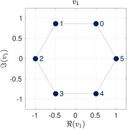
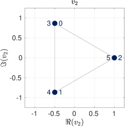
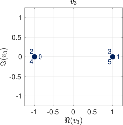
   (a) $N=6$

   

   

   

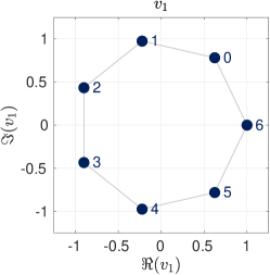
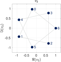
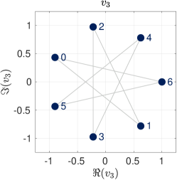
   (b) $N=7$

   Figure 5: Visualization of the complex-valued eigenvectors $v_{j}\in\mathbb{C}^{N}$, $j\neq 0$, of a circulant matrix in the complex plane for (a) $N=6$ and (b) $N=7$. Here, the number $i$ next to the blue dots correspond to $i$-th entry of $v_{j}\in\mathbb{C}$. The connections in gray between the points illustrate the (cyclically) ascending index $i=0,1,\dots,N-1$. In particular, it does not indicate any dynamical influences according to an underlying interaction graph, i.e., the generating vector $w\in\mathbb{R}^{N}$. Note that, by definition all points are on the unit circle and thus form a regular $N$-polygon (see (15)). For increasing $j$, if $N=2k$ is even, the $N$-polygon ’degenerates’ since some entries are the same, while for $N=2k+1$ only the ordering changes.
   Later on, we assign to every entry of $v_{j}\in\mathbb{C}$ its corresponding robot such that the dots also represent the position $x_{i}=\Re((v_{j})_{i}))$ and $y_{i}=\Im((v_{j})_{i})$ of the $i$-th robot in the Eulidean plane (by changing the axis labels accordingly). Hence, the generating configuration of the stable invariant subspace $V_{j}\subseteq\mathbb{R}^{2N}$ in the Euclidean plane is also visualized (cf. (23)).

With Proposition 4.1 at hand the fundamental solutions (13) of (7) for a circulant weight matrix reduce to

$$\widetilde{Z}_{j}^{x}(t)=e^{(\lambda_{j}-1)t}\begin{pmatrix}v_{j}\\ 0\end{pmatrix}\text{ and }\widetilde{Z}_{j}^{y}(t)=e^{(\lambda_{j}-1)t}\begin{pmatrix}0\\ v_{j}\end{pmatrix}\text{ for }j=0,\dotsc,N-1$$

as there are no generalized eigenvectors. However, for $j\neq 0$, the eigenvector $v_{j}$ and its corresponding eigenvalue $\lambda_{j}$ is, in general, complex-valued, which gives little to none possibility for interpretation in terms of configurations of $N\in\mathbb{N}$ robots moving in the two-dimensional Euclidean plane.

To this end, we proceed as follows: Let $N=2k$ be even or $N=2k+1$ be odd. First, for any $j=1,\dotsc,k$, we consider the pair $v_{j}\in\mathbb{C}^{N}$ and its complex conjugate $\overline{v_{j}}=v_{N-j}\in\mathbb{C}^{N}$ and define the subspace $\widetilde{V}_{j}\subseteq\mathbb{R}^{N}$ spanned by the real- and imaginary parts of $v_{j}$ and $v_{N-j}$, which is

$$\widetilde{V}_{j}=\operatorname{span}\left(\Re(v_{j}),\Im(v_{j})\right)\subseteq\mathbb{R}^{N}.$$ (18)

For $N=2k$ even, $\widetilde{V}_{k}$ simply becomes $\widetilde{V}_{k}=\operatorname{span}\left(v_{k}\right)\subseteq\mathbb{R}^{N}$, since $v_{k}$ has in fact real-valued entries (cf. Remark 4.2 (b)).

Note that by construction we have

$$W\begin{pmatrix}\Re(v_{j}),\Im(v_{j})\end{pmatrix}=\begin{pmatrix}\Re(v_{j}),\Im(v_{j})\end{pmatrix}\begin{pmatrix}\Re(\lambda_{j})&\Im(\lambda_{j})\\ -\Im(\lambda_{j})&\Re(\lambda_{j})\end{pmatrix}.$$ (19)

since the pair of eigenvalues $\lambda_{j}\in\mathbb{C}$ and $\overline{\lambda_{j}}=\lambda_{N-j}$ act as a matrix of the form

$$\Lambda_{j}=\begin{pmatrix}\Re(\lambda_{j})&\Im(\lambda_{j})\\ -\Im(\lambda_{j})&\Re(\lambda_{j})\end{pmatrix}\in\mathbb{R}^{2\times 2}.$$

in the subspace $\widetilde{V}_{j}\subseteq\mathbb{R}^{N}$. For $N=2k$ even, (19) reduces to the eigenvalue equation $Wv_{k}=\Lambda_{k}v_{k}$ for $\Lambda_{k}=\lambda_{k}\in\mathbb{R}$. Moreover, we set $\widetilde{V}_{0}=\operatorname{span}\left(v_{0}\right)$ and $\Lambda_{0}=\lambda_{0}=1$.

Using this new decomposition $\mathbb{R}^{N}=\bigoplus_{j=0}^{k}\widetilde{V}_{j}$ the weight matrix $W\in\mathbb{R}^{N\times N}$ becomes a block-diagonal matrix of the form

$$\widetilde{V}^{-1}W\widetilde{V}=\begin{pmatrix}\Lambda_{0}&&&\\ &\Lambda_{1}&&\\ &&\ddots&\\ &&&\Lambda_{k}\end{pmatrix}\in\mathbb{R}^{N\times N}\text{ with }\widetilde{V}=\left(\widetilde{V}_{0}\dotsb\widetilde{V}_{k}\right)\in\mathbb{R}^{N\times N},$$ (20)

where by abusing the notation $\widetilde{V}_{j}$ is also the matrix containing the basis vectors of $\widetilde{V}_{j}$ (cf. (18)) as its columns. For brevity we will use this double meaning from now on.

Now, recall that in the model (7) we observe a block-diagonal structure in $\mathbf{\widetilde{W}}\in\mathbb{R}^{2N\times 2N}$, which corresponds to the disconnected dynamical behavior of both coordinates of all robots. Hence, the subspace $\widetilde{V}_{j}\subseteq\mathbb{R}^{N}$ can be considered as either $x$- or $y$-coordinates and thus we set

$$V^{x}_{j}=\operatorname{span}\left(\begin{pmatrix}\Re(v_{j})\\ 0\end{pmatrix},\begin{pmatrix}\Im(v_{j})\\ 0\end{pmatrix}\right)\subseteq\mathbb{R}^{2N}\text{ and }V^{y}_{j}=\operatorname{span}\left(\begin{pmatrix}0\\ \Re(v_{j})\end{pmatrix},\begin{pmatrix}0\\ \Im(v_{j})\end{pmatrix}\right)\subseteq\mathbb{R}^{2N}.$$

As both $V^{x}_{j}\subseteq\mathbb{R}^{N}$ and $V^{x}_{j}\subseteq\mathbb{R}^{N}$ correspond to the same eigenvalue(s), we build their direct sum and define

$$V_{j}=V_{j}^{x}\oplus V_{j}^{y}=\operatorname{span}\left(\begin{pmatrix}\Re(v_{j})\\ 0\end{pmatrix},\begin{pmatrix}\Im(v_{j})\\ 0\end{pmatrix},\begin{pmatrix}0\\ \Re(v_{j})\end{pmatrix},\begin{pmatrix}0\\ \Im(v_{j})\end{pmatrix}\right)\subseteq\mathbb{R}^{2N},$$ (21)

which by construction is an invariant subspace of the model (7). In fact, any initial configuration in $V_{j}^{x,y}\subseteq\mathbb{R}^{N}$ stays in $V_{j}^{x,y}\subseteq\mathbb{R}^{N}$ as time proceeds since the matrix is block-diagonal by changing coordinates (see (20)).

For this decomposition $\mathbb{R}^{2N}=\bigoplus_{j=0}^{k}V_{j}$ the matrix $\mathbf{\widetilde{W}}\in\mathbb{R}^{2N\times 2N}$ in (7) becomes

$$V^{-1}\widetilde{W}V=\begin{pmatrix}\Lambda_{0}&&&\\ &\Lambda_{0}&&\\ &&\Lambda_{1}&&\\ &&&\Lambda_{1}&\\ &&&&\ddots&&\\ &&&&&\Lambda_{k}&\\ &&&&&&\Lambda_{k}\end{pmatrix}\in\mathbb{R}^{2N\times 2N}$$ (22)

with $V=\left(V_{0}\dotsb V_{k}\right)\in\mathbb{R}^{2N\times 2N}$.

For $j=0$, we recover the $2$-dimensional synchronous subspace $V_{0}=\operatorname{Syn}\subseteq\mathbb{R}^{2N}$ of all gathering points (in $\widetilde{Z}$-coordinates). If $j\neq 0$, then there is a pair of eigenvalues $\lambda_{j}\in\mathbb{C}$ and $\overline{\lambda_{j}}=\lambda_{N-j}\in\mathbb{C}$ (or simply $\lambda_{k}\in\mathbb{R}$ for $N=2k$ even) belonging to $V_{j}\subseteq\mathbb{R}^{2N}$ and we call the real part $\Re(\lambda_{j})\in\mathbb{R}$ convergence rate of $V_{j}\subseteq\mathbb{R}^{2N}$. Note that $\Re(\lambda_{j})<1$ for $j\neq 0$ as we assume the underlying protocol to be gathering. Hence, $V_{j}\subseteq\mathbb{R}^{2N}$ is a stable invariant subspace of (7). In particular, solutions starting in one of the $V_{j}\subseteq\mathbb{R}^{2N}$ remain in $V_{j}\subseteq\mathbb{R}^{2N}$ and converge with convergence rate $\Re(\lambda_{j})$ to $0$. The smaller $\Re(\lambda_{j})\in\mathbb{R}$ is, the faster the solution converges. As an arbitrary initial configuration $Z\in\mathbb{R}^{2N}$ can be written as a linear combination of the basis vectors of all $V_{j}\subseteq\mathbb{R}^{2N}$, we conclude that for $j\neq 0$ every part in $V_{j}\subseteq\mathbb{R}^{2N}$ vanishes as time proceeds and only the synchronous part in $V_{0}=\operatorname{Syn}\subseteq\mathbb{R}^{2N}$ remains (cf. Corollary 4.6). This part exactly represents the gathering point, i.e., the average of the initial position, as proven in Proposition 3.13.

Moreover, if there is a convergence rate $\Re(\lambda_{s})\in\mathbb{R}$ such that

$$\Re(\lambda_{s})<\Re(\lambda_{j})\quad\forall j\neq s,$$

we call $V_{s}\subseteq\mathbb{R}^{2N}$ strong stable invariant subspace. In this case, the convergence rate of any configuration in $V_{s}\subseteq\mathbb{R}^{2N}$ is faster that any configuration in any other $V_{j}\subseteq\mathbb{R}^{2N}$ for $0\neq j\neq s$.

For odd $N\in\mathbb{N}$, every subspace $V_{j}\subseteq\mathbb{R}^{2N}$, $j\neq 0$, is $4$-dimensional. However, if $N=2k$ is even, the subspace $V_{k}\subseteq\mathbb{R}^{2N}$ for $j=k$ is only $2$-dimensional which is due to the fact that $v_{k}\in\mathbb{R}^{N}$ has on real-valued entries.

Remark 4.3.

1. Our notion of convergence rate $\Re(\lambda_{j})$ of $V_{j}\subseteq\mathbb{R}^{2N}$ has to be distinguished from the definition of rate and order of convergence in the numerical analysis literature. There, a sequence $(z_{k})_{k\in\mathbb{N}}$ converging to $z^{*}$ is said to have order of convergence $p$, and with rate of convergence $\mu$, if

   $$\lim_{k\to\infty}\frac{\left\lVert z_{k+1}-z^{*}\right\rVert}{\left\lVert z_{k}-z^{*}\right\rVert^{p}}=\mu,$$

   for some positive constant $\mu>0$ if $p>1$, and $\mu\in(0,1)$ if $p=1$.

2. In fact, because we consider a linear system (5) all initial configurations converge exponentially fast to a gathering point for $t\to\infty$. Since in our linear model (7) the matrix is given by $-\mathbf{I}_{2N}+\mathbf{\widetilde{W}}\in\mathbb{R}^{2N\times 2N}$, the spectrum of $\mathbf{\widetilde{W}}\in\mathbb{R}^{2N\times 2N}$, respectively $W\in\mathbb{R}^{N\times N}$, is shifted by $-1$. Thus, the corresponding decay rates are given by $-1+\Re(\lambda_{j})$.

By definition of $V_{j}\subseteq\mathbb{R}^{2N}$ in (21) the spanning vectors correspond to configurations, where all robots have only non-zero components in one coordinate ($x$ or $y$). Thus, in particular for visualization purposes of the configurations contained in $V_{j}\subseteq\mathbb{R}^{2N}$ in the Euclidean plane, we propose the following basis instead

$$V_{j}=\operatorname{span}\left(\begin{pmatrix}\Re(v_{j})\\ \Im(v_{j})\end{pmatrix},\begin{pmatrix}\Im(v_{j})\\ \Re(v_{j})\end{pmatrix},\begin{pmatrix}\Re(v_{j})\\ -\Im(v_{j})\end{pmatrix},\begin{pmatrix}-\Im(v_{j})\\ \Re(v_{j})\end{pmatrix}\right)\subseteq\mathbb{R}^{2N}.$$ (23)

Here, the later three basis vectors (considered as points/robots in the Euclidean plane) are reflections of the first one. In this sense, we say $v_{j}\in\mathbb{C}^{N}$, respectively the configuration $\left(\Re(v_{j}),\Im(v_{j})\right)^{T}\in\mathbb{R}^{2N}$, generates the subspace $V_{j}\subseteq\mathbb{R}^{2N}$. In particular, the $x$-coordinate of the $i$-th robot is given by the real part of the $i$-the entry of $v_{j}\in\mathbb{C}^{N}$, while its $y$-coordinate is the corresponding imaginary part. Hence, the generating configuration $\left(\Re(v_{j}),\Im(v_{j})\right)^{T}\in\mathbb{R}^{2N}$ of the stable invariant subspaces $V_{j}\subseteq\mathbb{R}^{2N}$ can be visualized as in Figure 5 by simply changing the axis labels to $x$ and $y$. However, note that by choosing the adapted basis (23), the block structure into blocks $\Lambda_{j}$ in (22) is slightly destroyed as we will get $\dim V_{j}\times\dim V_{j}$-dimensional blocks instead.

Finally, we summarize the results found above in the following theorem and state that the $2N$-dimensional state space of a linear circulant gathering protocol can decomposed as follows.

Theorem 4.4.

For a linear circulant gathering protocol of $N\in\mathbb{R}$ robots there exist a family of stable invariant subspaces $\left(V_{j}\right)_{j=1}^{k}\subseteq\mathbb{R}^{2N}$ with convergence rates $\Re(\lambda_{j})<1$ and a $2$-dimensional synchronous subspace $\operatorname{Syn}\subseteq\mathbb{R}^{2N}$ such that

$$\mathbb{R}^{2N}=\operatorname{Syn}\oplus\left(\bigoplus_{j=1}^{k}V_{j}\right),\text{ where}$$ (24)

1. if $N=2k+1$ is odd, then every subspace $V_{j}\subseteq\mathbb{R}^{2N}$ is $4$-dimensional.

2. if $N=2k$ is even, then the subspace $V_{k}\subseteq\mathbb{R}^{2N}$ is $2$-dimensional, whereas the remaining $V_{j}\subseteq\mathbb{R}^{2N}$, $j\neq k$, are $4$-dimensional.

Moreover, each subspace $V_{j}\subseteq\mathbb{R}^{2N}$ is spanned by a generating eigenvector $v_{j}\in\mathbb{C}^{N}$ of the weight matrix $W\in\mathbb{R}^{N\times N}$ in the sense that

$$V_{j}=\operatorname{span}\left(\begin{pmatrix}\Re(v_{j})\\ \Im(v_{j})\end{pmatrix},\begin{pmatrix}\Im(v_{j})\\ \Re(v_{j})\end{pmatrix},\begin{pmatrix}\Re(v_{j})\\ -\Im(v_{j})\end{pmatrix},\begin{pmatrix}-\Im(v_{j})\\ \Re(v_{j})\end{pmatrix}\right)\subseteq\mathbb{R}^{2N}.$$

As indicated in Remark 4.2 (c) this decomposition in (24) is the same for every linear circulant gathering protocol. Only the explicit values of the convergence rates $\Re(\lambda_{j})$ depend on the protocol itself.

Example 4.5.

We apply Theorem 4.4 to the running examples in order to illustrate the dynamical hierarchy of the decomposition (24). To this end, we explicitly compute the eigenvalues $\lambda_{j}\in\mathbb{C}$, the corresponding convergence rates $\Re(\lambda_{j})\in\mathbb{R}$ and visualize the generating configurations $\left(\Re(v_{j}),\Im(v_{j})\right)^{T}\in\mathbb{R}^{2N}$.

1. For the $N$-bug problem we have $w=(0,1,0,\dotsc,0)^{T}\in\mathbb{R}^{N}$ (cf. Example 3.18 (a)) which by using the eigenvalue formula (16) gives us

   $$\lambda_{j}=\sum_{i=0}^{N-1}w_{i}\omega^{ij}=\omega^{j}=\exp\left(\frac{2\pi j\mathbf{i}}{N}\right)=\cos\left(\frac{2\pi j}{N}\right)+\mathbf{i}\sin\left(\frac{2\pi j}{N}\right)$$ (25)

   and thus $\Re(\lambda_{j})=\cos\left(\frac{2\pi j}{N}\right)$ for $j=0,1,\dotsc,N-1$. For some choices of $N\in\mathbb{N}$ we illustrate the convergence rates in Figure 6.

   

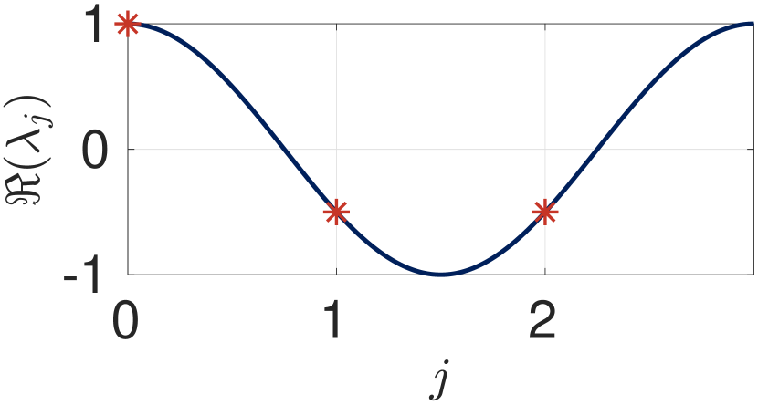
   (a) $N=3$

   

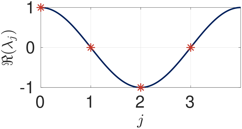
   (b) $N=4$

   

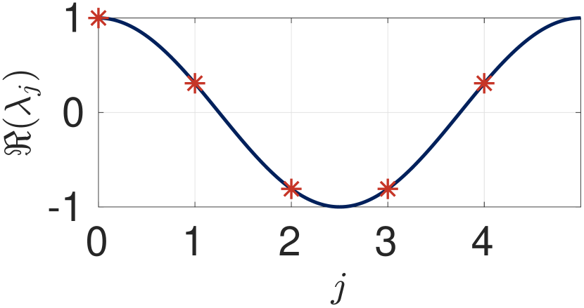
   (c) $N=5$

   

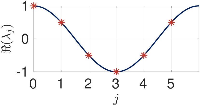
   (d) $N=6$

   

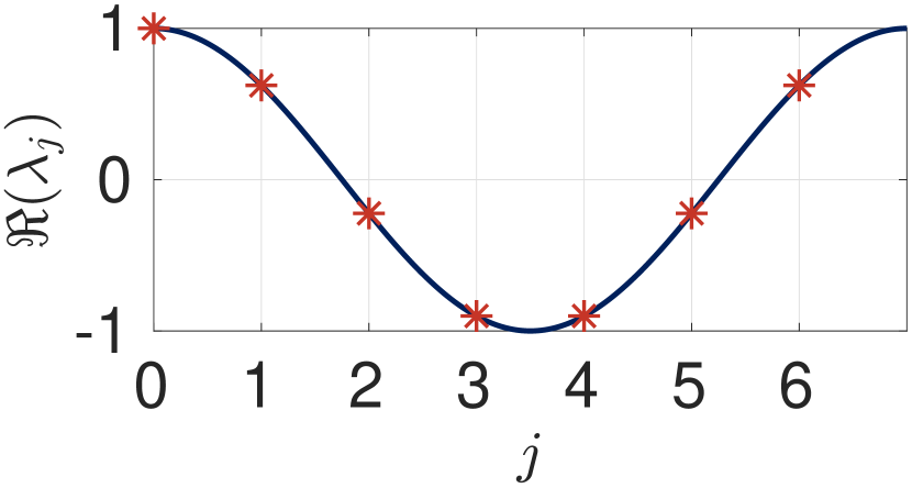
   (e) $N=7$

   

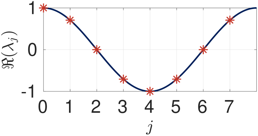
   (f) $N=8$

   Figure 6: Illustration of the convergence rates $\Re(\lambda_{j})$ of the $N$-bug problem and the Go-To-The-Middle protocol for $N\in\left\{\,3,\dotsc,8\,\right\}$ by red stars. For reference the cosine curve is also plotted in blue. As observed in Remark 4.2 (b) the convergence rates $\Re(\lambda_{j})$ are symmetrically distributed (for $j\neq 0$).

   Note that they are strictly decreasing in $j$ (up to $k$), i.e., $\Re(\lambda_{j})>\Re(\lambda_{j+1})$ for $j<k$. Hence, the stable subspaces $V_{j}\subseteq\mathbb{R}^{2N}$ are hierarchically ordered such that any configuration $Z\in V_{j}$ converges faster to a gathering point than any other configuration $\widetilde{Z}\in V_{i}$ for $i<j$. For $N=6$ and $N=6$ their generating configurations are visualized in Figure 5.

   In particular, this model has a strong stable subspace $V_{k}\subseteq\mathbb{R}^{2N}$ with corresponding convergence rate $\Re(\lambda_{k})=\cos\left(\frac{2\pi k}{N}\right)$. For $N=2k$ even, this strong stable subspace is $2$-dimensional and $\Re(\lambda_{k})=-1$. Its generating configuration is illustrated in the right panel of Figure 5(a). On the other hand, for $N=2k+1$ odd, it is $4$-dimensional with $\Re(\lambda_{k})=\cos\left(\frac{2\pi k}{2k+1}\right)$. This is due the fact that the multiplicity of the eigenvalue $\lambda_{k}$ is doubled in $X$- and $Y$-coordinates.

2. Since the Go-To-The-Middle protocol is symmetric, we have real-valued eigenvalues $\lambda_{j}\in\mathbb{R}$ (cf. Remark 4.2 (b)), i.e., they coincide with the convergence rates $\Re(\lambda_{j})$. Using the eigenvalue formula (16) with $w=(0,\frac{1}{2},0,\dotsc,\frac{1}{2})^{T}\in\mathbb{R}^{N}$ we compute

   $$\lambda_{j} =\Re(\lambda_{j})=\frac{1}{2}\Re\left(\omega^{j}\right)+\frac{1}{2}\Re\left(\omega^{(N-1)j}\right)$$

   $$=\frac{1}{2}\cos\left(\frac{2\pi j}{N}\right)+\frac{1}{2}\cos\left(\frac{2\pi j(N-1)}{N}\right)$$

   $$=\cos\left(\frac{2\pi j}{N}\right)\text{ for }j=0,\dots,N-1.$$

   Observe that the convergence rates for this protocol are the same as for the $N$-bug problem discussed in (a) whose rates are illustrated in Figure 6. In particular, we obtain the same hierarchical decomposition. Note that, from the dynamical systems perspective both models gather at the same speed. As the decomposition (24) is independent of the generating vector $w\in\mathbb{R}^{N}$, the generating configurations are also visualized in Figure 5.

3. The generating weight vector $w=(\frac{1}{N},\dotsc,\frac{1}{N})^{T}\in\mathbb{R}^{N}$ of the Go-To-The-Average protocol yields the eigenvalues

   $$\lambda_{j}=\frac{1}{N}\sum_{i=0}^{N-1}\omega^{ij}=\begin{cases}1,&\text{if }j=0,\\ 0,&\text{if }j\neq 0,\end{cases}$$

   since the average of the $N$-th roots of unity vanishes for $j\neq 0$. Again, by the symmetry of the protocol all eigenvalues $\lambda_{j}$ are indeed real and thus coincide with the convergence rates. In particular, for this protocol we have $\Re(\lambda_{j})=0$ for all $j\neq 0$ and every configuration converges with the same speed. Even though Theorem 4.4 decomposes the state space into stable subspaces $V_{j}\subseteq\mathbb{R}^{2N}$ (also shown in Figure 5), they cannot be distinguished by their convergence rates $\Re(\lambda_{j})\in\mathbb{R}$.

For the dynamics of a given arbitrary initial configuration $\widetilde{Z}\in\mathbb{R}^{2N}$ an immediate consequence of Theorem 4.4 is the following.

Corollary 4.6.

Let $\widetilde{Z}(0)=(X(0),Y(0))\in\mathbb{R}^{2N}$ be an initial configuration and the state space $\mathbb{R}^{2N}$ be decomposed as in (24). Then the solution $\widetilde{Z}(t)\in\mathbb{R}^{2N}$ of the linear gathering protocol (7) with initial condition $\widetilde{Z}(0)\in\mathbb{R}^{2N}$ can be written as

$$\widetilde{Z}(t)=\widetilde{Z}^{*}+\sum_{j=1}^{k}\alpha_{j}(t)~{}\Xi_{j}(t),\text{ where}$$ (26)

1. $\widetilde{Z}^{*}=(X^{*},Y^{*})=(x^{*},\dotsc,x^{*},y^{*},\dotsc,y^{*})$ is the final gathering point of $\widetilde{Z}\in\mathbb{R}^{2N}$. In particular, $x^{*}=\frac{1}{N}\sum_{i=0}^{N-1}X_{i}(0)$ and $y^{*}=\frac{1}{N}\sum_{i=0}^{N-1}Y_{i}(0)$.

2. $\alpha_{j}(t)=\exp((-1+\Re(\lambda_{j}))t)\in\mathbb{R}$ is the exponentially decaying coefficient corresponding to $\Xi_{j}(t)\in V_{j}$.

3. by abusing notation, $\Xi_{j}(t)=V_{j}\beta_{j}(t)$ for some coefficient vector $\beta_{j}(t)\in\mathbb{R}^{\dim V_{j}}$ with constant norm, i.e., $\left\lVert\beta_{j}(t)\right\rVert=\left\lVert\beta_{j}(0)\right\rVert$ for all $t\geq 0$.

Example 4.7.

To conclude the article, we illustrate the consequences of Corollary 4.6 for the $N$-bug problem. For $N=7$, we show in Figure 7(a) a random initial configuration $\widetilde{Z}\in\mathbb{R}^{2N}$ as well as its final gathering point $\widetilde{Z}^{*}\in\mathbb{R}^{2N}$. The corresponding exponentially decaying coefficients $\alpha_{j}(t)\in\mathbb{R}$ are plotted in Figure 7(b).

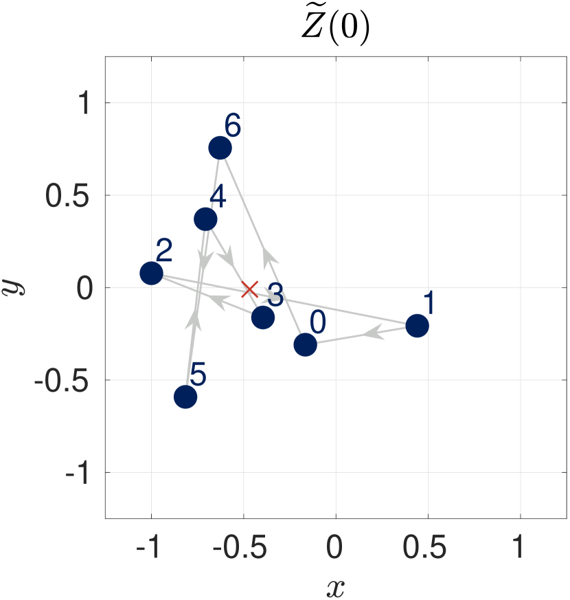
(a) Random initial configuration $\widetilde{Z}(0)\in\mathbb{R}^{2N}$ and its gathering point $\widetilde{Z}^{*}\in\mathbb{R}^{2N}$ (red cross)

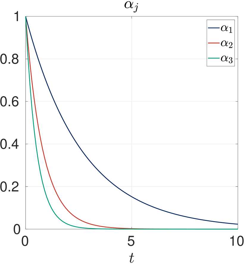
(b) Trajectory of the corresponding decaying coefficients $\alpha_{j}(t)\in\mathbb{R}$ of $\widetilde{Z}(t)\in\mathbb{R}^{2N}$

Figure 7: Visualization of a random initial configuration $\widetilde{Z}(0)\in\mathbb{R}^{2N}$ and its gathering point $Z^{*}\in\mathbb{R}^{2N}$ (red cross) in the Euclidean plane for $N=7$ in (a). Its corresponding decaying coefficients $\alpha_{j}(t)\in\mathbb{R}$ are shown in (b). Note that $\alpha_{j}(t)\in\mathbb{R}$ decreases faster for increasing $j$, which illustrates the dynamical hierarchy discussed in Example 4.5 (a).

Moreover, the initial decomposition into $\Xi_{j}(0)\in V_{j}$ is visualized in Figure 8(a), whereas the coefficients $\beta_{j}(t)\in\mathbb{R}^{\dim V_{j}}$ are shown in Figure 8(b).

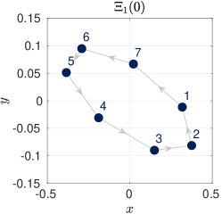
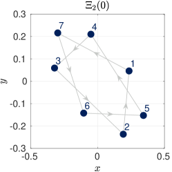
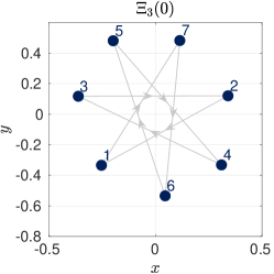
(a) Initial decomposition of $\widetilde{Z}(0)$ into $\Xi_{j}(0)\in V_{j}$

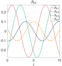
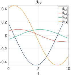
(b) Trajectory of the corresponding coefficients $\beta_{j}(t)\in\mathbb{R}^{\dim V_{j}}$ such that $\Xi_{j}(t)=V_{j}\beta_{j}(t)\in V_{j}$

Figure 8: Illustration of the decomposition (26) and its individual dynamics. Note that $\beta_{j}(t)\in\mathbb{R}^{\dim V_{j}}$ only consists of sinusoidal curves since the decaying part is in $\alpha_{j}(t)\in\mathbb{R}$. In particular, we have $\left\lVert\beta_{j}(t)\right\rVert=\left\lVert\beta_{j}(0)\right\rVert$ for all $t\geq 0$.

A related short movie of the simulation of $\widetilde{Z}(t)\in\mathbb{R}^{2N}$ and $\Xi_{j}(t)\in V_{j}$ can be found online as a supplementary file at this page.

Appendix A Technical Details of Section 3

Proof of Proposition 3.4.

(i) $\implies$ (ii): Let us first assume that $Z^{*}\in\mathbb{R}^{2N}$ is an equilibrium point of (5). In particular, $f(Z^{*})=z^{*}$. In transformed coordinates, the equilibrium point is given by $\widetilde{Z}^{*}=(X^{*},Y^{*})=(x^{*},\dotsc,x^{*},y^{*},\dotsc,y^{*})\in\mathbb{R}^{2N}$ and the right hand side of (7) vanishes in $\widetilde{Z}^{*}\in\mathbb{R}^{2N}$. We obtain,

$$\widetilde{\mathbf{W}}\widetilde{Z}^{*}=\mathbf{I}_{2N}\widetilde{Z}^{*},$$

which is equivalent to

$$WX^{*}=X^{*}\quad\text{and}\quad WY^{*}=Y^{*}$$

Since $X^{*}=x^{*}\cdot(1,\dotsc,1)^{T}\in\mathbb{R}^{N}$, this completes the proof of the first direction.

(ii) $\implies$ (iii): Let $(1,\dotsc,1)^{T}\in\mathbb{R}^{N}$ be an eigenvector of $W\in\mathbb{R}^{N\times N}$ to the eigenvalue $1$. Then

$$\sum_{j=0}^{N-1}w_{i,j} =(W(1,\dotsc,1)^{T})_{i}$$

$$=((1,\dotsc,1)^{T})_{i}$$

$$=1$$

for all $i\in\left\{\,0,\dotsc,N-1\,\right\}$, which proves (iii).

(iii) $\implies$ (i): Assume that all rows of the weight matrix $W\in\mathbb{R}^{N\times N}$ sum to $1$ and let $Z^{*}\in\mathbb{R}^{2N}$ be an arbitrary gathering point, i.e., $\widetilde{Z}^{*}=(X^{*},Y^{*})=(x^{*},\dotsc,x^{*},y^{*},\dotsc,y^{*})\in\mathbb{R}^{2N}$ in transformed coordinates. Then

$$(WX^{*})_{i}=\sum_{j=0}^{N-1}w_{i,j}\cdot x^{*}=x^{*}$$

for all $i\in\left\{\,0,\dotsc,N-1\,\right\}$ and by the same argument also $(W^{*}Y^{*})_{i}=y^{*}$. In particular, we obtain

$$\widetilde{\mathbf{W}}\widetilde{Z}^{*}=(x^{*},\dotsc,x^{*},y^{*},\dotsc,y^{*})^{T}=\mathbf{I}_{2N}\widetilde{Z}^{*}.$$

This implies that $\widetilde{Z}^{*}\in\mathbb{R}^{2N}$ is a zero of the right hand side of (7) and in turn that $Z^{*}\in\mathbb{R}^{2N}$ is an equilibrium of (5). ∎

Proof of Proposition 3.7.

Using Proposition 3.4 it suffices to prove that no point $Z\notin\operatorname{Syn}$ is an equilibrium point of (5) if and only if the geometric multiplicity of the eigenvalue $1$ is $1$. This can be seen readily from the transformed system (7). In fact, any equilibrium satisfies

$$\left(-\mathbf{I}_{2N}+\widetilde{\mathbf{W}}\right)\widetilde{Z}=0\iff\widetilde{\mathbf{W}}\widetilde{Z}=\widetilde{Z}\iff\begin{cases}WX&=X\\ WY&=Y\end{cases}$$

in transformed coordinates $\widetilde{Z}=(X,Y)\in\mathbb{R}^{2N}$. In particular, $\widetilde{Z}\in\mathbb{R}^{2N}$ is an equilibrium outside of $\operatorname{Syn}\subseteq\mathbb{R}^{2N}$ if and only if $X\in\mathbb{R}^{N}$ or $Y\in\mathbb{R}^{N}$ is an eigenvector of $W\in\mathbb{R}^{N\times N}$ to the eigenvalue $1$ that is linearly independent of $(1,\dotsc,1)^{T}\in\mathbb{R}^{N}$. Under the given assumptions, this exists if and only if the geometric multiplicity of the eigenvalue $1$ is greater than $1$. ∎

Proof of Proposition 3.8.

(i) $\implies$ (ii): Assume that any solution of (5) converges to an equilibrium point $\overline{Z}\in\mathbb{R}^{2N}$. We first consider the case that $W\in\mathbb{R}^{N\times N}$ has an eigenvalue $\lambda\in\mathbb{C}$ with $\Re(\lambda)>1$. As a simplification, we begin with $\lambda\in\mathbb{R}$. Then $\lambda>1$ and there is a corresponding real eigenvector $\xi\in\mathbb{R}^{N}$. Note that $\widetilde{Z}(t)=\exp{((\lambda-1)t)}(\xi,0)$ is the corresponding fundamental solution for $j=1$ in (13) of the transformed system (7). In fact, one readily computes $\dot{\widetilde{Z}}(t)=(\lambda-1)\widetilde{Z}(t)$ and

$$\left(-\mathbf{I}_{2N}+\mathbf{\widetilde{W}}\right)\widetilde{Z}(t) =\exp{((\lambda-1)t)}\left(-\mathbf{I}_{2N}+\mathbf{\widetilde{W}}\right)(\xi,0)$$

$$=\exp{((\lambda-1)t)}(-1+\lambda)(\xi,0)$$

$$=(\lambda-1)\widetilde{Z}(t).$$

Since $\lambda-1>0$, we have $\|\widetilde{Z}(t)\|\to\infty$ for $t\to\infty$, which contradicts the assumption. If the eigenvalue $\lambda$ is complex the argument remains the same, however the computations become slightly more complicated. In fact, replacing $\widetilde{Z}(t)$ with $\Re(\exp{((\lambda-1)t)}(\xi,0))$ yields the same result.

Next, consider an eigenvalue $\lambda\neq 1$ with $\Re(\lambda)=1$. That is, the eigenvalue is of the form $\lambda=1+\mathbf{i}\omega$ for some $\omega\in\mathbb{R}$. Again omitting the details, $\widetilde{Z}(t)=\Re(\exp{((\lambda-1)t)}(\xi,0))=\cos{(\omega t)}\Re(\xi,0))$ for a complex valued eigenvector $\xi\in\mathbb{C}^{N}$ is a fundamental solution of the system (7) that does not converge to any equilibrium. In fact, it is a periodic solution.

Finally, consider the case that $\lambda=1$ is an eigenvalue of $W\in\mathbb{R}^{N\times m}$ whose geometric multiplicity is less than its algebraic multiplicity. Then there exist two linearly independent vectors $\xi,\zeta\in\mathbb{R}^{N}$ such that $\xi$ is an eigenvector and $\zeta$ a corresponding generalized eigenvector, i.e., $(W-\mathbf{I}_{N})\zeta=\xi$. Then, $\widetilde{Z}(t)=(\zeta,0)+t(\xi,0)$ is a fundamental solution of (7). Once again, this solution does not converge to an equilibrium point, as $\|(\zeta,0)+t(\xi,0)\|\to\infty$ for $t\to\infty$.

(ii) $\implies$ (i): Assume that all eigenvalues $\lambda\in\mathbb{C}$ of $W\in\mathbb{R}^{N\times N}$ satisfy $\Re(\lambda)<1$ or $\lambda=1$ and that if $\lambda=1$ is an eigenvalue then its algebraic and geometric multiplicities agree. Note that for all fundamental solutions in (13) in the limit $t\to\infty$ all terms are dominated by the exponential as long as $\Re(\lambda_{i}-1)\neq 0$.

Under our assumptions, the only situation in which $\Re(\lambda_{i}-1)=0$ is given by the eigenvalue $\lambda_{1}=\dotsb=\lambda_{\ell}=1$, where $\ell$ is the algebraic and geometric multiplicity. For these eigenvalues, the two fundamental solutions in (13) are precisely of the form $Z_{i}^{x}(t)=(\xi_{i},0)$ and $Z_{i}^{y}(t)=(0,\xi_{i})$, where $\xi_{i}\in\mathbb{R}^{N}$ are the corresponding eigenvectors of $W\in\mathbb{R}^{N\times N}$ for $i=1,\dotsc,\ell$ – note that no generalised eigenvectors exist. For all other eigenvalues $\lambda_{\ell+1},\dotsc,\lambda_{k}$ we have $\Re(\lambda_{i}-1)<0$. As a result, any linear combination of the fundamental solutions converges to a linear combination of $(\xi_{1},0),\dotsc,(\xi_{k},0),(0,\xi_{1}),\dotsc,(0,\xi_{k})$. As any linear combination of eigenvectors to the eigenvalue $1$ constitutes another eigenvector, this linear combination is a zero of the right hand side of (7) and therefore an equilibrium point. ∎

Proof of Proposition 3.10.

For any two vertices $i,j\in\left\{\,0,\dotsc,N-1\,\right\}$ of the interaction graph, define $i\sim j$ if and only if there is an undirected path from $j$ to $i$ (if and only if there is an undirected path from $i$ to $j$). It can readily be seen that this constitutes an equivalence relation on $\left\{\,0,\dotsc,N-1\,\right\}$. Thus, it generates a partition $P_{1},\dotsc,P_{k}\subset V$ such that $P_{r}\neq\emptyset$, $P_{r}\cap P_{s}=\emptyset$ if $r\neq s$, and $P_{1}\cup\dotsb\cup P_{k}=\left\{\,0,\dotsc,N-1\,\right\}$, where $i,j\in P_{r}$ if and only if $i\sim j$. These partitions are called the connected components of the interaction graph. By definition, the interaction graph is weakly connected if and only if all vertices are connected via undirected paths, i.e., if and only if $k=1$.

Assume that the interaction graph is not weakly connected. Then $k\geq 2$. Define $P=P_{1}$ and $Q=P_{2}\cup\dotsb\cup P_{k}$. By construction, there are no paths between any vertices in $P$ and $Q$. In particular, there are no edges from any vertex in $P$ to any vertex in $Q$ and vice versa, i.e., $(j,i)\in E$ implies $i,j\in P$ or $i,j\in Q$. Since the interaction structure is reflected in the weight matrix $W=(w_{i,j})_{i,j=0}^{N-1}$, this in particular implies that $w_{i,j}=0$ whenever $i\in P$ and $j\in Q$ or $i\in Q$ and $j\in P$.

Then, we define $Z^{*}=(z_{1}^{*},\dotsc,z_{N}^{*})^{T}\in\mathbb{R}^{2N}$ as

$$z_{i}^{*}=\begin{cases}(1,1)^{T}&\text{if }i\in P,\\ 0&\text{if }i\in Q.\end{cases}$$

Considering this point as an initial configuration, we determine the robots’ behavior by applying the right hand side of (5) to it. For $i\in P$ we obtain

$$\dot{z}_{i}^{*} =-z_{i}^{*}+\sum_{j=0}^{N-1}w_{i,j}z_{j}^{*}$$

$$=-z_{i}^{*}+\sum_{j\in P}w_{i,j}z_{j}^{*}$$

$$=\left(-1+\sum_{j\in P}w_{i,j}\right)(1,1)^{T}$$

$$=\left(-1+\sum_{j=0}^{N-1}w_{i,j}\right)(1,1)^{T}.$$

As the protocol is assumed to be gathering, we have $\sum_{j=0}^{N-1}w_{i,j}=1$ for all $i\in\left\{\,0,\dotsc,N-1\,\right\}$ by Proposition 3.4 and we obtain $\dot{z}_{i}^{*}=0$. Similarly, for $i\in Q$ we compute

$$\dot{z}_{i}^{*} =-z_{i}^{*}+\sum_{j\in Q}w_{i,j}z_{j}^{*}$$

$$=\left(-1+\sum_{j\in Q}w_{i,j}\right)0$$

$$=0.$$

Combining these two computations, we see that $Z^{*}\in\mathbb{R}^{2N}$ is an equilibrium point of (5). However, as $Z^{*}\notin\operatorname{Syn}$, the protocol cannot be gathering due to Proposition 3.7. ∎

Proof of Proposition 3.12.

Recall that the weight matrix $W\in\mathbb{R}^{N\times N}$ is irreducible, if the underlying interaction graph is strongly connected. As furthermore all entries of $W\in\mathbb{R}^{N\times N}$ are non-negative, we may apply the Perron-Frobenius theorem for non-negative matrices (e.g. [Gan09, Theorem 2]). It tells us that the spectral radius $\rho(W)=\max\{|\lambda_{1}|,\dotsc,|\lambda_{k}|\}$, where $\lambda_{1},\dotsc,\lambda_{k}$ are the eigenvalues of $W\in\mathbb{R}^{N\times N}$, is itself an eigenvalue $\lambda=\rho(W)$ of $W\in\mathbb{R}^{N\times N}$. It is called the Perron-Frobenius eigenvalue, which is real by definition and all eigenvalues satisfy $|\lambda_{i}|\leq\lambda$. Furthermore, according to the Perron-Frobenius theorem, the Perron-Frobenius eigenvalue is simple. In particular, this implies $\Re(\mu)<\lambda$ for all eigenvalues $\mu\neq\lambda$, since $\lambda$ is real. Finally, note that for irreducible, non-negative matrices the Perron-Frobenius eigenvalue is also bounded by the minimal and maximal row sums of $W\in\mathbb{R}^{N\times N}$ [Gan09, Remark 2], i.e.,

$$\min_{i}\sum_{j=0}^{N-1}w_{i,j}\leq\lambda\leq\max_{i}\sum_{j=0}^{N-1}w_{i,j}.$$

By assumption, all row sums satisfy $\sum_{j=0}^{N-1}w_{i,j}=1$ so that we have $\lambda=1$. To summarize, $W\in\mathbb{R}^{N\times N}$ has a simple eigenvalue $\lambda=1$ and all other eigenvalues $\mu$ satisfy $\Re(\mu)<1$. Furthermore, due to Proposition 3.4, the eigenvector to the eigenvalue $\lambda=1$ is $(1,\dotsc,1)^{T}\in\mathbb{R}^{N}$. Hence, by Theorem 3.9, the protocol is gathering. ∎

Proof of Proposition 3.13.

First, note that $W\in\mathbb{R}^{N\times N}$ has a simple eigenvalue $1$ with corresponding eigenvector $(1,\dotsc,1)^{T}\in\mathbb{R}^{N}$ with all other eigenvalues having real part less than $1$, since it models a gathering protocol. As stated before, the solution $\widetilde{Z}(t)$ with initial condition $\widetilde{Z}(0)$ of the linear system of ordinary differential equations in transformed coordinates (7) is given by a linear combination of the fundamental solutions in (13). The coefficients of this linear combination can be determined by setting $t=0$ and requiring the linear combination to be equal to $Z(0)$. Setting $t=0$ in (13), one immediately sees that all fundamental solutions are reduced to precisely one of the eigenvectors and generalized eigenvectors in (14) that has been copied into the $X$- or the $Y$-coordinates respectively. In particular, solving for the linear coefficients boils down to solving

$$X(0)=\sum_{i=1}^{k}\sum_{j=1}^{m_{i}}a_{i,j}\xi_{i,j}\quad\text{and}\quad Y(0)=\sum_{i=1}^{k}\sum_{j=1}^{m_{i}}b_{i,j}\xi_{i,j}$$ (27)

for the coefficients $a_{i,j},b_{i,j}\in\mathbb{R}$, where $\widetilde{Z}(0)=(X(0),Y(0))\in\mathbb{R}^{2N}$ is the initial condition $Z(0)$ in transformed coordinates. Since the eigenvectors and generalized eigenvectors of $W\in\mathbb{R}^{N\times N}$ constitute a basis of $\mathbb{R}^{N}$, both equations can uniquely be solved. It remains to observe that all fundamental solutions satisfy

$$\|Z_{i,j}^{x,y}(t)\|\to 0\quad\text{for}\quad t\to\infty,$$

for every eigenvalue $\lambda\neq 1$. For the simple eigenvalue $1$ the corresponding fundamental solutions are constant. Without loss of generality, we set $\lambda_{1}=1$ and $\xi_{1,1}=(1,\dotsc,1)^{T}\in\mathbb{R}^{N}$ for the corresponding eigenvector (cf. Proposition 3.4). Then we have

$$\widetilde{Z}(t)\to a_{1,1}((1,\dotsc,1)^{T},0)+b_{1,1}(0,(1,\dotsc,1)^{T})=(a_{1,1},\dotsc,a_{1,1},b_{1,1},\dotsc,b_{1,1})^{T}$$

for $t\to\infty$. In particular, the position of every robot converges to $(a_{1,1},b_{1,1})$.

It remains to show that indeed $(a_{1,1},b_{1,1})=\left(\frac{1}{N}\sum_{i=1}^{N}x_{i}(0),\frac{1}{N}\sum_{i=1}^{N}y_{i}(0)\right)$. To that end, consider (27), which describes the decomposition of $X(0)$ and $Y(0)$ into the eigenbasis of $W\in\mathbb{R}^{N\times N}$. Since the eigenvalue $\lambda_{1}=1$ is simple, the corresponding eigenspace is one-dimensional. This allows us to compute the corresponding coefficients to be

$$a_{1,1} =\frac{\langle X(0),\xi_{1,1}\rangle}{\langle\xi_{1,1},\xi_{1,1}\rangle}=\frac{1}{N}\sum_{i=1}^{N}x_{i}(0),$$

$$b_{1,1} =\frac{\langle Y(0),\xi_{1,1}\rangle}{\langle\xi_{1,1},\xi_{1,1}\rangle}=\frac{1}{N}\sum_{i=1}^{N}y_{i}(0).$$

∎

Proof of Proposition 3.14.

The real matrix $W\in\mathbb{R}^{N\times N}$ is non-defective if and only if all of its eigenvalues are real and their algebraic and geometric multiplicities coincide. If it is additionally gathering, it has a simple eigenvalue $1$ and all other eigenvalues satisfy $\lambda<1$. All fundamental solutions (13) are of the form

$$\widetilde{Z}^{x}(t)=e^{(\lambda-1)t}(\xi,0)\quad\text{or}\quad\widetilde{Z}^{y}(t)=e^{(\lambda-1)t}(0,\xi)$$

for some eigenvalue $\lambda\in\mathbb{R}$ with corresponding eigenvector $\xi\in\mathbb{R}^{n}$. As any solution $\widetilde{Z}(t)$ to (7) is a linear combination of the fundamental solutions, any coordinate entry of such a solution is a linear combination of the exponential functions $e^{(\lambda-1)t}$. More precisely, we find fixed values $\alpha_{i}^{j}\in\mathbb{R}$ for $i,j=0,\dotsc,N-1$ – given by the coordinate entries of the eigenvectors – such that

$$\widetilde{Z}_{i}(t)=\alpha_{i}^{1}e^{(\lambda_{1}-1)t}+\dotsb+\alpha_{i}^{N}e^{(\lambda_{N}-1)t},$$

where $\lambda_{0},\dotsc,\lambda_{N-1}$ are the eigenvalues counting multiplicities. We then extract the original coordinates using $z_{i}=(\widetilde{Z}_{i},\widetilde{Z}_{i+N})$ and obtain

$$=e^{(\lambda_{0}-1)t}(\alpha_{i}^{0},\alpha_{i+N}^{0})+\dotsb+e^{(\lambda_{N-1}-1)t}(\alpha_{i}^{N-1},\alpha_{i+N}^{N-1})$$

$$=e^{(\lambda_{0}-1)t}a_{i}^{0}+\dotsb+e^{(\lambda_{N-1}-1)t}a_{i}^{N-1},$$

where we have set $a_{i}^{j}=(\alpha_{i}^{j},\alpha_{i+N}^{j})$. We readily see

$$\|z_{i}(t)-z_{j}(t)\| =\|e^{(\lambda_{0}-1)t}(a_{i}^{0}-a_{j}^{0})+\dotsb+e^{(\lambda_{N-1}-1)t}(a_{i}^{N-1}-a_{j}^{N-1})\|$$

$$\leq e^{(\lambda_{0}-1)t}\|(a_{i}^{0}-a_{j}^{0})\|+\dotsb+e^{(\lambda_{N-1}-1)t}\|(a_{i}^{N-1}-a_{j}^{N-1})\|.$$

As all the $a_{i}^{j}\in\mathbb{R}^{2}$ are fixed and all eigenvalues satisfy $\lambda\leq 1$, the expression is non-increasing in $t$ which proves that no robots increase their distance. ∎

Proof of Proposition 3.19.

Throughout this proof, we use the convention that robot indices are counted $\bmod~{}N$, as outlined in Section 2.2. In particular, the equations of motion (5) become

$$\dot{z}_{i}=-z_{i}+\sum_{j=0}^{N-1}w_{j}z_{i+j}.$$ (28)

Fix $(j,i)\in E$ such that

$$\|z_{i}(0)-z_{j}(0)\|=\max_{(l,k)\in E}\|z_{k}(0)-z_{l}(0)\|.$$

That is, robots $i$ and $j$ are furthest apart initially. We drop the time-dependence in notation and compute

$$\frac{\mathrm{d}}{\mathrm{d}t}\|z_{i}-z_{j}\|^{2} =\frac{\mathrm{d}}{\mathrm{d}t}\langle z_{i}-z_{j},z_{i}-z_{j}\rangle$$

$$=2\langle z_{i}-z_{j},\dot{z}_{i}-\dot{z}_{j}\rangle$$

$$=2\left\langle z_{i}-z_{j},-z_{i}+\sum_{k=0}^{N-1}w_{k}z_{i+k}+z_{j}-\sum_{k=0}^{N-1}w_{k}z_{j+k}\right\rangle$$

$$=2\left(-\|z_{i}-z_{j}\|^{2}+\sum_{k=0}^{N-1}w_{k}\langle z_{i}-z_{j},z_{i+k}-z_{j+k}\rangle\right),$$

where we have used the linearity of the inner product and (28). Since all weights are non-negative $w_{k}\geq 0$, we may apply the Cauchy-Schwarz inequality to the remaining inner product and obtain

$$\frac{\mathrm{d}}{\mathrm{d}t}\|z_{i}-z_{j}\|^{2}\leq 2\left(-\|z_{i}-z_{j}\|^{2}+\sum_{k=0}^{N-1}w_{k}\|z_{i}-z_{j}\|\cdot\|z_{i+k}-z_{j+k}\|\right).$$ (29)

By assumption $(j,i)\in E$, which means $w_{i,j}\neq 0$, where $W=(w_{i,j})_{i,j=0}^{N-1}$. Since $W$ is a circulant matrix, we have $w_{i,j}=w_{l}$, where $l\in\left\{\,0,\dotsc,N-1\,\right\}$ is such that $j=i+l\bmod N$. Then also $i+k+l\bmod N=j+k\bmod N$ and $w_{i+k,j+k}=w_{l}\neq 0$ for any $k\in\left\{\,0,\dotsc,N-1\,\right\}$. Thus, also $(j+k,i+k)\in E$. In particular, this implies that the sum in (29) contains only terms $\|z_{i+k}-z_{j+k}\|$ for $(j+k,i+k)\in E$. By assumption, these satisfy $\|z_{i+k}-z_{j+k}\|\leq\|z_{i}-z_{j}\|$. Hence, we may further estimate

$$\frac{\mathrm{d}}{\mathrm{d}t}\|z_{i}-z_{j}\|^{2} \leq 2\left(-\|z_{i}-z_{j}\|^{2}+\sum_{k=0}^{N-1}w_{k}\|z_{i}-z_{j}\|\cdot\|z_{i}-z_{j}\|\right)$$

$$=2\|z_{i}-z_{j}\|^{2}\left(-1+\sum_{k=0}^{N-1}w_{k}\right).$$

Since the protocol is assumed to be gathering, Theorem 3.16 implies the weight matrix is consistent $\sum_{k=0}^{N-1}w_{k}=1$ and we conclude

$$\frac{\mathrm{d}}{\mathrm{d}t}\|z_{i}-z_{j}\|^{2}\leq 0.$$

Hence, the distance of the two maximally distant robots cannot increase initially. By the same argument as before, we can extend this statement to arbitrary $t>0$, since we may always use $z_{0}(t),\dotsc,z_{N-1}(t)$ as a new initial configuration.

Note that we may not rule out the situation that two robots $k,l$ with $(l,k)\in E$ that are not maximally distant increase their distance. However, assume that $\|z_{k}(t^{*})-z_{l}(t^{*})\|>\mathcal{C}$ for some $t^{*}>0$. Since $\|z_{i}(t)-z_{j}(t)\|$ is non-increasing, there must be some $0<t<t^{*}$ at which $\|z_{k}(t)-z_{l}(t)\|=\|z_{i}(t)-z_{j}(t)\|\leq\mathcal{C}$ by continuity of the solution $z(t)$. Then we may again use $z_{0}(t),\dotsc,z_{N-1}(t)$ as a new initial configuration and the argument above with the roles of $(j,i)$ and $(l,k)$ switched yields that $\|z_{k}(t)-z_{l}(t)\|$ cannot increase any further contradicting the assumption. In particular, $k$ and $l$ cannot lose sight of each other. This completes the proof. ∎

References

- [ASY95] H. Ando, I. Suzuki, and M. Yamashita. Formation and agreement problems for synchronous mobile robots with limited visibility. In Proceedings of Tenth International Symposium on Intelligent Control, pages 453–460, 1995.
- [BT84] F. Boesch and R. Tindell. Circulants and their connectivities. Journal of Graph Theory, 8(4):487–499, 1984.
- [CFH+20] J. Castenow, M. Fischer, J. Harbig, D. Jung, and F. Meyer auf der Heide. Gathering anonymous, oblivious robots on a grid. Theor. Comput. Sci., 815:289–309, 2020.
- [CHJ+23] J. Castenow, J. Harbig, D. Jung, T. Knollmann, and F. Meyer auf der Heide. Gathering a euclidean closed chain of robots in linear time and improved algorithms for chain-formation. Theoretical Computer Science, 939:261–291, 2023.
- [CP04] R. Cohen and D. Peleg. Robot convergence via center-of-gravity algorithms. In R. Královic̆ and O. Sýkora, editors, Structural Information and Communication Complexity, volume 3104 of Lecture Notes in Computer Science, pages 79–88. Springer, Berlin and Heidelberg, 2004.
- [CP05] R. Cohen and D. Peleg. Convergence properties of the gravitational algorithm in asynchronous robot systems. SIAM J. Comput., 34(6):1516–1528, 2005.
- [CP06] R. Cohen and D. Peleg. Local algorithms for autonomous robot systems. In Structural Information and Communication Complexity, 13th International Colloquium, SIROCCO 2006, Chester, UK, July 2-5, 2006, Proceedings, pages 29–43, 2006.
- [Dav79] P. J. Davis. Circulant Matrices. Wiley, New York, 1979.
- [DKKM15] B. Degener, B. Kempkes, P. Kling, and F. Meyer auf der Heide. Linear and competitive strategies for continuous robot formation problems. TOPC, 2(1):2:1–2:18, 2015.
- [DKL+11] B. Degener, B. Kempkes, T. Langner, F. Meyer auf der Heide, P. Pietrzyk, and R. Wattenhofer. A tight runtime bound for synchronous gathering of autonomous robots with limited visibility. In Proceedings of the 23rd ACM Symposium on Parallelism in Algorithms and Architectures, SPAA, pages 139–148, 2011.
- [Flo19] P. Flocchini. Gathering. In Distributed Computing by Mobile Entities, Current Research in Moving and Computing, pages 63–82. Springer, 2019.
- [FPS12] P. Flocchini, G. Prencipe, and N. Santoro. Distributed Computing by Oblivious Mobile Robots. Synthesis Lectures on Distributed Computing Theory. Morgan & Claypool Publishers, 2012.
- [FPS19] P. Flocchini, G. Prencipe, and N. Santoro, editors. Distributed Computing by Mobile Entities, Current Research in Moving and Computing, volume 11340 of Lecture Notes in Computer Science. Springer, 2019.
- [FPSV17] P. Flocchini, G. Prencipe, N. Santoro, and G. Viglietta. Distributed computing by mobile robots: uniform circle formation. Distributed Computing, 30(6):413–457, 2017.
- [Gan09] F. R. Gantmacher. The theory of matrices, volume 2. American Mathematical Soc, Providence, RI, reprinted. edition, 2009.
- [Gra05] R. M. Gray. Toeplitz and circulant matrices: A review. Foundations and Trends® in Communications and Information Theory, 2(3):155–239, 2005.
- [Ham18] H. Hamann. Swarm Robotics - A Formal Approach. Springer, 2018.
- [HJPR87] J.-M. Helary, C. Jard, N. Plouzeau, and M. Raynal. Detection of stable properties in distributed applications. In Proceedings of the sixth annual ACM Symposium on Principles of distributed computing, pages 125–136, 1987.
- [HSD13] M. W. Hirsch, S. Smale, and R. L. Devaney. Differential Equations, Dynamical Systems, and an Introduction to Chaos. Academic Press, Boston, 2013.
- [IKIW07] T. Izumi, Y. Katayama, N. Inuzuka, and K. Wada. Gathering autonomous mobile robots with dynamic compasses: An optimal result. In Distributed Computing, 21st International Symposium, DISC 2007, Lemesos, Cyprus, September 24-26, 2007, Proceedings, pages 298–312, 2007.
- [Kli10] P. Kling. Unifying the analysis of communication chain strategies. Master’s thesis, Paderborn University, 2010.
- [KMadH11] P. Kling and F. Meyer auf der Heide. Convergence of local communication chain strategies via linear transformations. In F. Meyer auf der Heide, editor, Proceedings of the 23rd ACM symposium on Parallelism in algorithms and architectures, ACM Conferences, page 159, New York, NY, 2011. ACM.
- [KMadH19] P. Kling and F. Meyer auf der Heide. Continuous protocols for swarm robotics. In P. Flocchini, G. Prencipe, and N. Santoro, editors, Distributed Computing by Mobile Entities: Current Research in Moving and Computing, pages 317–334. Springer International Publishing, Cham, 2019.
- [LC08] G. Lee and N. Y. Chong. A geometric approach to deploying robot swarms. Annals of Mathematics and Artificial Intelligence, 52(2):257–280, Apr 2008.
- [LV19] G. A. D. Luna and G. Viglietta. Robots with lights. In Distributed Computing by Mobile Entities, Current Research in Moving and Computing, pages 252–277. Springer, 2019.
- [SS94] A. Schiper and A. Sandoz. Strong stable properties in distributed systems. Distributed Computing, 8(2):93–103, Oct 1994.
- [SY06] I. Suzuki and M. Yamashita. Erratum: Distributed anonymous mobile robots: Formation of geometric patterns. SIAM J. Comput., 36(1):279–280, 2006.
- [Tee07] G. J. Tee. Eigenvectors of block circulant and alternating circulant matrices. New Zealand Journal of Mathematics, 36(8):195–211, 2007.
- [Tes12] G. Teschl. Ordinary differential equations and dynamical systems, volume v.140 of Graduate Studies in Mathematics Ser. American Mathematical Society, Providence, Rhode Island, online-ausgabe edition, 2012.
- [vD86] E. A. van Doorn. Connectivity of circulant digraphs. Journal of Graph Theory, 10(1):9–14, 1986.
- [WK69] A. Watton and D. W. Kydon. Analytical aspects of the -bug problem. American Journal of Physics, 37(2):220–221, 1969.
- [Xie10] W.-C. Xie. Differential equations for engineers. Cambridge Univ. Press, Cambridge and New York, NY, 1. publ edition, 2010.