WHO-IS: Wireless Hetnet Optimization
using Impact Selection

Abstract

We propose a method to first identify users who have the most negative impact on the overall network performance, and then offload them to an orthogonal channel. The feasibility of such an approach is verified using real-world traces, network simulations, and a lab experiment that employs multi-homed wireless stations. In our experiment, as offload target, we employ LiFi IR transceivers, and as the primary network we consider a typical Enterprise Wi-Fi setup. We found that a limited number of users can impact the overall experience of the Wi-Fi network negatively, hence motivating targeted offloading. In our simulations and experiments we saw that the proposed solution can improve the collision probability with 82% and achieve a 61 percentage point air utilization improvement compared to random offloading, respectively.

1 Introduction

With the emergence of wireless IoT devices, an increased emphasis on remote video conferencing, and an ever increasing demand from new bandwidth-hungry applications, such as AR/VR, Wi-Fi networks are struggling to keep up. New spectrum availability and more spectrum efficient protocols mitigate congestion but do not fully solve the problem, due to the trade-offs involved in operating on different spectrum bands, e.g. range, throughput trade-offs. In an office environment this trend is exacerbated with dense AP and station deployments, where limited orthogonal Wi-Fi channels force use of narrower bands and hence lower throughput capacity to avoid excessive interference. In such environments, saturation of airtime utilization, and spiking collision probabilities cause packet delays that lead to a poor user experience, especially for latency-sensitive applications.

These trends have led to renewed interest in meeting the demand with heterogeneous networks (HetNets) composed of technologies and protocols operating in non-interfering spectrum bands.

One such technology often proposed for load balancing, and capacity enhancement is Light Fidelity (LiFi). The first generation of LiFi systems operated in the visible light spectrum. However, newer generations of LiFi systems use the infrared (IR) spectrum. With the introduction of IR-based as opposed to visible light communication LiFi no longer suffers from many of the initial drawbacks that made it impractical for general use, such as light dimming degradation and poor uplink performance due to glare. Furthermore, throughput performance of commercially available hardware is starting to match that of Wi-Fi. The current downsides of LiFi include expensive hardware, limited reach (line of sight, LoS), and intrusive deployments with essentially a dedicated LiFi antenna for each receiver. LiFi APs can handle tens of clients concurrently. However, the very limited range and sensitivity to receiving orientation angle (ROA) make the 1-1 mapping of antenna to receiver the most practical setup at the present time, at least until the multi-user time-slicing standards currently in development are finalized. LiFi APs typically operate on the same spectrum band, so inter-cell interference becomes an issue if deployments are too dense.

To address some of these practical problems we utilize a setup that involves a LiFi antenna that can be steered through a pan-tilt servo mount to serve one dedicated user over LiFi among a group of users within range. Beyond cost savings, there are many benefits to directing the antenna more precisely to the receiver including achieving longer distances, allowing a much larger area to be covered while mitigating inter-cell interference, and avoiding multi-user access degradation. In our experimental setup a single antenna can easily serve a cluster of four standard-sized office cubicles while mounted in a ceiling 3-4m high whereas the LiFi hardware only allows a 68% angle reach within about 2 meters, limiting it to transmit from something like an office lamp to a device on a desk. Although the technology will undoubtedly improve both in reach and angle coverage we believe the servo steering technique could be feasible to extend the range of LiFi while still providing dedicated Line of Sight (LoS) communication, which is considered to be a security benefit of LiFi.

Our primary contribution in this work is a predictive model, based on neural networks, that:

• predicts which Wi-Fi station should be offloaded to an orthogonal channel, in our case LiFi,

• given current measurements both from the primary and offloading target network

• to optimize network KPIs, such as air-time utilization and collision probability.

We validate our work with real-world trace analysis, Wi-Fi network simulations (in NS3), and a lab experiment with commercial-grade Wi-Fi and LiFi hardware and off-the-shelf end-user devices. The remainder of the paper is organized as follows.

We discuss related work in Section 2, and motivate our approach using an analysis of public Wi-Fi traces in Section 3. In Section 4 we define our problem more formally, followed by an evaluation using simulations (Section 5) and experiments (Sections 6 and 7). Finally, we provide concluding remarks in Section 8.

2 Related Work

Predicting or selecting one or more users to offload from a given network or access point to another based on some optimality criterion has been studied for a long time under the topics of “user association” and “user handoff.” For example, [1] applied a game theoretic framework to analyze association in a network with High Speed Downlink Packet Access (HSDPA) and LTE, while  [2] formulated a stochastic game to model non-cooperative users competing for limited resources from multiple cellular base stations. A general utility-optimizing formulation for user association in a heterogeneous network was proposed in [3], while [4] applied a multiple attribute decision making method with careful selection of user attributes to reduce computational complexity. Treating user association as a combinatorial optimization problem instead, a stochastic decision framework was proposed and analyzed in [5]. A fuzzy logic approach to designing handoff between a WLAN and a cellular network to reduce call dropping probability was studied in [6, 7], while [8, 9] applied a constrained Markov Decision Process formulation instead, and  [10] proposed a user association scheme based on load-balancing using a cell-breathing scheme.

To the best of our knowledge, our work is the first approach of using an auto-trained Neural Network (NN) to predict the user that is optimal to offload (e.g. from Wi-Fi to LiFi) using a KPI impact perspective. The approach has, however, been inspired by previous contributions in the areas of Machine Learning (ML) and Wi-Fi/LiFi HetNets.

2.1 ML-driven HetNets

Interference is classical problem in HetNets, and in  [11] the authors propose an ML classification and offloading scheme to improve co-tier interference between femtocells. Support Vector Machine (SVM), Random Forest (RF), Artificial Neural Networks (ANN) and Convolutional Neural Networks (CNN) are all evaluated as alternative models for interference classification and subsequent offloading decisions. CNN and RF were the top performers. Interference is similar to our collision probability KPI; however, our solution differs in the way we formulate the offloading decision, in that we try to predict the user who impacts the current network most negatively.

A reinforcement learning solution is proposed for joint power control and user association in a millimeter wave heterogeneous network in [12]. In [13], a recommender model was proposed to map users to access points (LTE or Wi-Fi), while in [14], the authors modeled the user association problem as a restless multi-armed bandit and exploited individual user behavior characteristics to maximize long-term expected system throughput. In [15] $k$-means clustering is used to classify users to improve handover decisions across HetNets based on user context. In [16] a DNN is trained offline to make optimal cache placement decisions in a HetNet.

Our approach differs from all of the above in that we can accommodate multiple KPIs into our optimization through our problem formulation based on the negative impact score.

2.2 Wi-Fi/LiFi HetNets

From the early days of LiFi there has been work considering how to best manage a hybrid Wi-Fi and LiFi HetNet network [17, 18, 19, 20, 21]. These studies were evaluated with custom simulations, and assumed fixed LiFi beam directions. They also focused on improving user satisfaction and throughput as opposed to network KPIs as in our study. Furthermore, the models proposed were either using linear programming models or optimization heuristics based on game theory or genetic algorithms. Based on the complexity of Wi-Fi alone, we believe machine learning (ML) approaches such as neural networks (NNs) are a more promising basis for a solution and would also scale better to more users.

More recently, this idea has been revisited [22] to formulate a resource allocation optimization problem minimizing delay and meeting a minimum data rate by assigning resource shares across Wi-Fi and LiFi APs. In that work, the LiFi antennas are deployed and directed statically to cover an entire meeting room. Since they allow multiple users on the same AP, they need to account for interference both on the LiFi and the Wi-Fi bands. Furthermore, since the LiFi beams are not targeted, the best signal of an AP is not guaranteed to be where the user is located who receives the signal. We believe that ML techniques such as NNs are better suited than traditional optimization problem formulations in capturing the complexity of both Wi-Fi and LiFi networks, and we think the allocations can be more efficient with dedicated LiFi channels since the beam range is so limited. Given the current cost of a LiFi antenna it is also both a cost issue and deployment hassle to litter the ceiling with one antenna for each position a device may be located. Furthermore, most office ceilings are higher than the 2m range of current LiFi transmitters.

In [23] beam forming inspired by mmWave technology is mentioned as a future direction of LiFi, and the general problem of spectrum shortage is highlighted as a future research problem where LiFi offloading could help. We also note that, according to this overview which is based on the hardware we are using, current chipsets do not support handover between Wi-Fi and LiFi and thus mobility is a problem. However, the new converged 802.11bb specification does support handover, and once that is implemented in chipsets it becomes more interesting to study which users to offload rather than making the switch more efficient, which helps explain the focus of our work.

3 Motivation

We analyze packet capture traces from Wi-Fi deployments to:

• motivate our general approach of defining and selecting so-called negative impact users to offload to LiFi (see below),

• evaluate candidate statistics as impact predictors, and

• validate some impact prediction models.

3.1 Negative Impact Score

First, we need to define what we mean by negative impact in order to identify Wi-Fi users (STAs) that are candidates for offloading to LiFi.

The trace is divided into equally-sized time segments indexed by $t=1,2,\dots$, and we then measure $r_{t}$, the overall packet retry probability across all captured packets in each time segment $t$.

We also track all users who started sending or receiving packets (entered) or stopped sending or receiving packets (dropped out) in each time segment $t$.

Suppose a new user $u$ entered the system in time segment $t$, but all other active users in time segment $t-1$ remained active in time segment $t$ and no other users entered or departed the system in time segment $t$. (This is likely to be the case if the time segments are short in duration and the system is not very heavily loaded.) Then we say that user $u$ had a negative impact on the system if the overall packet retry probability $r_{t}$ in $t$, the first time segment with user $u$ active, is greater than the overall packet retry probability $r_{t-1}$ in the previous time segment:

$$r_{t}>r_{t-1},$$ (1)

or equivalently,

$$\Delta^{\mathrm{e}}_{u,t}\equiv r_{t}-r_{t-1}>0.$$ (2)

Note that since $r_{t-1}$ and $r_{t}$ are both aggregate system measurements, so is their difference $\Delta_{t}=r_{t}-r_{t-1}$. However, because of our assumption that the only change to the system between time intervals $t-1$ and $t$ is the entry of the user $u$, we can attribute the change in overall packet retry probability to $u$, hence we are justified in attaching the subscript $u$ to $\Delta_{t}$. The superscript $\mathrm{e}$ denotes the entry of this user $u$ into the system in time segment $t$.

Similarly, suppose that user $u^{\prime}$ was active in time segment $t^{\prime}-1$ and departed the system in time segment $t^{\prime}$, while all other active users in time segment $t^{\prime}-1$ remained active in time segment $t^{\prime}$ and no other users entered or departed the system in time segment $t^{\prime}$. Then we say that user $u^{\prime}$ had a negative impact on the system if the overall packet retry probability $r_{t^{\prime}}$ in $t^{\prime}$, the first segment without user $u^{\prime}$ active, is lower than the overall packet retry probability $r_{t^{\prime}-1}$ in the previous time segment:

$$r_{t^{\prime}}<r_{t^{\prime}-1},$$ (3)

or equivalently,

$$\Delta^{\mathrm{d}}_{u^{\prime},t^{\prime}}\equiv r_{t^{\prime}}-r_{t^{\prime}-1}<0,$$ (4)

where again the subscript $u^{\prime}$ for the aggregate system measurement $\Delta_{t^{\prime}}$ is justified because of our assumptions above, and the superscript $\mathrm{d}$ denotes the departure of user $u^{\prime}$ from the system.

Now consider a single user $u$, and suppose that in the trace, $u$ is seen to enter the system in time segments $t_{1},t_{2},\dots,t_{n}$ and depart the system in time segments $t^{\prime}_{1},t^{\prime}_{2},\dots,t^{\prime}_{m}$. As before, we assume that the duration of each time segment is short enough that in each of these time segments, $u$ is the only user to either enter or depart the system, and all other users retain their state of activity or inactivity unchanged from the immediately prior time segment. We also assume that the total time for the trace is short enough for us to assume (quasi)-stationarity, so that we may model $\Delta^{\mathrm{e}}_{u,t_{1}},\dots,\Delta^{\mathrm{e}}_{u,t_{n}}$ as independent identically distributed (i.i.d.) random variables with common expected value $\mu^{\mathrm{e}}(u)$, and similarly model $\Delta^{\mathrm{d}}_{u,t^{\prime}_{1}},\dots,\Delta^{\mathrm{d}}_{u,t^{\prime}_{m}}$ as i.i.d. random variables with common expected value $\mu^{\mathrm{d}}(u)$. Note that from (2) and (4), it follows that $\mu^{\mathrm{e}}(u)>0$ and $\mu^{\mathrm{d}}(u)<0$ respectively. The mean magnitudes $|\mu^{\mathrm{e}}(u)|=\mu^{\mathrm{e}}(u)$ and $|\mu^{\mathrm{d}}(u)|=-\mu^{\mathrm{d}}(u)$ may be seen as measures of the negative impact of user $u$ entering and departing the system respectively. We can then define the Negative Impact Score (NIS) of user $u$ as the sum of the above two negative impact measures of $u$ entering and departing the system:

$$\mathrm{NIS}(u)=|\mu^{\mathrm{e}}(u)|+|\mu^{\mathrm{d}}(u)|=\mu^{\mathrm{e}}(u)-\mu^{\mathrm{d}}(u).$$ (5)

In practice, the two expectations $\mu^{\mathrm{e}}(u)$ and $\mu^{\mathrm{d}}(u)$ are estimated by

$$\hat{\mu}^{\mathrm{e}}(u)=\frac{\Delta^{\mathrm{e}}_{u,t_{1}}+\cdots+\Delta^{\mathrm{e}}_{u,t_{n}}}{n}$$ (6)

and

$$\hat{\mu}^{\mathrm{d}}(u)=\frac{\Delta^{\mathrm{d}}_{u,t^{\prime}_{1}}+\cdots+\Delta^{\mathrm{d}}_{u,t^{\prime}_{m}}}{m}$$ (7)

respectively.

3.2 STA Measurements

Since many users may enter or drop out in the same segments, an accurate negative impact score for a single user relies on sampling over many segments where users enter and drop out many times. Our metric here can thus be seen as an approximation of measuring the impact directly on a per-user basis, which is not possible in this case due to the fact that we use public data sets without this granularity. However, in a real system deployment it may be possible to predict $\mathrm{NIS}$ from STA statistics measured more directly. To determine the feasibility of different statistics we collect the following measurements from the traces for each STA:

• rx received bytes per second.

• tx sent bytes per second.

• size packet size (bytes).

• rssi RSSI signal (dBm).

• phyrate PHY rate based on MCS obtained (Mbps).

• packets number of packets.

• iat inter-arrival time of packets (s).

• retries retry probability of packets.

3.3 Data Sets

We use a public data set captured in five different venues around Portland State Univerity, Oregon (PSU) [24], as well as our own private radio capture in an Enterprise office setting (ENT). The private capture was necessary to obtain rssi and phyrate measurements, as well as to do a longitudinal study over an extended period of time (12 hours).

3.4 Impact Outliers

Given our approach of selecting individual STAs to offload to LiFi, we want to verify whether there are a few users (more than one, but not too many) with high enough negative impact scores to make it:

1. worthwhile to offload individual users to improve the overall network performance significantly, and

2. non-trivial to make the optimum selection of the user(s) to offload to LiFi.

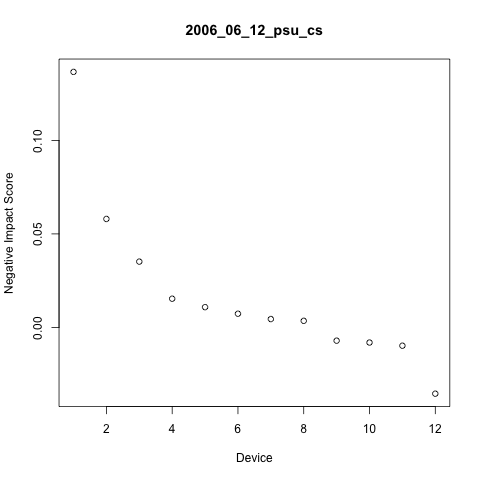
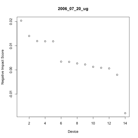
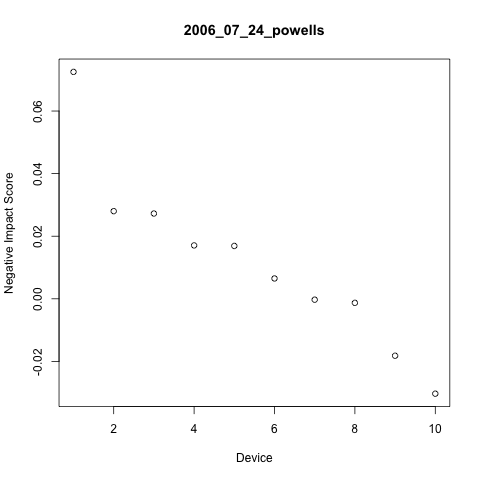
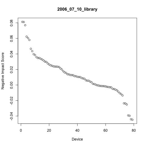
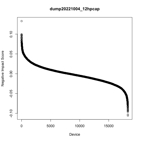
Figure 1: Ranked NIS scores

To determine whether there are outliers in terms of high negative impact we rank, and plot negative impact scores across STAs using the different data sets. Note that a higher $\mathrm{NIS}$ means that the STA has a more negative impact on the overall network, and the $x$-axis is the NIS rank of a particular user, so we are looking for outliers in the top left of the plots.

From Fig. 1 we see that all data sets revealed high NIS outliers. We should note that for some data set the top outlier was further away from the average than others as can be seen from the scale of the $y$-axis. Note that the NIS numbers are in probability units as NIS is computed from collision probabilities.

3.5 Metric Predictor Analysis

Next, we study the ability to predict NIS scores from the STA measurements listed in Sec. 3.2. We use ANOVA analyses of measurements statistics and look at F-score significance as a measure of which statistics show promise in predicting NIS for different data sets. The ANOVA analysis results can be seen in Table 1.

Table 1: Significant metrics (5% level) in ANOVA analysis for different data sets.

Data Set	Top Metric (Lowest F score)	Significant Metrics
PSU CS	rx ($1.7\times 10^{-1}$)	-
PSU UG	size ($4.3\times 10^{-4}$)	size
PSU Library	size ($1.2\times 10^{-5}$)	size, tx
PSU Powells	iat ($8.8\times 10^{-2}$)	-
ENT	size ($2\times 10^{-16}$)	size, rx, rssi, iat

3.6 Impact Class Prediction

Based on the ANOVA analysis we now take the metric deemed as the best predictor in terms of lowest F-score (see Table 1) and predict the NIS with that predictor for a random user and train with the other users. We then pick 100 different random users and compute the average prediction success rate (over these 100 predictions).

Instead of trying to predict the NIS of a user directly, we simplify the prediction problem by trying to predict only a binary value representing the tercile of this user’s NIS value: $0$ if this user’s NIS is in the top $1/3$ of all users’ NIS values, and $1$ otherwise. We also compare our model predictor with a random predictor that picks 0 with probability $1/3$ and 1 with probability $2/3$. We make this prediction in 30 rounds and compute the average and standard deviation of the success rates, shown in Table 2.

Table 2: NIS Class Prediction Mean Success Rate $\pm 1.96\sigma$.

Data Set	Linear Regression	Random
PSU CS	$.70\pm.04$	$.54\pm.05$
PSU UG	$.72\pm.03$	$.55\pm.05$
PSU Library	$.72\pm.04$	$.55\pm.04$
PSU Powells	$.67\pm.04$	$.52\pm.04$
ENT	$.74\pm.04$	$.58\pm.04$

In summary we have shown with this trace analysis that there is an opportunity to predict outlier users with a high negative impact on the overall health of the network, and that STA measurements can predict this impact.

4 Model

Each LiFi AP is enhanced with a pan-tilt unit that can orientate the AP to cover different areas. We assume a finite number $C_{l}$ of spatial configurations for LiFi AP $l$, with spatial configuration $i$ corresponding to user area (the service area for that LiFi AP configuration $i$) $u_{i,l}$, $i=1,\dots,C_{l}$. For example, in an office environment a user area could correspond to a cubicle. A LiFi AP coverage area is the union of all the user areas that can be served by the AP. We will assume that a user area can be served by at most one LiFi AP, i.e., the LiFi coverage areas do not overlap. It is worth noting that this decomposition is not an exact geometric representation of the environment.

Assuming that it is possible to collect a set of measurements for each device in the network at regular intervals on both Wi-Fi and LiFi, we denote by $\bm{w}_{n}=[w_{n,1}(t),\ldots,w_{n,K_{\mathrm{Wi}}}(t)]$ and $\bm{l}_{n}=[l_{n,1}(t),\ldots,l_{n,K_{\mathrm{Li}}}(t)]$ respectively the set of $K_{\mathrm{Wi}}$ Wi-Fi measurements and the set of $K_{\mathrm{Li}}$ LiFi measurements for device $n$ at time $t$.

For each user area $u\in\{u_{1,l},u_{2,l},\ldots,u_{C_{l},l}\}$ of LiFi AP $l$, we can aggregate the Wi-Fi and LiFi measurements of all the devices in that user area and denote the aggregated measurements as $\bm{w}_{u}^{(a)}$ and $\bm{l}_{u}^{(a)}$ respectively.

An important point to note is that we do not want “ping-ponging,” i.e., frequent transfer of an STA between Wi-Fi and LiFi, or frequent switching of the STA served by a given LiFi AP. This is similar to the ping-ponging problem of handover in a mobile cellular wireless network, and the remedy is the same, namely the use of a hysteresis factor to retain the association of an STA with a LiFi AP for a certain interval of time after the STA has been offloaded to LiFi. This hysteresis may be implemented in several ways; in the present work, we implement it by “boosting” the $\bm{l}_{u}^{(a)}$ measurements by the hysteresis factor $h_{u}^{\mathrm{LiFi}}>1$, which in general may be dependent on the user area $u$. In other words, the vector

$$\bm{E}_{l}(t)=[\bm{w}_{u_{1,l}}^{(a)},h_{u_{1,l}}^{\mathrm{LiFi}}\bm{l}_{u_{1,l}}^{(a)},\bm{w}_{u_{2,l}}^{(a)},h_{u_{2,l}}^{\mathrm{LiFi}}\bm{l}_{u_{2,l}}^{(a)},\ldots,\bm{w}_{u_{C_{l},l}}^{(a)},h_{u_{C_{l},l}}^{\mathrm{LiFi}}\bm{l}_{u_{C_{l},l}}^{(a)}]$$ (8)

contains the Wi-Fi and LiFi measurements of all the devices that can connect to LiFi AP $l$, aggregated per user area.

We model each LiFi AP as an autonomous agent that can decide which device(s) should be selected to be served by LiFi and change its orientation accordingly. Each LiFi AP makes a decision with the goal of optimizing the overall network performance $f$, which in general could be defined as a scalar function of several KPIs in the combined network. To do this, each LiFi AP learns a mapping between the current network state $\bm{E}(t)$, the possible actions, and the overall network performance. LiFi AP $l$ can use as network state the vector $\bm{E}_{l}(t)$, i.e. consider only the measurements corresponding to all the user areas in its coverage area, or it can include also additional measurements, for example the measurement vectors $\bm{E}_{j}(t)$ of nearby LiFi APs.

We can formulate the problem as a Contextual Multi-Armed Bandit (CMAB), where the network state $\bm{E}(t)$ is the context. The mapping between context, actions, and the resulting network performance may take different forms. It may be modeled as a function from the (context, action) pair to the resulting network performance. Another option is to model the mapping from context to the network performance of each action. In both cases, the mapping can be learned by a neural network.

5 Simulation

In the trace analysis we were able to show the opportunity and ability to predict the negative impact score of users to select candidates for offloading to improve the overall network performance for all users.

5.1 Layout and geometry

Since the analysis was done on static traces, we have no way of measuring the actual impact of offloading these users. Therefore, we now simulate an offloading scenario using NS3, where we model a network with only a single Wi-Fi AP containing eight users: (i) a cluster of four STAs that are candidates to be offloaded, and (ii) another cluster of four STAs that serve as background users impacting the performance.

In this simulation setup, there is no LiFi AP; instead, the effect of offloading an STA from Wi-Fi to LiFi is simulated by simply dropping that STA from the simulation, thereby allowing us to simulate only the Wi-Fi network on each NS3 run.

The four STAs that are candidates for offloading to LiFi are closer to the (Wi-Fi) AP and have average throughput 20% lower than the four other STAs that serve as background users. Although it may be counter-intuitive to have the candidate users have lower average throughput than the background users, it has the effect that any outlier (in terms of traffic) amongst the candidate users therefore has an outsize impact on the system KPIs when it drops out. At the same time, this setup allows for “headroom” for the traffic at this outlier candidate, ensuring that with high probability, even the outlier traffic does not hit (and get capped at) the maximum throughput possible in the system.

5.2 Workload trace generation

We replay workloads with a generative adversarial network (GAN)-based synthetic workload generation tool, MASS [25], trained on a public data set from Telefonica [26].

On each NS3 run, MASS is used to generate a 100-epoch long trace for each of our 8 STAs. The traces are split into multiple sections, each section of duration 10 epochs, which we call a period. The upload and download rate can vary for each STA from one period to the next. In other words, each trace may be seen as a time series of (upload, download) rate pairs for a particular STA, with as many such pairs as there are periods in the trace. Moreover, the upload and/or download rate for that STA can only change at the boundary of a period.

For each STA, each epoch of each period of the trace constitutes a MASS-generated workload with the appropriate (uplink/downlink) rate for that period, replayed for 2 ​s. Since the client iPerf processes (on the STAs) and the LiFi offload controller process (on the LiFi AP) are not synchronized, a STA may be selected for offload to LiFi at any time, and the offloading will take effect from the next epoch in the trace of that STA. The short 2-second duration of each epoch therefore ensures that the maximum delay in offloading an STA to LiFi is 2 ​s.

The maximum requested TCP download and upload rates are both set to 100 ​Mbps, and a 20 ​MHz wide 5 ​GHz 802.11ac channel is used for all STAs and the AP.

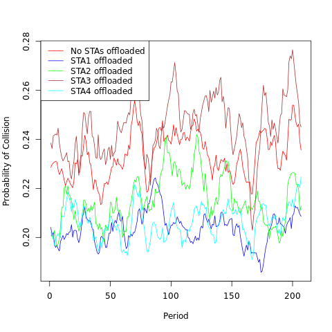
Figure 2: Simulation Collision Time Series

5.3 Statistics collected

We then run five simulations (in NS3) for each 10-epoch period in the trace, corresponding to the scenarios where no candidate STA is offloaded, and each of the four candidate STAs is offloaded respectively. For each of these five simulations in each period, we collect the pcap Wi-Fi packet trace between each STA and the AP. This allows us to capture all upload and download packets, as well as retries and other statistics such as effective send and receive rates, and packet inter-arrival times. We call the resulting statistics our measurements.

For each NS3 run, we also collect a global statistic of average retry probability across all packets sent in the system. We call this statistic the collision KPI, and it is our measure of overall network performance. The goal is to reduce this collision KPI by selecting the best STA to be offloaded (among the four candidates).

Fig. 2 shows the collision KPI for all five decisions (i.e., no STA offloaded or one of the possible four candidate STAs offloaded) during one simulation. It is clear that it is not optimal to select just one of these STAs and offload it alone throughout the entire duration of the trace.

We perform 50 NS3 runs, i.e., we repeat the steps of generating a 100-epoch (= 10-period) trace, running simulations (five per period, as described above) and collecting statistics, 50 times.

5.4 Predicting offload candidates

To evaluate different offloading predictors, we first train the prediction models with the STA measurements across all 8 STAs based on which state the system is in, i.e. no STA offloaded or, one of the four candidate STAs offloaded. During training, the prediction model output is set to the collision KPI in the next period for each of these five possible states. This setup allows us to use the model to predict the KPI in the next period, given any possible state in the current period.

5.4.1 Prediction model training and inference

The prediction models are trained with the data from the first 8 periods of the (10-period-long) traces from the 50 NS3 runs (with five simulations per period, one per state), resulting in a training set with $8\times 5\times 50=2000$ samples (#periods $\times$ #states $\times$ #simulations).

The data of the remaining 2 periods of each trace are used for testing, for a total of $2\times 50=100$ predictions (#periods $\times$ #traces). These predictions correspond to the selection of a user for offload in each of the final 2 periods of each of the 50 traces.

When predicting the best user to offload in the next period, we always assume that all four candidate STAs are present in the Wi-Fi network, i.e., the present state of the system is one where no STA has been offloaded. It should be noted that each of the 100 test predictions requires four predicted collision KPIs to be computed, one for each of the candidate STAs. The best user to offload is chosen as the STA that, when offloaded, results in the minimum collision KPI as predicted by the prediction model.

5.4.2 Prediction model evaluation

From our NS3 runs, we observed that the maximum collision probability reduction for a genie-aided (clairvoyant) predictor, which always predicts the STA that minimizes collision KPI upon being offloaded, is about $16$%. The collision improvement score, $\mathrm{cis}$, of a predictor $p$ is defined as:

$$\mathrm{cis}=\frac{P^{c}_{0}-P^{c}_{p}}{P^{c}_{0}-P^{c}_{\mathrm{cv}}}$$ (9)

where $P^{c}_{0}$ is the collision probability when no STA is offloaded, $P^{c}_{p}$ is the collision probability when the STA picked by $p$ is offloaded, and $P^{c}_{\mathrm{cv}}$ is the collision probability for the clairvoyant predictor. A clairvoyant predictor would hence have a collision improvement score of $100$%.

The prediction accuracy of predictor $p$ simply measures how many times it picked the correct STA to offload, i.e., how many times $P^{c}_{p}=P^{c}_{\mathrm{cv}}$. For a baseline, we also define the so-called random predictor, which does not attempt to predict the collision KPI upon the offloading of any of the four STAs, but instead simply directly chooses one of the four STAs at random (with the same probability $1/4$ for each STA) for offloading. Since this randomly-selected STA is expected to match the STA chosen by the clairvoyant predictor only 25% of the time, this random predictor should be expected to have a prediction accuracy of 25%.

5.4.3 Comparing predictors

We compare the performance of the following predictors, listed below in descending order of sophistication:

• : A Neural Network model;

• : A Linear Regression model;

• : A naïve model that predicts that the collision KPIs corresponding to the offloading of each of the four candidate STAs in the next period simply equal the corresponding observed collision KPIs from the simulations in the current period;

• : The baseline random predictor described above, which simply selects one of the four candidate STAs at random with the same probability of $1/4$ for offloading.

Note that even the random predictor is expected to improve the collision rate on average, as offloading any user should reduce the traffic on the channel under contention.

Table 3 shows the comparison between the different predictors. While the prediction accuracy of all models except RAND are similar, NN outperforms all the other models in terms of collision improvement score. Indeed, the prediction accuracy is not necessarily a good indicator of a predictor’s performance. For example, RAND has the lowest prediction accuracy but significantly outperforms COL in terms of reducing the collisions in the network, as measured by $\mathbf{cis}$. This happens because often, even if a predictor fails to predict the best STA to offload, the selected user is still impacting the KPI significantly. For example, if we compare the NN and LR performance, we notice that their prediction accuracy is quite close. However, NN selects STAs whose offloading improves the network performance more than that of the STAs selected by LR. In summary, we see an 82 percent improvement in collision probability when using the NN offloader compared to only 31 percent with the random model.

Table 3: Simulation Prediction Accuracy and Collision Improvement Scores ($\pm\mathit{SE}$).

Predictor	Prediction Accuracy	$\mathbf{cis}$
NN	$.51\pm.05$	$.82\pm.1$
LR	$.49\pm.05$	$.72\pm.13$
COL	$.50\pm.05$	$.31\pm.28$
RAND	$.24\pm.04$	$.47\pm.29$

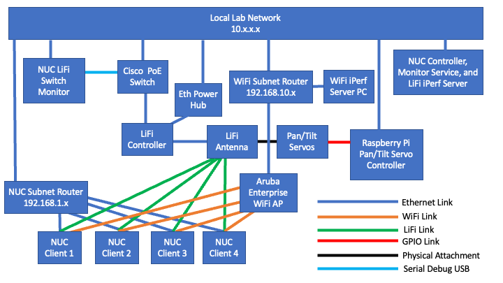
Figure 3: Physical Network Links. It should be noted that only one of the LiFi links (shown in green) is present at any given time.

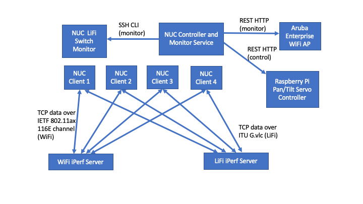
Figure 4: Communication Paths and Protocols.

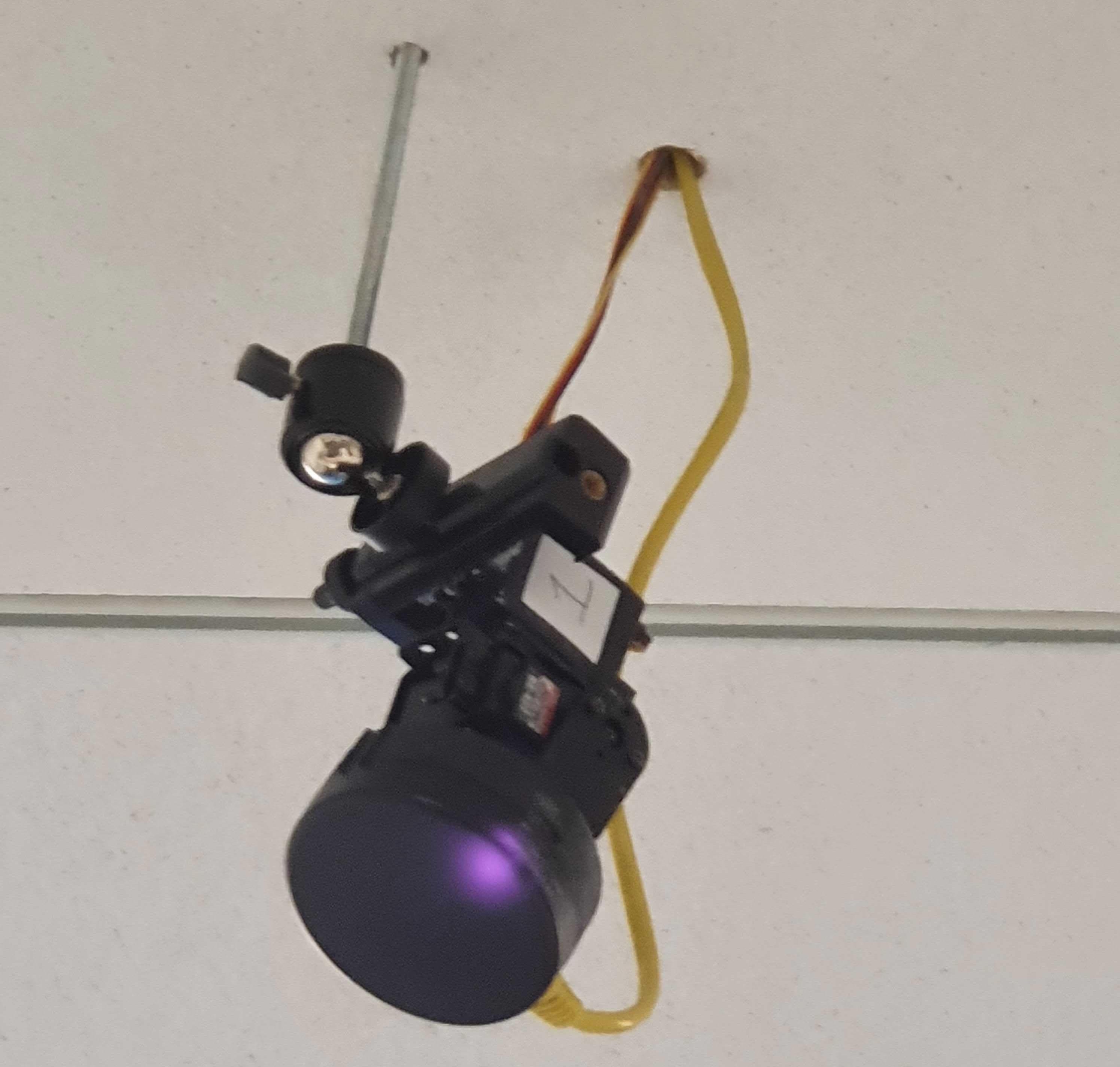
Figure 5: LiFi Antenna mounted on Pan-Tilt servos and connected to RaspberryPi in ceiling.

Figure 6: NUC with LiFi receptor dongle.

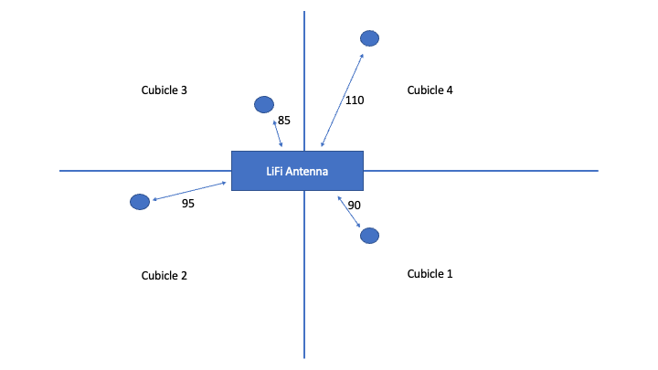
Figure 7: Experiment Setup. All distances denote shortest path from sender to receiver in inches.

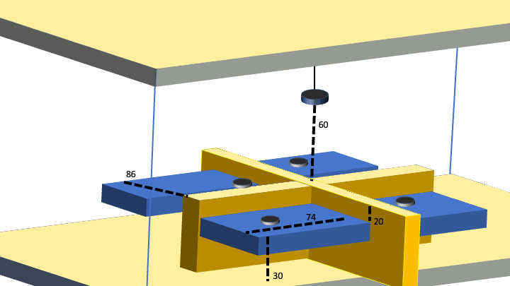
Figure 8: Experiment Setup, 3D View. All distances denote inches.

6 Experimental Setup

The purpose of our experimental system is to verify and reproduce the simulation results with real hardware radios and optical links in a lab setting that mimics an Enterprise Wi-Fi offloading use case. A key difference between simulations and experiments is also the introduction of a LiFi beam steering mechanism designed to reuse a LiFi antenna over many clients positioned in a greater area, in our case a 4-person cubicle grid. One LiFi/Wi-Fi multi-homed wireless station is placed in each cubicle.

The antenna is directed in such a way that only one wireless station or client gets dedicated LiFi connectivity at any time. All clients always have Wi-Fi to fall back on, but continuously probe and connect to LiFi if it is available. Our goal here is to improve the Wi-Fi KPI by picking the best client to offload to LiFi at any given time, based on Wi-Fi and LiFi measurements and KPI predictions.

We use LiFi hardware from Oledcomm (LiFiMax), and Wi-Fi hardware from Aruba (550 Series). To monitor the LiFi traffic we also do switch port monitoring with a Cisco switch connected to the LiFi controller, which in turn receives all LiFi traffic from the LiFi antenna.

We developed an antenna steering REST API service on a Raspberry Pi, which is connected via GPIO pins to servos controlling the angle of the LiFi antenna beams with pulse-width modulation signals. For mechanical antenna control, we use a Lynxmotion Pan and Tilt Kit with two HiTec HS-422 180 degree servo motors.

We built central offloading control and monitoring services in Python that implement the NN prediction model using Tensorlow and collect KPI and measurements from the Wi-Fi and LiFi traffic in the network. The offloading control, LiFi/Wi-Fi multi-homed clients, and the switch monitor are all deployed on Intel NUCs running Ubuntu 22.04 LTS with the 5.15 kernel.

The physical link architecture is depicted in Fig. 3 and the communication architecture in Fig. 4.

Photos of tbe LiFi AP, mounted in the ceiling, and one of the four NUC LiFi clients are shown in Fig. 5 and Fig. 6.

The LiFi client and antenna position layout is visualized in Figs. 7 and 8. The four LiFi beam positions are fixed and calibrated before the experiment and the LiFi client dongles remain stationary.

To simplify communication over different network interfaces, LiFi and Wi-Fi for experiment traffic and Wired for experiment orchestration, we created two subnets so that each interface gets an IP in a different subnet.

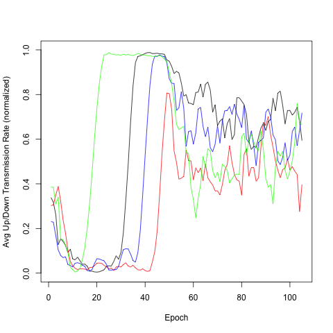
Figure 9: Workload trace used for the initial exploration stage (first quarter) and the predictions (last three quarters).

Figure 10: At the beginning of each experiment samples $\{s_{1},s_{2},\ldots,s_{T_{e}}\}$ are collected and used to train the model at time $T_{e}$. This model is used to decide the LiFi antenna orientation that will be used in the next $T_{s}$ time units, where a time unit is the time required to collect a sample. The model is updated at time $T_{e}+T_{s}$, using the most recent $T_{s}$ samples.

6.1 Traffic Replay

The four wireless stations run iPerf3 clients against two sets of iPerf3 servers, one in the LiFi subnet and one in the Wi-Fi subnet. One client-server pair is used for upload and one for download, for a total of 8 streams per iPerf server set.

It is important to ensure that the load on the CPU of the server due to iPerf does not become the bottleneck on network performance. In the LiFi case only at most two streams from a single station will be active, so the load due to iPerf is light, and the LiFi iPerf set is deployed on a NUC. On the other hand, the Wi-Fi iPerf set may in some runs serve all four STAs concurrently, so its load on the server CPU may be high. So we run the Wi-Fi iPerf set on a more powerful CPU (MacBook Air).

Traffic is generated with a specific bitrate based on trace files as in the simulation. The traces (one per station) comprise a sequence of 100 epochs, and are replayed in each experiment condition.

For each STA, each epoch of each period of the trace constitutes a MASS-generated workload with the appropriate (uplink/downlink) rate for that period, replayed for 10 ​min. The STAs use a wired connection (in order not to load the wireless network) to check for LiFi availability (with a curl to the LiFi server) every 10 ​s. Since the client processes (on the STAs) and the LiFi offload controller process (on the LiFi AP) are not synchronized, an STA may be selected for offload to LiFi at any time, and the offloading will take effect from the next epoch in the trace of that STA. Forcing the STAs to check with the LiFi offload controller every 10 ​s ensures that the maximum delay in offloading an STA to LiFi is 10 ​s.

Fig. 9 shows the total — upload and download — workload per epoch of the four STAs.

6.2 Offloading Prediction

The offloading control service monitors Wi-Fi and LiFi measurements as well as Wi-Fi KPI every 30-40s. Each experiment takes almost 17 hours and corresponds to about 1500 collected samples, where each sample consists of Wi-Fi and LiFi measurements and the corresponding KPI. We run 5 independent experiments for each of the three prediction models — NN, LR, and RAND — for a total experiment run time of about 250 ​h.

Each experiment starts with a initial exploration during which the LiFi antenna positions are selected in round-robin and $T_{e}=400$ samples (out of about 1500 total) are collected. This data is used to train the initial prediction model. This means that about the first quarter of the traces shown in Fig. 9 are used for this initial stage.

During the entire experiment, including the initial exploration, switches between LiFi positions are only allowed every $T_{s}=4$ samples, or about every 2 ​min. After the initial exploration, a prediction model is trained and used to make decisions on which station should have the LiFi antenna directed to it at any given time. Before making any new decision, the prediction model is updated with the $T_{s}=4$ most recent samples. Fig. 10 depicts this process.

7 Experiment

7.1 Defining the prediction models

As explained in Sec. 4, we formulate the problem of deciding which device should be selected for LiFi as a CMAB. In this section we evaluate different models that approximate the mapping between the (context, action) pair in the CMAB and the resulting network performance.

First, we extract air utilization ($\mathrm{air}$) as the KPI from the Aruba Wi-Fi AP on a scale from 0 to 100. Since it is more natural to consider a higher KPI better we invert these measurements as follows:

$$\mathrm{kpi}=100-\mathrm{air}$$ (10)

The goal of the proposed system is to optimize future KPI in the overall hybrid Wi-Fi/LiFi network. This is done in a two-step process: first, given the current network state $\bm{E}(t)$, a future KPI is estimated for each possible action (position), and then the actions are sorted to retrieve the top position.

We pre-process the Wi-Fi and LiFi measurements and extract features that are then used as the context $\bm{E}(t)$ of the CMAB. The most significant difference between the inputs to the models in simulation and in the experiment is the inclusion of LiFi measurements in the latter. The models trained and tested in simulation did not include LiFi measurements since no LiFi module is currently available in NS3. The other difference is that in the case of the experiment the raw Wi-Fi and LiFi measurements are processed to extract features (the impact vector explained below) to be able to train the models with a small number of samples.

7.2 Inputs to the prediction models

The input to the prediction model is the context of the CMAB, which from Sec. 4 is defined by (8)

$$\bm{E}(t)=[\bm{w}_{u_{1}}^{(a)},h^{\mathrm{LiFi}}\bm{l}_{u_{1}}^{(a)},\bm{w}_{u_{2}}^{(a)},h^{\mathrm{LiFi}}\bm{l}_{u_{2}}^{(a)},\ldots,\bm{w}_{u_{C}}^{(a)},h^{\mathrm{LiFi}}\bm{l}_{u_{C}}^{(a)}],$$

where for brevity of notation, we have dropped the LiFi AP index $l$ and assumed the same hysteresis factor $h^{\mathrm{LiFi}}$ for all $C$ user areas $u_{1},\dots,u_{C}$. In our experimental setup, $C=4$, corresponding to the four possible positions that the LiFi antenna can be pointed to. In addition to $\bm{E}(t)$, our context for the CMAB also includes the present position that the LiFi antenna is pointed to.

Since exactly one STA (among four) can be served by the LiFi antenna in each of its four positions, we further simplify $\bm{E}(t)$ by replacing the Wi-Fi and LiFi measurements in the user areas $u_{1},\dots,u_{C}$ by the corresponding quantities computed at the four STAs themselves.

The Wi-Fi measurements for the four STAs are their relative normalized traffic loads on the downlink and uplink respectively, as defined through the following Softmax operation for each direction (downlink or uplink) separately:

$$\bm{w}^{\mathrm{dir}}(t)=\mathrm{softmax}\left(\frac{N_{1}^{\mathrm{dir}}(t)-N_{1,\min}^{\mathrm{dir}}}{N_{1,\max}^{\mathrm{dir}}-N_{1,\max}^{\mathrm{dir}}},\dots,\frac{N_{4}^{\mathrm{dir}}(t)-N_{4,\min}^{\mathrm{dir}}}{N_{4,\max}^{\mathrm{dir}}-N_{4,\max}^{\mathrm{dir}}}\right),$$ (11)

where $\mathrm{dir}$ denotes the direction (uplink or downlink), and $N_{n,\min}^{\mathrm{dir}}$, $N_{n,\max}^{\mathrm{dir}}$, and $N_{n}^{\mathrm{dir}}(t)$ are respectively the minimum, maximum, and instantaneous (at time $t$) traffic load generated by STA $n$ in direction $\mathrm{dir}$, for each $n=1,\dots,4$. The softmax operation is designed to emphasize outliers, as the goal is to select the LiFi antenna position (or equivalently, the STA to be offloaded) yielding the highest performance as measured by the collision KPI.

The above vector $\bm{w}^{\mathrm{dir}}(t)$ is dense (fully populated) if no STA has been offloaded to LiFi. If an STA is offloaded from Wi-Fi to LiFi, then its corresponding entry in the vector $\bm{w}^{\mathrm{dir}}(t)$ is set to 0 and the corresponding entry in the similarly-defined vector of LiFi measurements $\bm{l}^{\mathrm{dir}}(t)$, is calculated instead and scaled by the hysteresis factor $h^{\mathrm{LiFi}}$. We have empirically determined that $h^{\mathrm{LiFi}}=3.5$ gives good results not only for the experiments reported here, but also on other workloads and in different settings.

7.3 Experimental measurements

The sampled measurements are summarized in Table 4.

Table 4: Wi-Fi and LiFi Station Measurements.

Wi-Fi	frames_in_fps
	frames_out_fps
LiFi	up_throughput
	down_throughput

The Wi-Fi measurements were collected with the Aruba REST API, and the LiFi measurements were collected using the Cisco switch CLI (using show interface summary). We note that our models normalize all measurements, so the fact that the units of different measurements are different has no impact on the predictions, and thus were chosen based on what was easiest to measure.

7.4 Evaluating the prediction models

The performance of the three predictor models is evaluated starting from the end of the initial exploration stage to the end of the traces. Let this time duration span $T$ samples, which we label $k=1,2,\dots,T$. As previously noted, each of the three models is evaluated on $E=5$ independent experiments. Let us denote by $f_{e,m}(k)$, $k=1,\dots,T$ the KPI values (airtime, in our case) observed over these samples in the experiment $e$ with prediction model $m$.

For each model $m$, we define its normalized performance over these samples as:

$$r_{e,m}(k)=\frac{f_{e,m}(k)-\min_{m}f_{e,m}(k)}{\max_{m}f_{e,m}(k)-\min_{m}f_{e,m}(k)},\quad k=1,\dots,T.$$ (12)

Then, we compute the running-average normalized performance of $m$ over these samples as:

$$[\overline{r}_{e,m}(1),\dots,\overline{r}_{e,m}(T)],$$ (13)

where $\overline{r}_{e,m}(1)=r_{e,m}(1)$ and for $k=2,\dots,T$, the $k$th element in the above is the average of the previous $k-1$ normalized performance values:

$$\overline{r}_{e,m}(k)=\frac{1}{k-1}\sum_{j=1}^{k-1}\overline{r}_{e,m}(j),\quad k=2,\dots,T.$$ (14)

Finally, we compute the running-average normalized performance of each model $m$ averaged across the $E=5$ experiments as:

$$\overline{r}_{m}(k)=(1/E)\sum_{e=1}^{E}\overline{r}_{e,m}(k)$$ (15)

Fig. 11 plots $\overline{r}_{m}(k)$ versus $k$ for $k\geq 50$, for each of the three models $m$. Table 5 summarizes the results for the different models $150$ samples after the end of the initial exploration, which is 400 samples as reported in Sec. 6.2.

Table 5: Summary of Experiment Results after 550 samples from the beginning of the experiment. CP is collision probability; LiFi is LiFi traffic multiplier compared to the optimal condition; the KPI is the average airtime across the previous 150 samples, i.e. since the end of the initial exploration stage of 400 samples, and across all experiments $e\in\{1,2,\dots,5\}$.

Model	KPI (airtime)	CP (collision probability)	LiFi
NN	$.80$	$.10$	$1.4$
LR	$.54$	$.13$	$1.1$
RAND	$.19$	$.19$	$.16$
Optimal	$1$	$.11$	$1$
Worst	$0$	$.19$	$0.41$

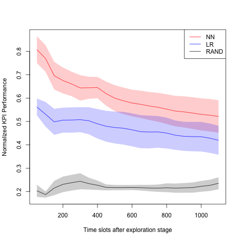
Figure 11: Plot of average normalized KPI performance $\overline{r}_{m}(\cdot)$ for each model $m$.

We note that the improvement of NN over LR is reduced the further away from training the predictions are, indicating that re-calibration or random exploration could be motivated.

In summary, we have seen that the NN model can improve the airtime utilization KPI compared to the random model with 61 percentage points (from 19% to 80%), bring the collision probability, despite not being part of the optimization, from 19% to 10%, while offloading almost a factor of 10 more traffic over the LiFi link (.16 to 1.4), in the 150 sample prediction case.

8 Discussion and Conclusion

Although our lab experiment made use of an iPerf client that is capable of detecting whether LiFi is present one cannot expect all applications to seamlessly take advantage of a new LiFi network popping up. To this end we have experimented with a number of other tools to help take advantage of both networks.

MPTCP is the most well-known technique that allows automatic subpath failover and load balancing to applications using TCP sockets. We noted that the overhead is quite large so if a subpath is very limited in throughput it is actually slower to aggregate over the paths than to use both paths. So we developed a LiFi monitor that uses a MPTCP path manager to configure the subpaths accordingly if the LiFi (or Wi-Fi) connection gets to poor.

MPHTTP is very similar to MPTCP with the difference that only the client needs to be modified to support the transmissions over multiple network interfaces. The idea here is to make use of the HTTP Range query header and schedule ranges across Wi-Fi and LiFi based on the performance of each at any given time.

MPRTP is a new protocol we developed to allow WebRTC traffic to be load balanced over LiFi and Wi-Fi and to instantaneously switch traffic from one or the other without dropping any frames in a call.

Finally, we have also experimented with network priority on MacOS that allows you to dynamically change which network interface should have highest priority. When the LiFi antenna is directed towards you we can bump the LiFi interface above the Wi-Fi interface to direct new applications to the LiFi network without interrupting existing applications.

All these use cases actively probe to see if the LiFi network is usable with either pings or various curl connection timeouts. That way they will be able to quickly take advantage of a LiFi network that comes into range. Similarly they will be able to quickly fail over to Wi-Fi when there is some temporary obstruction of LoS or the antenna is directed away from the user.

The G.vlc LiFi specification implemented in chipsets today does not support seamless handover with Wi-Fi, but the emerging 802.11bb specification defines handover support. When that specification is implemented in chipsets, approaches like ours could benefit all applications seamlessly.

We note that our MASS synthetic workload generator is based on a GAN architecture which in turn relies on a couple of DNNs, but since it its trained independently from the NN used to predict KPIs from workloads it does not taint the results.

In conclusion, we have seen in simulations and reproduced in experiments that a NN model is a promising predictor of negative impact as a basis for offloading decisions, and that the impact on network KPI can be significant even when moving just a single user.

We also note that our approach is general enough to apply to other offload use cases. For example, one could imagine using it to select the best client to steer to another band within a single technology too, such as across different Wi-Fi spectrum regions.

Appendix

A Note on LiFi Antenna Alignment

LiFi performance degrades both in terms of shortest path distance from the antenna as well as horizontal displacement from the center of the beam. Due to the latter better performance is achieved and longer distances provide connectivity if the antenna is aligned with the receiver. In the preceding experiment we pre-aligned the antenna to fixed positions of different users. A more realistic scenario is where users may be located at any number of positions in an area and we want to automatically align the antenna quickly to where the user gets the best signal.

To this end we have developed an automatic alignment algorithm that adjusts the antenna position to optimally align with the receptor. We call the algorithm pen tree alignment as it is inspired by quad tree search algorithms. The algorithm can be summarized as follows:

1. In a rectangle defining the search area pick the corners and the center as the five initial candidate positions.

2. From each candidate position measure the ping round trip times from the user device to the LiFi antenna.

3. Create a Quartic Kernel Density Estimation (Q-KDE) heat map from the candidate points, and determine the heat epicenter.

4. Divide each side of the original search area rectangle by half to produce an area 1/4 of the original area.

5. Center the new area at the epicenter and recursively run the algorithm again from the first step

6. The recursion stops as the area gets smaller and the epicenter does not change

We have experimented with this algorithm and our pan-tilt servo mechanism with promising results for areas covering meeting room attendees in a 10 person meeting room, and optical alignment could be achieved within a few seconds.

References

- [1] S. E. Elayoubi, E. Altman, M. Haddad, and Z. Altman, “A Hybrid Decision Approach for the Association Problem in Heterogeneous Networks,” in 2010 Proceedings IEEE INFOCOM, 2010, pp. 1–5.
- [2] X. Tang, P. Ren, Y. Wang, Q. Du, and L. Sun, “User association as a stochastic game for enhanced performance in heterogeneous networks,” in 2015 IEEE International Conference on Communications (ICC), 2015, pp. 3417–3422.
- [3] H. Kobayashi, E. Kameda, Y. Terashima, and N. Shinomiya, “A strategy for AP selection with mutual concessions in sustainable heterogeneous wireless networks,” in 2016 IEEE Region 10 Conference (TENCON), 2016, pp. 2788–2791.
- [4] L. Li, X. Chu, and J. Zhang, “A hierarchical MADM-based network selection scheme for system performance enhancement,” in 2014 IEEE International Conference on Communication Systems, 2014, pp. 122–126.
- [5] L. Wang, W. Chen, and J. Li, “Congestion aware dynamic user association in heterogeneous cellular network: A stochastic decision approach,” in 2014 IEEE International Conference on Communications (ICC), 2014, pp. 2636–2640.
- [6] Y. Nkansah-Gyekye and J. I. Agbinya, “Vertical Handoff between WWAN and WLAN,” in International Conference on Networking, International Conference on Systems and International Conference on Mobile Communications and Learning Technologies (ICNICONSMCL’06), 2006, pp. 132–132.
- [7] Y. Ling, B. Yi, and Q. Zhu, “An Improved Vertical Handoff Decision Algorithm for Heterogeneous Wireless Networks,” in 2008 4th International Conference on Wireless Communications, Networking and Mobile Computing, 2008, pp. 1–3.
- [8] A. Roy and A. Karandikar, “Optimal radio access technology selection policy for LTE-WiFi network,” in 2015 13th International Symposium on Modeling and Optimization in Mobile, Ad Hoc, and Wireless Networks (WiOpt), 2015, pp. 291–298.
- [9] A. Roy, V. Borkar, P. Chaporkar, and A. Karandikar, “Low Complexity Online Radio Access Technology Selection Algorithm in LTE-WiFi HetNet,” IEEE Transactions on Mobile Computing, vol. 19, no. 2, pp. 376–389, 2020.
- [10] S. Navaratnarajah, M. Dianati, and M. A. Imran, “A Novel Load-Balancing Scheme for Cellular-WLAN Heterogeneous Systems With a Cell-Breathing Technique,” IEEE Systems Journal, vol. 12, no. 3, pp. 2094–2105, 2018.
- [11] D. Anand, M. A. Togou, and G.-M. Muntean, “A Machine Learning Solution for Video Delivery to Mitigate Co-Tier Interference in 5G HetNets,” IEEE Transactions on Multimedia, 2022.
- [12] Y. Fan, Z. Zhang, and H. Li, “Message Passing Based Distributed Learning for Joint Resource Allocation in Millimeter Wave Heterogeneous Networks,” IEEE Transactions on Wireless Communications, vol. 18, no. 5, pp. 2872–2885, 2019.
- [13] B. Partov, D. J. Leith, and A. Checco, “Recommending access points to individual mobile users via automatic group learning,” in 2017 IEEE International Conference on Communications (ICC), 2017, pp. 1–6.
- [14] Y. Sun, G. Feng, S. Qin, S. Sun, and L. Zhang, “User Behavior Aware Cell Association in Heterogeneous Cellular Networks,” in 2017 IEEE Wireless Communications and Networking Conference (WCNC), 2017, pp. 1–6.
- [15] M. Xiong and J. Cao, “A clustering-based context-aware mechanism for IEEE 802.21 media independent handover,” in 2013 IEEE Wireless Communications and Networking Conference (WCNC). IEEE, 2013, pp. 1569–1574.
- [16] L. Lei, L. You, G. Dai, T. X. Vu, D. Yuan, and S. Chatzinotas, “A deep learning approach for optimizing content delivering in cache-enabled HetNet,” in 2017 international symposium on wireless communication systems (ISWCS). IEEE, 2017, pp. 449–453.
- [17] H. Haas, L. Yin, Y. Wang, and C. Chen, “What is LiFi?” Journal of lightwave technology, vol. 34, no. 6, pp. 1533–1544, 2015.
- [18] Y. Wang, X. Wu, and H. Haas, “Fuzzy logic based dynamic handover scheme for indoor Li-Fi and RF hybrid network,” in 2016 IEEE International Conference on Communications (ICC). IEEE, 2016, pp. 1–6.
- [19] X. Wu, M. Safari, and H. Haas, “Joint optimisation of load balancing and handover for hybrid LiFi and WiFi networks,” in 2017 IEEE wireless communications and networking conference (WCNC). IEEE, 2017, pp. 1–5.
- [20] Y. Wang, X. Wu, and H. Haas, “Load balancing game with shadowing effect for indoor hybrid LiFi/RF networks,” IEEE Transactions on Wireless Communications, vol. 16, no. 4, pp. 2366–2378, 2017.
- [21] M. Ayyash, H. Elgala, A. Khreishah, V. Jungnickel, T. Little, S. Shao, M. Rahaim, D. Schulz, J. Hilt, and R. Freund, “Coexistence of WiFi and LiFi toward 5G: concepts, opportunities, and challenges,” IEEE Communications Magazine, vol. 54, no. 2, pp. 64–71, 2016.
- [22] H. Vijayaraghavan and W. Kellerer, “Delay-aware Wireless Resource Allocation and User Association in LiFi-WiFi Heterogeneous Networks,” in 2021 IEEE Global Communications Conference (GLOBECOM). IEEE, 2021, pp. 01–06.
- [23] B. Béchadergue and B. Azoulay, “An Industrial View on LiFi Challenges and Future,” in 2020 12th International Symposium on Communication Systems, Networks and Digital Signal Processing (CSNDSP). IEEE, 2020, pp. 1–6.
- [24] C. Phillips and S. Singh, “Crawdad pdx/vwave (v. 2007-08-13),” 2022. [Online]. Available: https://dx.doi.org/10.15783/C7C303
- [25] T. Sandholm and S. Mukherjee, “MASS: Mobile Autonomous Station Simulation,” arXiv preprint arXiv:2111.09161, 2021.
- [26] M. Pielot, “Crawdad telefonica/mobilephoneuse,” 2022. [Online]. Available: https://dx.doi.org/10.15783/jh3s-h006