Search and study of ultracompact H II regions

Abstract

We present results from a sample of 106 high-luminosity IRAS sources observed with the Very Large Array in the B and C configurations. 96 sources were observed in the X-band and 52 in the K-band, with 42 of them observed at both wavelengths. We also used previously published observations in the C-band for 14 of them. The detection rate of sources with 3.6 cm continuum emission was $\sim 25\%$, while only 10% have emission at 1.3 cm. In order to investigate the nature of these sources, their physical parameters were calculated mainly using the 3.6 cm continuum emission, and for sources detected at two wavelengths, we used the best fit of three H II region models with different geometries. As a final result, we present a catalog of the detected sources, which includes their basic physical parameters for further analysis. The catalog contains 17 ultracompact H II regions and 3 compact H II regions.

Presentamos resultados de una muestra de 106 fuentes IRAS de alta luminosidad observadas con el interferómetro Very Large Array en las configuraciones B y C. 96 fuentes se observaron en la banda X y 52 en la banda K, con 42 de ellas observadas en ambas longitudes de onda. También usamos observaciones previamente publicadas en la banda C para 14 de ellas. La tasa de detección de fuentes con emisión de continuo a 3.6 cm fue del $\sim 25\%$, mientras que sólo un 10% tienen emisión a 1.3 cm. Para investigar la naturaleza de estas fuentes, se calcularon sus parámetros físicos usando principalmente la emisión de continuo a 3.6 cm y para fuentes detectadas en dos longitudes de onda usamos el mejor ajuste de tres modelos de regiones H II con diferentes geometrías. Como resultado final, presentamos un catálogo de las fuentes detectadas, proporcionando sus parámetros físicos básicos para su posterior análisis. El catálogo contiene 17 regiones H II ultracompactas y 3 regiones H II compactas.

ISM: H II regions ISM: General Stars: formation Radio continuum: ISM Instruments: VLA Metods: Models

0.1 Introduction

The study of high-mass star formation is crucial for understanding the physical and chemical evolution of galaxies. Because forming massive stars takes $\sim 10^{6}$ yr, the process of high mass star formation is less understood than the formation of low-mass stars (time-scales of $\sim 10^{9}$ yr). Currently, it is not completely clear how massive stars form, being monolithic collapse, protostar collision and/or coalescence, and competitive accretion the most widely accepted models (see Motte, Bontemps & Louvet, 2018, and references therein). Studying the evolution of the earliest phases of high-mass star formation is key to understanding how this process occurs. In this sense, two of the earliest phases of massive star formation are the young stellar object and the H II region(e.g Garay & Lizano, 1999). While both stages have been extensively studied, new questions continue to arise about its formation and evolution process. Further study of these evolutionary phases will undoubtedly contribute to a better understanding of massive star formation and provide evidence for or against the proposed models.

One way to contribute to solving the puzzle of high-mass star formation is to study the H II regions related to this process: the hyper-compact (HC), ultra-compact (UC), and compact H II regions. These objects are thought to be related to the evolutionary sequence as the massive star approaches the zero-age main sequence or ZAMS (e.g Beuther et al., 2007, and references therein). The Physical parameters that define HC H II , UC H II , and compact HII regions following this evolutionary sequence are shown in Table 1.

On the other hand, density gradients are highly noticeable in H II regions (e.g. De Pree, Rodriguez, & Goss, 1995; Jaffe & Martin-Pintado, 1999; Franco et al., 2000a, b, 2001; Phillips, 2007, 2008). These gradients are important and useful to describe the dynamics of a H II region. For example, density gradients with a power law of n_e $\propto$ r^β, where r is the distance from the ionization front, accurately describe expanding H II regions when $\beta\gtrsim$ 1.5 (e.g Franco, Tenorio-Tagle, and Bodenheimer, 1990; Franco et al., 2000a, b, 2001, and references therein). Thus, the presence of these gradients should be taken into consideration in models and studies of HC H II , UC H II , and compact H II regions.

In order to advance in the understanding of the earliest stages of the high-mass star formation process and to find evidence in favor of one of the models mentioned above, we perform a physical characterization of the ionized gas in a sample of 106 IRAS sources to identify H II regions in their different evolutionary stages. We calculate physical parameters at 3.6 cm in the standard way, and we apply density gradient models for sources with multiple wavelength observations. We aim to confirm if they are H II regions, and if applicable, to determine their nature and classify them as HC H II , UC H II , compact H II region, taking into consideration the presence of protostellar thermal jets.

The sample, radio continuum observations, and data reduction are described in § 0.2. Results and discussion are presented in § 0.3 and § 0.4, respectively. Finally, we give the conclusions in § 0.5 and individual sources comments are provided in Appendix 0.6.

0.2 Observations

We retrieve 3.6 and 1.3 cm data for a sample of 104 IRAS sources from the Very Large Array (VLA) archive using the B and C configurations, respectively (unpublished data from the AC295 project; P.I. Ed Churchwell). Out of the 104 sources, 94 were observed in the X band and 52 in the K band, with 42 observed at both wavelengths. We also included two sources (IRAS 18094-1823 and G45.47+0.05) observed in the X band with the VLA D configuration (AK559 project; P.I. Stan Kurtz; see de la Fuente et al. (2018, 2020a)), bringing the final sample to 106 sources. The observations of the AC295 project, at both wavelengths, were carried out in snapshot mode using a bandwidth of 50 MHz, with an integration time of 5 and 10 minutes for 3.6 and 1.3 cm, respectively, over a time span of about 4.5 months (1992 January and May) for both bands. Table 2 lists the 106 sources in the sample observed at 3.6 and 1.3 cm. Additionally, we also used 6 cm data, observed with the VLA-B and reported by Urquhart et al. (2009), for some sources detected at 3.6 and/or 1.3 cm. All sources in the sample are located in star-forming regions associated with high luminosity IRAS sources (L_FIR $\gtrsim 500$ L_⊙), and are situated more than 1 kpc away. They cover a range from $\sim 21^{h}$ to 08.5^h in right ascension (J2000), and from $\sim-41^{\circ}$ to 66^∘ in declination (J2000). These characteristics make the sources in the sample excellent candidates for identifying and studying HII regions, as well as for expanding the dataset of these objects to better understand their properties. Additional information about each source can be found in Appendix 0.6.

We performed the data editing, calibration, and further mapping of all sample sources at 3.6 and 1.3 cm wavelengths following the standard techniques using the Common Astronomy Software Applications (CASA) of the NRAO version 5.3.0-143 (McMullin et al., 2007). The flux calibrator for observations at 3.6 and 1.3 cm was 3C48, and several phase calibrators were used (see Table 3). 6 cm data were calibrated using the same procedure as was used for the 3.6 and 1.3 cm data. In order to obtain a similar angular resolution for continuum sources detected at two and three wavelengths, we convolved the data with the same beam. All observational parameters of the detected sources (position, flux density, and deconvolved angular size) were obtained with the task IMFIT of CASA.

From the subsample of 96 IRAS sources observed at 3.6 cm, we detect only 25 of them, while from the subsample of 52 sources observed at 1.3 cm, we detect only five. These five sources were also detected at 3.6 cm (see Table 4). The low detection rate may be due to the low sensitivity of the observations carried out in snapshot mode, but other reasons cannot be rule out (see subsection 0.4.1).

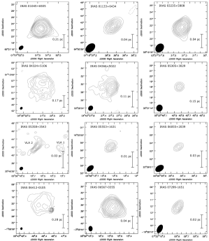
Figure 1: Continuum contour maps of the sources detected at 3.6 cm. The contours for each source are: IRAS 01045+6505: -5, 5, 10, 15, 30, 60, 90, 120, 150, 180; IRAS 01133+6434: -5, -3, 3, 5, 7, 9, 12, 15, 18, 21, 24, 27; IRAS 03235+5808: -5, -3, 3, 5, 7, 9, 12, 15, 20, 25, 30, 40, 50, 60, 70, 80; IRAS 04324+5106: -5, -3, 3, 5, 7, 9, 12, 15, 18; IRAS 04366+5022: -5, -3, 3, 5, 7, 9, 12, 15, 20, 25, 30, 35; IRAS 05305+3029: -5, -3, 3, 5, 7, 9, 12, 15, 18; IRAS 05358+3543: -5, -3, 3, 5, 7, 9, 12, 15, 18; IRAS 05553+1631: -5, -3, 3, 5, 7, 9, 12, 15, 18; IRAS 06055+2039: -5, -3, 3, 4, 5, 6, 7; IRAS 06412-0105: -5, -3, 3, 5, 7, 9, 12, 15, 20, 25, 30; IRAS 06567-0355: -5, -3, 3, 5, 7, 9, 12, 15, 20, 25, 30, 40, 50, 60, 70, 80, and IRAS 07299-1651: -5, -3, 9, 12, 15, 18, 21 times the respective rms listed in Table 5. The beam size is shown at bottom left and given in Table 5.

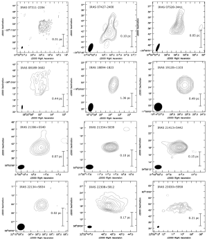
Figure 2: Continuum contour maps of the sources detected at 3.6 cm. The contours for each source are: IRAS 07311-2204: -5, -3, 3, 5, 7, 9, 12, 15, 18; IRAS 07427-2400: -5, 5, 10, 20, 40, 60, 80; IRAS 07528-3441: -5, -3, 3, 5, 7, 9, 12, 15, 20, 25, 30, 35, 40, 45; IRAS 08189-3602: -4, -3, 3, 4, 5, 7, 9, 11, 13; IRAS 18094-1823: -5, -3, 3, 5, 7, 10, 15, 20, 30, 45; IRAS 19120+1103: -5, -3, 3, 5, 7, 10, 15, 20, 30, 40, 60, 80, 100, 150, 200, 250; IRAS 21306+5540: -5, -3, 3, 5, 7, 9, 12, 15, 18, 21; IRAS 21334+5039: -5, -3, 3, 5, 7, 9, 12, 15, 20, 25, 35, 45, 55, 65, 75, 85; IRAS 21413+5442: -5, -3, 3, 5, 7, 9, 12, 15, 20, 30, 40, 60, 80, 100, 120, 140, 160, 180; IRAS 22134+5834: -5, -3, 3, 5, 7, 9, 12, 15, 18; IRAS 22308+5812: -5, -3, 3, 5, 7, 9, 11, 13, 15, 17, 19, 21, 23, and IRAS 23030+5958: -5, -3, 3, 5, 7, 9, 12, 15, 18 times the respective rms listed in Table 5. The beam size is shown at bottom left and given in Table 5.

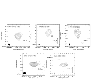
Figure 3: Contour maps of the continuum emission from sources detected at 1.3 cm The respective contour levels for each source are: IRAS 01045+6505: -5, -3, 3, 5, 10, 15, 20, 25, 30; IRAS 06412-0105: -4, -3, 3, 4, 5, 7, 9; IRAS 08189-3602: -4, -3, 3, 4, 5, 7, 9, 11; IRAS 21413+5442: -5, -3, 3, 5, 7, 9, 12, 15, 20, 30, 40, 60, 80, 100, 120, 140, 160, 180, and IRAS 23030+5958: -4, -3, 3, 4, 5, 7, 9, 11 times the respective rms reported in Table 5. The beam size is shown at bottom left and given in Table 5.

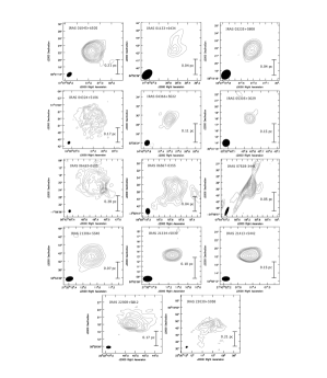
Figure 4: Continuum contour maps of the sources with 6 cm emission (these observations have been reported previously by Urquhart et al. (2009); see Section 0.2). The contours for each source are: Continuum contour maps of the sources detected at 6.0 cm. The contours for each source are: IRAS 01045+6505: 5, 10, 15, 20, 40, 60, 100, 140, 200; IRAS 01133+6434: -5, -3, 3, 5, 7, 9, 12, 15, 18; IRAS 03235+5808: -5, -3, 3, 5, 7, 9, 12, 15, 20, 30, 40, 50; IRAS 04324+5106: -5, -3, 3, 5, 7, 9, 12, 15, 18; IRAS 04366+5022: -5, -3, 3, 5, 7, 9, 12, 15, 18, 21; IRAS 05305+3029: -3, 3, 5, 7, 9, 12, 15, 18; IRAS 06412-0105: -5, -3, 3, 5, 7, 9, 12, 15, 20, 25, 30; IRAS 06567-0355: -5, -3, 3, 5, 7, 9, 12, 15, 20, 25, 30; IRAS 07528-3441: -5, -3, 3, 5, 7, 9, 12, 15, 20, 25, 30, 35, 40, 45, 50, 55; IRAS 21306+5540: -5, -3, 3, 5, 7, 9, 12, 15, 18, 21, 24; IRAS 21334+5039: -5, -3, 3, 5, 7, 9, 12, 15, 20, 30, 40, 50, 60; IRAS 21413+5442: -5, -3, 3, 5, 7, 9, 12, 15, 20, 40, 60, 100, 150, 200, 250; IRAS 22308+5812: -5, -3, 3, 5, 7, 9, 12, 15, 18, 21, 24, 27, and IRAS 23030+5958: -5, -3, 3, 5, 7, 9, 12, 15, 18 times the respective rms listed in Table 5. The beam size is shown at bottom left and given in Table 5.

Observational parameters of all detected IRAS sources at 1.3, 3.6, and 6 cm are listed in Table 5, and their respective radio contour maps are shown in Figures 1, 2, 3, and 4. Detailed results for each of the sources are provided in Appendix 0.6.

0.3 Results

0.3.1 3.6 cm Continuum Emission: Physical parameters

In order to investigate the nature of the radio continuum sources detected toward the IRAS regions, we used the 3.6 cm flux density to determine their physical parameters as if they were optically thin H II regions at this wavelength. We also assume homogeneous and isothermal gas, with an spherically symmetric distribution, composed of pure hydrogen and a canonical value for the electronic temperature of $10^{4}$ K. The electronic density (n_e), emission measure (EM), the mass of the ionized gas (M_HII), and the total rate of Lyman continuum photons of the ionizing star (N${}^{\prime}_{\rm c}$) were calculated in the standard way using equations from 1 to 4 (Schraml & Mezger, 1969; Kurtz et al., 1994):

$$\begin{split}\left(\frac{\mathrm{n_{e}}}{\mathrm{cm^{-3}}}\right)=7.8\times 10^{3}\left(\frac{\nu}{\mathrm{4.9\,GHz}}\right)^{0.05}\left(\mathrm{\frac{S_{\nu}}{mJy}}\right)^{0.5}\left(\frac{\mathrm{T_{e}}}{\mathrm{10^{4}\,K}}\right)^{0.175}\\ \times\left(\mathrm{\frac{\rm{\Theta_{s}}}{arcsec}}\right)^{-1.5}\left(\mathrm{\frac{D}{kpc}}\right)^{-0.5},\end{split}$$ (1)

$$\begin{split}\left(\frac{\mathrm{EM}}{\mathrm{pc\leavevmode\nobreak\ cm^{-6}}}\right)=4.4\times 10^{5}\left(\frac{\nu}{\mathrm{4.9\,GHz}}\right)^{0.1}\left(\mathrm{\frac{S_{\nu}}{mJy}}\right)\left(\frac{\mathrm{T_{e}}}{\mathrm{10^{4}\,K}}\right)^{0.35}\\ \times\left(\mathrm{\frac{\rm{\Theta_{s}}}{arcsec}}\right)^{-2},\end{split}$$ (2)

$$\begin{split}\left(\frac{\mathrm{M_{\rm HII}}}{\mathrm{M_{\odot}}}\right)=3.7\times 10^{-5}\left(\frac{\rm\nu}{\mathrm{4.9\,GHz}}\right)^{0.05}\left(\mathrm{\frac{S_{\nu}}{mJy}}\right)^{0.5}\left(\frac{\mathrm{T_{e}}}{\mathrm{10^{4}\,K}}\right)^{0.175}\\ \times\left(\mathrm{\frac{\rm{\Theta_{s}}}{arcsec}}\right)^{1.5}\left(\mathrm{\frac{D}{kpc}}\right)^{2.5},\end{split}$$ (3)

$$\begin{split}\left(\frac{\rm N^{\prime}_{c}}{\rm s^{-1}}\right)\leavevmode\nobreak\ \geq\leavevmode\nobreak\ 8.04\times 10^{46}\left(\frac{\rm T_{e}}{\rm K}\right)^{-0.85}\left(\frac{\rm r}{\rm pc}\right)^{3}\left(\frac{\rm n_{e}}{\rm cm^{-3}}\right)^{2}.\end{split}$$ (4)

where $\nu$ is the frequency, S_ν the flux density, T_e the electronic temperature, D the distance, r is the radius of the sphere, and $\Theta_{\rm s}$ is its size. The distance and flux density values at 3.6 cm for all continuum sources were taken from Tables 4 and 5, respectively, and the size of the sources was calculated using the mean of their two axes. In addition, the ionizing spectral type was determined using Panagia (1973), considering zero-age main-sequence (ZAMS) objects.

The physical parameters calculated from the 3.6 cm flux density are listed in Table 6. Most of the calculated parameters for the continuum sources meet the definition of the UC H II region according to Wood & Churchwell (1989); Kurtz et al. (1994). Although the determination of the physical parameters using the flux density at 3.6 cm is an acceptable approximation, a better characterization requires observations in at least two wavelengths to estimate their spectral index. For this reason, caution must be taken when interpreting these results.

0.3.2 Spectral Indices

The spectral index provides more reliable information about the nature of the sources. However, to calculate it requires that the sources are detected in at least two wavelengths. The spectral index, $\alpha$ is calculated using a power-law function $S_{\nu}\propto\nu^{\alpha}$ (being S the flux density at the frequency $\nu$), and its value indicates whether the continuum emission is thermal or non-thermal in nature. For example, at centimeter wavelengths, optically thin H II regions are associated with a spectral index around -0.1, while optically thick H II regions have an index $\sim 2$ (e.g Trinidad et al., 2003). Thermal jets, on the other hand, have a spectral index of approximately 0.6 (e.g Anglada, Rodríguez, & Carrasco-González, 2018, and references therein). In contrast, the active magnetosphere of some young low-mass stars has a spectral index ranging from -2 to 2 (e.g Rodríguez et al., 2012), while starburst galaxies have a spectral index ranging from -1.2 to -0.4 (e.g Deeg et al., 1993). Furthermore, the spectral index allows to infer the degree of optical depth of the emission. In the case of thermal emission, its value, together with the morphology, could indicate whether the source is consistent with an H II region or a thermal jet.

As mentioned, only five sources in the sample were detected at both 3.6 and 1.3 cm. To increase the number of characterized sources, we also used observations at 6 cm from 14 sources reported by Urquhart et al. (2009). Out of the 25 sources listed in Table 5, 14 were found to have emissions at 3.6 and 6 cm, while only one source showed emission at both 1.3 and 3.6 cm and four sources were detected at 1.3, 3.6, and 6 cm.

Because of the 1.3 and 3.6 cm observations have a similar (u,v) coverage and were carried out using the same calibrators with a time difference of about 4.5 months, assuming that their flux density has no significant variations over time, we can estimate a reliable spectral index for the continuum sources detected at these two wavelengths. Although 6 cm observations were carried out over a decade later and with slightly lower angular resolution than those at 1.3 and 3.6 cm, they can still be used to estimate a rough spectral index. As mentioned in Section 0.2, all data were convolved to have a similar angular resolution (see Table 5). The calculated spectral indices are reported in Table 7.

Based on spectral indices and morphology (size, shape, and internal structure, mainly at 3.6 cm), we confirm that the majority of continuum sources could be consistent with H II regions, five of them associated with optically thick emission, three with optically thin emission, and three with partially optically thin emission. Additionally, we identified four continuum sources with a negative spectral index, which indicates non-thermal emission.

0.3.3 H II Region Models

In general, the physical parameters of H II regions are calculated assuming a homogeneous electron density. However, models that account for specific density distributions, such as the outwardly decreasing density model, are expected to provide a more reliable understanding of the ionized gas physics than the ideal Stromgren sphere model, which does not consider these gradients. One of such model is developed by Olnon (1975).

Olson’s models assume ionized hydrogen gas, circular symmetry for the radius perpendicular along the line of sight, and uniform electron temperature ($T_{e}$). In the Rayleigh-Jeans regime, the total flux density is given by

$$S_{\nu}=\frac{4\,\pi k\,T_{e}\,\nu^{2}}{c^{2}\,D^{2}}\int_{0}^{\infty}\rho\left[1-e^{-\tau_{\nu}(\rho)}\right]d\rho,$$

where $\rho$ is the radius perpendicular to the line of sight and $D$ is the distance to the object.

The optical depth is defined as:

$$\tau_{\nu}(\rho)=f(\nu,T_{e})E(\rho)=8.235\times 10^{-2}\,T_{e}^{-1.35}\,\nu^{-2.1}E(\rho).$$

The emission measure can be expressed as

$$E(\rho)=2\int_{0}^{\infty}n_{e}^{2}(r)dz,$$

where $r^{2}=\rho^{2}+z^{2}$ and the distance along the line of sight is $z$. With this background and following Olnon (1975), we explored models with cylindrical, spherical, and Gaussian distributions.

For the cylindrical distribution, we considered a cylinder with radius=$R$ and length=$2R$, where the electron density $n_{e}$ is constant inside, and zero outside. Therefore:

$$S_{\nu}=\frac{2\,\pi k\,T_{e}R^{2}\,\nu^{2}}{c^{2}\,D^{2}}\left(1-e^{-\tau^{\prime}}\right).$$ (5)

In a similar way, the spherical distribution is given by

$$S_{\nu}=\frac{2\,\pi k\,T_{e}R^{2}\,\nu^{2}}{c^{2}\,D^{2}}\left[1-\frac{2}{\tau^{\prime 2}}{[1-(\tau^{\prime}-1)e^{-\tau^{\prime}}}]\right],$$ (6)

while the Gaussian distribution is defined by

$$S_{\nu}=\frac{2\,\pi k\,T_{e}R^{2}\,\nu^{2}}{c^{2}\,D^{2}}\left[\gamma+ln\,\tau^{\prime\prime}+E_{1}(\tau^{\prime\prime})\right],$$ (7)

where the H II region has spherical symmetry, but the electron density distribution is not constant; there is a density gradient with a Gaussian distribution.

In these equations, $R$ is the source radius, $D$ is the distance, $\tau^{\prime}=2n^{2}_{0}Rf$, $\tau^{\prime\prime}=n^{2}_{0}Rf\sqrt{\pi}$, $\gamma$ is the Euler’s constant, and E₁($\tau$) is the exponential integral, defined as $E_{1}(x)\equiv\int_{x}^{\infty}(exp^{-t}/t)dt$. We used the least-squares fit method in all these models to find the best values for the radius and density using the minimizing function in Python software. We have

$$\chi^{2}=\sum_{i}^{N}\frac{\left[S_{\nu i}^{obs}-S_{\nu i}^{mod}(a)\right]^{2}}{\epsilon_{i}^{2},}$$ (8)

where $S_{\nu i}^{obs}$ is the set of observed data, $S_{\nu i}^{mod}$ is the model, $a$ is the set of parameters in the model to be optimized in the fit, $\epsilon_{i}$ is the estimated uncertainty in the flux density equal to ($SN$/2)($0.15S_{\nu i}^{obs}$), where $SN$ is the signal to noise ratio.

0.4 Discussion

We employed the Olson’s models with cylindrical, spherical, and Gaussian distribution to confirm the nature of the H II regions suggested by the morphology (see Figures 1 and 2), 3.6 cm continuum emission (Table 5), and spectral indices (Table 7) for sources detected at two and three wavelengths. The first two models assume a homogeneous electron density, while the third model uses a density gradient with a Gaussian distribution. For sources detected at two or three bands, we obtained physical parameters using H II region models with cylindrical (equation 5), spherical (equation 6), and Gaussian (equation 7) geometries.

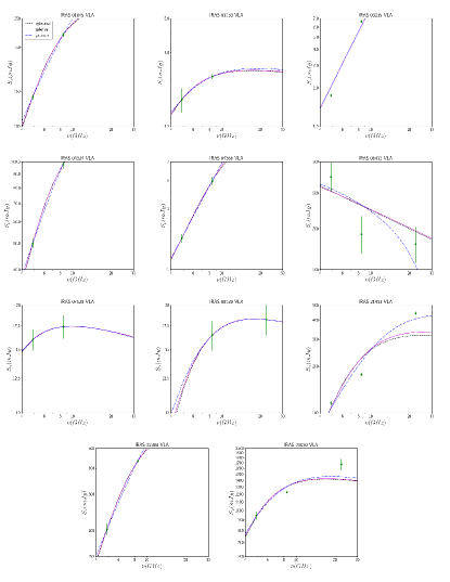
Figure 5: Fits of the three models of the IRAS sources detected at two or three wavelengths. Dots are the observational data. Dash, continuous, and dash-dot lines are for cylindrical, spherical and Gaussian models respectively. See the text for details.

Assuming an isothermal ionized gas with a temperature of 10⁴ K, we minimized equation 8 to obtain the best spectral fit for each source. H II region models were applied to 11 sources from Table 7 with a spectral index greater than $\sim-0.1$. Of these, eight were detected at two wavelengths, and three were detected at three wavelengths. The resulting best fits for each source are shown in Figure 5, and their respective physical parameters, as determined by the best fit, are listed in Table 8. However, from our two or three wavelength dataset, we were unable to accurately discriminate between specific models for the symmetry and structure of H II regions, highlighting the need for additional multi-band observations. In this way, elements such as morphology and inferred substructure from observations can help us in characterizing H II regions more accurately. For more details on each source, please refer to Appendix 0.6.

We present the results in the form of a final catalog, (see Table 9), that summarizes the calculated physical parameters for 20 sources. These were calculated from 3.6 cm emission for sources detected at a single wavelength and from H II models for sources with two or three observations. Of these sources, 17 show physical parameters consistent with those typical of ultracompact H II regions (one with cometary morphology) and 3 are compatible with being compact H II regions. Of the remaining five sources listed in Table 6, 05358-VLA1 has elongated jet-like morphology, while 05305-VLA, 06567-VLA, 21306-VLA, and 21334-VLA have a negative spectral index ($<-0.5$).

0.4.1 Detection rate of H II regions in the sample

As mentioned, the sample consists of 106 IRAS sources, 96 of which were observed at 3.6 cm and 52 at 1.3 cm, with 42 of them observed at both wavelengths. The detection rate at 3.6 cm was $\sim 25\%$ (25 sources), while at 1.3 cm it was only around 10% (five sources). There are several reasons that could account for this low detection rate, which will be explored below.

One possible reason for the low detection rate could be the poor sensitivity of the observations, which were made in snapshot mode, with integration times of 5 and 10 minutes at 3.6 and 1.3 cm, respectively. However, even with these integration times, sources with a flux density of $\sim 2$ mJy at 3.6 cm and $\sim 4$ mJy at 1.3 cm could still be detected at $3\sigma$. Thus, this factor can only account for a few cases of non-detection. On the other hand, it is also known that the lifetime of the H II regions is relatively short, which could also contribute to the low detection rate as well.

We cannot rule out the possibility that the emission measure of potential H II regions is very large ($>10^{9}$ pc cm^-6), making it optically thick at centimeter/millimeter wavelengths and resulting in a turnover frequency for optically thin emission of around 30 GHz or higher (Kurtz et al., 1994). This would mean that they cannot be detected at 3.6 cm or even at 1.3 cm. On the other hand, Sewiło et al. (2011) observed a small sample of UC and HC H II region candidates at several bands and achieved a successful detection rate with flux density ranging from 60 to 350 mJy at 1.3 and 3.6 cm, respectively. Their sources span a range of distances up to 14.0 kpc, which is close to the upper end of the range of distances in our sample. However, the large sample of sources we have explored may include some objects, especially the most compact ones, that could be affected by opacity and become undetectable, particularly at the 6 cm band. Nonetheless, as shown by Sewiło et al. (2011), this effect is not dominant, at least for the majority of H II regions observed at wavelengths above a few cm.

0.4.2 Non thermal Emission

In general, the nature of emission from astronomical sources can be classified as thermal (e.g Olnon, 1975; Reynolds, 1986) and non-thermal (e.g Deeg et al., 1993), if the spectral indices are larger than -0.1 or less than -0.5, respectively. We explore some scenarios that could explain the nature of the continuum sources with a negative spectral index.

Negative spectral indices were found in four continuum sources (05305-VLA, 06567-VLA, 21306-VLA, and 21334-VLA), with values ranging from -1.3 to -0.5, which indicate non-thermal emission. Young sources with spectral indices between $-0.5$ and $-0.1$ have been associated to gyro-synchrotron radiation, produced in strong collisions in radio jets (e.g Trinidad, Rodríguez, & Rodríguez, 2009) or in the corona of young low-mass stars (e.g Launhardt et al., 2022). Since the sample sources are related to massive star formation regions, the first scenario could be the most likely; however, strong collisions are not expected in H II regions. Spectral indices as low as $-1.2<\alpha<-0.4$ are only typically found in starburst galaxies (e.g Deeg et al., 1993).

The variability of continuum sources could also explain these negative values of the spectral index, since the observations at 3.6 and 6 cm were carried out about a decade apart. Another possibility is that the spectral index of these sources could be a result of the emission produce by two or more continuous sources. For example, for the sources IRAS 06567-VLA and IRAS 21306-VLA, there is marginal evidence that the continuous emission is not associated with a single source. In either case, to investigate the nature of these sources, new observations with higher sensitivity and angular resolution at multiple wavelengths are needed.

0.5 Conclusions

The UC H II regions are good tracers for places where early-type massive stars form, thus their study and characterization can provide important insights to understand the formation process of high-mass stars. However, due to their short lifetime, the number of known UC H II regions is relatively small. In this context, this paper is intended to increase the number of known H II regions, mainly ultra-compact, and to provide the basic data that can be used for further detailed investigations.

We conducted a study on the 1.3 and 3.6 cm continuum emission from a sample of 106 high-luminosity IRAS sources observed with the VLA in its C and B configuration, respectively. 52 sources in the sample were observed at 1.3 cm and 96 at 3.6 cm, with 42 of them observed at both wavelengths. Additionally, we used 6 cm observations reported in the literature of the detected sources. From 3.6 cm observations, we detected 25 sources, while only 5 sources were detected from the 1.3 cm observations. In general, a single radio continuum source was detected toward each IRAS region, although there is marginal evidence of double systems in some regions. We only detected two independent sources in one region.

Using the 3.6 cm emission, we performed an initial characterization of the ionized gas in all detected sources by calculating their traditional physical parameters. For sources that were also detected at 1.3 cm and those with reported 6 cm emission, we determined their spectral index and calculated models of H II regions with cylindrical, spherical, and Gaussian morphologies. Based on these results, we present a catalog of candidate H II regions detected in the sample.

0.6 Comments on Individual Sources

General information is given below for the 25 sources detected at 3.6 cm, as well as the most relevant results of the study carried out in this paper. Table 4 lists the luminosity and distance for all sources, while Table 6 gives the physical parameters calculated from the 3.6 emission. In addition, Figures 1 and 2 display the 3.6 cm contour maps, and Figure 3 shows the 1.3 cm contour maps of the detected sources in the sample. Contour maps of sources with 6 cm emission are shown in Figure 4. The physical parameters obtained from the models of the H II regions with cylindrical, spherical and Gaussian symmetry, as well as the best fits to the observational data are given in Table 8 and Figure 5, respectively.

IRAS 01045+6505 is located in the HCS 6236 molecular cloud (Snell, Carpenter & Heyer, 2002). A UC H II region, spatially coincident with a CS molecular clump, and two submillimeter sources has been detected toward it (Mookerjea, Sandell & Wouterloot, 2007). We detect 1.3 and 3.6 cm continuum emission toward IRAS 01045+6505. In the field, we observe only one compact source, which is also detected at 6 cm and coincides with the millimeter source 01045-SMM1 and the UC H II region reported by Mookerjea, Sandell & Wouterloot (2007). A spectral index, $\alpha$ $\sim$ 0.3 was estimated using the flux density of the three wavelengths. However, the flux density at 1.3 cm appears to be very low compared to those obtained at 3.6 and 6 cm, which makes the estimated spectral index unreliable. It is possible that the flux density of the source is variable with the time.

Using only the 3.6 and 6 cm flux densities, we estimated a value of $\alpha$ $\sim$ 1.3. We interpret this spectral index as a partially thick optically UC H II region, which is consistent with the interpretation given by Mookerjea, Sandell & Wouterloot (2007). No significant variations are observed in Figure 5 between the cylindrical, spherical and Gaussian geometries of the UC H II region; however, based on its morphology at 1.3 and 3.6 cm, the spherical model could be the most suitable.

IRAS 01133+6434. It was previously observed in radio continuum by Urquhart et al. (2009), finding only one radio source. In our study, we detected a single compact and spherical source in the field at 3.6 cm. However, at 6 cm, this continuum source exhibits two emission peaks, with the strongest one coinciding with the 3.6 cm emission. Using its 3.6 and 6 cm flux density, we estimated a spectral index of $\sim 0.6$, which is consistent with a partially thin optically H II region. The physical parameters obtained from the H II region’s models are given in Table 8, suggesting that it is an UC H II region sustained by a ZAMS B1 star. We did not find significant differences between the three models applied.

IRAS 03235+5808. This source has been little studied. Urquhart et al. (2009) detected a continuum source and NH₃ emission in the region. A continuum source is detected at 3.6 and 6 cm, which has a compact and spherical morphology at both wavelengths and coincides spatially with the IRAS center position. Its spectral index ($\alpha\sim 2.4$) and physical parameters suggest that it could be an optically thick UC H II region, which is confirmed by analyzing the H II region with three symmetries. The central source of the UC H II region is a ZAMS B0 star.

IRAS 04324+5106. A radio continuum source and four millimeter sources were detected in the region by Urquhart et al. (2009) and Klein, Posselt & Schreyer (2005), respectively. We observed a continuum source at 3.6 cm, that is very extended and shows a cometary morphology. This source is also detected at 6 cm with a similar morphology. Based on its spectral index between 3.6 and 6 cm ($1.2$) and applying the H II region’s models, we find the continuum source is consistent with a compact H II region with Gaussian symmetry (see Figure 5 and Table 8), which is associated with a ZAMS O9.5 star.

IRAS 04366+5022. Urquhart et al. (2009) detect a single continuum source at 6 cm, which has NH₃ emission (Urquhart et al., 2011). We detected a continuum source toward IRAS 04366+5022 at wavelengths of 3.6 and 6 cm. This source, at 3.6 cm, shows an irregular morphology with several protuberances, suggesting the presence of more than one embedded continuum source (Figure 1). However, high angular resolution observations will be necessary to confirm this speculation.

Assuming the continuum emission is produced by a single source, we estimated a spectral index of $\sim 1.9$. This value could be consistent with an optically thick H II region. Based on the H II region models, we found that its physical parameters are consistent with this assumption (see Figure 5 and Table 8).

IRAS 05305+3029. This source has been poorly studied and no ammonia or other molecular tracer has been detected in the region. A compact continuum source was detected in the field at 3.6 cm, located about $14.3^{\prime\prime}$ northeast of the IRAS position. Although it was not detected at 1.3 cm, the continuum source was detected at 6 cm. It shows a compact morphology at 3.6 cm with a protuberance observed at 6 cm, suggesting that the continuum source could be a binary system. In this way, more sensitive observations will be necessary to verify this hypothesis.

We calculated a spectral index of $\sim-1.2$, which is too negative to be credible. This value could be explained by invoking variability of the continuum source and/or the possibility that it could be a double system. The physical parameters of this continuum source, using its 3.6 cm emission, are consistent with an UC H II region harboring a ZAMS B1 star. However, simultaneous multi-wavelength observations with high angular resolutions are necessary to confirm its nature.

IRAS 05358+3543 is located toward the star cluster S233 (Yao et al., 2000) and has been studied at several wavelengths. Although it is strong at millimeter wavelengths (Beuther et al., 2002a), centimeter continuum emission has not been detected (e.g Sridharan et al., 2002). In addition, a massive bipolar outflow with a high degree of collimation has been detected (Beuther et al., 2002b).

The 3.6 cm continuum map reveals two sources in the field. The strongest source, IRAS 05358-VLA1, shows an elongated morphology in the northwest-southeast direction, while the second source, IRAS 05358-VLA2, is weaker and more compact. Although IRAS 05358-VLA1 has a jet-like morphology, it was not detected at 1.3 cm or 6 cm, then, its spectral index was not calculated. Moreover, this continuum source is not associated with the millimeter source detected by Beuther et al. (2002a) or the bipolar SiO outflow detected by Beuther et al. (2002b), whose center is about $75^{\prime\prime}$ to the southeast. Nonetheless, the elongation of the IRAS 05358-VLA1 is similar to that of the SiO bipolar outflow (northwest-southeast direction). Although IRAS 05358-VLA1 does not seem to be the driver source of the SiO outflow, there may be some relationship. Furthermore, using its 3.6 cm emission, we estimated a mass-loss rate of $\dot{M}$ = 2.71$\times$10^-10 M${}_{\sun}$ yr^-1, and a momentum rate of $\dot{P}$ = 1.35$\times$10^-7 M${}_{\sun}$ yr^-1 km s^-1, suggesting this source is a thermal jet (e.g. Anglada, Rodríguez, & Carrasco-González, 2018).

On the other hand, the derived physical parameters of the weak continuum source, IRAS 05358-VLA2, seem to be consistent with a UC H II region hosting a ZAMS B2 star.

IRAS 05553+1631 is one of the nearest regions in the sample ($\sim 1.2$ kpc; (Wouterloot & Brand, 1989)). A millimeter source was detected by Williams, Fuller, & Sridharan (2004) in the region. We detected one compact and spherical continuum source at 3.6 cm, which is offset by approximately $\sim 2.5^{\prime\prime}$ from the millimeter source. Based on its physical parameters, we suggest that it could be an UC H II region, harboring a ZAMS B3 star.

IRAS 06055+2039 is located toward S235. Six-millimeter sources and ammonia emission were observed in the region by Klein, Posselt & Schreyer (2005). We detected a weak continuum source toward the IRAS region at 3.6 cm. However, it is shifted about $\sim 49^{\prime\prime}$ from the IRAS position. Besides, this continuum source is not spatially coincident with any of the other millimeter sources detected by Klein, Posselt & Schreyer (2005), the closest one being $1^{\prime\prime}$ away. Our calculated physical parameters suggest that this compact source is a H II region with a ZAMS B2 star.

IRAS 06412–0105 is located toward the WB870 region. A millimeter source was detected in the region by Klein, Posselt & Schreyer (2005), which was interpreted as a low-mass dust core embedded into the extended emission. Contour maps at 3.6 and 1.3 cm show a source with cometary morphology that has a size of about $13^{\prime\prime}\times 11^{\prime\prime}$ at 3.6 cm and is spatially coincident with the IRAS source. A similar morphology is also observed at 6 cm, but the compact source seems to split into a double system.

Taking into account the compact and extended emission of the continuum source, we estimated a spectral index of $\sim-0.2$, which is interpreted as an optically thin H II region. In addition, H II region models indicate that this source is an UC H II region with Gaussian morphology, associated with a ZAMS O7.5 star.

IRAS 06567–0355. Both millimetre and IR sources were detected in this region by Klein, Posselt & Schreyer (2005) and Zhang & Wu (1996), respectively. NH₃ (1,1) and (2,2) emission, as well as a bipolar outflow were also reported by Klein, Posselt & Schreyer (2005) and Wu, Huang & He (1996), respectively.

We detected a nearly spherical 3.6 cm continuum source that is shifted about $\sim 290^{\prime\prime}$ from the IRAS source and is not spatially coincident with the millimeter source. In addition, this continuum source was detected at 6 cm, but with a slightly elongated morphology and showing several protuberances. Using the centimeter emission, we calculate a spectral index of $\sim-0.5$ between 3.6 and 6 cm, which is consistent with non-thermal emission. This spectral index’s value could be explain by the presence of variability in the flux density or by the fact the continuum source could be a multiple system. Simultaneous and high angular resolution observations will be necessary to confirm its nature.

IRAS 07299–1651. A millimeter and infrared sources, separated by $\sim 2.4^{\prime\prime}$, were detected by Klein, Posselt & Schreyer (2005) and Rosero et al. (2019), respectively. A single continuum source is detected at 3.6 cm in the field, but not at 1.3 cm. It is spatially coincident with the millimeter source, and based on its continuum emission, this source is consistent with an UC H II region maintained by a ZAMS B3 star.

IRAS 07311–2204 is located toward BRAN 45 region, which has a diameter of $\sim 25^{\prime}$ and CO emission (May, Alvarez, & Bronfman, 1997). We detected an extended continuum source at 3.6 cm with angular size $\sim 6^{\prime\prime}$. This continuum source is spatially coincident with the IRAS source and lies within the BRAN 45 region. Assuming it to be a H II region and based on its 3.6 cm continuum emission, we found that the ionizing star is a ZAMS B0.5 star.

IRAS 07427–2400 is a high-mass star-forming region (MacLeod et al., 1998). Trinidad (2011) found a cluster of at least three radio continuum sources, two of which are UC H II regions, while the strongest source is a jet. These sources have also been detected at millimeter wavelengths by (Qiu et al., 2009). We detected a continuum source at 3.6 cm; however, we note a peculiar morphology that resembles neither a H II region nor thermal jets. This fact could be explained due to the low angular resolution of the observations at 3.6 cm, which do not spatially separate the embedded sources detected by Trinidad (2011).

IRAS 07528–3441. Using CS(2–1) and ¹²CO observations, Bronfman, Nyman & May (1996) found an UC H II region and a molecular outflow toward IRAS 07528–3441. In addition, NH₃ (1–1) has been also detected by Urquhart et al. (2011).

The 3.6 cm continuum emission shown in Figure 2, seems to be elongated in the north-south direction, as is also observed at 6 cm. A continuum peak is clearly detected and there is evidence of a weaker second peak. However, the second peak detected at 6 cm is not coincident with the one detected at 3.6 cm. In addition, the continuum emission does not spatially coincide with the UC H II region detected by Bronfman, Nyman & May (1996), which is offset by $\sim 2^{\prime}$. Based on the spectral index ($\sim 0.15$) and the H II region models, we found that this continuum source is consistent with an UC H II region harboring a B1 ZAMS star.

IRAS 08189–3602 was observed as a radio continuum source by Wouterloot & Brand (1989), while Arnaud et al. (2015) found a compact H II region through mm and sub–mm observations. We detected a continuum source at 3.6 and 1.3 cm with a large angular size of $\sim 20^{\prime\prime}$ at 3.6 cm. A strong peak at 3.6 cm is observed, but other less defined peaks are also observed. These peaks are not probably associated with other continuum sources, but rather irregularities of extended emission. To investigate the possibility of the secondary emission peaks being associated with compact embedded sources, we made contour maps removing the shorter baselines, both 1.3 and 3.6 cm. However, no additional compact sources were detected.

Considering the 1.3 and 3.6 cm emission of the source, Figure 5 shows that the three H II region models fit very well for the data. Based on its morphology and physical parameters, we adopt the cylindrical model. However, spherical or Gaussian models can also be consistent. This UC H II region is separated by $\sim 15^{\prime\prime}$ from the compact H II region detected at mm wavelengths by Arnaud et al. (2015).

IRAS 18094–1823 (G12.20–0.03) is a high–mass star-forming region (Hill et al., 2005) and is not part of the original of the AC295 project. It is located about $\sim$ 4^′ to the west of the UC H II  region  G12.21–0.10 (e.g. de la Fuente et al., 2020a, and references therein). It stand out because the presence of low-resolution VLA emission at 3.6 cm (size $\sim$ 20^′) that coincides with IRAS 18094–1823 in the radio–continuum study for G12.21–0.10 presented by de la Fuente et al. (2018). In additon, using 6 cm observations from the CORNISH survey, Kalcheva et al. (2018) suggested that this object is a UC H II region. The 3.6 cm contour map shows a spherical compact source, whose emission is produced by a UC H II region. We found the ionizing star is a ZAMS B0 star.

IRAS 19120+1103 (G45.47+0.05) is also not included in the original sample of 104 sources, but VLA low-resolution emission at 3.6 cm was detected in a study by de la Fuente et al. (2020a). Its continuum emission is more associated with the UC H II region with extended emission G45.45+0.06 (see de la Fuente et al., 2020a, and references therein). This source was confirmed as a star-forming region by the detection of H₂O and OH maser emission by Kim, Kim, & Kim (2019). It was classified as an irregular UC H II region base on its 6 cm emission (Wood & Churchwell, 1989). The physical parameters and morphology of the 3.6 cm emission are consistent with a compact H II region, with the central source being a ZAMS O9.5 star.

IRAS 21306+5540 is located toward S128, which has been studied at radio wavelengths by Ho, Haschick, & Israel (1981) and Fich (1986). Three compact H II regions were found by Ho, Haschick, & Israel (1981), labeled as S128A, S128B, and S128N with exciting stars O6, O6, and O9.5, respectively. In addition, an IR and submillimeter source have been detected by (Umana et al., 2008), and the presence of a bipolar outflow in the east-west direction has been reported by (Kim, Kim, & Kim, 2015).

We detected a nearly compact continuum source at 3.6 cm, with a protuberance toward the north. This compact source was also detected at 6 cm and coincides with the source S128N detected by Ho, Haschick, & Israel (1981). We estimated a spectral index is about $\sim-1.1$, which is interpreted as non-thermal emission. Such negative spectral indices are generally associated with extra-galactic sources. However, this continuum source is embedded in a star-forming region and has been catalogued as compact H II region. We could explain this spectral index due to the variability of the source or to the fact that the continuum emission is not associated with a single source (e.g., a protuberance can be observed at 3.6 cm). Its physical parameters are reported in Table 6, assuming it is a H II region.

IRAS 21334+5039. A compact H II region, with a ZAMS B0 star, was discovered in this region through radio continuum observations by McCutcheon et al. (1991), which coincides with NH₃ emission detected by Urquhart et al. (2011). In addition, Obonyo et al. (2019) searched non-thermal radio emission toward this region, but the results were negative.

We detected one continuum source in the field at 3.6 cm, with a compact spherical morphology. A similar morphology was also observed at 6 cm. However, this source has a offset $\sim 60^{\prime\prime}$ from the compact H II region detected by McCutcheon et al. (1991). We determined a spectral index about $-0.55$, which could indicate a non-thermal nature or variability of the source (observations were carried out with a separation of about ten years). Further simultaneous observations will be necessary to determine its nature.

IRAS 21413+5442. Two radio continuum sources have been detected by Miralles, Rodríguez & Scalise (1994) and classified as a compact H II and a UC H II region, respectively. In addition, IR observations by Anandarao et al. (2008) show the presence of a stellar cluster.

We detected a source in the field at 6, 3.6 and 1.3 cm. The morphology of the source is compact, showing slight protrusions in all three wavelengths. It coincides with the IRAS source and one of the IR sources detected by Anandarao et al. (2008), which was interpreted as a massive young stellar object. However, this continuum source is offset by about $20^{\prime}$ from the H II regions reported by Miralles, Rodríguez & Scalise (1994). Using the 1.3, 3.6 and 6 cm flux densities, we obtained a spectral index of 0.85, suggesting this source is a partial thick optically H II region. By modeling this continuum source as H II region, we find that its physical parameters are consistent with a UC H II region with Gaussian morphology harboring a ZAMS O8 star.

IRAS 22134+5834. NH₃ and water maser emission were detected toward the IRAS region by Sunada et al. (2007). We detected a continuum source at 3.6 cm, located about $3.5^{\prime\prime}$ from the IRAS source. This source shows a compact spherical morphology, and based on its derived physical parameters from the 3.6 cm emission, it could be classified as an UC H II region with a ZAMS B1 star.

IRAS 22308+5812 is located toward Sh2–138 (Wouterloot & Brand, 1989). A compact H II region was studied by Martín-Hernández et al. (2002) and NH₃ (1,1) emission was reported by Urquhart et al. (2011).

We detected a continuum source at 3.6 cm with a cometary-like H II region morphology, with its emission peak about $2^{\prime\prime}$ of the IRAS source. A similar morphology was also observed at 6 cm. Based on its spectral index ($\sim 1.4$), physical parameters and morphology observed in Figure 2, we suggest this source is a UC H II region with a ZAMS O7.5 star and Gaussian distribution (see Figure 5).

IRAS 23030+5958 is located toward S156 (Lee, Murray, & Rahman, 2012) and it is one of the most luminous regions of the sample. Using low angular resolution observations at 6 cm, Israel (1977) found a group of H II regions (S156) with at least two O stars and three B stars.

We detected continuum emission at 3.6 and 1.3 cm, but the morphology does not have a well–defined structure; rather it shows a complicated morphology with at least three continuum peaks detected at both wavelengths (VLA1, VLA2, and VLA3), aligned in the east-west direction. This morphology is also observed at 6 cm. All continuum peaks are contained in the S156A source and interpreted as a H II region. In general, the morphology of S156A and the other sources detected by Israel (1977) was explained by the quasi-stationary blister type model. Considering that all the emission detected in the field is part of a single H II region and based on its spectral index information and derived physical parameters, we found that its continuum emission is consistent with a partial optically thin UC H II region excited by ZAMS O8 stars.

6

Table 1: Physical Parameters of H II regionsa.

Type of H II	Size	EM	ne	M${}_{\rm\hbox{H{ }{II}{ }}}$	Referenceb
region	(pc)	(cm-6 pc)	(cm-3)	(M⊙)
Hypercompact	$\sim$ 0.003	$\gtrsim$ 1010	$\gtrsim$ 106	$\sim$ 10-3	1
Ultracompact	$\lesssim$ 0.1	$\gtrsim$ 107	$\gtrsim$ 104	$\sim$ 10-3	2,3
Compact	$\lesssim$ 0.5	$\gtrsim$ 107	$\gtrsim$ 5$\times$103	$\sim$ 1	4
Ultracompact with	1–20	104–105	$\gtrsim$ 102-103	5–103	5
Extended Emission
aAdapted from Kurtz & Franco (2002); de la Fuente et al. (2020b) b1.- Sewiło et al. (2008, 2004), 2.- Wood & Churchwell (1989), 3.- Kurtz et al. (1994), 4.- Lumsden et al. (2013), 5.- (de la Fuente et al., 2020a, b, and references therein).

-2cm-2cm

Table 2: The sample of 106 IRAS sources: 96 observed at 3.6 cm, 10 at 1.3 cm, and 42 observed at both wavelengths.

9 IRAS RA (J2000) DEC (J2000) IRAS RA (J2000) DEC (J2000) IRAS RA (J2000) DEC (J2000) Source (h:m:s) ($\circ$: $\prime$: $\prime\prime$ ) Source (h:m:s) ($\circ$: $\prime$: $\prime\prime$ ) Source (h:m:s) ($\circ$: $\prime$: $\prime\prime$ ) 00117+6412* 00:14:27.72 64:28:46.3 05554+2013 05:58:24.56 20:13:57.5 07528-3441 07:54:49.97 -34:49:45.9 00338+6312** 00:36:47.51 63:29:02.1 06055+2039* 06:08:32.82 20:39:16.2 07530-3436** 07:54:56.18 -34:49:38.3 00412+6638* 00:44:15.23 66:54:40.6 06073+1249* 06:10:12.43 12:48:45.5 08007-2829 08:02:46.36 -28:25:47.4 00468+6508 00:49:55.82 65:43:38.7 06084+1727 06:11:24.52 17:26:26.5 08008-3423 08:02:42.30 -34:31:46.8 00468+6527** 00:49:55.82 65:43:38.7 06089+1727** 06:11:44.41 17:26:05.1 08088-3554* 08:10:43.49 -36:03:29.8 00556+6048 00:58:40.13 61:04:44.0 06103+1523 06:13:18.21 15:23:16.1 08140-3556 08:15:58.98 -36:08:20.0 00578+6233 01:00:55.81 62:49:28.5 06104+1524A** 06:13:21.32 15:23:56.9 08159-3543 08:17:52.89 -35:52:49.9 01045+6505* 01:07:50.70 65:21:21.4 06105+1756* 06:13:28.33 17:55:29.5 08189-3602* 08:20:47.86 -36:12:34.4 01133+6434* 01:16:37.39 64:50:38.8 06114+1745* 06:14:23.69 17:44:36.5 08212-4146 08:23:02.96 -41:55:48.5 02044+6031* 02:08:05.05 60:45:56.7 06155+2319A 06:18:35.15 23:18:11.4 08245-4038* 08:26:17.70 -40:48:35.1 02395+6244 02:43:28.72 62:57:05.3 06208+0957* 06:23:34.41 09:56:22.1 08274-4111 08:29:13.94 -41:10:44.4 02437+6145* 02:47:40.43 61:58:26.3 06306+0437* 06:33:16.36 04:34:56.8 18094–1823a 18:12:23.63 -18:22:53.7 02455+6034 02:49:23.23 60:47:01.2 06331+1102 06:35:56.01 11:00:17.5 19120+1103b 19:14:25.67 11:09:26.0 02461+6147 02:50:08.11 61:59:47.1 06337+1051 06:36:29.48 10:49:05.1 21074+4949 21:09:08.09 50:01:59.8 03233+5809** 03:27:22.33 58:19:45.8 06381+1039 06:40:58.00 10:36:48.8 21080+4950 21:09:42.83 50:08:29.5 03235+5808* 03:27:31.15 58:19:21.3 06412-0105* 06:43:44.97 -01:08:06.7 21202+5157* 21:21:53.18 52:10:43.6 04034+5107 04:07:11.93 51:24:44.7 06426+0025 06:45:15.50 00:22:25.9 21290+5535 21:30:38.70 55:48:59.6 04324+5102 04:36:16.08 51:08:12.8 06446+0029 06:47:12.87 00:26:06.5 21306+4927** 21:05:15.62 49:40:01.2 04324+5106* 04:36:19.70 51:12:44.6 06501+0143 06:52:45.57 01:40:14.9 21306+5540* 21:32:11.56 55:53:23.7 04366+5022* 04:40:26.12 50:28:24.7 06547-0109A 06:57:16.69 -01:13:39.5 21334+5039* 21:35:09.18 50:53:09.2 04547+4753* 04:58:29.66 47:58:27.6 06567-0355* 06:59:15.76 -03:59:39.0 21334+5329 21:35:05.86 53:43:01.2 04579+4703 05:01:39.74 47:07:23.1 06570-0401 06:59:30.95 -04:05:35.1 21407+5441* 21:42:23.68 54:55:06.7 05100+3723 05:13:25.43 37:27:04.5 07024-1102 07:04:45.65 -11:07:14.5 21413+5442* 21:43:01.36 54:56:16.3 05271+3059 05:30:21.22 31:01:27.2 07069-1045 07:04:45.65 -11:07:14.5 22134+5834* 22:15:09.08 58:49:09.3 05274+3345* 05:30:45.62 33:47:51.6 07061-0414* 07:08:38.75 -04:19:07.5 22308+5812* 22 32 46.01 58 28 21.8 05281+3412 05:31:26.60 34:14:57.7 07207-1435 07:23:01.28 -14:41:32.5 22475+5939* 22:49:29.47 59:54:56.6 05305+3029* 05:33:44.81 30:31:04.5 07295-1915** 07:33:10.45 -19:28:42.9 22502+5944** 22:51:59.86 59:59:16.9 05334+3149 05:36:41.08 31:51:13.8 07298-1919 07:32:02.46 -19:26:02.3 22506+5944* 22:52:38.63 60:00:55.8 05358+3543* 05:39:10.39 35:45:19.2 07299-1651* 07:32:10.00 -16:58:14.7 22539+5758 22:56:00.01 58:14:45.9 05361+3539 05:39:27.66 35:40:43.0 07333-1838 07:35:34.31 -18:45:32.5 22551+6139 22:57:11.23 61:56:03.4 05375+3536 05:40:52.52 35:38:23.8 07334-1842 07:35:40.95 -18:48:59.0 22570+5912* 22:59:06.50 59:28:27.7 05375+3540* 05:40:53.64 35:42:15.7 07422-2001 07:44:27.85 -20:08:31.9 23030+5958* 23:05:10.62 60:14:40.4 05490+2658 05:52:12.93 26:59:32.9 07427-2400* 07:44:51.90 -24:07:40.6 23033+5951 23:05:25.16 60:08:11.6 05480+2545* 05:51:10.75 25:46:14.3 07311-2204* 07:33:20.24 -22:10:57.7 23139+5939 23:16:09.32 59:55:22.8 05553+1631* 05:58:13.87 16:32:00.1 07434-2044 07:45:35.47 -20:51:38.6 23151+5912 23:17:21.09 59:28:48.8 23545+6508** 23:57:05.23 65:25:10.8 *Sources observed at 3.6 and 1.3 cm at high resolution. **Sources observed at 1.3 cm at high resolution. aSource refereed as 18094–G12.20. Low resolution at 3.6 cm observation only. See text for details. bSource refereed as 19120–G45.47. Arguable designation: the IRAS source is more related with G45.45+0.06. Low resolution at 3.6 cm only. See text for details.

4

Table 3: Phase calibrator’s observational parameters.

Calibrator	RA (J2000)	DEC (J2000)	3.6 Bootstrapped Flux Density
	(h:m:s)	($\circ$: $\prime$: $\prime\prime$ )	(Jy)
2023+544	20h23m55.844s	54∘27′35.83′′	1.12$\pm$0.01
2230+697	22h30m36.470s	69∘46′28.08′′	0.44$\pm$0.01
0228+673	02h28m50.051s	67∘21′03.03′′	0.78$\pm$0.02
0359+509	03h59m29.747s	50∘57′50.16′′	1.47$\pm$0.03
0555+398	05h55m30.806s	39∘48′49.17′′	4.86$\pm$0.08
0530+135	05h30m56.417s	13∘31′55.15′′	1.40$\pm$0.02
0700+171	07h00m01.525s	17∘09′21.70′′	1.11$\pm$0.01
0725–009	07h25m50.640s	00∘54′56.54′′	0.95$\pm$0.01
0730–116	07h30m19.112s	–11∘41′12.60′′	4.63$\pm$0.05
0828–375	08h28m04.780s	–37∘31′06.28′′	1.07$\pm$0.01

6

Table 4: Sources detected at 3.6 cm

IRASa	VLA 3.6 cm	RA (J2000)	Dec (J2000)	Distanceb	LFIRb
Source	Source	(h:m:s)	($\circ$: $\prime$: $\prime\prime$ )	(kpc)	(104L⊙)
01045+6505	01045–VLA	01:07:51.34	65:21:22.4	10.71	8.0017
01133+6434	01133–VLA	01:16:36.67	64:50:42.4	4.12	0.842
03235+5808	03235–VLA	03:27:31.34	58:19:21.7	4.22	1.302
04324+5106	04324–VLA	04:36:21.03	51:12:54.7	5.83	6.003
04366+5022	04366–VLA	04:40:27.20	50:28:29.2	5.93	3.003
05305+3029	05305–VLA	05:33:45.83	30:31:18.0	10.44	0.604
05358+3543	05358–VLA1	05:39:15.62	35:46:42.1	1.85	0.665
	05358–VLA2	05:39:15.13	35:46:41.6	1.85	0.665
05553+1631	05553–VLA	05:58:13.53	16:31:58.4	1.23	0.203
06055+2039	06055–VLA	06:08:35.44	20:39:03.5	2.93	3.003
06412–0105	06412–VLA	06:43:48.42	-01:08:20.5	7.13	9.003
06567–0355	06567–VLA	06:59:15.74	-03:59:36.8	2.36	1.8018
07299–1651	07299–VLA	07:32:09.79	-16:58:12.2	1.43	0.703
07311–2204	07311–VLA	07:33:19.92	-22:10:57.5	8.07	20.007
07427–2400	07427–VLA	07:44:52.03	-24:07:42.1	6.93	50.1019
07528–3441	07528–VLA	07:54:56.12	-34:49:37.8	1.28	20.008
08189–3602	08189–VLA	08:20:54.92	-36:13:02.5	7.63	30.0020
18094–1823c	18094–G12.20	18:12:23.63	-18:22:53.7	14.013	86.8014
19120+1103d	19120–G45.47	19:14:25.67	11:09:26.0	8.415	49.216
21306+5540	21306–VLA	21:32:11.76	55:53:40.9	3.79	1.103
21334+5039	21334–VLA	21:35:11.13	50:52:13.1	5.010	2.1010
21413+5442	21413–VLA	21:43:01.47	54:56:18.0	7.911	1.4511
22134+5834	22134–VLA	22:15:09.25	58:49:08.9	2.33	1.343
22308+5812	22308–VLA	22:32:45.62	58:28:18.2	5.73	9.003
23030+5958	23030–VLA	23:05:10.20	60:14:47.2	4.412	10.003
aThe observed source does not necessary coincides with the IRAS source. bThe distance and the FIR luminosity are from the IRAS region, and not necessary corresponds to the observed sources at 3.6 cm. Values taken from: 1.- Rudolph De Geus & Wouterloot (1996), 2.- Maud et al. (2015), 3.- Wouterloot & Brand (1989), 4.- Lumsden et al. (2013), 5.- Lu et al. (2014), 6.- Tapia et al. (1997), 7.- May, Alvarez, & Bronfman (1997), 8.- Preite–Martínez (1988), 9.- Kim, Kim, & Kim (2015), 10.- McCutcheon et al. (1991), 11.- Navarrete et al. (2015), 12.- Lee, Murray, & Rahman (2012), 13.- Hill et al. (2005), 14.- We assume the IRAS FIR luminosity of G12.21–0.10 (de la Fuente et al., 2018, 2020a), 15.- Wu et al. (2019), 16.- We assume the IRAS FIR luminosity of G45.45+0.06 (de la Fuente et al., 2020a), 17.- Snell, Carpenter & Heyer (2002), 18.- Klein, Posselt & Schreyer (2005), 19.- MacLeod et al. (1998), 20.- Arnaud et al. (2015). cThis source was not included in the original sample of 94 sources (see Table 3). dThis source was not included in the original sample of 94 sources (see Table 3). The nearest IRAS source is 19120+1103, but this coincide in position with the UC H II region with extended emission G45.455+0.058 or G45.45+0.06 (de la Fuente et al., 2020a). See text for discussion. The distance is adopted from Wu et al. (2019).

7

Table 5: Observational parameters of the sources detected at 1.3, 3.6, and 6.0 cm

VLA 3.6 cm	$\lambda$	Sν	Beam Size	PA	RMS Noise	Size
Source	(cm)	(mJy)	( ” $\times$ ” )	(deg)	(mJy beam-1)	( ” $\times$ ” )
01045–VLA	6.0	140.4$\pm$4.2	1.57$\times$1.05	134	0.25	3.13$\times$2.91
	3.6	289.8$\pm$6.7	1.57$\times$1.05	120	0.41	3.10$\times$2.92
	1.3	100.5$\pm$5.4	1.57$\times$1.05	27	0.67	3.12$\times$3.00
01133–VLA	6.0	1.5$\pm$0.3	1.61$\times$1.07	168	0.06	3.11$\times$1.73
	3.6	2.1$\pm$0.1	1.61$\times$1.07	129	0.06	1.75$\times$1.15
03235–VLA	6.0	1.7$\pm$0.1	1.41$\times$1.10	146	0.03	1.50$\times$1.13
	3.6	6.6$\pm$0.2	1.41$\times$1.10	144	0.07	1.48$\times$1.16
04324–VLA	6.0	50.0$\pm$2.1	1.34$\times$1.08	47	0.06	8.82$\times$7.27
	3.6	97.7$\pm$3.3	1.34$\times$1.08	46	0.12	8.85$\times$8.31
04366–VLA	6.0	1.8$\pm$0.1	1.30$\times$1.08	141	0.03	2.41$\times$1.73
	3.6	5.0$\pm$0.4	1.30$\times$1.08	158	0.03	2.72$\times$2.27
05305–VLA	6.0	0.4$\pm$0.1	1.26$\times$1.15	146	0.02	1.32$\times$1.15
	3.6	0.21$\pm$0.01	1.26$\times$1.15	120	0.02	1.30$\times$1.21
05358–VLA1	3.6	1.8$\pm$ 0.2	0.88$\times$0.74	139	0.02	3.04$\times$1.05
05358–VLA2	3.6	0.8$\pm$ 0.1	0.88$\times$0.74	30	0.02	2.35$\times$1.49
05553–VLA	3.6	0.8$\pm$0.1	1.00$\times$0.62	135	0.03	1.11$\times$0.82
06055–VLA	3.6	0.8$\pm$0.1	1.11$\times$0.74	124	0.09	1.30$\times$0.82
06412–VLA	6.0	850.0$\pm$47.0	1.51$\times$1.25	57	0.67	13.85$\times$12.17
	3.6	685.0$\pm$48.0	1.51$\times$1.25	62	0.90	12.97$\times$10.74
	1.3	660.0$\pm$44.0	1.51$\times$1.25	146	1.90	12.59$\times$12.36
06567–VLA	6.0	49.3$\pm$3.2	1.69$\times$1.24	161	0.21	4.58$\times$3.65
	3.6	37.0$\pm$1.1	1.69$\times$1.24	166	0.07	3.68$\times$3.53
07299–VLA	3.6	0.26$\pm$0.01	1.40$\times$0.76	148	0.01	1.44$\times$0.86
07311–VLA	3.6	4.0$\pm$0.3	1.50$\times$0.76	165	0.01	6.26$\times$5.28
07427–VLA	3.6	2.3$\pm$0.2	1.65$\times$0.77	160	0.02	1.81$\times$0.95
07528–VLA	6.0	16.0$\pm$1.1	4.52$\times$1.14	153	0.08	5.57$\times$3.30
	3.6	17.4$\pm$1.3	4.52$\times$1.14	163	0.12	6.08$\times$2.85
08189–VLA	3.6	16.5$\pm$1.6	4.24$\times$1.17	176	2.72	26.66$\times$16.20
	1.3	18.2$\pm$1.8	4.24$\times$1.17	179	2.45	19.43$\times$10.77
18094–G12.20	3.6	7.2$\pm$0.1	12.54$\times$7.26	167	0.15	12.84$\times$7.31
19120–G45.47	3.6	112.4$\pm$1.7	8.23$\times$7.64	159	1.34	8.34$\times$7.63
21306–VLA	6.0	74.0$\pm$3.3	1.81$\times$1.14	116	0.46	3.87$\times$3.37
	3.6	39.9$\pm$2.6	1.81$\times$1.14	128	0.40	3.35$\times$2.76
21334–VLA	6.0	7.7$\pm$0.1	1.80$\times$1.15	93	0.12	1.82$\times$1.21
	3.6	5.7$\pm$0.1	1.80$\times$1.15	93	0.06	1.84$\times$1.17
21413–VLA	6.0	115.7$\pm$3.7	1.87$\times$1.13	93	0.29	2.18$\times$1.40
	3.6	177.1$\pm$4.4	1.87$\times$1.13	91	0.73	2.13$\times$1.32
	1.3	441.8$\pm$9.8	1.87$\times$1.13	90	1.89	2.04$\times$1.24
22134–VLA	3.6	4.7$\pm$0.3	0.82$\times$0.72	116	0.20	0.98$\times$0.84
22308–VLA	6.0	203.0$\pm$13.0	1.90$\times$1.07	86	0.47	7.66$\times$5.02
	3.6	433.0$\pm$25.0	1.90$\times$1.07	79	1.14	7.67$\times$5.07
23030–VLA	6.0	945.0$\pm$44.0	1.62$\times$1.19	95	1.40	14.79$\times$7.50
	3.6	1226.0$\pm$72.0	1.62$\times$1.19	90	2.52	12.79$\times$5.52
	1.3	1670.0$\pm$110.0	1.62$\times$1.19	96	5.86	12.19$\times$5.65

8

Table 6: Physical Parameters of the sources using their 3.6 cm continuum emission

VLA 3.6 cm	Size	EM	ne	M${}_{\hbox{H{ }{II}{ }}}$	Ni	Spectral	H II regiona
Source	(pc)	(106cm-6 pc)	(103cm-3)	(M⊙)	(s-1)	Type	Type
01045–VLA	0.16	21.30	11.68	0.5792	48.39	O8	C
01133–VLA	0.03	0.67	4.80	0.0015	45.41	B1	UC
03235–VLA	0.03	2.54	9.72	0.0025	45.93	B0.5	UC
04324–VLA	0.24	0.88	1.91	0.3501	47.38	B0	C
04366–VLA	0.07	0.53	2.71	0.0129	46.10	B0.5	UC
05305–VLA	0.06	0.09	1.18	0.0039	45.22	B1	UC
05358–VLA1b	0.02	0.29	4.03	0.0003	44.64	B2	UC
05358–VLA2	0.02	0.14	2.92	0.0002	44.27	B2	UC
05553–VLA	0.01	0.57	10.08	0.00002	43.93	B3	UC
06055–VLA	0.01	0.47	5.61	0.0002	44.69	B2	UC
06412–VLA	0.41	3.24	2.82	2.4979	48.40	O8	C
06567–VLA	0.04	1.89	6.85	0.0058	46.16	B0.5	UC
07299–VLA	0.01	0.13	4.10	0.00003	43.57	B3	UC
07311–VLA	0.22	0.08	0.60	0.0873	46.27	B0.5	C
07427–VLA	0.05	0.82	4.21	0.0054	45.91	B0.5	UC
07528–VLA	0.03	0.58	4.72	0.0011	45.26	B1	UC
08189–VLA	0.79	0.02	0.17	1.1159	46.84	B0	UC
18094–G12.20	0.68	0.05	0.26	1.0963	47.02	B0	UC
19120–G45.47	0.33	1.17	1.90	0.8519	47.76	O9.5	C
21306–VLA	0.05	2.84	7.19	0.0155	46.60	B0.5	UC
21334–VLA	0.04	1.66	6.74	0.0043	46.02	B0.5	UC
21413–VLA	0.07	39.41	24.39	0.0924	47.91	O9.5	UC
22134–VLA	0.01	3.78	19.30	0.0003	45.26	B1	UC
22308–VLA	0.18	7.10	6.35	0.4514	48.01	O9	C
23030–VLA	0.20	9.73	7.06	0.6858	48.24	O8.5	C
aUC = UC H II region and C = Compact H II region. bThis source has an elongated, jet-like morphology. See Appendix 0.6.

7

Table 7: Spectral Index of the sources detected at two and/or three wavelengths

VLA 3.6 cm	Wavelength	Spectral
Source	(cm)	Index
01045–VLA	3.6 & 6	1.3$\pm$0.2
01133–VLA	3.6 & 6	0.6$\pm$0.8
03235–VLA	3.6 & 6	2.4$\pm$0.2
04324–VLA	3.6 & 6	1.2$\pm$0.2
04366–VLA	3.6 & 6	1.9$\pm$0.5
05305–VLA	3.6 & 6	–1.2$\pm$0.5
06412–VLA	1.3, 3.6 & 6	–0.2$\pm$0.4
06567–VLA	3.6 & 6	–0.5$\pm$0.3
07528–VLA	3.6 & 6	0.2$\pm$0.4
08189–VLA	1.3 & 3.6	0.1$\pm$0.3
21306–VLA	3.6 & 6	–1.1$\pm$0.3
21334–VLA	3.6 & 6	–0.6$\pm$0.1
21413–VLA	1.3, 3.6 & 6	0.9$\pm$0.2
22308–VLA	3.6 & 6	1.4$\pm$0.4
23030–VLA	1.3, 3.6 & 6	0.4$\pm$0.3

7

Table 8: Physical Parameters: H II Region Models

VLA 3.6 cm	Sizea	EM	ne	Ni	Spectral	Morphology	H II b
Source	(pc)	$cm^{-6}$ pc	$cm^{-3}$	(s-1)	Type		Type
01045-VLA	0.16	4.39$\times$108	8.92$\times 10^{4}$	6.25$\times 10^{48}$	O6.5	Spherical	UC
01133-VLA	0.03	1.60$\times$108	2.51$\times 10^{5}$	4.80$\times 10^{45}$	B1	Spherical	UC
03235-VLA	0.03	6.68$\times$109	1.63$\times 10^{6}$	1.97$\times 10^{47}$	B0	Spherical	UC
04324-VLA	0.24	4.67$\times$108	3.87$\times 10^{5}$	6.11$\times 10^{47}$	O9.5	Gaussian	C
04366-VLA	0.07	1.37$\times$109	6.41$\times 10^{5}$	7.06$\times 10^{46}$	B0	Spherical	UC
06412-VLA	0.41	1.19$\times$106	2.88$\times 10^{3}$	3.26$\times 10^{48}$	O7.5	Gaussian	UCc
07528-VLA	0.03	3.59$\times$107	1.02$\times 10^{5}$	1.96$\times 10^{45}$	B1	Cylindrical	UC
08189-VLA	0.79	1.71$\times$108	1.16$\times 10^{5}$	1.30$\times 10^{47}$	B0	Spherical	UC
21413-VLA	0.07	5.75$\times$108	3.10$\times 10^{5}$	2.76$\times 10^{48}$	O8	Gaussian	UC
22308-VLA	0.18	9.14$\times$108	4.04$\times 10^{5}$	3.85$\times 10^{48}$	O7.5	Gaussian	UC
23030-VLA	0.20	1.07$\times$108	8.85$\times 10^{4}$	2.67$\times 10^{48}$	O8	Gaussian	UC
aTaken from the 3.6 cm RC emission b UC = UC H II region and C = Compact H II region. c UC with cometary morphology

7

Table 9: Final catalog of H II regionsa

IRAS	VLA 3.6 cm	Size	Size	EM	ne	M${}_{\rm\hbox{H{ }{II}{ }}}$	H II a
Source	Source	(arcsec)	(pc)	(106cm-6 pc)	(103cm-3)	(M⊙)	Type
01045+6505	01045–VLA	3.02	0.16	21.30	11.68	0.5792	UC
01133+6434	01133–VLA	0.83	0.03	0.67	4.80	0.0015	UC
03235+5808	03235–VLA	0.87	0.03	2.54	9.72	0.0025	UC
04324+5106	04324–VLA	8.56	0.24	0.88	1.91	0.3501	C
04366+5022	04366–VLA	2.30	0.07	0.53	2.71	0.0129	UC
05358+3543	05358–VLA2	1.84	0.02	0.14	2.92	0.0003	UC
05553+1631	05553–VLA	0.95	0.01	0.57	10.08	0.00002	UC
06055+2039	06055–VLA	0.95	0.01	0.47	5.61	0.0002	UC
06412–0105	06412–VLA	0.41	3.24	1.19	2.82	2.4979	UCb
07299–1651	07299–VLA	1.11	0.01	0.13	4.10	0.00003	UC
07311–2204	07311–VLA	5.75	0.22	0.08	0.60	0.0873	C
07427–2400	07427–VLA	1.31	0.05	0.82	4.21	0.0054	UC
07528–3441	07528–VLA	3.78	0.03	0.58	4.72	0.0011	UC
08189–3602	08189–VLA	3.48	0.79	0.02	0.17	1.1159	UC
18094–1823	18094–G12.20	2.10	0.68	0.05	0.26	1.0963	UC
19120–1103	19120–G45.47	2.20	0.33	1.17	1.90	0.8519	C
21413+5442	21413–VLA	1.70	0.07	39.41	24.39	0.0924	UC
22134+5834	22134–VLA	0.91	0.01	3.78	19.30	0.0003	UC
22308+5812	22308–VLA	6.24	0.18	7.10	6.35	0.4514	UC
23030+5958	23030–VLA	4.30	0.20	9.73	7.06	0.6858	UC
a UC = UC H II region and C = Compact H II region. b UC with cometary morphology

References

- Anandarao et al. (2008) Anandarao, B. G., Venkata, R. V., Ghosh, S. K., Ojha, D. K., Kumar, M. S. N., 2008, MNRAS, 390, 1185
- Anglada, Rodríguez, & Carrasco-González (2018) Anglada, G., Rodríguez, L. F., Carrasco–González, C., 2018, Astron. Astrophys Rev. 26, 3
- Arnaud et al. (2015) Arnaud, M., Atrio–Barandela, F., Aumont, J., et al., 2015, A&A, 573, 6
- Beuther et al. (2002a) Beuther, H., Sridharan, T. K., Schilke, P., Menten, K. M., Wyrowski, F., 2002a, ApJ, 566, 945
- Beuther et al. (2002b) Beuther, H., Schilke, P., Gueth, F., McCaughrean, M., Andersen, M., Sridharan, T. K., Menten, K. M., 2002b, A&A387, 931
- Beuther et al. (2007) Beuther, H., Churchwell, E. B., McKee, C. F., Tan, J. C., 2007, In Protostars and Planets V, ed. B. Reipurth, D. Jewitt, & K. Keil, 165–180
- Bronfman, Nyman & May (1996) Bronfman, L., Nyman, L.-A., May, J., 1996, A&AS, 115, 81
- Deeg et al. (1993) Deeg, H.-J., Brinks, E., Duric, N., Klein, U., Skillman, E. D., 1993, ApJ, 410, 626
- de la Fuente et al. (2020a) de la Fuente, E., Porras, A., Trinidad, M. A., Kurtz, S. E., Kemp, S. N., Tafoya, D., Franco, J., Rodríguez-Rico, C., 2020a, MNRAS, 492, 895
- de la Fuente et al. (2020b) de la Fuente, E., Tafoya, D., Trinidad, M. A., Porras, A., Nigoche-Netro, A., Kemp, S. N., Kurtz, S. E., Franco, J., Rodríguez-Rico, C. A., 2020b, MNRAS, 497, 4436
- de la Fuente et al. (2018) de la Fuente, E., Trinidad, M. A., Porras, A., Rodríguez-Rico, C., Araya, E. D., Kurtz, S., Hofner, P., Nigoche-Netro, A., 2018, RMxAA, 54, 129
- De Pree, Rodriguez, & Goss (1995) De Pree, C. G., Rodriguez, L. F., Goss, W. M., 1995, RMxAA, 31, 39
- Fich (1986) Fich, M., 1986, AJ, 92, 787
- Franco et al. (2001) Franco, J., Kurtz, S. E., García-Barreto, J. A., García-Segura, G., de la Fuente, E., Hofner, P., Esquivel A., 2001, Astrophysics and Space Science Supplement, 277, 71
- Franco et al. (2000a) Franco, J., García-Barreto, J. A., de la Fuente, E., 2000a, ApJ, 544, 277
- Franco et al. (2000b) Franco, J., Kurtz, S., Hofner, P., Testi, L., García-Segura, G., Martos, M, 2000b, ApJ, 542, 143
- Franco, Tenorio-Tagle, and Bodenheimer (1990) Franco, J., Tenorio-Tagle, G., Bodenheimer, P., 1990, ApJ, 349, 126
- Garay & Lizano (1999) Garay, G., Lizano, S., 1999, PASP, 111, 1049
- Hill et al. (2005) Hill T., Burton, M. G., Minier, V., 2005, MNRAS, 366, 405
- Ho, Haschick, & Israel (1981) Ho, P. T. P., Haschick, A. D., Israel, F. P., 1981, ApJ, 243, 526
- Israel (1977) Israel, F. P., 1977, A&A, 59, 27
- Jaffe & Martin-Pintado (1999) Jaffe, D. T., Martin-Pintado, J., 1999, ApJ, 520, 162
- Kalcheva et al. (2018) Kalcheva, I. E., Hoare, M. G., Urquhart, J. S., Kurtz, S., Lumsden, S. L., Purcell, C. R., Zijlstra, A. A., 2018, A&A, 615, A103
- Kim, Kim, & Kim (2015) Kim, K. T., Kim, W. J., Kim, C. H., 2015, JKAS., 48, 365
- Kim, Kim, & Kim (2019) Kim, W. J., Kim, K. T., Kim, K. T., 2019, ApJS, 244 2
- Kurtz & Franco (2002) Kurtz, S., Franco ,J., 2002, RMxAA Conf. Ser, 12, 16
- Kurtz et al. (1994) Kurtz, S., Churchwell, E., Wood, D. O. S., 1994, ApJS, 91, 659
- Klein, Posselt & Schreyer (2005) Klein, R., Posselt, B., Schreyer, K., 2005, ApJS, 161, 361
- Launhardt et al. (2022) Launhardt, R., Loinard, L., Dzib, S. A., Forbrich, J., Bower, G. C., Henning, T. K., Mioduszewski, A. J., Reffert, S., 2022, ApJ, 931, 43
- Lee, Murray, & Rahman (2012) Lee, E. J., Murray, N., Rahman, M., 2012, ApJ, 752, 146
- Lu et al. (2014) Lu, X., Zhang, Q., Liu, H. B., Wang, J., Gu, Q., 2014, ApJ, 790, 84
- Lumsden et al. (2013) Lumsden, S. L., Hoare, M. G., Urquhart, J. S., Oudmaijer, R. D., Davies, B., Mottram, J. C., Cooper, H. D. B., Moore, T. J. T., 2013, ApJS, 208, 11
- MacLeod et al. (1998) MacLeod, G, C., Scalise, E. Jr., Saedt, S., Galt, J. A., Gaylard, M. J., 1998, AJ, 116, 1897.
- Martín-Hernández et al. (2002) Martín-Hernández, N. L., Peeters, E., Morisset, C., Tielens, A. G. G. M., Cox, P., Roelfsema, P. R., Baluteau, J. -P., Schaerer, D., Mathis, J. S., Damour, F., Churchwell, E., Kessler, M. F., 2002, A&A, 381, 606
- Maud et al. (2015) Maud, L. T., Moore, T. J. T., Lumsden, S. L., Mottram, J. C., Urquhart, J. S., Hoare, M. G., 2015, MNRAS, 453, 645
- May, Alvarez, & Bronfman (1997) May, J., Alvarez, H., Bronfman, L., 1997, A&A, 327, 325
- McCutcheon et al. (1991) McCutcheon, W. H., Dewdney, P. E., Purton, R., Sato, T., 1991, AJ, 101, 1435
- McMullin et al. (2007) McMullin, J. P., Waters, B., Schiebel, D., Young, W., Golap, K., 2007, Astronomical Data Analysis Software and Systems XVI, 376, 127
- Miralles, Rodríguez & Scalise (1994) Miralles, M. P., Rodríguez, L. F., Scalise, E., 1994, ApJS, 92, 173
- Motte, Bontemps & Louvet (2018) Motte, F., Bontemps, S., Louvet, F., 2018, ARA&A, 56, 41
- Mookerjea, Sandell & Wouterloot (2007) Mookerjea, B., Sandell, G., Wouterloot, J. G. A., 2007, A&A, 473, 485
- Navarrete et al. (2015) Navarrete F., Damineli A., Barbosa C. L., Blum, R. D, 2015, MNRAS, 450, 4364
- Obonyo et al. (2019) Obonyo, W. O., Lumsden, S. L., Hoare, M. G., Purser, S. J. D., Kurtz, S. E., Johnston, K. G., 2019, MNRAS, 486, 3664
- Olnon (1975) Olnon, F. M., 1975, A&A, 39, 217
- Panagia (1973) Panagia, N., 1973, AJ, 78, 929
- Phillips (2007) Phillips, J. P., 2007, MNRAS, 380, 369
- Phillips (2008) Phillips, J. P., 2008, New Astronomy, 13, 60
- Preite–Martínez (1988) Preite–Martínez, A., 1988, A&AS, 76, 317
- Qiu et al. (2009) Qiu, K., Zhang, Q., Wu, J., Chen, H-R, 2009, ApJ, 696, 66
- Reynolds (1986) Reynolds, S. P., 1986, ApJ, 304, 713
- Rodríguez et al. (2012) Rodríguez, L. F., González, R. F., Montes, G. Asiri, H. M., Raga, A., Cantó, J., 2012, ApJ, 755, 152
- Rosero et al. (2019) Rosero, V., Tanaka, K. E. I., Tan, J. C., Marvil, J., 2019, ApJ, 873, 20
- Rudolph De Geus & Wouterloot (1996) Rudolph, A. L., Brand, J., De Geus, E. J., Wouterloot, J. G. A., 1996, ApJ, 458, 653
- Schraml & Mezger (1969) Schraml, J., Mezger, P. G., 1969, ApJ, 156, 269
- Sewiło et al. (2011) Sewiło, M., Churchwell, E., Kurtz, S., Goss, W. M., Hofner, P., 2011, ApJS, 194, 44
- Sewiło et al. (2008) Sewiło M., Churchwell, E., Kurtz, S., Goss, W. M., Hofner, P., 2008, ApJ, 681, 350
- Sewiło et al. (2004) Sewiło, M., Churchwell, E., Kurtz, S., Goss, W. M., Hofner, P., 2004, ApJ, 605, 285
- Snell, Carpenter & Heyer (2002) Snell, R. L., Carpenter, J. M., Heyer, M. H., 2002, ApJ, 578, 229
- Sunada et al. (2007) Sunada, K., Nakazato, T., Ikeda, N., Hongo, S., Kitamura, Y., Yang, J., 2007, PASJ, 59, 1185
- Sridharan et al. (2002) Sridharan, T. K., Beuther, H., Schilke, P., Menten, K. M., Wyrowski, F., 2002, ApJ, 566, 931
- Tapia et al. (1997) Tapia, M., Persi, P., Bohigas, J., Ferrari-Toniolo, M., 1997, AJ, 113, 1769
- Trinidad et al. (2003) Trinidad, M. A., Curiel, S., Cantó, J., D’Alessio, P., Rodríguez, L. F., Torrelles, J. M., Gómez, J. F., Patel, N., Ho, P. T. P., 2003, ApJ, 589, 386
- Trinidad, Rodríguez, & Rodríguez (2009) Trinidad, M. A., Rodríguez, T., Rodríguez, L. F., 2009, ApJ, 706, 244
- Trinidad (2011) Trinidad, M. A., 2011, AJ, 142, 6
- Umana et al. (2008) Umana, G., Leto, P., Trigilio, C., Buemi, C. S., Manzitto, P., Toscano, S., Dolei, S., Cerrigone, L., 2008, A&A, 482, 529
- Urquhart et al. (2009) Urquhart, J. S., Hoare, M. G., Purcell, C. R., Lumsden, S. L., Oudmaijer, R. D., Moore, T. J. T., Busfield, A. L., Mottram, J. C., Davies, B., 2009, A&A, 501, 539
- Urquhart et al. (2011) Urquhart, J. S., Morgan, L. K., Figura, C. C., Moore, T. J. T., Lumsden, S. L., Hoare, M. G., Oudmaijer, R. D., Mottram, J. C., Davies, B., Dunham, M. K., 2011, MNRAS, 418, 1689
- Williams, Fuller, & Sridharan (2004) Williams, S. J., Fuller, G. A., Sridharan, T. K., 2004, A&A, 417, 115
- Wood & Churchwell (1989) Wood, D.O.S., Churchwell, E., 1989, ApJS, 69, 831
- Wouterloot & Brand (1989) Wouterloot, J. G. A., Brand, J., 1989, A&AS, 80, 149
- Wu et al. (2019) Wu, Y. W., Reid, M. J., Sakai, N., Dame, T. M., Menten, K. M., Brunthaler, A., Xu, Y., Li, J. J., Ho, B., Zhang, B., Rygl, K. L. J., Zheng, X. W., 2019, ApJ, 874, 94
- Wu, Huang & He (1996) Wu, Y., Huang, M., He, J., 1996, A&AS, 115, 283
- Yao et al. (2000) Yao, Y., Ishii, M., Nagata, T., Nakaya, H., Sato, S., 2000, ApJ, 542, 392
- Zhang & Wu (1996) Zhang, W.-H., Wu, Y.-F., 1996, CAA, 20, 326
6