A Mini-Neptune Orbiting the Metal-poor K Dwarf BD+29 2654

Fei Dai fdai@caltech.edu NASA Sagan Fellow Division of Geological and Planetary Sciences, 1200 E California Blvd, Pasadena, CA, 91125, USA Department of Astronomy, California Institute of Technology, Pasadena, CA 91125, USA Kevin C. Schlaufman William H. Miller III Department of Physics and Astronomy, Johns Hopkins University, 3400 N Charles St, Baltimore, MD 21218, USA Henrique Reggiani The Observatories of the Carnegie Institution for Science, 813 Santa Barbara St, Pasadena, CA 91101, USA Luke Bouma 51 Pegasi b Fellow Department of Astronomy, California Institute of Technology, Pasadena, CA 91125, USA Andrew W. Howard Department of Astronomy, California Institute of Technology, Pasadena, CA 91125, USA Ashley Chontos Department of Astrophysical Sciences, Princeton University, 4 Ivy Lane, Princeton, NJ 08540, USA Henry Norris Russell Fellow Institute for Astronomy, University of Hawai‘i, 2680 Woodlawn Drive, Honolulu, HI 96822, USA Daria Pidhorodetska Department of Earth and Planetary Sciences, University of California, Riverside, CA 92521, USA Judah Van Zandt Department of Physics & Astronomy, University of California Los Angeles, Los Angeles, CA 90095, USA Joseph M. Akana Murphy NSF Graduate Research Fellow Department of Astronomy and Astrophysics, University of California, Santa Cruz, CA 95064, USA Ryan A. Rubenzahl NSF Graduate Research Fellow Department of Astronomy, California Institute of Technology, Pasadena, CA 91125, USA Alex S. Polanski Department of Physics and Astronomy, University of Kansas, Lawrence, KS 66045, USA Jack Lubin Department of Physics & Astronomy, University of California Irvine, Irvine, CA 92697, USA Corey Beard Department of Physics & Astronomy, University of California Irvine, Irvine, CA 92697, USA Steven Giacalone Department of Astronomy, University of California Berkeley, Berkeley, CA 94720, USA Rae Holcomb Department of Physics & Astronomy, University of California Irvine, Irvine, CA 92697, USA Natalie M. Batalha Department of Astronomy and Astrophysics, University of California, Santa Cruz, CA 95060, USA Ian Crossfield Department of Physics and Astronomy, University of Kansas, Lawrence, KS, USA Courtney Dressing 501 Campbell Hall, University of California at Berkeley, Berkeley, CA 94720, USA Benjamin Fulton NASA Exoplanet Science Institute/Caltech-IPAC, MC 314-6, 1200 E California Blvd, Pasadena, CA 91125, USA Daniel Huber Institute for Astronomy, University of Hawai‘i, 2680 Woodlawn Drive, Honolulu, HI 96822, USA Sydney Institute for Astronomy, School of Physics, University of Sydney NSW 2006, Australia Howard Isaacson 501 Campbell Hall, University of California at Berkeley, Berkeley, CA 94720, USA Centre for Astrophysics, University of Southern Queensland, Toowoomba, QLD, Australia Stephen R. Kane Department of Earth and Planetary Sciences, University of California, Riverside, CA 92521, USA Erik A. Petigura Department of Physics & Astronomy, University of California Los Angeles, Los Angeles, CA 90095, USA Paul Robertson Department of Physics & Astronomy, University of California Irvine, Irvine, CA 92697, USA Lauren M. Weiss Department of Physics and Astronomy, University of Notre Dame, Notre Dame, IN 46556, USA Alexander A. Belinski Sternberg Astronomical Institute Lomonosov Moscow State University 119992, Moscow, Russia, Universitetskii prospekt Andrew W. Boyle Department of Astronomy, California Institute of Technology, 1200 E. California Blvd, Pasadena, CA 91125 USA Christopher J. Burke Department of Physics and Kavli Institute for Astrophysics and Space Research, Massachusetts Institute of Technology, Cambridge, MA 02139, USA Amadeo Castro-González Centro de Astrobiología (CAB, CSIC-INTA), Depto. de Astrofísica, ESAC campus, 28692, Villanueva de la Cañada (Madrid), Spain David R. Ciardi Caltech/IPAC-NASA Exoplanet Science Institute, 770 S. Wilson Avenue, Pasadena, CA 91106, USA Tansu Daylan Department of Astrophysical Sciences, Princeton University, Princeton, NJ 08544, USA LSSTC Catalyst Fellow Akihiko Fukui Komaba Institute for Science, The University of Tokyo, 3-8-1 Komaba, Meguro, Tokyo 153-8902, Japan Instituto de Astrofísica de Canarias (IAC), 38205 La Laguna, Tenerife, Spain Holden Gill Department of Astronomy, University of California Berkeley, Berkeley, CA 94720, USA Natalia M. Guerrero Department of Astronomy, University of Florida, Gainesville, FL, 32611, USA Department of Physics and Kavli Institute for Astrophysics and Space Research, Massachusetts Institute of Technology, Cambridge, MA 02139, USA Coel Hellier Astrophysics Group, Keele University, Staffordshire ST5 5BG, U.K Steve B. Howell NASA Ames Research Center, Moffett Field, CA 94035, USA Jorge Lillo-Box Centro de Astrobiología (CAB, CSIC-INTA), Depto. de Astrofísica, ESAC campus, 28692, Villanueva de la Cañada (Madrid), Spain Felipe Murgas Instituto de Astrofísica de Canarias (IAC), Calle Vía Láctea s/n, 38205 La Laguna, Tenerife, Spain Departamento de Astrofísica, Universidad de La Laguna (ULL), E-38206 La Laguna, Tenerife, Spain Norio Narita Komaba Institute for Science, The University of Tokyo, 3-8-1 Komaba, Meguro, Tokyo 153-8902, Japan Astrobiology Center, 2-21-1 Osawa, Mitaka, Tokyo 181-8588, Japan Instituto de Astrofísica de Canarias (IAC), 38205 La Laguna, Tenerife, Spain Enric Pallé Instituto de Astrofísica de Canarias (IAC), Calle Vía Láctea s/n, 38205 La Laguna, Tenerife, Spain David R. Rodriguez Space Telescope Science Institute, 3700 San Martin Drive, Baltimore, MD, 21218, USA Arjun B. Savel Department of Astronomy, University of Maryland, College Park, College Park, MD 20742 USA Avi Shporer Department of Physics and Kavli Institute for Astrophysics and Space Research, Massachusetts Institute of Technology, Cambridge, MA 02139, USA Keivan G. Stassun Department of Physics and Astronomy, Vanderbilt University, Nashville, TN 37235, USA Stephanie Striegel SETI Institute, 339 N Bernardo Ave Suite 200, Mountain View, CA 94043, USA NASA Ames Research Center, Moffett Field, CA 94035, USA Douglas A. Caldwell NASA Ames Research Center, Moffett Field, CA 94035, USA Jon M. Jenkins NASA Ames Research Center, Moffett Field, CA 94035, USA George R. Ricker Department of Physics and Kavli Institute for Astrophysics and Space Research, Massachusetts Institute of Technology, Cambridge, MA 02139, USA Sara Seager Department of Physics and Kavli Institute for Astrophysics and Space Research, Massachusetts Institute of Technology, Cambridge, MA 02139, USA Department of Earth, Atmospheric and Planetary Sciences, Massachusetts Institute of Technology, Cambridge, MA 02139, USA Department of Aeronautics and Astronautics, MIT, 77 Massachusetts Avenue, Cambridge, MA 02139, USA Roland Vanderspek Department of Physics and Kavli Institute for Astrophysics and Space Research, Massachusetts Institute of Technology, Cambridge, MA 02139, USA Joshua N. Winn Department of Astrophysical Sciences, Princeton University, 4 Ivy Lane, Princeton, NJ 08544, USA

(Received ?; Revised ?; Accepted ?)

Abstract

We report the discovery and Doppler mass measurement of a 7.4-day 2.3- $R_{\oplus}$ mini-Neptune around a metal-poor K dwarf BD+29 2654 (TOI-2018). Based on a high-resolution Keck/HIRES spectrum, the Gaia parallax, and multi-wavelength photometry from the ultraviolet to the mid-infrared, we found that the host star has $T_{\text{eff}}=4174^{+34}_{-42}$ K, $\log{g}=4.62^{+0.02}_{-0.03}$ , $[\text{Fe/H}]=-0.58\pm 0.18$ , $M_{\ast}=0.57\pm 0.02~{}M_{\odot}$ , and $R_{\ast}=0.62\pm 0.01~{}R_{\odot}$ . Precise Doppler measurements with Keck/HIRES revealed a planetary mass of $M_{\text{p}}=9.2\pm 2.1~{}M_{\oplus}$ for TOI-2018 b. TOI-2018 b has a mass and radius that are consistent with an Earth-like core with a $\sim 1\%$ -by-mass hydrogen/helium envelope, or an ice-rock mixture. The mass of TOI-2018 b is close to the threshold for run-away accretion and hence giant planet formation. Such a threshold is predicted to be around 10 $M_{\oplus}$ or lower for a low-metallicity (low-opacity) environment. If TOI-2018 b is a planetary core that failed to undergo run-away accretion, it may underline the reason why giant planets are rare around low-metallicity host stars (one possibility is their shorter disk lifetimes). With a K-band magnitude of 7.1, TOI-2018 b may be a suitable target for transmission spectroscopy with the James Webb Space Telescope. The system is also amenable to metastable Helium observation; the detection of a Helium exosphere would help distinguish between a H/He enveloped planet and a water world.

planets and satellites: composition; planets and satellites: formation; planets and satellites: interiors

^†^†journal: AAS^†^†software: AstroImage (Collins et al., 2017), Isoclassify (Huber et al., 2017),isochrones (Morton, 2015) MIST (Choi et al., 2016b), SpecMatch-Syn (Petigura, 2015), Batman (Kreidberg, 2015), emcee (Foreman-Mackey et al., 2013), iSpec (Blanco-Cuaresma et al., 2014; Blanco-Cuaresma, 2019), colte (Casagrande et al., 2021)^†^†facilities: Keck:I (HIRES), TESS,MuSCAT2, WASP, Palomar, Lick, Gemini, Carlo ALto, Caucasian Observatory of Sternberg Astronomical Institute

1 Introduction

The occurrence rate of giant planets is strongly correlated with the host star metallicity (Gonzalez, 1997; Santos et al., 2004; Fischer & Valenti, 2005). This strong correlation has been regarded as supporting evidence for the core accretion theory of planet formation (Pollack et al., 1996). In a metal-rich disk, a high abundance of solid materials helps planet embryos grow quickly to the critical mass that initiates run-away gas accretion and gas giant formation. On the other hand, the close-in, sub-Neptune planets (<1AU, 1-4 $R_{\oplus}$ , also known as the Kepler-like planets) are much more common around solar-type stars compared to giant planets (e.g. Howard et al., 2012; Petigura et al., 2013; Fressin et al., 2013). The occurrence rate of sub-Neptune planets also has a much weaker dependence on host metallicity compared to the giant planets (e.g. Wang & Fischer, 2015; Petigura et al., 2018). One might argue that the formation of gas giant planets may be a threshold-crossing event that has to occur when the gaseous disk is still present. On the other hand, the formation of sub-Neptune planets is less demanding on core assembly rate and can proceed in low-metallicity environments. The super-Earths planets may not accrete a substantial envelope (Rogers, 2015), whereas the mini-Neptunes only acquire their envelopes towards the final vestige of the disk when the disk starts to become optically thin (Lee & Chiang, 2016; Lee et al., 2018).

So far, most planet occurrence studies (e.g. Kepler Borucki et al., 2011) are based on surveys of stars with sun-like metallicities [Fe/H] between $-0.5$ and $0.5$ . It is not clear how the occurrence-metallicity correlation extends to a more metal-depleted regime ([Fe/H] $<-0.5$ ). The standard minimum mass solar nebula (Hayashi, 1981) has about 30 $M_{\oplus}$ of solid materials within the innermost 1 AU for the in-situ formation of the close-in sub-Neptune planets. The total amount of solid materials would decrease to 3-9 $M_{\oplus}$ for -1<[Fe/H]<-0.5. Such a limited supply of solids may prevent the formation of multiple close-in sub-Neptune planets.

To further investigate the influence of host metallicity, we (Schlaufman et al., in prep) are studying the occurrence rate of transiting sub-Neptune planets around metal-poor (-1<[Fe/H]<-0.5) stars observed as the TESS mission (Ricker et al., 2014). Thanks to the nearly full-sky coverage of TESS, we were able to cross-match the TESS Input Catalog (Stassun et al., 2019) with ground-based spectroscopic surveys, including the Large Sky Area Multi-Object Fiber Spectroscopic Telescope (LAMOST) Low-Resolution Survey (LRS) Data Release (DR) 6 (Cui et al., 2012), the Radial Velocity Experiment (RAVE) DR6 (Steinmetz et al., 2020), and the GALactic Archaeology with Hermes (GALAH) DR3 (Buder et al., 2021). We identified a sample of about 10,000 dwarf stars with -1<[Fe/H]<-0.5. We have carried out a systematic search for transiting planets among this sample. This search led to the discovery of BD+29 2654, which was also discovered independently by the TESS team as TOI-2018 (Guerrero et al., 2021). TOI-2018 is a bright, nearby K-dwarf among our transiting planet hosts that is particularly amenable to follow-up observations. We also present an additional transiting signal, TOI-2018.02, which was not reported by the TESS team (Guerrero et al., 2021) due to its lower signal-to-noise ratio (SNR). We carried out a detailed characterization of the host star and Doppler mass measurements of the planets to help the community plan follow-up observations of this system.

The paper is organized as follows. Section 2 presents a detailed characterization of the host star TOI-2018 with particular attention to its metallicity. Section 3 describes our transit detection and modeling of this system based on the light curves. In Section 4, we present the radial velocity (RV) measurements of TOI-2018 and the resultant constraints on the planetary masses. Section 5 discusses the implications of our findings.

2 Stellar Properties

2.1 Fundamental and Photospheric Parameters

To derive the stellar parameters, we analyzed an archival high-resolution, high-SNR spectra of TOI-2018 taken with the High Resolution Echelle Spectrometer on the 10-meter Keck Telescope (Keck/HIRES, Vogt et al., 1994) on Jul 26 2012. The spectrum was taken without the iodine-cell and reached an SNR of about 200 per reduced pixel near 5500Å after a 600-sec exposure. We made use of both spectroscopy and isochrones to infer the photospheric and fundamental stellar parameters as described in Reggiani et al. (2022). Isochrones are especially useful for determining the effective temperature $T_{\text{eff}}$ of the star, because high-quality multi-wavelength photometry from the ultraviolet to the red optical is available. Similarly, the availability of the Gaia DR3 parallax-based distance of TOI-2018 makes the calculation of surface gravity $\log{g}$ via isochrones more straightforward than it has traditionally been. With good constraints on both $T_{\text{eff}}$ and $\log{g}$ from isochrone fitting, the equivalent widths of iron lines can be used to determine metallicity $[\text{Fe/H}]$ and microturbulence $\xi$ by minimizing the dependence of individual line-based iron abundance inferences on their reduced equivalent width.

Table 1: Adopted Stellar Parameters

Property	Value	Unit
SDSS DR13 $u$	$13.385\pm 0.0264$	AB mag
Gaia DR2 DR2 $G$	$9.720\pm 0.002$	Vega mag
2MASS $J$	$7.844\pm 0.021$	Vega mag
2MASS $H$	$7.255\pm 0.020$	Vega mag
2MASS $K$	$7.104\pm 0.017$	Vega mag
WISE W1	$6.984\pm 0.062$	Vega mag
WISE W2	$7.071\pm 0.020$	Vega mag
Gaia DR3 parallax	$35.666\pm 0.014$	mas
Spectroscopically inferred parameters
$[\text{Fe/H}]$	$-0.58\pm 0.18$
$v$ sin $i$	$<2$	km s^-1
$S_{HK}$	$0.92\pm 0.03$
log $R_{\rm HK}^{\prime}$	-4.75 $\pm$ 0.04
Isochrone-inferred parameters
Effective temperature $T_{\text{eff}}$	$4174^{+34}_{-42}$	K
Surface gravity $\log{g}$	$4.62^{+0.02}_{-0.03}$	cm s^-2
Stellar mass $M_{\ast}$	$0.57\pm 0.02$	$M_{\odot}$
Stellar radius $R_{\ast}$	$0.62\pm 0.01$	$R_{\odot}$
Luminosity $L_{\ast}$	$0.10\pm 0.01$	$L_{\odot}$
Distance	$28.038\pm 0.011$	pc

Note. — Substantial systematic uncertainties may exist between different isochronal models (Tayar et al., 2022).

The inputs to our photospheric and fundamental stellar parameter inference are the equivalent widths of Fe I and Fe II atomic absorption lines, multiwavelength photometry, the Gaia parallax, and an extinction estimate. Using atomic absorption line data from Yana Galarza et al. (2019) for lines that are relatively insensitive to stellar activity (Meléndez et al., 2014), we measured the equivalent widths by fitting Gaussian profiles with the splot task in IRAF to our continuum-normalized spectrum. We also confirmed our splot equivalent widths by remeasuring the lines using iSpec (Blanco-Cuaresma et al., 2014; Blanco-Cuaresma, 2019). We only compared the clean (unblended) lines with our splot measurements and we concluded that there were no substantial differences in the EWs measured with splot and iSpec. For the blended lines we used the deblend task to disentangle absorption lines from adjacent spectral features. We gathered $u$ photometry and their uncertainties from SDSS DR13 (Albareti et al., 2017), $G$ photometry and its uncertainty from Gaia DR2 (Gaia Collaboration et al., 2016, 2018; Arenou et al., 2018; Evans et al., 2018; Hambly et al., 2018; Riello et al., 2018), $J$ , $H$ , and $Ks$ from 2MASS, and $W1$ and $W2$ from WISE. We use the Gaia DR3 parallax and its uncertainty (Gaia Collaboration et al., 2022; Fabricius et al., 2021; Lindegren et al., 2021a, b; Torra et al., 2021) as well as an extinction $A_{V}$ inference based on three-dimensional (3D) maps of extinction in the solar neighborhood from the STructuring by Inversion the Local Interstellar Medium (Stilism) program (Lallement et al., 2014, 2018; Capitanio et al., 2017). We assume Asplund et al. (2021) solar abundances. To derive the stellar parameters, we use the isochrones package by Morton (2015) to fit the MESA Isochrones and Stellar Tracks (MIST, e.g. Choi et al., 2016a; Paxton et al., 2011, 2013, 2015) to the photospheric parameters as well as the multiwavelength photometry, parallax, and extinction using the nested sampling code MultiNest (Feroz et al., 2009, 2013). We present the stellar parameters in Table 1. We would like to remind the readers that the stellar parameters derived from isochrone models are often subject to substantial systematic uncertainties between different isochrone model (e.g. 4% in stellar radius, Tayar et al., 2022). These are not explicitly included in the reported values here. As an additional check we inferred $T_{\text{eff}}$ of TOI-2018 using the colte code¹¹1https://github.com/casaluca/colte (Casagrande et al., 2021) that estimates $T_{\text{eff}}$ using a combination of color– $T_{\text{eff}}$ relations obtained by implementing the InfraRed Flux Method for Gaia and 2MASS photometry. As required by colte, we used Gaia DR3 $G$ , $G_{\text{BP}}$ , and $G_{\text{RP}}$ plus 2MASS $J$ , $H$ , and $K_{s}$ photometry as input. We find a colte-based $T_{\text{eff}}=4160\pm 81$ K, consistent with our isochrone-inferred effective temperature. We could not measure the rotational broadening $v$ sin $i$ of the host star given the resolution of our HIRES spectrum. The $v$ sin $i$ is likely smaller than 2 km s^-1 (this is consistent with the $23.5$ -day rotation period we determined in Section 3).

2.2 Chemical Abundances

To infer the elemental abundances, we first measured the equivalent widths of atomic absorption lines of Na I, Mg I, Al I, Si I, K I, Ca I, Sc II, Ti I, Ti II, V I, Cr I, Fe I, Fe II, Ni I, Co I, Y II, and Ba II in our continuum-normalized spectrum by fitting Gaussian profiles with iSpec. We avoid blended lines, and only kept lines with EWs smaller than 170 mÅ. We assume Asplund et al. (2021) solar abundances and local thermodynamic equilibrium (LTE) and used the 1D plane-parallel solar-composition MARCS model atmospheres (Gustafsson et al., 2008) and the 2019 version of MOOG (Sneden, 1973; Sneden et al., 2012) to infer elemental abundances based on each equivalent width measurement. We report our adopted atomic data, equivalent width measurements, and individual line-based abundance inferences in Table 2. We report our abundance inferences in three common systems: $A(\text{X})$ , $[\text{X/H}]$ , and $[\text{X/Fe}]$ . The abundance $A(\text{X})$ is defined $A(\text{X})=\log{N_{\text{X}}/N_{\text{H}}}+12$ , the abundance ratio $[\text{X/H}]$ is defined as $[\text{X/H}]=A(\text{X})-A(\text{X})_{\odot}$ , and the abundance ratio $[\text{X/Fe}]$ is defined as $[\text{X/Fe}]=[\text{X/H}]-[\text{Fe/H}]$ . We define the uncertainty in the abundance ratio $\sigma_{[\text{X/H}]}$ as the standard deviation of the individual line-based abundance inferences $\sigma_{[\text{X/H}]}^{\prime}$ divided by $\sqrt{n_{\text{X}}}$ where n is the number of lines used. We define the uncertainty $\sigma_{[\text{X/Fe}]}$ as the square root of the sum of squares of $\sigma_{[\text{X/H}]}$ and $\sigma_{[\text{Fe/H}]}$ . The results are reported in Tab. 3.

Table 2: Atomic data, Equivalent Widths and line Abundances. Full version online.

Wavelength	Species	Excitation Potential	log( $gf$ )	EW	$\log_{\epsilon}(\rm{X})$
(Å)		(eV)		(mÅ)
$4751.822$	NaI I	$2.104$	$-2.078$	$41.30$	$5.824$
$6154.225$	NaI I	$2.102$	$-1.547$	$82.90$	$5.721$
$6160.747$	NaI I	$2.104$	$-1.246$	$95.30$	$5.528$
$4730.029$	MgI I	$4.346$	$-2.347$	$110.30$	$7.475$
$5711.088$	MgI I	$4.346$	$-1.724$	$116.30$	$7.004$
$6318.717$	MgI I	$5.108$	$-2.103$	$37.60$	$7.498$
$4512.268$	CaI I	$2.526$	$-1.900$	$63.50$	$5.617$
$5260.387$	CaI I	$2.521$	$-1.719$	$71.70$	$5.650$
$5512.980$	CaI I	$2.933$	$-0.464$	$167.10$	$5.462$
$5867.562$	CaI I	$2.933$	$-1.570$	$64.40$	$5.771$
$6166.439$	CaI I	$2.521$	$-1.142$	$126.30$	$5.352$

Note. — This table is published in its entirety in the machine-readable format. A portion is shown here for guidance regarding its form and content.

Table 3: Elemental Abundances

Species	$A(\text{X})$	[X/H]	$\sigma_{\text{[X/H]}}$	[X/Fe]	$\sigma_{[\text{X/Fe}]}$	$n$
LTE abundances
Na I	$5.691$	$-0.529$	$0.123$	$0.051$	$0.089$	$3$
Mg I	$7.326$	$-0.224$	$0.228$	$0.356$	$0.169$	$3$
Al I	$5.796$	$-0.634$	$0.031$	$-0.054$	$0.032$	$2$
Si I	$7.230$	$-0.280$	$0.246$	$0.300$	$0.260$	$2$
Ca I	$5.570$	$-0.730$	$0.147$	$-0.150$	$0.077$	$5$
Sc I	$2.622$	$-0.518$	$0.207$	$0.062$	$0.151$	$3$
Ti II	$4.624$	$-0.346$	$0.194$	$0.234$	$0.099$	$7$
V I	$3.543$	$-0.357$	$0.281$	$0.223$	$0.120$	$7$
Cr II	$4.951$	$-0.669$	$0.000$	$-0.089$	$0.120$	$1$
Fe I	$6.880$	$-0.580$	$0.171$	$\cdots$	$\cdots$	$70$
Fe II	$6.963$	$-0.497$	$0.082$	$\cdots$	$\cdots$	$4$
Co I	$4.724$	$-0.216$	$0.185$	$0.364$	$0.087$	$6$
Ni I	$5.947$	$-0.253$	$0.307$	$0.327$	t $0.105$	$13$
Cu I	$4.035$	$-0.144$	$0.062$	$0.436$	$0.059$	$4$
Y II	$1.260$	$-0.950$	$0.000$	$-0.370$	$0.033$	$1$
Ba II	$1.519$	$-0.751$	$0.001$	$-0.171$	$0.025$	$2$

2.3 Age, SED, Thick Disk membership

To check on the system age, we measured a stellar rotation period of $23.5\pm 1.0$ days in the WASP light curve of TOI-2018 using the Lomb-Scargle periodogram (Lomb, 1976; Scargle, 1982); auto-correlation function (McQuillan et al., 2014) gives a consistent result. The rotation period translates to a gyrochronological age of 1.6 $\pm$ 0.1 Gyr according to the scaling relation of Mamajek & Hillenbrand (2008). If we use the more up-to-date empirical relations of Bouma et al. (2023), TOI-2018’s rotation period indicates an age of $2.4\pm 0.2$ Gyr. We also analyzed the chromospheric activity as seen in the Ca II H&K lines of our HIRES spectrum. We found activity indicator $S_{HK}$ = $0.92\pm 0.03$ and log $R_{\rm HK}^{\prime}$ =-4.75 $\pm$ 0.04 using the method of Isaacson & Fischer (2010). The activity level of TOI-2018 is at about 50% percentile (see Fig. 1) of stars with similar B-V color (within 0.1 in B-V) observed by the California Planet Search (Howard et al., 2010). In addition, we looked for Lithium absorption in our HIRES spectrum of TOI-2018. We could not detect a Lithium feature that is statistically significant above the nearby continuum. We note that both the strength of Lithium absorption and log $R_{\rm HK}^{\prime}$ are likely correlated with host star metallicity [Fe/H]. The existing samples are dominated by solar-metallicity stars. If TOI-2018 is indeed a thick-disk star as we will discuss shortly, one might expect it to be old ( $>$ 8-9 Gyr). A previous work by Martig et al. (2015), however, reported a curious sample of young, $\alpha$ -enhanced stars in the solar neighborhood. Given the quality and discrepancy of the various age indicators, we are unable to provide a precise age constraint on TOI-2018 as is often the case for late-type stars.

We further examined the kinematics of TOI-2018. The proper motion of TOI-2018 does not fit any known comoving associations reported in Banyan- $\Sigma$ (Gagné et al., 2018) and in Bouma et al. (2022). We also computed the Galactic UVW velocity of TOI-2018 (U,V,W = -59.6, 11.4, -8.9 km s^-1.). Using the framework of Bensby et al. (2014), TOI-2018 has a 3.1% chance of being in the thick disk based on its kinematics alone.

We also investigated the $\alpha$ -element enhancement of TOI-2018. Using Mg, Si, and Ti abundances as a proxy for the $\alpha$ elements (we excluded Ca due to its association with stellar activity), we obtained a [ $\alpha$ /Fe] = 0.29 $\pm 0.12$ . In Fig. 2, we plot the [ $\alpha$ /Fe] against [Fe/H] for TOI-2018 and a cross-match between the GALAH survey (e.g. Buder et al., 2021) and the TESS Input Catalog (Stassun et al., 2019) as presented in Carrillo et al. (2020). The $\alpha$ -element enhancement of TOI-2018 does favor a thick disk membership. However, this claim needs to be further confirmed with more precise [ $\alpha$ /Fe] and kinematic constraints.

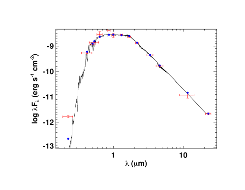
We fitted the Spectral Energy Distribution (SED) of TOI-2018 following the method of Stassun & Torres (2016). We fitted Kurucz stellar atmosphere models (Kurucz, 1979) to various photometric bands. Our fit yielded a reduced $\chi^{2}$ of 1.1. We obtained a stellar mass and radius of $0.59\pm 0.04M_{\odot}$ and $0.62\pm 0.02R_{\odot}$ which are consistent with our isochronal analysis. We did not find any evidence for an infrared excess that may be attributable to a debris disk (Fig. 3).

2.4 High Resolution Imaging

As part of our standard process for validating transiting exoplanets, and to assess the contamination of bound or unbound companions on the derived planetary radii (Ciardi et al., 2015), we observed TOI-2018 with high-resolution imaging. The star was observed with Palomar/PHARO (Hayward et al., 2001), Lick/ShARCS (Kupke et al., 2012; Gavel et al., 2014; McGurk et al., 2014), Gemini-N/Alopeke (Howell et al., 2011), Caucasian Observatory of Sternberg Astronomical Institute/Speckle Polarimeter (Safonov et al., 2017), and Carlo Alto/AstraLux (Hormuth et al., 2008) thanks to the efforts of the TESS Follow-up Observing Program (TFOP) Working Group.

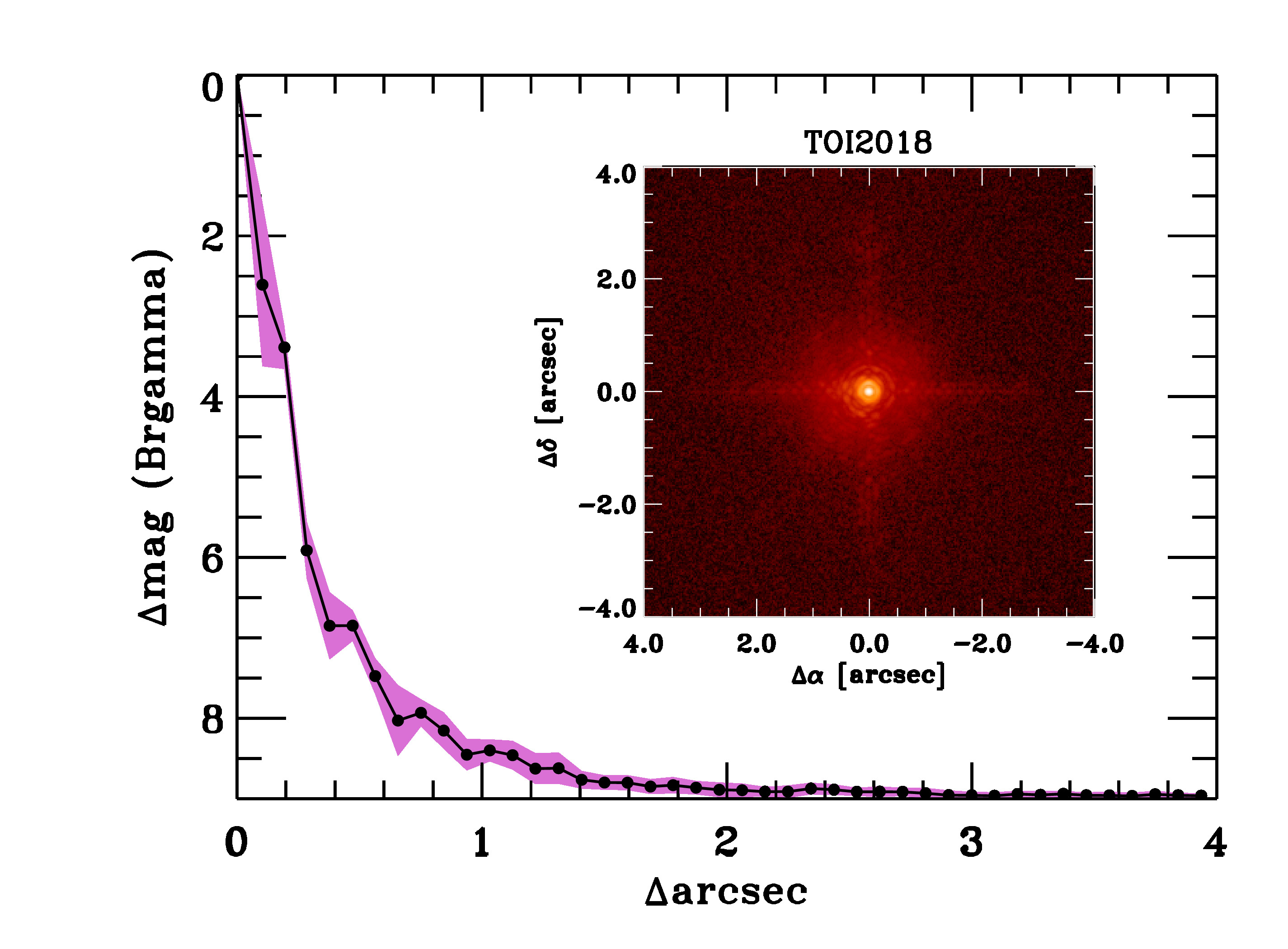
We present the Palomar/PHARO result here as an example. All other high-resolution imaging results did not detect any nearby stellar companions, and they are available on the ExoFOP website ²²2https://exofop.ipac.caltech.edu/tess/. The Palomar observations were made with the PHARO instrument (Hayward et al., 2001) behind the natural guide star AO system P3K (Dekany et al., 2013) on 2021 Jun 19 UT in a standard 5-point quincunx dither pattern with steps of 5″ in the narrow-band $Br-\gamma$ filter $(\lambda_{o}=2.1686;\Delta\lambda=0.0326~{}\mu$ m). Each dither position was observed three times, offset in position from each other by 0.5″ for a total of 15 frames; with an integration time of 1.4 seconds per frame, the total on-source time was 14 seconds. PHARO has a pixel scale of $0.025\arcsec$ per pixel for a total field of view of $\sim 25\arcsec$ . The science frames were flat-fielded and sky-subtracted. The reduced science frames were combined into a single combined image with a final resolution of 0.091″FWHM.

To within the limits of the AO observations, no stellar companions were detected. The sensitivities of the final combined AO image were determined by injecting simulated sources azimuthally around the primary target every $20^{\circ}$ at separations of integer multiples of the central source’s FWHM (Furlan et al., 2017; Lund & Ciardi, 2020). The brightness of each injected source was scaled until standard aperture photometry detected it with $5\sigma$ significance. The resulting brightness of the injected sources relative to TOI-2018 set the contrast limits at that injection location. The final $5\sigma$ limit at each separation was determined from the average of all of the determined limits at that separation. The uncertainty on the limit was set by the root-mean-square dispersion of the azimuthal slices at a given radial distance (Fig. 4).

In addition to the high-resolution imaging, we also utilized Gaia to identify any wide stellar companions that may be bound members of the system. Typically, these stars are already in the TESS Input Catalog and their flux dilution to the transit has already been accounted for in the transit fits and associated derived parameters. Based upon similar parallaxes and proper motions (e.g., Mugrauer & Michel, 2020, 2021; Mugrauer et al., 2022), there are no additional widely separated companions identified by Gaia. Additionally, the Gaia DR3 astrometry provides additional information on the possibility of inner companions that may have gone undetected by either Gaia or high-resolution imaging. The Gaia Renormalised Unit Weight Error (RUWE) is a metric similar to a reduced chi-square, where values that are $\lesssim 1.4$ indicate that the Gaia astrometric solution is consistent with the star being single. In contrast, RUWE values $\gtrsim 1.4$ may indicate an astrometric excess noise, possibily caused by the presence of an unseen companion (e.g., Ziegler et al., 2020). TOI-2018 has a Gaia DR3 RUWE value of 1.23, indicating that the astrometric fits are consistent with the single-star model.

Refer to caption — Figure 1: The chromospheric activity of TOI-2018 (orange star) in comparison with other stars in the California Planet Search sample (Isaacson & Fischer, 2010). Both $S_{HK}$ and log $R_{\rm HK}^{\prime}$ are close to 50% percentile of stars with similar B-V color. Unfortunately, the star is too cool for applying previously calibrated age-activity relations (e.g. Mamajek & Hillenbrand, 2008).

3 Photometric Analysis

3.1 TESS Observations

TOI-2018 (TIC 357501308) was observed by the TESS mission (Ricker et al., 2014) in Sectors 24 and0 51. We started with the 2-min cadence light curve produced by the TESS Science Processing Operations Center (SPOC located at NASA Ames Research Center, Jenkins et al., 2016). The data was downloaded from the Mikulski Archive for Space Telescopes website³³3https://archive.stsci.edu which is available at the following doi:10.17909/t9-nmc8-f686 (catalog DOI). Our subsequent analysis was based on the Presearch Data Conditioning Simple Aperture Photometry (PDCSAP; Stumpe et al., 2012, 2014; Smith et al., 2012) version of the light curves, although the Simple Aperture Photometry (SAP, Twicken et al., 2010; Morris et al., 2020) version was used to measure the stellar rotation period since it better preserves any long-term stellar variability. We excluded anomalous data points that have non-zero Quality flags. We note that the SPOC pipeline found a difference imaging centroid offset that is only 0.945 $\pm$ 2.55”; this is again consistent with a lack of nearby stellar companion for TOI-2018.

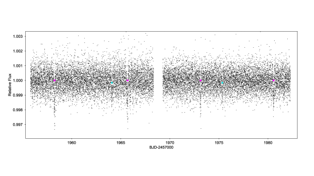
We removed any stellar activity or instrumental effects by fitting the light curve with a cubic spline in time of a width of 0.75 days. We searched for planetary transit signals in the detrended light curve using the Box-Least-Square algorithm (BLS, Kovács et al., 2002). Our pipeline has previously used for the detection of other K2 and TESS planets (Dai et al., 2017, 2021). We detected a 7.4-day planet with a signal detection efficiency (as defined by Kovács et al., 2002) of 11.7. The same candidate was reported by the TESS team (Guerrero et al., 2021) as TOI-2018.01. We also detected a second planet candidate at 11.3 day with a signal detection efficiency of 5.8 which is below the SPOC signal detection limit (SNR = 7.1). Given the low SNR of the detection, TOI-2018.02 does not meet the usual threshold for qualifying as a planet candidate. However, the orbital periods of the two planets are close to a 3:2 mean-motion resonance with a small deviation of $(P_{\rm out}/P_{\rm in})/(3/2)-1\approx 1\%$ which may boost the case for a real planet for TOI-2018.02. We did not find any other significant transit signal in the TESS light curve. Fig. 5 shows the detrended light curve and the transits of the two candidate planets.

We used the Python package Batman (Kreidberg, 2015) to model the transit light curves of the two planets simultaneously. One of the global parameters is the mean stellar density of the host $\rho=2.39\pm 0.09\rho_{\odot}$ as derived in Section 2. We imposed a Gaussian prior on the mean stellar density to help break the degeneracy in semi-major axis and impact parameter. Two other global parameters are the quadratic limb darkening coefficients using the reparameterization of $q_{1}$ and $q_{2}$ suggested by Kipping (2013). We adopted a Gaussian prior using the theoretical values from EXOFAST (Eastman et al., 2013) and a standard deviation of 0.3. Both planets were assumed to have circular orbits, hence the other transit parameters are the orbital period $P_{\text{orb}}$ , the time of conjunction $T_{\text{c}}$ , the planet-to-star radius ratio $R_{\text{p}}/R_{\star}$ , the scaled orbital distance $a/R_{\star}$ , and the transit impact parameter $b$ .

We started by assuming that both planet candidates have linear ephemerides (i.e. no transit timing variations). We fitted all transits of each planet with a constant period model. The best-fit model was determined with the Levenberg-Marquardt method implemented in Python package lmfit (Newville et al., 2014). This best-fit model was used as a template transit to fit the mid-transit times of each individual transit. During the fit of individual transits, we varied only the mid-transit time and three parameters of a quadratic function of time that describes any residual long-term variations. A total of 6 and 3 transits were observed for the two planet candidates. We were not able to detect a statistically significant transit timing variation trend for either planet. We note that the transits of TOI-2018.02 in Sector 51 were either located in data gaps or near the end of the TESS observation (Fig. 5). TOI-2018.02 could not be recovered using Sector 51 data alone. Our ephemeris of TOI-2018.02 is based on a joint fit using all sectors from TESS, the result has substantial uncertainty (Tab. 4) due to the ambiguity of the transit time in Sector 51. TESS will observe this system again in Sector 77 and 78; those data will be instrumental in confirming TOI-2018.02 and for detecting transit timing variations. We carried out a Monte Carlo Markov Chain analysis using the emcee package (Foreman-Mackey et al., 2013). We initialized 128 walkers near the best-fit model from lmfit. We ran the MCMC for 50000 links which is more than two orders of magnitude longer than the typical autocorrelation function ( $\lesssim 300$ links). The resultant posterior distribution is summarized in Table 4. Fig. 6 shows the phase folded and binned light curves for each planet candidate as well as the best-fit transit model.

3.2 MuSCAT2 Observations

We observed two egresses of TOI-2018 b with the multi-band imager MuSCAT2 (Narita et al., 2019) mounted on the 1.5 m Telescopio Carlos Sánchez (TCS) at Teide Observatory, Spain. We obtained simultaneous $g^{\prime}$ , $r^{\prime}$ , $i^{\prime}$ , and $z_{s}$ photometry on the nights of 15 June 2022 and 17 March 2023. We performed basic data reduction (dark and flat correction), aperture photometry, and transit model fit including systematics with the MuSCAT2 pipeline (Parviainen et al., 2019). On both nights, we detected the egress of TOI-2018 b; the transit did not present any significant transit depth variations across the four MuSCAT2 bands. The transit times align well with those predicted from the TESS light curve with no apparent transit timing variations. A joint fit of transit times from TESS and MuSCAT2 refined the transit ephemeris of TOI-2018 b: $P_{\rm orb}=$ 7.435569 $\pm$ 0.000081 days; $T_{c}$ (BJD-2457000) = 1958.25782 $\pm$ 0.00058. The MuSCAT2 data is available on the ExoFOP website.

3.3 WASP Observations

TOI-2018 was observed by the WASP survey (Pollacco et al., 2006) from UT May 3 2004 to Jun 28 2007. The data is available at the following link ⁴⁴4https://exoplanetarchive.ipac.caltech.edu/docs/SuperWASPMission.html. We could not recover the transit signal of either TOI-2018 b and TOI-2018.02 in the WASP light curve (non-detection is expected given WASP light curve quality). However, the much longer observational baseline of WASP provides a better constraint on the stellar rotation period than the TESS light curve.

4 Radial Velocity Analysis

We acquired a total of 38 high-resolution spectra of TOI-2018 on the Keck/HIRES (Vogt et al., 1994) from UT Jun 18 2011 to Aug 30 2021. These spectra were obtained with iodine cell in the path of light. The iodine cell served as the reference for our wavelength solution and the line spread function. The exposure time is typically 300-600 seconds after which we obtained a median SNR of 140 per reduced pixel near 5500 Å. We extracted the radial velocity using our forward-modeling Doppler code described in Howard et al. (2010). The estimated radial velocity uncertainty is about 1.2 m s^-1. The extracted radial velocities and stellar activity indices are shown in Table 5.

We assumed that the planets are on circular orbits. We also experimented with non-zero eccentricities. However, the data at hand is not sufficiently constraining. The posterior samples prefer circular models with a $\Delta$ BIC>10. We simplified our analysis by focusing on circular orbits only. With circular orbits, the radial velocity signals are hence described by the orbital period $P_{\rm orb}$ , the time of inferior conjunction $T_{c}$ , and the RV semi-amplitude $K$ . We also included an RV offset $\gamma$ , a linear RV trend $\dot{\gamma}$ , and a jitter term $\sigma_{jit}$ to account for any residual astrophysical or instrumental radial velocity uncertainties. We imposed Gaussian priors on $P_{\rm orb}$ and $T_{c}$ using the posterior distribution obtained from transit analysis. We imposed log-uniform priors on the RV semi-amplitude $K$ and the jitter $\sigma_{\text{jit}}$ . We imposed uniform priors on the RV offset $\gamma$ and linear trend $\dot{\gamma}$ . To model the influence of stellar activity contamination in the RV dataset, we employed a Gaussian Process (GP) model (e.g. Haywood et al., 2014; Grunblatt et al., 2015; Dai et al., 2017) with a quasi-periodic kernel:

\begin{split}C_{i,j}=h^{2}\exp{\left[-\frac{(t_{i}-t_{j})^{2}}{2\tau^{2}}-\Gamma\sin^{2}{\frac{\pi(t_{i}-t_{j})}{T}}\right]}\\ +\left[\sigma_{i}^{2}+\sigma_{\text{jit}}^{2}\right]\delta_{i,j}\end{split}

(1)

where $t_{i}$ is the time of individual RV measurements; $C_{i,j}$ is the covariance matrix; $\delta_{i,j}$ is the Kronecker delta function; $h$ is the amplitude of the covariance; $\tau$ is the correlation timescale; $\Gamma$ quantifies the relative significance between the squared exponential and periodic parts of the kernel; $T$ is the period of the covariance; $\sigma_{i}$ is the internal RV uncertainty and $\sigma_{jit}$ is the jitter term.

The corresponding likelihood function is:

\log{\mathcal{L}}=-\frac{N}{2}\log{2\pi}-\frac{1}{2}\log{|\bf{C}|}-\frac{1}{2}\bf{r}^{\text{T}}\bf{C}^{-\text{1}}\bf{r}

(2)

where $N$ is the total number of RV measurements; and $\bf{r}$ is the residual after subtracting the Keplerian planetary signals from the observed RV variation.

We first trained the GP model on the out-of-transit light curves first. The underlying assumption is that the stellar surface magnetic activity drives both the out-of-transit flux variation in the light curve as well as a spurious quasi-sinusoidal contamination in RV measurement. Since the out-of-transit light curve is measured to higher precision and better sampled. We conditioned all the Gaussian process hyper-parameters on the light curves first before using those hyper-parameters in the radial velocity analysis.

We experimented with including increasingly more complexity to our radial velocity models. We increased the number of planets included and if a GP model for stellar activity was warranted by the RV data set; and if a linear RV trend $\dot{\gamma}$ was required. We selected the best model by examining the Bayesian Information Criterion (BIC) after model optimization with the Levenberg-Marquardt method lmfit (Newville et al., 2014). The model favored by the current dataset contains only planet b, a long-term RV drift ( $\dot{\gamma}$ ), and a GP model for the stellar activity. We sampled the posterior distribution of this model using a similar sampling procedure as described in Section 3 using emcee. We performed two separate samplings. The posterior distribution of the various hyperparameters from an MCMC analysis of the WASP light curve was used a prior for a subsequent RV analysis. The underlying assumption is that the light curve is dominated by quasi-periodic flux variations due to the host’s stellar activity. We summarize the posterior distribution of RV analysis in Table 4. The radial velocity variation of planet b is securely detected with more than 4- $\sigma$ significance (Fig. 7). We note that the radial velocity alone was able to independently discover planet b, the ephemeris of the planet from the transit analysis was crucial for recovering the radial velocity signal. A linear RV drift $\dot{\gamma}$ is marginally detected at -0.0017 $\pm$ 0.0008 m s^-1 day^-1 over the 10-year baseline of our HIRES observation. Unfortunately, the orbital period of TOI-2018.02 is close to the first harmonic of the rotation period (11.3-day v.s. 23.5/2 days, Fig. 8). We were only able to place an upper limit on the mass of TOI-2018.02 (<3.6 $M_{\oplus}$ or $K<1.5$ m s^-1 at a 95% confidence level). Given the RV non-detection and the fact that only three transits were observed by TESS, we report TOI-2018.02 only as a possible planet candidate.

Table 4: Model Parameters of TOI-2018

Parameter	Symbol	TOI-2018 b	TOI-2018.02
From Transit Modeling
Mean Stellar Density ( $\rho_{\odot}$ )	$\rho_{\star}$	$2.29\pm 0.22$	-
Limb Darkening Coefficient	$q1$	$0.36\pm 0.22$	-
Limb Darkening Coefficient	$q2$	$0.33\pm 0.23$	-
Orbital Period (days)	$P_{\rm orb}$	$7.435583\pm 0.000022$	$11.244\pm 0.025$
Time of Conjunction (BJD-2457000)	$t_{c}$	$1958.2580\pm 0.0013$	$1964.110\pm 0.020$
Planet/Star Radius Ratio	$R_{p}/R_{\star}$	$0.0335\pm 0.0010$	$0.0228\pm 0.0020$
Impact Parameter	$b$	$0.546\pm 0.070$	$0.16\pm 0.11$
Scaled Semi-major Axis	$a/R_{\star}$	$21.12\pm 0.69$	$27.82\pm 0.90$
Transit Duration (hours)	$T_{\rm 14}$	$2.360\pm 0.090$	$3.09\pm 0.12$
Orbital Inclination (deg)	$i$	$88.52\pm 0.22$	$89.66\pm 0.31$
Orbital Eccentricity	$e$	0 (fixed)	0 (fixed)
From Radial Velocity Modeling
Semi-Amplitude (m s^-1)	$K$	$4.4\pm 1.0$	$<1.5$
Gaussian Process Amplitude (m s^-1)	$h$	$5.0\pm 1.1$	-
Gaussian Process Correlation Timescale (days)	$\tau$	$14.9^{+12.9}_{-9.4}$	-
Gaussian Process Periodicity (days)	$T$	$22.5\pm 2.1$	-
Gaussian Process Weighting	$\Gamma$	$1.5\pm 0.3$	-
RV Offset (m s^-1)	$\gamma$	$7.5\pm 3.8$	-
RV Jitter (m s^-1)	$\sigma_{\rm jit}$	$0.38^{+0.50}_{-0.24}$	-
RV Drift (m s^-1 day^-1)	$\dot{\gamma}$	$-0.0017\pm 0.0008$	-
Derived Parameters
Planetary Radius ( $R_{\oplus}$ )	$R_{\rm p}$	$2.268\pm 0.069$	$1.54\pm 0.14$
Planetary Mass ( $M_{\oplus}$ )	$M_{\rm p}$	$9.2\pm 2.1$	$<3.6$

5 Discussion

In Fig. 9, we plot the measured masses and radii of the TOI-2018 planets and other confirmed exoplanets from the NASA Exoplanet Archive⁵⁵5https://exoplanetarchive.ipac.caltech.edu. We also show various theoretical mass-radius relationships from Zeng et al. (2016) including 100%-Fe, 100%-MgSiO₃, and 100%-H₂O. In addition, we used the model by Chen & Rogers (2016) to generate the mass-radius relationships of planets with an Earth-like core and a H/He envelope of 0.5% and 1% in mass, taking into account the age and insolation of the planet as well. TOI-2018 b lies between 0.5% and 1% of H/He. However, TOI-2018 b is also consistent with an ice-rock mixture (H₂O-MgSiO₃). If we adopt a simple two-layer model (Zeng et al., 2016), TOI-2018 b is consistent with a 50%H₂O-50%MgSiO₃ composition, with a large uncertainty of about 50 $\pm$ 30% in the water mass fraction. We also showed the updated mass-radius curves for water worlds when supercritical water is included in the equation of state (Aguichine et al., 2021). TOI-2018 b is consistent with having a 20%-by-mass water/steam layer on top of an Earth-like core when the supercritical state is accounted for. With only mass and radius measurements, one can not distinguish between a H/He enveloped TOI-2018 b from a water-world TOI-2018 b. This ambiguity in composition is common to many exoplanets, which is why it has been difficult to resolve the ongoing debate over whether the observed bimodal radius distribution for sub-Neptune planets (Fulton et al., 2017) is due to the atmrospheric erosion of H/He envelopes (e.g. Owen & Wu, 2017a, b; Lopez & Fortney, 2014; Ginzburg et al., 2018) or the core growth model that gives rise to water worlds (e.g. Zeng et al., 2019; Luque & Pallé, 2022; Piaulet et al., 2023). As noted by Luque & Pallé (2022), late-type stars may be well suited to settle this debate. Water worlds are erioxpected to form beyond the snowline in the disk before migrating to the close-in orbits we see them in today. For late-type stars, the snowlines are generally much closer to the host star (Kennedy & Kenyon, 2009). Moreover, Type-I migration proceeds faster for planets with a higher planet-to-star mass ratio (see Kley & Nelson, 2012, and references therein). The short migration scale and faster Type-I migration rate both favor the migration of water worlds toward the late-type star. Disk migration might have deposited a sample of close-in water worlds (typically 50%H₂O-50%MgSiO₃) around late-type host stars as reported by Luque & Pallé (2022). The composition of TOI-2018 b is consistent with a water-world interpretation. If future follow-up observations could confirm TOI-2018.02 and its near-resonant (1% wide of 3:2) configuration with TOI-2018 b, it would further support the hypothesis that the planets underwent inward migration. This is because Type-I migration is a primary channel for capturing planets into mean-motion resonances (e.g. Kley & Nelson, 2012; Batygin, 2015; Macdonald & Dawson, 2018). Brewer et al. (2018) reported evidence that the fraction of compact, multi-planet systems is enhanced around low-metallicity host stars. If TOI-2018.02 can be confirmed by future observations, TOI-2018 presents another example of such an orbital architecture around a low-metallicity star.

With a mass of $9.2\pm 2.1M_{\oplus}$ , TOI-2018 b is close to the threshold for run-away accretion and hence giant planet formation (Rafikov, 2006; Lee & Chiang, 2015; Lee, 2019). Moreover, the low-metallicity (hence low opacity) envelope of the planet should have cooled more easily and facilitated further accretion (Lee & Chiang, 2015). Within the validity of these models, it might seem strange that TOI-2018 b failed to undergo run-away accretion given the large core mass. Could this somehow be related to the suppressed occurrence rate of gas giant planets around low-metallicity host stars (Fischer & Valenti, 2005)? One possible explanation is that the disk lifetime is much shorter around lower-metallicity stars, as suggested by Yasui et al. (2010). Theoretically, the efficiency of the photoevaporation (and dissipation) of protoplanetary disks is enhanced at lower metallicity (the timescale for disk photoevaporation $t_{\rm phot}\propto Z^{0.52}$ Ercolano & Clarke, 2010). See also more recent hydrodynamic simulations by Nakatani et al. (2018). It may be the case that TOI-2018 b did not have enough time to initiate run-away accretion before the disk dissipated. Another relevant work by Wilson et al. (2022) suggested that mini-Neptunes around low-metallicity host stars tend to have higher mean densities. It may indeed be the case that mini-Neptunes around low-metallicity stars typically does not accrete a thick envelope before the disk dissipates.

One measurement that may distinguish a planet with H/He envelope and a water world is to look for metastable Helium absorption due to the exosphere of the planet in the near infrared (e.g. Oklopčić & Hirata, 2018; Spake et al., 2018). K-type stars are ideal targets for metastable Helium observation thanks to their balance of extreme UV to far UV flux which respectively excites and destroys the metastable He population (Oklopčić, 2019; Wang & Dai, 2021). A substantial metastable He population in turn leads to the absorption of the 10830 Å transition. With a J-band magnitude of 7.8 and a moderately active K-type host, TOI-2018 b is a favorable target to look for metastable Helium absorption. The detection of ongoing Helium escape would strongly favor a H/He envelope that has survived photoevaporation.

We quantify the observability of TOI-2018 b in transmission spectroscopy using the James Webb Space Telescope (JWST, Gardner et al., 2006). We computed the Transmission Spectroscopy Metric (TSM) as suggested by Kempton et al. (2018). TOI-2018 b has a TSM of roughly 103. Although there are dozens of known exoplanets that have a higher TSM (Fig. 10), TOI-2018 b does provide a rare opportunity to probe the atmospheric composition of planets formed in a low-metallicity environment. It is one of the top-ranking TSM targets with [Fe/H]<-0.5. Given how bright the host is (J=7.8, K=7.1), special attention of the choice of instruments and observation modes is required to avoid saturation.

Previous results by Brinkman et al. (2022) and Demangeon et al. (2021) may suggest that super-Earths formed around low-metallicity late-type stars (L 98-59 M dwarf [Fe/H] = -0.46 $\pm 0.26$ and TOI-561 K dwarf [Fe/H] = -0.41 $\pm 0.05$ ) have lower mean densities than super-Earths around Sun-like stars. A similar trend was also pointed out by Adibekyan et al. (2021) and Castro-González et al. (2023). The lower mean densities may be the result of an alternative planet formation pathway in the low-metallicity regime. The enhanced $\alpha$ -element abundance (Mg, Ca, Si) compared to Fe naturally favors the formation of a larger mantle than an iron/nickel core. If so, one might expect planets around low-metallicity stars (particularly thick disk stars) to have lower mean densities compared to solar-type stars. The literature contains only a handful of mass and radius measurements for planets around low-metallicity host stars ([Fe/H] < -0.4). More metal-poor systems and more precise characterization of these planets are needed to evaluate their composition as a population.

ACKNOWLEDGEMENTS We thank Heather Knutson, Yayaati Chachan, Kento Masuda, and Yanqin Wu for helpful discussion. This material is based on work supported by the TESS General Investigator program under NASA grant 80NSSC20K0059. D.H. acknowledges support from the Alfred P. Sloan Foundation, the National Aeronautics and Space Administration (80NSSC21K0652), and the Australian Research Council (FT200100871). J.M.A.M. is supported by the National Science Foundation (NSF) Graduate Research Fellowship Program under Grant No. DGE-1842400. J.M.A.M. acknowledges the LSSTC Data Science Fellowship Program, which is funded by LSSTC, NSF Cybertraining Grant No. 1829740, the Brinson Foundation, and the Moore Foundation; his participation in the program has benefited this work. This article is based on observations made with the MuSCAT2 instrument, developed by ABC, at Telescopio Carlos Sánchez operated on the island of Tenerife by the IAC in the Spanish Observatorio del Teide. This work is partly financed by the Spanish Ministry of Economics and Competitiveness through grants PGC2018-098153-B-C31. This work is partly supported by JSPS KAKENHI Grant Number JP18H05439 and JST CREST Grant Number JPMJCR1761. This article is based on observations made with the MuSCAT2 instrument, developed by ABC, at Telescopio Carlos Sánchez operated on the island of Tenerife by the IAC in the Spanish Observatorio del Teide. DRC acknowledges partial support from NASA Grant 18-2XRP18_2-0007. AAB acknowledges the support of Ministry of Science and Higher Education of the Russian Federation under the grant 075-15-2020-780 (N13.1902.21.0039). The data presented herein were obtained at the W. M. Keck Observatory, which is operated as a scientific partnership among the California Institute of Technology, the University of California and the National Aeronautics and Space Administration. The Observatory was made possible by the generous financial support of the W. M. Keck Foundation. The authors wish to recognize and acknowledge the very significant cultural role and reverence that the summit of Maunakea has always had within the indigenous Hawaiian community. We are most fortunate to have the opportunity to conduct observations from this mountain. We acknowledge the use of public TESS data from pipelines at the TESS Science Office and at the TESS Science Processing Operations Center. Resources supporting this work were provided by the NASA High-End Computing (HEC) Program through the NASA Advanced Supercomputing (NAS) Division at Ames Research Center for the production of the SPOC data products. J. L.-B. acknowledges financial support from the Spanish Ministerio de Ciencia e Innovacion (MCINAEI 10.13039501100011033) and the European Union NextGeneration EU/PRTR under the Ramony Cajal program with code RYC2021031640I. Based on observations collected at the Centro Astronomico Hispano en Andalucia (CAHA) at Calar Alto, operated jointly by Junta de Andalucia and Consejo Superior de Investigaciones Cientificas (IAA-CSIC). A.C.-G. is funded by the Spanish Ministry of Science through MCIN/AEI/10.13039/501100011033 grant PID2019-107061GB-C61. This paper made use of data collected by the TESS mission and are publicly available from the Mikulski Archive for Space Tele- scopes (MAST) operated by the Space Telescope Science Institute (STScI). Funding for the TESS mission is provided by NASA’s Science Mission Directorate. Some of the observations in this paper made use of the High-Resolution Imaging instrument ‘Alopeke and were obtained under Gemini LLP Proposal Number: GN/S-2021A-LP-105. ‘Alopeke was funded by the NASA Exoplanet Exploration Program and built at the NASA Ames Research Center by Steve B. Howell, Nic Scott, Elliott P. Horch, and Emmett Quigley. Alopeke was mounted on the Gemini North telescope of the international Gemini Observatory, a program of NSF’s OIR Lab, which is managed by the Association of Universities for Research in Astronomy (AURA) under a cooperative agreement with the National Science Foundation. on behalf of the Gemini partnership: the National Science Foundation (United States), National Research Council (Canada), Agencia Nacional de Investigación y Desarrollo (Chile), Ministerio de Ciencia, Tecnología e Innovación (Argentina), Ministério da Ciência, Tecnologia, Inovações e Comunicações (Brazil), and Korea Astronomy and Space Science Institute (Republic of Korea).

References

Adibekyan et al. (2021) Adibekyan, V., Dorn, C., Sousa, S. G., et al. 2021, Science, 374, 330
Aguichine et al. (2021) Aguichine, A., Mousis, O., Deleuil, M., & Marcq, E. 2021, ApJ, 914, 84
Albareti et al. (2017) Albareti, F. D., Allende Prieto, C., Almeida, A., et al. 2017, ApJS, 233, 25
Arenou et al. (2018) Arenou, F., Luri, X., Babusiaux, C., et al. 2018, A&A, 616, A17
Asplund et al. (2021) Asplund, M., Amarsi, A. M., & Grevesse, N. 2021, A&A, 653, A141
Batygin (2015) Batygin, K. 2015, MNRAS, 451, 2589
Bensby et al. (2014) Bensby, T., Feltzing, S., & Oey, M. S. 2014, A&A, 562, A71
Blanco-Cuaresma (2019) Blanco-Cuaresma, S. 2019, MNRAS, 486, 2075
Blanco-Cuaresma et al. (2014) Blanco-Cuaresma, S., Soubiran, C., Heiter, U., & Jofré, P. 2014, A&A, 569, A111
Borucki et al. (2011) Borucki, W. J., Koch, D. G., Basri, G., et al. 2011, ApJ, 728, 117
Bouma et al. (2023) Bouma, L. G., Palumbo, E. K., & Hillenbrand, L. A. 2023, ApJ, 947, L3
Bouma et al. (2022) Bouma, L. G., Kerr, R., Curtis, J. L., et al. 2022, arXiv e-prints, arXiv:2205.01112
Brewer et al. (2018) Brewer, J. M., Wang, S., Fischer, D. A., & Foreman-Mackey, D. 2018, ApJ, 867, L3
Brinkman et al. (2022) Brinkman, C., Weiss, L. M., Dai, F., et al. 2022, arXiv e-prints, arXiv:2210.06665
Buder et al. (2021) Buder, S., Sharma, S., Kos, J., et al. 2021, MNRAS, 506, 150
Capitanio et al. (2017) Capitanio, L., Lallement, R., Vergely, J. L., Elyajouri, M., & Monreal-Ibero, A. 2017, A&A, 606, A65
Carrillo et al. (2020) Carrillo, A., Hawkins, K., Bowler, B. P., Cochran, W., & Vanderburg, A. 2020, MNRAS, 491, 4365
Casagrande et al. (2021) Casagrande, L., Lin, J., Rains, A. D., et al. 2021, MNRAS, 507, 2684
Castro-González et al. (2023) Castro-González, A., Demangeon, O. D. S., Lillo-Box, J., et al. 2023, arXiv e-prints, arXiv:2305.04922
Chen & Rogers (2016) Chen, H., & Rogers, L. A. 2016, ApJ, 831, 180
Choi et al. (2016a) Choi, J., Dotter, A., Conroy, C., et al. 2016a, ApJ, 823, 102
Choi et al. (2016b) —. 2016b, ApJ, 823, 102
Ciardi et al. (2015) Ciardi, D. R., Beichman, C. A., Horch, E. P., & Howell, S. B. 2015, ApJ, 805, 16
Collins et al. (2017) Collins, K. A., Kielkopf, J. F., Stassun, K. G., & Hessman, F. V. 2017, AJ, 153, 77
Cui et al. (2012) Cui, X.-Q., Zhao, Y.-H., Chu, Y.-Q., et al. 2012, Research in Astronomy and Astrophysics, 12, 1197
Dai et al. (2017) Dai, F., Winn, J. N., Gandolfi, D., et al. 2017, AJ, 154, 226
Dai et al. (2021) Dai, F., Howard, A. W., Batalha, N. M., et al. 2021, AJ, 162, 62
Dekany et al. (2013) Dekany, R., Roberts, J., Burruss, R., et al. 2013, ApJ, 776, 130
Demangeon et al. (2021) Demangeon, O. D. S., Zapatero Osorio, M. R., Alibert, Y., et al. 2021, A&A, 653, A41
Eastman et al. (2013) Eastman, J., Gaudi, B. S., & Agol, E. 2013, PASP, 125, 83
Ercolano & Clarke (2010) Ercolano, B., & Clarke, C. J. 2010, MNRAS, 402, 2735
Evans et al. (2018) Evans, D. W., Riello, M., De Angeli, F., et al. 2018, A&A, 616, A4
Fabricius et al. (2021) Fabricius, C., Luri, X., Arenou, F., et al. 2021, A&A, 649, A5
Feroz et al. (2009) Feroz, F., Hobson, M. P., & Bridges, M. 2009, MNRAS, 398, 1601
Feroz et al. (2013) Feroz, F., Hobson, M. P., Cameron, E., & Pettitt, A. N. 2013, ArXiv e-prints, arXiv:1306.2144
Fischer & Valenti (2005) Fischer, D. A., & Valenti, J. 2005, ApJ, 622, 1102
Foreman-Mackey et al. (2013) Foreman-Mackey, D., Hogg, D. W., Lang, D., & Goodman, J. 2013, PASP, 125, 306
Fressin et al. (2013) Fressin, F., Torres, G., Charbonneau, D., et al. 2013, ApJ, 766, 81
Fulton et al. (2017) Fulton, B. J., Petigura, E. A., Howard, A. W., et al. 2017, AJ, 154, 109
Furlan et al. (2017) Furlan, E., Ciardi, D. R., Everett, M. E., et al. 2017, AJ, 153, 71
Gagné et al. (2018) Gagné, J., Mamajek, E. E., Malo, L., et al. 2018, ApJ, 856, 23
Gaia Collaboration et al. (2016) Gaia Collaboration, Prusti, T., de Bruijne, J. H. J., et al. 2016, A&A, 595, A1
Gaia Collaboration et al. (2018) Gaia Collaboration, Brown, A. G. A., Vallenari, A., et al. 2018, A&A, 616, A1
Gaia Collaboration et al. (2022) Gaia Collaboration, Vallenari, A., Brown, A. G. A., et al. 2022, arXiv e-prints, arXiv:2208.00211
Gardner et al. (2006) Gardner, J. P., Mather, J. C., Clampin, M., et al. 2006, Space Sci. Rev., 123, 485
Gavel et al. (2014) Gavel, D., Kupke, R., Dillon, D., et al. 2014, in Society of Photo-Optical Instrumentation Engineers (SPIE) Conference Series, Vol. 9148, Adaptive Optics Systems IV, ed. E. Marchetti, L. M. Close, & J.-P. Vran, 914805
Ginzburg et al. (2018) Ginzburg, S., Schlichting, H. E., & Sari, R. 2018, MNRAS, 476, 759
Gonzalez (1997) Gonzalez, G. 1997, MNRAS, 285, 403
Grunblatt et al. (2015) Grunblatt, S. K., Howard, A. W., & Haywood, R. D. 2015, ApJ, 808, 127
Guerrero et al. (2021) Guerrero, N. M., Seager, S., Huang, C. X., et al. 2021, ApJS, 254, 39
Gustafsson et al. (2008) Gustafsson, B., Edvardsson, B., Eriksson, K., et al. 2008, A&A, 486, 951
Hambly et al. (2018) Hambly, N. C., Cropper, M., Boudreault, S., et al. 2018, A&A, 616, A15
Hayashi (1981) Hayashi, C. 1981, Progress of Theoretical Physics Supplement, 70, 35
Hayward et al. (2001) Hayward, T. L., Brandl, B., Pirger, B., et al. 2001, PASP, 113, 105
Haywood et al. (2014) Haywood, R. D., Collier Cameron, A., Queloz, D., et al. 2014, MNRAS, 443, 2517
Hormuth et al. (2008) Hormuth, F., Brandner, W., Hippler, S., & Henning, T. 2008, Journal of Physics Conference Series, 131, 012051
Howard et al. (2010) Howard, A. W., Johnson, J. A., Marcy, G. W., et al. 2010, ApJ, 721, 1467
Howard et al. (2012) Howard, A. W., Marcy, G. W., Bryson, S. T., et al. 2012, ApJS, 201, 15
Howell et al. (2011) Howell, S. B., Everett, M. E., Sherry, W., Horch, E., & Ciardi, D. R. 2011, AJ, 142, 19
Huber et al. (2017) Huber, D., Zinn, J., Bojsen-Hansen, M., et al. 2017, ApJ, 844, 102
Isaacson & Fischer (2010) Isaacson, H., & Fischer, D. 2010, ApJ, 725, 875
Jenkins et al. (2016) Jenkins, J. M., Twicken, J. D., McCauliff, S., et al. 2016, in Proc. SPIE, Vol. 9913, Software and Cyberinfrastructure for Astronomy IV, 99133E
Kempton et al. (2018) Kempton, E. M. R., Bean, J. L., Louie, D. R., et al. 2018, PASP, 130, 114401
Kennedy & Kenyon (2009) Kennedy, G. M., & Kenyon, S. J. 2009, ApJ, 695, 1210
Kipping (2013) Kipping, D. M. 2013, MNRAS, 435, 2152
Kley & Nelson (2012) Kley, W., & Nelson, R. P. 2012, ARA&A, 50, 211
Kovács et al. (2002) Kovács, G., Zucker, S., & Mazeh, T. 2002, A&A, 391, 369
Kreidberg (2015) Kreidberg, L. 2015, PASP, 127, 1161
Kupke et al. (2012) Kupke, R., Gavel, D., Roskosi, C., et al. 2012, in Society of Photo-Optical Instrumentation Engineers (SPIE) Conference Series, Vol. 8447, Adaptive Optics Systems III, ed. B. L. Ellerbroek, E. Marchetti, & J.-P. Véran, 84473G
Kurucz (1979) Kurucz, R. L. 1979, ApJS, 40, 1
Lallement et al. (2014) Lallement, R., Vergely, J. L., Valette, B., et al. 2014, A&A, 561, A91
Lallement et al. (2018) Lallement, R., Capitanio, L., Ruiz-Dern, L., et al. 2018, A&A, 616, A132
Lee (2019) Lee, E. J. 2019, ApJ, 878, 36
Lee & Chiang (2015) Lee, E. J., & Chiang, E. 2015, ApJ, 811, 41
Lee & Chiang (2016) —. 2016, ApJ, 817, 90
Lee et al. (2018) Lee, E. J., Chiang, E., & Ferguson, J. W. 2018, MNRAS, 476, 2199
Lindegren et al. (2021a) Lindegren, L., Bastian, U., Biermann, M., et al. 2021a, A&A, 649, A4
Lindegren et al. (2021b) Lindegren, L., Klioner, S. A., Hernández, J., et al. 2021b, A&A, 649, A2
Lomb (1976) Lomb, N. R. 1976, Astrophysics and Space Science, 39, 447. http://dx.doi.org/10.1007/BF00648343
Lopez & Fortney (2014) Lopez, E. D., & Fortney, J. J. 2014, ApJ, 792, 1
Lund & Ciardi (2020) Lund, M. B., & Ciardi, D. 2020, in American Astronomical Society Meeting Abstracts, Vol. 235, American Astronomical Society Meeting Abstracts #235, 249.06
Luque & Pallé (2022) Luque, R., & Pallé, E. 2022, Science, 377, 1211
Macdonald & Dawson (2018) Macdonald, M. G., & Dawson, R. I. 2018
Mamajek & Hillenbrand (2008) Mamajek, E. E., & Hillenbrand, L. A. 2008, ApJ, 687, 1264
Martig et al. (2015) Martig, M., Rix, H.-W., Silva Aguirre, V., et al. 2015, MNRAS, 451, 2230
McGurk et al. (2014) McGurk, R., Rockosi, C., Gavel, D., et al. 2014, in Society of Photo-Optical Instrumentation Engineers (SPIE) Conference Series, Vol. 9148, Adaptive Optics Systems IV, ed. E. Marchetti, L. M. Close, & J.-P. Vran, 91483A
McQuillan et al. (2014) McQuillan, A., Mazeh, T., & Aigrain, S. 2014, ApJS, 211, 24
Meléndez et al. (2014) Meléndez, J., Schirbel, L., Monroe, T. R., et al. 2014, A&A, 567, L3
Morris et al. (2020) Morris, R. L., Twicken, J. D., Smith, J. C., et al. 2020, Kepler Data Processing Handbook: Photometric Analysis, Kepler Science Document KSCI-19081-003, id. 6. Edited by Jon M. Jenkins., ,
Morton (2015) Morton, T. D. 2015, isochrones: Stellar model grid package, Astrophysics Source Code Library, record ascl:1503.010, , , ascl:1503.010
Mugrauer & Michel (2020) Mugrauer, M., & Michel, K.-U. 2020, Astronomische Nachrichten, 341, 996
Mugrauer & Michel (2021) —. 2021, Astronomische Nachrichten, 342, 840
Mugrauer et al. (2022) Mugrauer, M., Zander, J., & Michel, K.-U. 2022, Astronomische Nachrichten, 343, e24017
Nakatani et al. (2018) Nakatani, R., Hosokawa, T., Yoshida, N., Nomura, H., & Kuiper, R. 2018, ApJ, 857, 57
Narita et al. (2019) Narita, N., Fukui, A., Kusakabe, N., et al. 2019, Journal of Astronomical Telescopes, Instruments, and Systems, 5, 015001
Newville et al. (2014) Newville, M., Stensitzki, T., Allen, D. B., & Ingargiola, A. 2014, LMFIT: Non-Linear Least-Square Minimization and Curve-Fitting for Python, v0.8.0, Zenodo, doi:10.5281/zenodo.11813. https://doi.org/10.5281/zenodo.11813
Oklopčić (2019) Oklopčić, A. 2019, ApJ, 881, 133
Oklopčić & Hirata (2018) Oklopčić, A., & Hirata, C. M. 2018, ApJ, 855, L11
Owen & Wu (2017a) Owen, J. E., & Wu, Y. 2017a, ApJ, 847, 29
Owen & Wu (2017b) —. 2017b, ApJ, 847, 29
Parviainen et al. (2019) Parviainen, H., Tingley, B., Deeg, H. J., et al. 2019, A&A, 630, A89
Paxton et al. (2011) Paxton, B., Bildsten, L., Dotter, A., et al. 2011, ApJS, 192, 3
Paxton et al. (2013) Paxton, B., Cantiello, M., Arras, P., et al. 2013, ApJS, 208, 4
Paxton et al. (2015) Paxton, B., Marchant, P., Schwab, J., et al. 2015, ApJS, 220, 15
Petigura (2015) Petigura, E. A. 2015, PhD thesis, University of California, Berkeley
Petigura et al. (2013) Petigura, E. A., Howard, A. W., & Marcy, G. W. 2013, Proceedings of the National Academy of Science, 110, 19273
Petigura et al. (2018) Petigura, E. A., Marcy, G. W., Winn, J. N., et al. 2018, AJ, 155, 89
Piaulet et al. (2023) Piaulet, C., Benneke, B., Almenara, J. M., et al. 2023, Nature Astronomy, 7, 206
Pollacco et al. (2006) Pollacco, D. L., Skillen, I., Collier Cameron, A., et al. 2006, PASP, 118, 1407
Pollack et al. (1996) Pollack, J. B., Hubickyj, O., Bodenheimer, P., et al. 1996, Icarus, 124, 62 . http://www.sciencedirect.com/science/article/pii/S0019103596901906
Rafikov (2006) Rafikov, R. R. 2006, ApJ, 648, 666
Reggiani et al. (2022) Reggiani, H., Schlaufman, K. C., Healy, B. F., Lothringer, J. D., & Sing, D. K. 2022, arXiv e-prints, arXiv:2201.08508
Ricker et al. (2014) Ricker, G. R., Winn, J. N., Vanderspek, R., et al. 2014, Society of Photo-Optical Instrumentation Engineers (SPIE) Conference Series, Vol. 9143, Transiting Exoplanet Survey Satellite (TESS), 914320
Riello et al. (2018) Riello, M., De Angeli, F., Evans, D. W., et al. 2018, A&A, 616, A3
Rogers (2015) Rogers, L. A. 2015, ApJ, 801, 41
Safonov et al. (2017) Safonov, B. S., Lysenko, P. A., & Dodin, A. V. 2017, Astronomy Letters, 43, 344
Santos et al. (2004) Santos, N. C., Israelian, G., & Mayor, M. 2004, A&A, 415, 1153
Scargle (1982) Scargle, J. D. 1982, ApJ, 263, 835
Smith et al. (2012) Smith, J. C., Stumpe, M. C., Van Cleve, J. E., et al. 2012, PASP, 124, 1000
Sneden (1973) Sneden, C. 1973, ApJ, 184, 839
Sneden et al. (2012) Sneden, C., Bean, J., Ivans, I., Lucatello, S., & Sobeck, J. 2012, MOOG: LTE line analysis and spectrum synthesis, Astrophysics Source Code Library, record ascl:1202.009, , , ascl:1202.009
Spake et al. (2018) Spake, J. J., Sing, D. K., Evans, T. M., et al. 2018, Nature, 557, 68
Stassun & Torres (2016) Stassun, K. G., & Torres, G. 2016, AJ, 152, 180
Stassun et al. (2019) Stassun, K. G., Oelkers, R. J., Paegert, M., et al. 2019, AJ, 158, 138
Steinmetz et al. (2020) Steinmetz, M., Matijevič, G., Enke, H., et al. 2020, AJ, 160, 82
Stumpe et al. (2014) Stumpe, M. C., Smith, J. C., Catanzarite, J. H., et al. 2014, PASP, 126, 100
Stumpe et al. (2012) Stumpe, M. C., Smith, J. C., Van Cleve, J. E., et al. 2012, PASP, 124, 985
Tayar et al. (2022) Tayar, J., Claytor, Z. R., Huber, D., & van Saders, J. 2022, ApJ, 927, 31
Torra et al. (2021) Torra, F., Castañeda, J., Fabricius, C., et al. 2021, A&A, 649, A10
Twicken et al. (2010) Twicken, J. D., Clarke, B. D., Bryson, S. T., et al. 2010, in Society of Photo-Optical Instrumentation Engineers (SPIE) Conference Series, Vol. 7740, Software and Cyberinfrastructure for Astronomy, ed. N. M. Radziwill & A. Bridger, 774023
Vogt et al. (1994) Vogt, S. S., Allen, S. L., Bigelow, B. C., et al. 1994, in Society of Photo-Optical Instrumentation Engineers (SPIE) Conference Series, Vol. 2198, Instrumentation in Astronomy VIII, ed. D. L. Crawford & E. R. Craine, 362
Wang & Fischer (2015) Wang, J., & Fischer, D. A. 2015, AJ, 149, 14
Wang & Dai (2021) Wang, L., & Dai, F. 2021, ApJ, 914, 98
Wilson et al. (2022) Wilson, T. G., Goffo, E., Alibert, Y., et al. 2022, MNRAS, 511, 1043
Yana Galarza et al. (2019) Yana Galarza, J., Meléndez, J., Lorenzo-Oliveira, D., et al. 2019, MNRAS, 490, L86
Yasui et al. (2010) Yasui, C., Kobayashi, N., Tokunaga, A. T., Saito, M., & Tokoku, C. 2010, ApJ, 723, L113
Zeng et al. (2016) Zeng, L., Sasselov, D. D., & Jacobsen, S. B. 2016, ApJ, 819, 127
Zeng et al. (2019) Zeng, L., Jacobsen, S. B., Sasselov, D. D., et al. 2019, Proceedings of the National Academy of Sciences, 116, 9723. https://www.pnas.org/content/116/20/9723
Ziegler et al. (2020) Ziegler, C., Tokovinin, A., Briceño, C., et al. 2020, AJ, 159, 19

Table 5: Keck/HIRES Radial Velocities

Time (BJD)	RV (m/s)	RV Unc. (m/s)	$S_{HK}$	$S_{HK}$ Unc.
2455730.958602	6.07	1.45	0.862	0.001
2455734.825559	8.22	1.28	0.924	0.001
2455738.787684	4.87	1.24	0.942	0.001
2459038.821696	13.18	1.17	0.980	0.001
2459040.797956	1.46	1.28	0.943	0.001
2459041.824545	-2.66	1.16	0.976	0.001
2459057.899283	1.45	1.48	0.923	0.001
2459379.877596	10.84	1.29	0.955	0.001
2459381.996691	-1.29	1.35	0.939	0.001
2459383.007785	-3.82	1.48	0.908	0.001
2459383.838423	-8.58	1.22	0.930	0.001
2459384.840558	-11.87	1.27	0.966	0.001
2459385.899575	-10.13	1.30	0.909	0.001
2459386.771843	-5.64	1.17	0.940	0.001
2459388.873567	-5.48	1.33	0.920	0.001
2459389.835862	-4.30	1.42	0.905	0.001
2459395.8831	1.87	1.23	0.895	0.001
2459397.962232	-0.29	1.49	0.873	0.001
2459399.786738	-2.54	1.24	0.902	0.001
2459404.959869	4.76	1.14	0.922	0.001
2459405.967385	-2.93	1.26	0.949	0.001
2459406.835315	-1.98	1.15	0.935	0.001
2459408.949042	1.34	1.18	0.907	0.001
2459409.954172	3.36	1.14	0.873	0.001
2459411.773495	-0.61	1.41	0.876	0.001
2459412.953324	-2.68	1.32	0.874	0.001
2459414.954138	1.18	1.44	0.888	0.001
2459422.908053	3.78	1.51	0.889	0.001
2459435.803746	-3.35	1.23	0.854	0.001
2459443.768482	-4.01	1.16	0.857	0.001
2459444.854338	-4.55	1.14	0.875	0.001
2459446.857033	13.66	1.54	0.928	0.001
2459448.79132	11.51	1.18	0.916	0.001
2459449.79849	6.07	1.23	0.925	0.001
2459451.81223	-3.59	1.11	0.960	0.001
2459452.74112	-1.93	1.11	0.945	0.001
2459455.773054	-3.80	1.26	0.886	0.001
2459456.806188	-3.19	1.27	0.890	0.001