Systems, variational principles and interconnections in nonequilibrium thermodynamics

Abstract

The paper investigates a systematic approach to modeling in nonequilibrium thermodynamics by focusing upon the notion of interconnections, where we propose a novel Lagrangian variational formulation of such interconnected systems by extending the variational principle of Hamilton in mechanics. In particular, we show how a nonequilibrium thermodynamic system can be regarded as an interconnected system of primitive physical elements or subsystems throughout an interconnection. While this approach is new in nonequilibrium thermodynamics, this idea has been known as a useful tool for the modeling of complicated systems in networks as well as in mechanics. Hence, the setting developed in this paper yields a promising direction for building a unifying description in various areas of modern science via thermodynamic principles, while being at the same time related to the early developments of variational mechanics.

1 Introduction

1.1 Variational principle in thermodynamics

One of the most fundamental principle in physics is the Principle of Critical Action. Maxwell’s equations in electromagnetism, Newton’s equations of motion in classical mechanics, Shrödinger’s equations in quantum mechanics, Einstein’s equations in general relativity, can all be obtained by extremizing a quantity, called action functional, encoding all the properties of the system. For classical mechanics, this principle reduces to Hamilton’s principle, which enables us to systematically formulate the dynamics of conservative systems, [22]. For the cases in which a mechanical system involves a nonconservative external force and kinematic constraints, whether they are holonomic or not, the variational principle of Hamilton is replaced by the Lagrange-d’Alembert Principle, where the additional term associated to the external force must be included and in which the variations of the curves are subject to the so-called variational constraints. Regarding nonequilibrium thermodynamics, on the other hand, which includes mechanics and is also deeply related to various disciplines such as computational fluid dynamics, chemical reactions, biological and engineering systems,[4, 20], there has been a large gap with mechanics from the viewpoint of the proposed variational formulations. In other words, a variational formulation for nonequilibrium thermodynamics that includes the Hamilton action principle in mechanics as a special case has not been completely established. In fact, although there have been proposed many variational approaches such as the minimum dissipation principle by [25, 24, 23] and the minimum entropy production principle by [30, 14], these principles mainly treat the entropy production and the related dissipative energy of the thermodynamic system, while one does not know how to recover Hamilton’s principle in mechanics from these approaches when the irreversible processes are absent. In particular, it has not been clarified how to link Hamilton’s variational principle in mechanics with those variational approaches in thermodynamics. Another relevant work was done by [1, 2], in which a generalized form of d’Alembert principle called a principle of virtual dissipation was illustrated with applications to irreversible thermodynamic systems with viscoelasticity, thermoelasticity as well as heat transfer. However, it was limited to weakly irreversible systems, isothermal systems or quasi-isothermal systems, where the required constraints associated with the rate of entropy production were simplified to be holonomic or quasi-holonomic. There exists some other variational formulation in thermodynamics including mesoscopic views, including Boltzman kinetic equations, see [17]. However, it is not an extension of the variational principle of Hamilton in Lagrangian mechanics. Due to the strong connection of nonequilibrium thermodynamics with various disciplines, the understanding of this field from a variational formulation closely related to that of mechanics would also foster the identification of common principles between different disciplines and provide a promising tool for the modelling of multiphysical systems. The questions emerging from the above comments can be summarized as follows:

• What is the variational principle for nonequilibrium thermodynamics, consistent with Hamilton’s principle in mechanics?

• How can we systematically understand interconnection in the realm of nonequilibrium thermodynamic systems via variational principles?

To answer these questions, we will first show how the entropy production associated to irreversible processes can be understood as a phenomenological constraint that is nonlinear nonholonomic and also how it is incorporated into a variational principle of the Lagrange-d’Alembert type, see [9, 10, 13]. Second, with the help of network theory[21, 26, 27], we will introduce the notion of interconnections in order to represent the structure of nonequilibrium thermodynamic systems, by which one can reticulate the original system into an interconnected system of primitive systems or constituent elements throughout the energy flow. Mathematically the interconnection is represented by a Dirac structure, which is an extended notion of symplectic and Poisson structures, and provides us with an implicit relation between dual variables, namely, velocity (vector) and force (covector). It has been clarified that the constraints due to Kirchhoff Current Law and Kirchhoff Voltage Law in electric circuit and those due to nonholonomic constraints can be modeled by such interconnections, see [34]. However, it has not been systematically understood how such interconnections appear in thermodynamics. In this paper, we propose a novel idea of how the interconnection can incorporate the nonlinear phenomenological relations linked to the entropy production. It is then showed that the variational formulation of a nonequilibrium thermodynamic system can be systematically constructed by the interconnection of the variational formulation of each primitive system.

The approach that we develop in this paper is relevant for the modelling and analysis of complex systems. On one hand, the analysis of the interconnection helps recognizing the primitive entities, denoted $\boldsymbol{\Sigma}_{k}$, $k=1,...,P$, which can be of different nature (mechanical, thermal, electrical), and whose dynamics is easier to design and understand than the original system $\boldsymbol{\Sigma}=\cup_{k=1}^{P}\boldsymbol{\Sigma}_{k}$. On the other hand it allows to correctly describe the known and unknown energetic fluxes among such primitive entities $\boldsymbol{\Sigma}_{k}$ and $\boldsymbol{\Sigma}_{\ell}$, which must be consistent with the fundamental laws of thermodynamics. It has been argued that such an interconnection approach may be potentially useful beyond the setting of physical science by inspiring modeling techniques for social sciences, such as the dynamics of human society evolution, where the concepts of energy, power, and fluxes may be given some interpretations, see [29] and references therein. The development of a variational formulation for primitive systems in thermodynamics and the systematic understanding of the interconnection of such variational formulations to achieve a description of the full system thus provides a promising tool for building a common description in various areas of modern science. At the same time, such variational formulations have their roots in the critical action principle of Hamilton, and are thus connected to the early developments of classical mechanics.

The variational description also naturally yields the associated geometric structures underlying the dynamics of each subsystems as well as the interconnections of such subsystems. While we shall not consider this aspect in this paper, let us mention that a special class of Dirac structures that is induced from the interconnection constraints, called an interaction Dirac structure, behaves well in interconnecting subsystems in the sense that the variational structures associated to each subsystem are to be intertwined through the interaction Dirac structures $D_{\rm int}$ associated to the interconnection conditions. This naturally produces a variational formulation of the interconnected system which yield the equations of motion for the overall system.

2 System theoretic approach to thermodynamics

2.1 Nonequilibrium thermodynamic systems

Let us consider a thermodynamic system $\boldsymbol{\Sigma}$ which has energetic interactions with its exterior $\boldsymbol{\Sigma}^{\rm ext}$, as shown in Figure 1. The state of the thermodynamic system is described by a set of mechanical state variables $(\mathbf{q},\mathbf{v})$ and thermodynamic variables $\zeta$. Functions of these variables are referred to as state functions. Let us call $\boldsymbol{\Sigma}$ a simple system if the thermodynamic state is described in terms of a single variable $\zeta$, usually, chosen by an entropy $S$ as will be shown. Let $P^{\rm ext}_{M}(t)$ be the power exchange with exterior which is associated to the matter transfer, $P^{\rm ext}_{H}(t)$ that associated to the heat transfer, and $P^{\rm ext}_{M}(t)$ that associated to the mechanical force.

Any thermodynamic system can be classified into the following cases:

• $\boldsymbol{\Sigma}$ is closed if $P^{\rm ext}_{M}(t)=0$.

• $\boldsymbol{\Sigma}$ is adiabatically closed if $P^{\rm ext}_{M}(t)=P^{\rm ext}_{H}(t)=0$.

• $\boldsymbol{\Sigma}$ is isolated if $P^{\rm ext}_{M}(t)=P^{\rm ext}_{H}(t)=P^{\rm ext}_{W}(t)=0$.

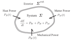
Figure 1: System with energetic interactions

2.2 Laws of nonequilibrium thermodynamics

First law.

Following [31], the first law states that for every system $\boldsymbol{\Sigma}$, there exists an extensive state function $E$, which satisfies the following relation

$$\frac{d}{dt}E(t)=P^{\rm ext}_{W}(t)+P^{\rm ext}_{H}(t)+P^{\rm ext}_{M}(t),$$ (1)

where $t$ denotes time. This function is called the energy of the system. In the case of an isolated system, the energy is conserved.

Second law.

For every system $\boldsymbol{\Sigma}$ there exists an extensive state function $S$, which satisfies the following relations

• If $\boldsymbol{\Sigma}$ is adiabatically closed, $S$ is a non-deceasing function with respect to $t$, i.e.,

  $$\frac{d}{dt}S(t)=I(t)\geq 0,$$

  where $I(t)$ is the internal entropy production rate linked to the irreversible processes.

• If $\boldsymbol{\Sigma}$ is isolated, $S$ tends to a finite local maximum as $t$ goes to infinity, namely,

  $$\lim_{t\rightarrow+\infty}S(t)=\max_{\rho\;\text{compatible}}S[\rho],$$

  where “$\rho$ compatible” indicates a thermodynamic state that is compatible with the constraints, such as isolation conditions and internal walls.

This function is called the entropy of the system.

For the case in which $\boldsymbol{\Sigma}$ is isolated, it is said to be reversible if $I(t)=0$, i.e., $S$ is constant. For the case in which the system is not isolated, it is said to be reversible if the total isolated system (formed by the system and the surrounding with which it interacts) is reversible.

2.3 Systems and interconnection

By definition, a system is a set of objects with relationships between the objects and between their attributes, see [18, 28]. In any physical system, the relationships are given in terms of power flow, i.e., throughout the energy balance, and we can interpret the objects as constituent elements of the system such as mass, spring and friction for mechanical systems, or inductors, capacitors and resistors in electric circuits, etc. Their attributes may be interpreted by the constitutive relations of physical components. The structural relations between the objects, namely, elements or subsystems, can be modeled as an interconnection, whose relationships are given by input-output relation between dual variables $\mathbf{v}$ and $\mathbf{f}$, such as velocity and force variables in mechanics, current and voltage variables in circuits, or entropy flow and temperature in thermodynamics. The associated power flow $P$ given by the dual paring as $P=\left<\mathbf{f},\mathbf{v}\right>$ vanishes, which describes the power invariance or energy balance. An instance of this relation is Tellegen’s theorem in circuit theory, see [5].

Such structural relations can be mathematically understood by symplectic, Poisson or Dirac structures on the state space $M$ and they are given among a vector field (velocity field) $X$ and a one-form (force field) $\alpha$ on $M$, where $M$ is usually the phase space, or the cotangent bundle over a configuration manifold. For instance, for a symplectic structure $\Omega:TM\times TM\to\mathbb{R}$, the structural relation is given by $\alpha=\Omega^{\flat}X$ where $\Omega^{\flat}:TM\to T^{\ast}M$ is given by $\langle\Omega^{\flat}(z)(X_{z}),Y_{z}\rangle=\Omega(z)(X_{z},Y_{z})$, $z\in M$, $X_{z},Y_{z}\in T_{z}M$. For a Poisson structure $B:T^{*}M\times T^{*}M\to\mathbb{R}$, the structural relation is given by $X=B^{\sharp}\alpha$, where the associated bundle map $B^{\sharp}:T^{\ast}M\to TM$ is defined by $B(z)(\alpha_{z},\beta_{z})=\langle\alpha_{z},B^{\sharp}(\beta_{z})\rangle$, $z\in M$, $\alpha_{z},\beta_{z}\in T^{*}_{z}M$. Finally, for a Dirac structure $D\subset TM\oplus T^{\ast}M$, the structural relations are implicitly given as $(X,\alpha)\in D$. In particular, such a structure is called an interconnection among elements or subsystems, each of which is called a primitive system; see [21, 34, 19]. In Hamiltonian mechanics, for example, the force field $\alpha$ is usually given by the differential of a given Hamiltonian function $H$ on $M$ and hence the dynamics is given in the context of symplectic structures as $\mathbf{d}H(z)=\Omega^{\flat}(z)\cdot X_{H}(z)$ for each $z\in M$, while it is given as $X_{H}(z)=B^{\sharp}(z)\mathbf{d}H(z)$ in the framework of Poisson structures. Notice that $B^{\sharp}=(\Omega^{\flat})^{-1}$ on a symplectic manifold $M$, which implies that the input and output relations are given explicitly between the force field $\mathbf{d}H$ and the velocity field $X_{H}$ but they are given in converse for symplectic and Poisson structures. For those cases, the Dirac structure may be given by $D=\mathrm{graph}\,\Omega^{\flat}$ or $D=\mathrm{graph}\,B^{\sharp}$, where the input and output relations are implicitly given between $\mathbf{d}H$ and $X_{H}$. On symplectic manifolds, by using the canonical coordinates $q^{i},p_{i},\,i=1,...,n$ for $M$, which is ensured by Darboux’s theorem, we can recover the usual Hamilton equations as $\dot{q}^{i}=\frac{\partial H}{\partial p_{i}}$ and $\dot{p}_{i}=-\frac{\partial H}{\partial{q}^{i}}$.

Example.

As an illustration, consider the thermodynamics of an electric circuit which consists of an inductor L, a capacitor C, a resistor R and a source of voltage V, as shown on Figure 2. We include the internal entropy production regarding the irreversibility of the resistor. The configuration space is $Q\times\mathbb{R}=\mathbb{R}^{5}$ which contains the charges $\mathbf{q}=(q^{1},q^{2},q^{3},q^{4})=(q_{V},q_{L},q_{R},q_{C})\in Q=\mathbb{R}^{4}$ as well as the entropy $S\in\mathbb{R}$.

The circuit can be understood as an interconnected system throughout the interconnection $\Delta_{Q}\times\Delta_{Q}^{\circ}\subset TQ\oplus T^{\ast}Q$, where the distribution $\Delta_{Q}\subset TQ$ describes the Kirchhoff circuit law (KCL) constraints among currents $\mathbf{\dot{q}}=(\dot{q}^{1},\dot{q}^{2},\dot{q}^{3},\dot{q}^{4})=(\dot{q}_{V},\dot{q}_{L},\dot{q}_{R},\dot{q}_{C})\in T_{\mathbf{q}}Q$, and where its annihilator $\Delta_{Q}^{\circ}$ defined by $\Delta_{Q}^{\circ}(\mathbf{q}):=\{\mathbf{f}\in T^{*}_{\mathbf{q}}Q\mid\left<\mathbf{f},\mathbf{\dot{q}}\right>=0,\;\;\forall\,\mathbf{\dot{q}}\in\Delta_{Q}(\mathbf{q})\}$ describes the Kirchhoff voltage law (KVL) constraints among voltages $\mathbf{f}=(f_{1},f_{2},f_{3},f_{4})=(f_{V},f_{L},f_{R},f_{C})\in T_{\mathbf{q}}^{\ast}Q$. For the present case, see Figure 2, one has

$$\Delta_{Q}(\mathbf{q})=\{\mathbf{\dot{q}}\in T_{\mathbf{q}}Q\mid\langle\omega^{a},\mathbf{\dot{q}}\rangle=0,a=1,2\},$$ (2)

with $\omega^{a}=\omega_{k}^{a}\,dq^{k},\;a=1,2;\;k=1,...,4,$ the two independent covectors given in matrix representation by

$$\omega_{k}^{a}=\left(\begin{array}[]{cccc}-1&-1&0&0\\ 0&1&-1&-1\\ \end{array}\right).$$

The interconnection $D=\Delta_{Q}\times\Delta_{Q}^{\circ}\subset TQ\oplus T^{\ast}Q$ is an example of an interaction Dirac structure, see [19].

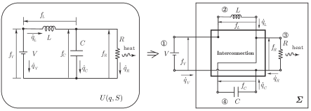
Figure 2: Interconnection of an L-C-R circuit

Furthermore, there exists an internal entropy production associated to the irreversibility of the resistor, i.e.,

$$I=\dot{S}=-\frac{1}{T}V_{R}(\mathbf{q},\dot{\mathbf{q}},S)\cdot\dot{\mathbf{q}},$$

where $\dot{(\;)}$ indicates the derivative with respect to time, $T$ is the temperature determined from the internal energy $U=U(\mathbf{q},S)$ of $\boldsymbol{\Sigma}$ as $T=\frac{\partial U}{\partial S}$, and the constitutive relation of Resistor R is given by Ohm’s law as $V_{R}(\mathbf{q},\dot{\mathbf{q}},S)=-R(\mathbf{q},S)\cdot\dot{\mathbf{q}}$. Here $R(\mathbf{q},S)$ is a positive coefficient of the resistance, so that $I\geq 0$ follows for each time $t$. We shall treat this example in the context of variational formulations later.

3 Variational formulation of thermodynamic systems

The variational formulation of thermodynamics that we consider here is an extension of the critical action principle in mechanics, namely, Hamilton’s principle. We review below Hamilton’s principle and its modifications to handle forced and constrained holonomic or nonholonomic mechanical systems, before considering the case of simple and non-simple thermodynamic systems.

3.1 Variational principles in mechanics

Hamilton’s principle.

Consider a mechanical system with an $n$ dimensional configuration manifold $Q$, let $q^{1},...,q^{n}$ be the local coordinates for $\mathbf{q}\in Q$, and consider a Lagrangian function $L:TQ\rightarrow\mathbb{R}$ defined on the velocity phase space or the tangent bundle $TQ$ of the manifold $Q$. Hamilton’s principle states the critical condition for the action functional associated to $L$, namely:

$$\delta\int_{t_{1}}^{t_{2}}L(\mathbf{q},\dot{\mathbf{q}}){\rm d}t=0,$$

which must be satisfied for any variations $\delta\mathbf{q}$ with $\delta\mathbf{q}(t_{1})=\delta\mathbf{q}(t_{2})=0$. The critical curve $\mathbf{q}(t),\,t\in[t_{1},t_{2}]$ solves the equations of motion for the mechanical system, given by the Euler-Lagrange equations

$$\frac{d}{dt}\frac{\partial L}{\partial\dot{\mathbf{q}}}-\frac{\partial L}{\partial\mathbf{q}}=0.$$ (3)

Lagrange-d’Alembert principle for mechanical system with forces.

Hamilton’s principle can be modified to handle the case in which a nonconservative external force field $\mathbf{F}^{\rm ext}:TQ\to T^{\ast}Q$ acts on the system, where $T^{*}Q$ denotes the phase space (or cotangent bundle) of the manifold $Q$. This results in the critical action principle

$$\delta\int_{t_{1}}^{t_{2}}L(\mathbf{q},\dot{\mathbf{q}}){\rm d}t+\int_{t_{1}}^{t_{2}}\left\langle\mathbf{F}^{\rm ext}(\mathbf{q},\dot{\mathbf{q}}),\delta{\mathbf{q}}\right\rangle{\rm d}t=0,$$ (4)

for any $\delta\mathbf{q}$ with $\delta\mathbf{q}(t_{1})=\delta\mathbf{q}(t_{2})=0$. Here $\left\langle\cdot,\cdot\right\rangle$ denotes the pairing between a covector in $T^{*}_{\mathbf{q}}Q$ and a vector in $T_{\mathbf{q}}Q$ for $\mathbf{q}\in Q$. The critical curve $\mathbf{q}(t),\,t\in[t_{1},t_{2}]$ satisfies the Euler-Lagrange equations with the external force:

$$\frac{d}{dt}\frac{\partial L}{\partial\dot{\mathbf{q}}}-\frac{\partial L}{\partial\mathbf{q}}=\mathbf{F}^{\rm ext}.$$ (5)

Hamilton’s principle for mechanical systems with holonomic constraints.

Assume that the motion $\mathbf{q}(t)$ is restricted to an $n-m$ dimensional submanifold $N\subset Q$ given by $m$-functions $\Phi^{r}:Q\to\mathbb{R},\,r=1,...,m<n$ as $N=\{\mathbf{q}\in Q\mid\Phi^{r}(\mathbf{q})=0,\,r=1,...,m<n\}$. In this case, the action functional in Hamilton’s principle can be modified by adding the constraint, which results in the critical action principle

$$\delta\int_{t_{1}}^{t_{2}}\Big{[}L(\mathbf{q},\dot{\mathbf{q}})+\sum_{r=1}^{m}\lambda_{r}\Phi^{r}(\mathbf{q})\Big{]}{\rm d}t=0,$$

for arbitrary $\delta\lambda_{r}$ and $\delta\mathbf{q}$ with $\delta\mathbf{q}(t_{1})=\delta\mathbf{q}(t_{2})=0$, where $\lambda_{r},\,r=1,...,m$ are Lagrange multipliers. The critical curve $\mathbf{q}(t)$ then satisfies

$$\frac{d}{dt}\frac{\partial L}{\partial\dot{\mathbf{q}}}=\frac{\partial L}{\partial\mathbf{q}}+\sum_{r=1}^{m}\lambda_{r}\frac{\partial\Phi^{r}}{\partial\mathbf{q}},\qquad\Phi^{r}(\mathbf{q})=0,\;\;r=1,...,m.$$ (6)

Lagrange-d’Alembert principle for systems with nonholonomic constraints.

Consider a mechanical system subject to a linear nonholonomic constraint given by a distribution $\Delta_{Q}$ on $Q$. The evolution $\mathbf{q}(t)\in Q$ of the system must satisfy $\dot{\mathbf{q}}(t)\in\Delta_{Q}(\mathbf{q}(t))$ for all $t\in[t_{1},t_{2}]$, typical examples are provided by rolling constraints; see [3]. To get the evolution equations for such systems, we consider the Lagrange-d’Alembert principle

$$\delta\int_{t_{0}}^{t_{1}}L(\mathbf{q},\dot{\mathbf{q}}){\rm d}t+\int_{t_{1}}^{t_{2}}\left<\mathbf{F}^{\rm ext}(\mathbf{q},\dot{\mathbf{q}}),\delta\mathbf{q}\right>{\rm d}t=0,$$ (7)

for $\delta\mathbf{q}$ subject to the condition $\delta{\mathbf{q}}(t)\in\Delta_{Q}(\mathbf{q}(t))$, with $\delta\mathbf{q}(t_{1})=\delta\mathbf{q}(t_{2})=0$, where the critical curve $\mathbf{q}(t),\,t\in[t_{0},t_{1}]$ satisfies the kinematic constraint $\dot{\mathbf{q}}(t)\in\Delta_{Q}(\mathbf{q}(t))$. This principle yields the Lagrange-d’Alembert equations for the curve $\mathbf{q}(t)$ as

$$\frac{d}{dt}\frac{\partial L}{\partial\dot{\mathbf{q}}}-\frac{\partial L}{\partial\mathbf{q}}-\mathbf{F}^{\rm ext}\in\Delta_{Q}^{\circ}(\mathbf{q}),\qquad\dot{\mathbf{q}}\in\Delta_{Q}(\mathbf{q}).$$ (8)

It is important to note that the variational formulation (7) is not an usual critical action principle since it involves constraints on the allowed variations, namely, $\delta\mathbf{q}$ must belong to the subspace $\Delta_{Q}(\mathbf{q})$ of $T_{\mathbf{q}}Q$. The distribution $\Delta_{Q}$ thus plays both the role of a variational constraint on $\delta\mathbf{q}$ and a kinematic constraint on $\dot{\mathbf{q}}$. As shown later, a similar setting underlies the variational description of thermodynamic systems.

Energy balance.

Define the total energy function $E:TQ\times\mathbb{R}\rightarrow\mathbb{R}$ for the Lagrangian $L(\mathbf{q},\dot{\mathbf{q}})$ as

$$E(\mathbf{q},\dot{\mathbf{q}})=\left<\frac{\partial L}{\partial\dot{\mathbf{q}}},\dot{\mathbf{q}}\right>-L(\mathbf{q},\dot{\mathbf{q}}).$$ (9)

We get

$$\frac{d}{dt}E=\left\langle\frac{d}{dt}\frac{\partial L}{\partial\dot{\mathbf{q}}}-\frac{\partial L}{\partial\mathbf{q}},\dot{\mathbf{q}}\right\rangle=\left\langle\mathbf{F}^{\rm ext}(\mathbf{q},\dot{\mathbf{q}}),\dot{\mathbf{q}}\right\rangle=P^{\rm ext}_{W},$$

along a solution $\mathbf{q}(t)$ of (8), where $P_{W}^{\rm ext}$ is the power coming from the work done on the system by the external force $\mathbf{F}^{\rm ext}(\mathbf{q},\dot{\mathbf{q}})$. This is the statement of the first law (1) for that system.

3.2 Variational formulation of simple thermodynamic systems

Consider a simple thermodynamic system, in which we recall that the state of the system can be described by a single entropy $S\in\mathbb{R}$ together with the mechanical state variables $(\mathbf{q},\dot{\mathbf{q}})\in TQ$. Assume that the mechanical motion is constrained by a given distribution $\Delta_{Q}\subset TQ$ in the sense that a solution curve must satisfy $\dot{\mathbf{q}}(t)\in\Delta_{Q}(\mathbf{q}(t))\subset T_{\mathbf{q}(t)}Q$. For such simple systems, the Lagrangian is a function

$$L:TQ\times\mathbb{R}\rightarrow\mathbb{R},\quad(\mathbf{q},\dot{\mathbf{q}},S)\mapsto L(\mathbf{q},\dot{\mathbf{q}},S).$$

Suppose that there exist external and friction forces $\mathbf{F}^{\rm ext},\mathbf{F}^{\rm fr}:TQ\times\mathbb{R}\rightarrow T^{*}Q$. The variational formulation for the simple system is given by the following theorem, see also [9].

Theorem 3.1 (Variational formulation for simple thermodynamic systems).

The following statements are equivalent:

• The curves $\mathbf{q}(t)$, $S(t)$ are critical for the action functional

  $$\delta\int_{t_{1}}^{t_{2}}L(\mathbf{q},\dot{\mathbf{q}},S){\rm d}t+\int_{t_{1}}^{t_{2}}\left<\mathbf{F}^{\rm ext}(\mathbf{q},\dot{\mathbf{q}},S),\delta\mathbf{q}\right>\,dt=0,$$ (10)

  subject to the following kinematic constraints

  $$\dot{\mathbf{q}}\in\Delta_{Q}(\mathbf{q}),\qquad\frac{\partial L}{\partial S}(\mathbf{q},\dot{\mathbf{q}},S)\dot{S}=\left<\mathbf{F}^{\rm fr}(\mathbf{q},\dot{\mathbf{q}},S),\dot{\mathbf{q}}\right>,\qquad$$ (11)

  and for variations subject to the following variational constraints

  $$\delta{\mathbf{q}}\in\Delta_{Q}(\mathbf{q}),\qquad\frac{\partial L}{\partial S}(\mathbf{q},\dot{\mathbf{q}},S)\delta S=\left<\mathbf{F}^{\rm fr}(\mathbf{q},\dot{\mathbf{q}},S),\delta\mathbf{q}\right>,$$ (12)

  with $\delta\mathbf{q}(t_{1})=\delta\mathbf{q}(t_{2})=0$.

• The curves $\mathbf{q}(t)$, $S(t)$ solve the system of equations

  $$\left\{\begin{array}[]{l}\displaystyle\vspace{0.2cm}\frac{d}{dt}\frac{\partial L}{\partial\dot{\mathbf{q}}}-\frac{\partial L}{\partial\mathbf{q}}-\mathbf{F}^{\rm fr}(\mathbf{q},\dot{\mathbf{q}},S)-\mathbf{F}^{\rm ext}(\mathbf{q},\dot{\mathbf{q}},S)\in\Delta_{Q}^{\circ}(\mathbf{q}),\\ \displaystyle\dot{\mathbf{q}}\in\Delta_{Q}(\mathbf{q}),\qquad\frac{\partial L}{\partial S}\dot{S}=\left<\mathbf{F}^{\rm fr}(\mathbf{q},\dot{\mathbf{q}},S),\dot{\mathbf{q}}\right>.\end{array}\right.$$ (13)

This variational formulation includes the variational principle of Hamilton in mechanics as a particular case since the irreversible processes are incorporated into the Lagrange-d’Alembert equations that involve external and friction forces. For the case in which the entropy variable is not included, the variational formulation (10)–(12) clearly reduces to (7). When the nonholonomic mechanical constraint $\Delta_{Q}$ is absent, then it further restricts to (4), and to the Hamilton principle itself when $\mathbf{F}^{\rm ext}=0$.

The temperature is given by the minus derivative of $L$ as to $S$, namely, $T=-\frac{\partial L}{\partial S}$, which must be always positive. When the Lagrangian is given by the kinetic energy $K(\mathbf{q},\dot{\mathbf{q}})$ minus the internal energy $U(\mathbf{q},S)$, namely, $L(\mathbf{q},\dot{\mathbf{q}},S)=K(\mathbf{q},\dot{\mathbf{q}})-U(\mathbf{q},S)$, we can recover the standard definition of the temperature in thermodynamics as $T=-\frac{\partial L}{\partial S}=\frac{\partial U}{\partial S}$.

If the friction force is absent, it follows from the third equation in (13) that the entropy is to be constant $S_{0}$. Hence the system (13) becomes the forced Lagrange-d’Alembert or Euler-Lagrange equations in mechanics, see (8) or (5), for a Lagrangian that parametrically depends on $S_{0}$.

Finally, we note that the variational structure here is similar to the structure of the Lagrange-d’Alembert principle in nonholonomic mechanics because there are two kinds of constraints, i.e., the kinematic constraint (11) on the critical curve and the variational constraint (12) for the variations of curves. As in the Lagrange-d’Alembert case, one formally passes from the variational to the kinematic constraint by replacing $\delta$-variations by time rate of change, such as $\delta\mathbf{q}\rightarrow\dot{\mathbf{q}}$ and $\delta S\rightarrow\dot{S}$. More strictly speaking, the nonholonomic constraints associated with the internal entropy production fall into the category of nonlinear constraints of thermodynamic type and refer to [9] about the variational structures in details. This constraint involves the friction force, of phenomenological nature, and is hence referred to as a phenomenological constraint.

Energy balance.

In a similar way with the purely mechanical case earlier, we can define the total energy function $E:TQ\times\mathbb{R}\rightarrow\mathbb{R}$ for an arbitrary Lagrangian $L$ as follows

$$E(\mathbf{q},\dot{\mathbf{q}},S)=\left<\frac{\partial L}{\partial\dot{\mathbf{q}}},\dot{\mathbf{q}}\right>-L(\mathbf{q},\dot{\mathbf{q}},S).$$ (14)

Then, along the solution curve of (13), we have

$$\frac{d}{dt}E=\left\langle\frac{d}{dt}\frac{\partial L}{\partial\dot{\mathbf{q}}}-\frac{\partial L}{\partial\mathbf{q}},\dot{\mathbf{q}}\right\rangle-\frac{\partial L}{\partial S}\dot{S}=\left\langle\mathbf{F}^{\rm ext}(\mathbf{q},\dot{\mathbf{q}}),\dot{\mathbf{q}}\right\rangle=P^{\rm ext}_{W},$$

in which $P_{W}^{\rm ext}$ denotes the mechanical power due to the external forces $\mathbf{F}^{\rm ext}$ that are imposed on the system. This is the first law (1) for the thermodynamic system (13).

Entropy balance.

From the last equation in (13) the rate of entropy production of the system is

$$\dot{S}=-\frac{1}{T}\left<\mathbf{F}^{\rm fr}(\mathbf{q},\dot{\mathbf{q}},S),\dot{\mathbf{q}}\right>.$$

The second law means that $\dot{S}$ is always positive, and it follows that the friction force must be dissipative. It also follows that the phenomenological relation is given by $F^{\rm fr}_{i}=-\lambda_{ij}\dot{q}^{j}$, where the state functions $\lambda_{ij}={\color[rgb]{0,0,0}\lambda_{ij}(\mathbf{q},\dot{\mathbf{q}},S)},\;i,j=1,...,n$ are usually determined by experiments, with the symmetric part of the matrix $\lambda_{ij}$ positive semi-definite.

We show our variational formulation with the case of a thermo-mechanical and a thermo-electrical system, in which the unifying character of the formulation is illustrated.

Example: an ideal gas in a cylinder with movable piston.

Consider a gas confined by a piston in a cylinder as in Figure 3. Let $m$ be the mass of the piston and $q\in Q=\mathbb{R}$ be the displacement of the piston. Let $\mathsf{U}(S,V,N)$ be the internal energy of the ideal gas, $N=N_{0}$ the number of moles which is assumed to be constant, $V=Aq$ the volume, and $A$ the constant area of the cylinder. Then the Lagrangian $L:TQ\times\mathbb{R}\rightarrow\mathbb{R}$ is given by $L(q,\dot{q},S)=\frac{1}{2}m\dot{q}^{2}-U(q,S)$, where $U(q,S):=\mathsf{U}(S,V=Aq,N_{0})$. Note that we have $\frac{\partial U}{\partial S}(q,S)=T(q,S)$ the temperature and $\frac{\partial U}{\partial q}(q,S)=-p(q,S)A$ with $p$ being the pressure. Note also that the friction force is given by using the phenomenological coefficient $\lambda(q,S)\geq 0$ as $F^{\rm fr}(q,\dot{q},S)=-\lambda(q,S)\dot{q}$. We assume that the system is subject to an external force $F^{\rm ext}$. From the variational formulation (10)–(12) applied to this Lagrangian (with $\Delta_{Q}=TQ$, i.e., there are no constraints), the equations of motion given by (13) yield

$$m\ddot{q}=p(q,S)A+F^{\rm ext}-\lambda(q,S)\dot{q},\qquad T(q,S)\dot{S}=\lambda(q,S)^{2}\dot{q}^{2}.$$

These equations of motion are consistent with those developed in [16]. Note that more general phenomenological expressions, such as $F^{\rm fr}(q,\dot{q},S)=-\lambda(q,S)f(|\dot{q}|)\dot{q}$, where $\lambda(q,S)\geq 0$ and $f(x)\geq 0$ is some increasing scalar function of its argument, are also possible and consistent with the second law.

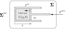
Figure 3: System of an ideal gas confined in a cylinder by a piston

Example: circuits with entropy production.

Let us consider the L-C-R circuit with voltage source $V$ in Figure 2 and recall that the configuration space for the charges is $Q=\mathbb{R}^{4}$. The Lagrangian $L:TQ\times\mathbb{R}\to\mathbb{R}$ of the system is given by $L(\mathbf{q},\mathbf{\dot{q}},S)=\frac{1}{2}L(\dot{q}_{L})^{2}-\frac{1}{2C}(q_{C})^{2}-U(\mathbf{q},S),$ where $U(\mathbf{q},S)$ is the internal energy. Recall that $\Delta_{Q}\subset TQ$ is a constraint distribution associated with the KCL constraints in (2) and also that $F^{\rm fr}(\mathbf{q},\mathbf{\dot{q}},S):=V=-R(\mathbf{q},S)f_{R}$, where $R(\mathbf{q},S)=R$ is a resistive constant. The equations of motion are given by (13), which take the form

$$\begin{split}L\ddot{q}_{L}=V+Rf_{R},\quad R\dot{q}_{R}=\frac{1}{C}q_{C},\quad\dot{q}_{C}=\dot{q}_{L}-\dot{q}_{R},\quad\dot{S}=\frac{1}{T}R\dot{q}_{R}^{2},\end{split}$$

where $T=\frac{\partial U}{\partial S}$ denotes the temperature and $e_{V}=-V$.

3.3 Variational formulation for non-simple thermodynamic systems

Consider a general finite dimensional non-simple thermodynamic system $\boldsymbol{\Sigma}$ where we assume that $\boldsymbol{\Sigma}$ can be decomposed into $P$ subsystems $\boldsymbol{\Sigma}_{k},\;k=1,...,P$, i.e., $\boldsymbol{\Sigma}=\cup_{k=1}^{P}\boldsymbol{\Sigma}_{k}$. For brevity, suppose that each subsystem $\boldsymbol{\Sigma}_{k}$ has a single compartment with a single entropy $S_{k}\in\mathbb{R}$ and with mechanical variables $\mathbf{q}_{k}\in Q_{k}$. Hence the state variables for each $\boldsymbol{\Sigma}_{k}$ are

$$(\mathbf{q}_{k},\dot{\mathbf{q}}_{k},S_{k},)\in TQ_{k}\times\mathbb{R},\quad k=1,...,P.$$ (15)

We write $L_{k}:TQ_{k}\times\mathbb{R}\rightarrow\mathbb{R}$ the Lagrangian of the $k$-th subsystem $\boldsymbol{\Sigma}_{k}$, $k=1,...,P$. We assume that there are nonholonomic constraints given by distributions $\Delta_{Q_{k}}\subset TQ_{k}$ and we also assume that there exists an interconnection constraint $\Sigma_{Q}\subset TQ$ among the subsystems so that we can define the kinematic constraint $\Delta_{Q}=(\Delta_{Q_{1}}\times\cdots\times\Delta_{Q_{P}})\cap\Sigma_{Q}\subset TQ$.

Note that the non-simple system $\boldsymbol{\Sigma}$ can be considered as an interconnected system of $P$ simple systems with the state space $T(Q_{1}\times...\times Q_{P})\times\mathbb{R}^{P}$, as illustrated in Figure 4, where each subsystem $\boldsymbol{\Sigma}_{k}$ is a simple thermodynamic system with the configuration space $Q_{k}$, which is nothing but a primitive system in the sense of Kron. This type of non-simple interconnected systems is a natural extension of the class of an interconnected mechanical system in [19] in the sense that it also includes the irreversible processes due to friction and heat conduction.

Figure 4: Non-simple interconnected system

3.3.1 Variational formulation for systems with friction and heat conduction

Besides the friction forces $\mathbf{F}^{\rm fr}_{k}:TQ_{k}\times\mathbb{R}\rightarrow T^{*}Q_{k}$ associated to each subsystems, we also need to introduce the entropy fluxes $J_{k\ell}$ associated to the heat exchange between subsystems $\boldsymbol{\Sigma}_{k}$ and $\boldsymbol{\Sigma}_{\ell}$, where we assume $J_{k\ell}=J_{\ell k}$.

Thermodynamic displacements associated to heat exchange.

An essential ingredient in the variational formulation of thermodynamics is the notion of thermodynamic displacement associated to an irreversible process. In general, the thermodynamic displacement associated to an irreversible process $\alpha$ with thermodynamic force $X^{\alpha}$ is a variable $\Lambda^{\alpha}$ such that its time rate of change satisfies $\dot{\Lambda}^{\alpha}=X^{\alpha}$, as defined in [9, 10, 13].

For the irreversible process of heat exchange such thermodynamic displacements are given by the variables $\Gamma^{k}$ which satisfy $\dot{\Gamma}^{k}=T^{k}$ with $T^{k}$ the temperature of $\boldsymbol{\Sigma}_{k}$. Note that $\Gamma^{k}$ is the thermal displacement that was used in [15], which was initially coined by [32]. See §3.3.2 for other examples of thermodynamic displacement. The introduction of $\Gamma^{k}$ is accompanied with the introduction of an entropy variable $\Sigma_{k}$, usually distinct from $S_{k}$. The physical meaning of $\Sigma_{k}$ will be explained below.

Variational formulation.

Let us consider the variational formulation for a thermodynamic system with friction and heat conduction, in which the total Lagrangian is given by

$$L:TQ\times\mathbb{R}^{P}\rightarrow\mathbb{R},\qquad L(\mathbf{q},\dot{\mathbf{q}},S_{1},...,S_{P})=\sum_{k=1}^{P}L_{k}(\mathbf{q}_{k},\dot{\mathbf{q}}_{k},S_{k}),$$

with $Q=Q_{1}\times...\times Q_{P}$.

Theorem 3.2 (Variational formulation for non-simple thermodynamic systems).

The following statements are equivalent:

• The curves $\mathbf{q}(t)=(\mathbf{q}_{1}(t),...,\mathbf{q}_{P}(t))$ and $S_{1}(t),...,S_{P}(t)$ are critical for the action functional

  $$\delta\int_{t_{1}}^{t_{2}}\left[L(\mathbf{q},\dot{\mathbf{q}},S_{1},...,S_{P})+\sum_{k=1}^{P}\dot{\Gamma}^{k}(S_{k}-\Sigma_{k})\right]{\rm d}t=0,$$ (16)

  subject to the kinematic constraints

  $$\dot{\mathbf{q}}\in\Delta_{Q}(\mathbf{q}),\qquad\frac{\partial L}{\partial S_{k}}\dot{\Sigma}_{k}=\left<\mathbf{F}_{k}^{\rm fr},\dot{\mathbf{q}}_{k}\right>+\sum_{\ell}J_{k\ell}\dot{\Gamma}^{\ell},\;k=1,...,P$$ (17)

  and for variations subject to the variational constraints

  $$\delta{\mathbf{q}}\in\Delta_{Q}(\mathbf{q}),\qquad\frac{\partial L}{\partial S_{k}}\delta\Sigma_{k}=\left<\mathbf{F}^{\rm fr}_{k},\delta\mathbf{q}_{k}\right>+\sum_{\ell}J_{k\ell}\delta\Gamma^{\ell},\;k=1,...,P$$ (18)

  with $\delta\mathbf{q}(t_{1})=\delta\mathbf{q}(t_{2})=0$.

• The curves $\mathbf{q}(t)=(\mathbf{q}_{1}(t),...,\mathbf{q}_{P}(t))$ and $S_{1}(t),...,S_{P}(t)$ are solutions of the system of equations

  $$\left\{\begin{array}[]{l}\displaystyle\vspace{0.2cm}\frac{d}{dt}\frac{\partial L}{\partial\dot{\mathbf{q}}}-\frac{\partial L}{\partial\mathbf{q}}-\mathbf{F}^{\rm fr}(\mathbf{q},\dot{\mathbf{q}},S_{1},...,S_{P})\in\Delta_{Q}^{\circ}(\mathbf{q}),\\ \displaystyle\dot{\mathbf{q}}\in\Delta_{Q}(\mathbf{q}),\qquad\frac{\partial L}{\partial S_{k}}\dot{S}_{k}=\left<\mathbf{F}_{k}^{\rm fr},\dot{\mathbf{q}}_{k}\right>+\sum_{\ell}J_{k\ell}\left(\frac{\partial L}{\partial S_{k}}-\frac{\partial L}{\partial S_{\ell}}\right),\;k=1,...,P.\end{array}\right.$$ (19)

We recall that the kinematic constraint $\Delta_{Q}$ on the total configuration space $Q=Q_{1}\times....\times Q_{P}$ is built from the nonholonomic constraints $\Delta_{Q_{k}}$ within each subsystem $\boldsymbol{\Sigma}_{k}$ and from the interconnection constraints $\Sigma_{Q}$ among each subsystems as $\Delta_{Q}=(\Delta_{Q_{1}}\times\cdots\times\Delta_{Q_{P}})\cap\Sigma_{Q}\subset TQ$.

The derivation of the final system of equations (19) from (16)–(18) is obtained by noting the two following conditions associated to the variations $\delta S_{k}$ and $\delta\Gamma^{k}$ when applying (16)–(18):

$$\delta S_{k}:\;\;\frac{\partial L}{\partial S_{k}}=-\dot{\Gamma}^{k},\qquad\delta\Gamma^{k}:\;\;\dot{S}_{k}=\dot{\Sigma}_{k}+\sum_{\ell}J_{k\ell}.$$ (20)

The first condition states that $\Gamma^{k}$ indeed corresponds to the thermal displacement, while the second condition defines the entropy variable $\Sigma_{k}$ in terms of $S_{k}$ and the entropy fluxes. The second condition is related to the Prigogine equation

$${\rm d}S={\rm d}_{i}S+{\rm d}_{e}S$$ (21)

as we shall see later. We note that $\dot{\Gamma}^{k}$ and $\dot{\Sigma}_{k}$ ultimately cancel in the final form of the equations.

In the first equation of (19) we have defined $\mathbf{F}^{\rm fr}=(\mathbf{F}^{\rm fr}_{1},...,\mathbf{F}^{\rm fr}_{P})$. We recall that the distribution $\Delta_{Q}\subset TQ$ is defined by $\Delta_{Q}=(\Delta_{Q_{1}}\times...\times\Delta_{Q_{P}})\cap\Sigma_{Q}$, hence the first and second equations can be equivalently written as

$$(\dot{\mathbf{q}}_{1},...,\dot{\mathbf{q}}_{P})\in\Sigma_{Q},\quad\qquad\dot{\mathbf{q}}_{k}\in\Delta_{Q_{k}}(\mathbf{q}_{k}),\quad\qquad\frac{d}{dt}\frac{\partial L}{\partial\dot{\mathbf{q}}_{k}}-\frac{\partial L}{\partial\mathbf{q}_{k}}-\mathbf{F}_{k}^{\rm fr}-\mathbf{F}_{k}\in\Delta_{Q_{k}}^{\circ},$$ (22)

$k=1,...,P$, for some interaction forces $(\mathbf{F}_{1},...,\mathbf{F}_{k})\in\Sigma_{Q}^{\circ}$.

Energy balances and the first law.

Let us consider the energy $E_{k}:TQ_{k}\times\mathbb{R}\rightarrow\mathbb{R}$ of the $k$-th subsystem $\boldsymbol{\Sigma}_{k}$ as

$$E_{k}(\mathbf{q}_{k},\mathbf{v}_{k},S_{k})=\left<\frac{\partial L}{\partial\mathbf{v}_{k}},\mathbf{v}_{k}\right>-L(\mathbf{q}_{k},\mathbf{v}_{k},S_{k}).$$ (23)

From the evolution equations (19) one gets the energy balance

$$\frac{d}{dt}E_{k}=\left\langle\mathbf{F}_{k},\dot{\mathbf{q}}_{k}\right\rangle+\sum_{\ell}J_{k\ell}\left(\frac{\partial L}{\partial S_{\ell}}-\frac{\partial L}{\partial S_{k}}\right)=P^{{\rm int}\rightarrow k}_{W}+P_{H}^{\ell\rightarrow k},$$

which allows to identify the mechanical power $P^{{\rm int}\rightarrow k}_{W}$ associated to the work done on the subsystem $\boldsymbol{\Sigma}_{k}$ arising from the interconnection within the total system $\boldsymbol{\Sigma}$, as well as the power $P_{H}^{\ell\rightarrow k}$ associated to the heat transfer from $\boldsymbol{\Sigma}_{\ell}$ to $\boldsymbol{\Sigma}_{k}$. This is nothing else than the first law associated to the $k$-th subsystem, where we note that the work of the friction force $\mathbf{F}^{\rm fr}_{k}$ does not appear since it is an internal force associated to an irreversible process within the $k$-th subsystem.

The total energy balance for $E=\sum_{k}E_{k}$ is found as

$$\frac{d}{dt}E=\sum_{k}\left\langle\mathbf{F}_{k},\dot{\mathbf{q}}_{k}\right\rangle+\sum_{k,\ell}J_{k\ell}\left(\frac{\partial L}{\partial S_{\ell}}-\frac{\partial L}{\partial S_{k}}\right)=0,$$

where we note that the first term vanishes due to the interconnection condition $(\dot{\mathbf{q}}_{1},...,\dot{\mathbf{q}}_{P})\in\Sigma_{Q}$ and $(\mathbf{F}_{1},...,\mathbf{F}_{k})\in\Sigma_{Q}^{\circ}$. In fact the total energy is preserved since the system $\boldsymbol{\Sigma}$ is isolated.

Entropy balances and the second law.

Recalling that $-\frac{\partial L}{\partial S_{k}}=T^{k}$ is the temperature of the $k$-th subsystem, its entropy balance is found from (19) as

$$\dot{S}_{k}=-\frac{1}{T^{k}}\left<\mathbf{F}_{k}^{\rm fr},\dot{\mathbf{q}}_{k}\right>+\sum_{\ell}J_{k\ell}\frac{T^{k}-T^{\ell}}{T^{k}}.$$

It is important to note that the second law does not implies $\dot{S}_{k}\geq 0$ since the $k$-th subsystem is not adiabatically closed. To apply the second law one has to identify the rate of internal (as opposed to total) entropy production. In our variational approach, the rate of internal entropy production is identified with $\dot{\Sigma}_{k}$ and from the second condition (20), one directly obtains the rate of internal entropy production as

$$\dot{\Sigma}_{k}=-\frac{1}{T^{k}}\left<\mathbf{F}_{k}^{\rm fr},\dot{\mathbf{q}}_{k}\right>-\sum_{\ell}J_{k\ell}\frac{T^{\ell}}{T^{k}}.$$

The second law implies $-\frac{1}{T^{k}}\left<\mathbf{F}_{k}^{\rm fr},\dot{\mathbf{q}}_{k}\right>\geq 0$ and $\sum_{\ell}J_{k\ell}\frac{T^{\ell}}{T^{k}}\geq 0$, thus forcing $\mathbf{F}_{k}^{\rm fr}$ to be dissipative forces and $J_{k\ell}$ to be a non-positive state function.

Because the entropy is considered to be an extensive variable, the total entropy of the system is given by $S=\sum_{k=1}^{P}S_{k}$. By summing the entropy balances of each subsystem we get

$$\dot{S}=-\sum_{k=1}^{P}\frac{1}{T^{k}}\left<\mathbf{F}_{k}^{\rm fr},\dot{\mathbf{q}}_{k}\right>+\sum_{k<\ell}^{K}J_{k\ell}\left(\frac{1}{T^{k}}-\frac{1}{T^{\ell}}\right)(T^{k}-T^{\ell}).$$ (24)

Since the total system $\boldsymbol{\Sigma}$ is isolated, the second law imposes $\dot{S}\geq 0$. This is indeed the case from the conditions on $\mathbf{F}^{\rm fr}_{k}$ and $J_{k\ell}$ already found earlier.

In terms of the Prigogine equation (21) these results can be summarized as follows:

$$\boldsymbol{\Sigma}_{k} :\;{\rm d}S_{k}={\rm d}_{i}S_{k}+{\rm d}_{e}S_{k},\quad{\rm d}_{i}S_{k}\geq 0,\;\;{\rm d}_{e}S_{k}\text{ no sign},$$

$$\boldsymbol{\Sigma} :\;{\rm d}S={\rm d}_{i}S+{\rm d}_{e}S,\quad\quad\;\;\,{\rm d}_{i}S\geq 0,\;\;{\rm d}_{e}S=0,$$

where our variational formulation gives the concrete expressions for each of these quantities as

$$\frac{{\rm d}_{i}S_{k}}{{\rm d}t} =\dot{\Sigma}_{k}=-\frac{1}{T^{k}}\left<\mathbf{F}_{k}^{\rm fr},\dot{\mathbf{q}}_{k}\right>-\sum_{\ell}J_{k\ell}\frac{T^{\ell}}{T^{k}},\qquad\frac{{\rm d}_{e}S_{k}}{{\rm d}t}=\sum_{\ell}J_{k\ell},$$

$$\frac{{\rm d}S}{{\rm d}t} =\dot{S}=-\sum_{k=1}^{P}\frac{1}{T^{k}}\left<\mathbf{F}_{k}^{\rm fr},\dot{\mathbf{q}}_{k}\right>+\sum_{k<\ell}^{K}J_{k\ell}\left(\frac{1}{T^{k}}-\frac{1}{T^{\ell}}\right)(T^{k}-T^{\ell}).$$

In particular, the equations ${\rm d}_{i}S_{k}=\dot{\Sigma}_{k}{\rm d}t$ and ${\rm d}S_{k}=\dot{S}_{k}{\rm d}t$ explicitly show the different physical meanings of the two entropy variables $\Sigma_{k}$ and $S_{k}$ used in the variational formulation.

3.3.2 Extensions to matter exchange, chemical reactions, and open systems

The variational formulation for non-simple systems developed in §3.3.1 can be extended to the case in which each subsystem contains several chemical species undergoing chemical reactions, with possible diffusion of the species between the subsystems in addition to heat exchange. This is achieved by introducing the thermodynamic displacements associated to matter transport and chemical reactions. From its general definition as a time integral of the thermodynamic force, the thermodynamic displacement associated to the matter transport of a chemical species $k$ is given by the variable $W^{k}$ such that its time rate of change is the chemical potential $\mu^{k}$ of this species, namely $\dot{W}^{k}=\mu^{k}$. Similarly, the thermodynamic displacement associated to a chemical reaction is such that its time rate of change is the affinity of the reaction. With these concepts, the variational formulation (16)–(18) extends to these cases, while keeping the same structure, see [9], [13]. An appropriate extension of the variational formulation (16)–(18) also allows the treatment of open systems that exchange heat, matter, and kinetic energy with their surroundings, in which case the constraint becomes affine and explicitly time dependent, [12].

3.3.3 Extensions to continuum systems

It is also possible to extend (16)–(18) to continuum systems in order to treat for instance the case of multicomponent reacting heat conducting viscous fluids, [10, 13]. The structure of the variational formulation remains the same, with the phenomenological and variational constraints related as above, and recovers the Hamilton principle of continuum mechanics in absence of irreversibility. This approach is especially useful as a modelling tool for the derivation of thermodynamically consistent models, especially in systems involving constraints in their variational formulations, such as semi-incompressible fluids, [6] or porous media [8], as well as for the derivation of thermodynamically consistent numerical discretization [11, 7].

4 Interconnection of thermodynamic systems

Here we illustrate the variational formulation of interconnected thermodynamic systems by extending the idea of interconnected systems in mechanics. This approach is crucial when studying multiphysical systems, their interconnection, and their thermodynamic consistency. We start by reviewing the case of mechanics, and then develop the case of simple as well as non-simple thermodynamic systems.

4.1 Variational formulation for interconnected mechanical systems

The variational formulation for an interconnected system in mechanics was developed by [19]. Let us see how it can be formulated for the case in which a mechanical system with configuration manifold $Q=Q_{1}\times Q_{2}\ni\mathbf{q}=(\mathbf{q}_{1},\mathbf{q}_{2})$ is decomposed into two mechanical systems $k=1,2$. Here we suppose also that each $k$-th mechanical system, called a primitive system, has constraints $\Delta_{Q_{k}}\subset TQ_{k}$ in which $Q_{k}$ denotes a configuration manifold of the $k$-th primitive system.

The variational formulation for each subsystem $k=1,2$ is given by

$$\delta\int_{t_{0}}^{t_{1}}L_{k}(\mathbf{q}_{k},\dot{\mathbf{q}}_{k}){\rm d}t+\int_{t_{0}}^{t_{1}}\left\langle\mathbf{F}_{k}(\mathbf{q},\dot{\mathbf{q}}),\delta\mathbf{q}_{k}\right\rangle{\rm d}t=0,\quad\delta\mathbf{q}_{k}\in\Delta_{k}(\mathbf{q}_{k}),\quad\text{for}\quad k=1,2$$ (25)

with the condition $\dot{\mathbf{q}}_{k}\in\Delta_{Q_{k}}(\mathbf{q}_{k})\subset T_{\mathbf{q}_{k}}Q_{k}$, where $\mathbf{F}_{k}:TQ\to T^{\ast}Q_{k}$ is the interaction force at the $k$-th boundary. We note that, unlike $L_{k}$, the interaction force $\mathbf{F}_{k}$ is defined on $TQ$ and not on $TQ_{k}$ only. One gets from (25) the equations of motion for each primitive system as

$$\frac{d}{dt}\frac{\partial L_{k}}{\partial\dot{\mathbf{q}}_{k}}-\frac{\partial L_{k}}{\partial\mathbf{q}_{k}}-\mathbf{F}_{k}\in\Delta_{Q_{k}}^{\circ}(\mathbf{q}_{k}),\qquad\dot{\mathbf{q}}_{k}\in\Delta_{Q_{k}}(\mathbf{q}_{k}).$$ (26)

The interconnection of the two mechanical systems is given by imposing some distribution $\Sigma_{Q}\subset T(Q_{1}\times Q_{2})$ such that

$$(\dot{\mathbf{q}}_{1},\dot{\mathbf{q}}_{2})\in\Sigma_{Q},\qquad(\mathbf{F}_{1},\mathbf{F}_{2})\in\Sigma_{Q}^{\circ}.$$ (27)

The dynamics of the interconnected system, given by (26) together with the interconnection condition (27), is equivalently provided by the interconnected variational formulation

$$\delta\int_{t_{0}}^{t_{1}}\left[L_{1}(\mathbf{q}_{1},\dot{\mathbf{q}}_{1})+L_{2}(\mathbf{q}_{2},\dot{\mathbf{q}}_{2})\right]{\rm d}t=0,\quad(\delta\mathbf{q}_{1},\delta\mathbf{q}_{2})\in\Delta_{Q}(\mathbf{q}_{1},\mathbf{q}_{2}),$$ (28)

with the condition $(\dot{\mathbf{q}}_{1},\dot{\mathbf{q}}_{2})\in\Delta_{Q}(\mathbf{q}_{1},\mathbf{q}_{2})$, where we have defined the new distribution

$$\Delta_{Q}:=\left(\Delta_{Q_{1}}\times\Delta_{Q_{2}}\right)\cap\Sigma_{Q}.$$ (29)

Indeed, (28) gives

$$\left(\frac{d}{dt}\frac{\partial L_{1}}{\partial\dot{\mathbf{q}}_{1}}-\frac{\partial L_{1}}{\partial\mathbf{q}_{1}},\frac{d}{dt}\frac{\partial L_{2}}{\partial\dot{\mathbf{q}}_{2}}-\frac{\partial L_{2}}{\partial\mathbf{q}_{2}}\right)\in\Delta_{Q}^{\circ},\qquad(\dot{\mathbf{q}}_{1},\dot{\mathbf{q}}_{2})\in\Delta_{Q}(\mathbf{q}_{1},\mathbf{q}_{2})$$

which is clearly equivalent to (26) and (27) by using (29).

Remark 4.1 (On primitive systems and interaction forces).

In the above, the primitive system seems to be similar to a system with external force, but strictly speaking it is not the same for two reasons. The first reason is that the $k$-th interaction force $\mathbf{F}_{k}^{\rm int}:TQ\to T^{\ast}Q_{k}$ is defined as a map from the tangent bundle $TQ$ of the total space $Q$ to the cotangent bundle of the $k$-th manifold. This means that the primitive system itself is just a piece that is torn apart from the original system and it makes no physical sense by itself alone. In other words, it makes sense as a disconnected piece of the original system that has to be interconnected with other primitive systems to reconstruct the original system. Then, the interconnected system built from the primitive systems does work as a physical system if we correctly interconnect them. This is a natural way for humans to model complicated systems. To reconstruct the full system, we need to assemble them and each part has an appropriate boundary with some other parts that must be bonded. This ingredient to bond with other parts must be the interaction forces and velocities in our case (the modeler knows how to interconnect them because he knows how they were cut from the original system). If the primitive system is a system with an external force, as we have above, then it must make sense by itself alone and then the force must be defined on $TQ_{k}$, i.e., $\mathbf{F}_{k}^{\rm ext}:TQ_{k}\to T^{\ast}Q_{k}$. The second reason is that the interaction forces $\mathbf{F}_{k}^{\rm int}$ must satisfy the interconnection constraints, see (27), and hence they are rather constraint forces than external forces.

Example: L-C circuit.

Let us illustrate the variational setting for interconnected systems given above with an example of the L-C circuit that is decomposed into two disconnected primitive systems as in Figure 5. Let $Z_{1}$ and $Z_{2}$ denote the external ports resulting by tearing the original system. To establish the original circuit in Figure 5, the external ports are interconnected by equating currents across them.

For this example, the primitive system 1 has the configuration space $Q_{1}=\mathbb{R}^{3}$ with local coordinates $\mathbf{q}_{1}=(q_{L_{1}},q_{L_{2}},q_{Z_{1}})$, where $q_{L_{1}},q_{L_{2}}$ and $q_{Z_{1}}$ denote respectively the charges associated to the inductor $L_{1}$, inductor $L_{2}$ and port $Z_{1}$. The primitive system 2 has the configuration space $Q_{2}=\mathbb{R}^{2}$ with local coordinates $\mathbf{q}_{2}=(q_{Z_{2}},q_{C})$, where $q_{Z_{2}}$ is the charge through the port $Z_{2}$ and $q_{C}$ is the charge stored in the capacitor. We have $Q=Q_{1}\times Q_{2}\ni\mathbf{q}=(\mathbf{q}_{1},\mathbf{q}_{2})=(q_{L_{1}},q_{L_{2}},q_{Z_{1}},q_{Z_{2}},q_{C})$.

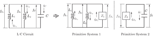
Figure 5: L-C Circuit

Primitive system 1.

Kirchhoff’s circuit law (KCL) is enforced by applying the constraint distribution $\Delta_{Q_{1}}\subset TQ_{1}$ given by

$$\Delta_{Q_{1}}(\mathbf{q}_{1})=\{\dot{\mathbf{q}}_{1}=(\dot{q}_{L_{1}},\dot{q}_{L_{2}},\dot{q}_{Z_{1}})\in T_{\mathbf{q}_{1}}Q_{1}\mid\dot{q}_{L_{1}}-\dot{q}_{L_{2}}-\dot{q}_{Z_{1}}=0\}$$

for each $\mathbf{q}_{1}=(q_{L_{1}},q_{L_{2}},q_{Z_{1}})\in Q_{1}$, where $\dot{\mathbf{q}}_{1}=(\dot{q}_{L_{1}},\dot{q}_{L_{2}}\dot{q}_{Z1})$ denotes the current vector at each $\mathbf{q}_{1}$. The corresponding Kirchhoff’s voltage law (KVL) constraint is described by its annihilator $\Delta_{Q_{1}}^{\circ}$ which reads

$$\Delta_{Q_{1}}^{\circ}(\mathbf{q}_{1})=\{\mathbf{f}_{1}=(f_{L_{1}},f_{L_{2}},f_{Z_{1}})\in T_{\mathbf{q}_{1}}^{\ast}Q_{1}\mid f_{L_{1}}=-f_{L_{2}},-f_{L_{1}}=f_{Z_{1}}\}$$

for each $\mathbf{q}_{1}=(q_{L_{1}},q_{L_{2}},q_{Z_{1}})\in Q_{1}$. The Lagrangian for the primitive circuit 1 is $\mathcal{L}_{1}:TQ_{1}\rightarrow\mathbb{R}$, $\mathcal{L}_{1}(\mathbf{q}_{1},\dot{\mathbf{q}}_{1})=\frac{1}{2}L_{1}\dot{q}_{L_{1}}^{2}+\frac{1}{2}L_{2}\dot{q}_{L_{2}}^{2}.$ The voltage associated to the port $Z_{1}$ is denoted by $f_{Z_{1}}(\mathbf{q},\dot{\mathbf{q}})dq_{Z_{1}}$, giving the interaction voltage field $\mathbf{F}_{1}:TQ\to T^{\ast}Q_{1}$ as $\mathbf{F}_{1}(\mathbf{q},\dot{\mathbf{q}})=(q_{L_{1}},q_{L_{2}},q_{Z_{1}},0,0,f_{Z_{1}}(\mathbf{q},\dot{\mathbf{q}})),$ with $(\mathbf{q},\dot{\mathbf{q}})=(q_{L_{1}},q_{L_{2}},q_{Z_{1}},q_{Z_{2}},q_{C},\dot{q}_{L_{1}},\dot{q}_{L_{2}},\dot{q}_{Z_{1}},\dot{q}_{Z_{2}},\dot{q}_{C})\in TQ$.

With the Lagrangian $\mathcal{L}_{1}$, constraint $\Delta_{Q_{1}}$ and interaction force $\mathbf{F}_{1}$, the equations of motion (26) for the primitive circuit 1 are

$$L_{1}\ddot{q}_{L_{1}}=-\lambda_{1},\qquad L_{2}\ddot{q}_{L_{2}}=-\lambda_{1},\qquad f_{Z_{1}}=\lambda_{1},\qquad\dot{q}_{L_{1}}-\dot{q}_{L_{2}}-\dot{q}_{Z_{1}}=0.$$ (30)

These equations of motion are well defined for each given curve $(\mathbf{q}_{2}(t),\dot{\mathbf{q}}_{2}(t))\in TQ_{2}$.

Primitive system 2.

The KCL space is given by

$$\Delta_{Q_{2}}(\mathbf{q}_{2})=\{\dot{\mathbf{q}}_{2}=(\dot{q}_{Z_{2}},\dot{q}_{C})\in T_{\mathbf{q}_{2}}Q_{2}\mid\dot{q}_{C}-\dot{q}_{Z_{2}}=0\}$$

for each $\mathbf{q}_{2}=(q_{Z_{2}},q_{C})\in Q_{2}$, hence the KVL space described by the annihilator $\Delta_{2}^{\circ}(\mathbf{q}_{2})$ is found as

$$\Delta^{\circ}_{Q_{2}}(\mathbf{q}_{2})=\{\mathbf{f}_{2}=(f_{Z_{2}},f_{C})\in T_{\mathbf{q}_{2}}^{\ast}Q_{2}\mid-f_{C}=f_{Z_{2}}\}.$$

The Lagrangian for the primitive circuit 2 is $\mathcal{L}_{2}:TQ_{2}\to\mathbb{R}$, $\mathcal{L}_{2}=\frac{1}{2C}q_{C}^{2}.$ Given the voltage $f_{Z_{2}}(\mathbf{q},\dot{\mathbf{q}})dq_{Z_{2}}$ associated to the port $Z_{2}$, the interaction voltage field follows as $F_{2}(\mathbf{q},\dot{\mathbf{q}})=(q_{Z_{2}},q_{C},f_{Z_{2}}(\mathbf{q},\dot{\mathbf{q}}),0).$

With the Lagrangian $\mathcal{L}_{2}$, constraint $\Delta_{Q_{2}}$ and interaction force $\mathbf{F}_{2}$, the equation of motion (26) of the primitive system 2 are

$$\begin{split}\dot{q}_{C}-\dot{q}_{Z_{2}}=0,\quad-\frac{q_{C}}{C}=f_{Z_{2}}(\mathbf{q},\dot{\mathbf{q}}).\end{split}$$ (31)

These equations of motion are well defined for each given curve $(\mathbf{q}_{1}(t),\dot{\mathbf{q}}_{1}(t))\in TQ_{1}$.

The interconnected system.

The interconnection of the two primitive systems is given by imposing the equality of currents across the ports, which results in the distribution $\Sigma_{Q}$ on $Q=Q_{1}\times Q_{2}$ given by

$$\Sigma_{Q}=\{(\dot{q}_{L_{1}},\dot{q}_{L_{2}},\dot{q}_{Z_{1}},\dot{q}_{Z_{2}},\dot{q}_{C})\in TQ\mid\dot{q}_{Z_{1}}=\dot{q}_{Z_{2}}\},$$

with the annihilator

$$\Sigma_{Q}^{\circ}=\{(0,0,f_{Z_{1}},f_{Z_{2}},0)\in T^{\ast}Q\mid f_{Z_{1}}+f_{Z_{2}}=0\}.$$

In this way, the current (velocity) $\dot{\mathbf{q}}_{\rm int}=(\mathbf{q}_{L_{1}},\mathbf{q}_{L_{2}},\mathbf{q}_{Z_{1}},\mathbf{q}_{Z_{2}},\mathbf{q}_{C})$ and voltage (force) $\mathbf{f}_{\rm int}=(0,0,f_{Z_{1}},f_{Z_{2}},0)$ at the boundaries must satisfy the constraint $(\dot{\mathbf{q}}_{\rm int},\mathbf{f}_{\rm int})\in\Sigma_{Q}\oplus\Sigma_{Q}^{\circ}$, see (27).

The equations of motion for the interconnected dynamical system are provided by the system of equations for each primitive systems (30) and (31) together with the interconnection condition $\dot{q}_{Z_{1}}=\dot{q}_{Z_{2}}$ and $f_{Z_{1}}+f_{Z_{2}}=0$. Hence we finally get the evolution equations

$$L_{1}\ddot{q}_{L_{1}}=-\frac{q_{C}}{C},\quad L_{2}(\ddot{q}_{L_{1}}-\ddot{q}_{C})=-\frac{q_{C}}{C}.$$

As stated in (28), these equations of evolution are also obtained by the variational formulation for the interconnected system in which we employ the new distribution $\Delta_{Q}=(\Delta_{Q_{1}}\times\Delta_{Q_{2}})\times\Sigma_{Q}$ for the variational and kinematic constraints, and we also note that the internal variables $\mathbf{F}_{k},\,k=1,2$ do not appear in the variational condition.

4.2 Variational formulation for interconnected simple thermodynamic systems

The variational formulation of simple thermodynamic systems has been stated in Theorem 3.1. Here, we consider the case in which the Lagrangian $L:TQ\times\mathbb{R}\rightarrow\mathbb{R}$ is split into a mechanical and a thermal part as $L(\mathbf{q},\dot{\mathbf{q}},S)=L_{\rm mech}(\mathbf{q},\dot{\mathbf{q}})-U(S)$.

Interconnected simple systems.

Let us describe how the thermodynamic system can be understood via interconnection. We reticulate the system into two primitive systems, namely, a primitive system 1 with a purely mechanical part $L_{\rm mech}(\mathbf{q},\dot{\mathbf{q}})$ and a primitive system 2 with a purely thermal part $U(S)$. By tearing the system into two parts, the intermediate or boundary variables $\dot{\mathbf{q}},\dot{\bar{\mathbf{q}}}$ and $\mathbf{F}^{\rm int},\bar{\mathbf{F}}^{\rm int}$ appear.

Primitive system 1:

For the primitive system 1, we consider the variational condition

$$\delta\int_{t_{1}}^{t_{2}}L_{\rm mech}\left(\mathbf{q},\dot{\mathbf{q}}\right){\rm d}t+\int_{t_{1}}^{t_{2}}\left\langle\mathbf{F}^{\rm int}\left(\mathbf{q},\dot{\mathbf{q}},\bar{\mathbf{q}},\dot{\bar{\mathbf{q}}},S\right),\delta{\mathbf{q}}\right\rangle{\rm d}t=0,$$

with $\delta\mathbf{q}(t_{1})=\delta\mathbf{q}(t_{2})=0$, yielding the equation

$$\frac{d}{dt}\frac{\partial L_{\rm mech}}{\partial\dot{\mathbf{q}}}-\frac{\partial L_{\rm mech}}{\partial\mathbf{q}}=\mathbf{F}^{\rm int}.$$ (32)

Primitive system 2:

For the primitive system 2, we consider the variational condition

$$\delta\int_{t_{1}}^{t_{2}}\left[-U(S)\right]{\rm d}t+\int_{t_{1}}^{t_{2}}\left\langle\bar{\mathbf{F}}^{\rm int}(\mathbf{q},\dot{\mathbf{q}},\bar{\mathbf{q}},\dot{\bar{\mathbf{q}}},S),\delta{\bar{\mathbf{q}}}\right\rangle{\rm d}t=0,$$

subject to the phenomenological constraint

$$-\frac{\partial U}{\partial S}\dot{S}=\left\langle\mathbf{F}^{\rm fr}(\bar{\mathbf{q}},\dot{\bar{\mathbf{q}}},S),\dot{\bar{\mathbf{q}}}\right\rangle,$$

and for variations which are subject to the variational constraint

$$-\frac{\partial U}{\partial S}\delta S=\left\langle\mathbf{F}^{\rm fr}(\bar{\mathbf{q}},\dot{\bar{\mathbf{q}}},S),\delta{\bar{\mathbf{q}}}\right\rangle$$

with $\delta{\bar{\mathbf{q}}}(t_{1})=\delta{\bar{\mathbf{q}}}(t_{2})=0$. It gives, the system equations for the primitive system 2 as

$$\left\{\begin{array}[]{l}\displaystyle\vspace{0.2cm}\bar{\mathbf{F}}^{\rm int}+\mathbf{F}^{\rm fr}=0,\\ \displaystyle-\frac{\partial U}{\partial S}\dot{S}=\left\langle\mathbf{F}^{\rm fr}(\bar{\mathbf{q}},\dot{\bar{\mathbf{q}}},S),\dot{\bar{\mathbf{q}}}\right\rangle.\end{array}\right.$$ (33)

Interconnection constraints:

The interconnection constraints between the primitive systems 1 and 2 are given by

$$\dot{\mathbf{q}}=\dot{\bar{\mathbf{q}}},\quad\mathbf{F}^{\rm int}+\bar{\mathbf{F}}^{\rm int}=0,$$ (34)

which indeed fits into the setting (27) with the distribution $\Sigma_{Q}=\{(\dot{\mathbf{q}},\dot{\bar{\mathbf{q}}},\dot{S})\mid\dot{\mathbf{q}}=\dot{\bar{\mathbf{q}}}\}$ for $Q=Q_{1}\times Q_{2}\times\mathbb{R}$. In this case, the interconnection constraints imply Newton’s third law of action and reaction.

Juxtaposing the equations of the primitive systems 1 and 2, namely, equations (32) and (33) together with the interconnection constraints (34) and eliminating the intermediate variables, the total system of equations is obtained as

$$\left\{\begin{array}[]{l}\displaystyle\vspace{0.2cm}\frac{d}{dt}\frac{\partial L_{\rm mech}}{\partial\dot{\mathbf{q}}}-\frac{\partial L_{\rm mech}}{\partial\mathbf{q}}=\mathbf{F}^{\rm fr}(\mathbf{q},\dot{\mathbf{q}},S),\\ \displaystyle-\frac{\partial U}{\partial S}\dot{S}=\left\langle\mathbf{F}^{\rm fr}(\mathbf{q},\dot{\mathbf{q}},S),\dot{\mathbf{q}}\right\rangle.\end{array}\right.$$ (35)

Example: mass-spring-friction system.

A classical example is the mass-spring system with friction whose Lagrangian is $L(q,\dot{q},S)=L_{\rm mech}(q,\dot{q})-U(S)=\frac{1}{2}M\dot{q}^{2}-\frac{1}{2}Kq^{2}-U(S)$, with $M$ is the mass, $K$ is the spring constant, and $U(S)$ is the internal energy. By using (13), in which the external force and the constraint $\Delta_{Q}$ are absent, the equations of motion of the system are given by

$$M\ddot{q}+Kq=F^{\rm fr}(q,\dot{q},S),\quad-\frac{\partial U}{\partial S}\dot{S}=F^{\rm fr}(q,\dot{q},S)\dot{q},$$ (36)

with the friction force $F^{\rm fr}(q,\dot{q},S)=-R(q,S)\dot{q}$ for some friction coefficient $R>0$.

Juxtaposing the system equations of the primitive systems 1 and 2, namely, equations (32) and (33) together with the interconnection constraints, we get the system:

$$\begin{split}&M\ddot{q}+Kq=F^{\rm int}(q,\bar{q},\dot{q},\dot{\bar{q}},S),\\ &\bar{F}^{\rm int}(q,\bar{q},\dot{q},\dot{\bar{q}},S)+F^{\rm fr}(\bar{q},\dot{\bar{q}},S)=0,\quad\displaystyle-\frac{\partial U}{\partial S}\dot{S}=F^{\rm fr}(\bar{q},\dot{\bar{q}},S)\dot{\bar{q}},\\ &\dot{q}=\dot{\bar{q}},\quad F^{\rm int}(q,\bar{q},\dot{q},\dot{\bar{q}},S)+\bar{F}^{\rm int}(q,\bar{q},\dot{q},\dot{\bar{q}},S)=0,\end{split}$$

from which the equations of motion (36) are obtained by eliminating intermediate variables.

4.3 Variational formulation for interconnected non-simple thermodynamic systems

Let us consider the interconnection for the case of non-simple systems, which are thermodynamic systems with several entropies. We focus on the internal process of heat exchange.

4.3.1 Thermodynamic systems with heat exchange

In order to illustrate the theory in simpler terms, we first develop the case of pure heat exchange, without any mechanical parts. We thus consider a non-simple adiabatically closed system experiencing heat conduction between two compartments, see Figure 6, where $S_{k},T^{k},\Gamma^{k},\;k=1,2$ denote entropy, temperature, and thermal displacement of the $k$-th compartment. As earlier, we denote by $J_{k\ell}$, $k,\ell=1,2$, $k\neq\ell$ the entropy fluxes.

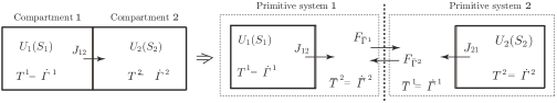
Figure 6: Non-simple closed system experiencing heat conduction between two compartments

The Lagrangian for each primitive system reduces to the internal energy for each compartment, so that $L_{k}(S_{k})=-U_{k}(S_{k})$, $k=1,2$. By tearing the original system into two primitive systems, we need to consider the intermediate thermodynamic forces $(F_{\bar{\Gamma}^{1}},F_{\bar{\Gamma}^{2}})$ dual to $(\dot{\bar{\Gamma}}^{1},\dot{\bar{\Gamma}}^{2})$ at the boundary of the two primitive systems.

Primitive system 1.

The variational condition for primitive system 1 is given as

$$\delta\int_{t_{1}}^{t_{2}}\!\Big{[}L_{1}\left(S_{1}\right)+\dot{\Gamma}^{1}(S_{1}-\Sigma_{1})\Big{]}{\rm d}t+\int_{t_{1}}^{t_{2}}\left(F_{\Gamma^{1}}\delta{\Gamma^{1}}+F_{\bar{\Gamma}^{2}}\delta{\bar{\Gamma}^{2}}\right){\rm d}t=0,$$

under the phenomenological constraint and variational constraint

$$\frac{\partial L_{1}}{\partial S_{1}}\dot{\Sigma}_{1}=J_{12}\dot{\bar{\Gamma}}^{2},\qquad\frac{\partial L_{1}}{\partial S_{1}}\delta\Sigma_{1}=J_{12}\delta{\bar{\Gamma}}^{2},$$

with $\delta\Gamma^{1}(t_{k})=\delta\bar{\Gamma}^{2}(t_{k})=0$, $k=1,2$.

Taking the variations we get

$$\vspace{0.2cm}\delta S_{1}:\;\dot{\Gamma}^{1}=-\frac{\partial L_{1}}{\partial S_{1}},\qquad\delta\Gamma^{1}:\;\dot{S}_{1}=\dot{\Sigma}_{1}+F_{\Gamma^{1}},\qquad\delta\bar{\Gamma}^{2}:\;J_{12}+F_{\bar{\Gamma}^{2}}=0,$$ (37)

while the phenomenological constraint gives

$$\frac{\partial L_{1}}{\partial S_{1}}(\dot{S}_{1}-F_{\Gamma^{1}})=J_{12}\dot{\bar{\Gamma}}^{2}.$$ (38)

Primitive system 2.

Similarly, the variational condition for primitive system 2 is given as

$$\delta\int_{t_{1}}^{t_{2}}\!\Big{[}L_{2}\left(S_{2}\right)+\dot{\Gamma}^{2}(S_{2}-\Sigma_{2})\Big{]}{\rm d}t+\int_{t_{1}}^{t_{2}}\left(F_{\Gamma^{2}}\delta{\Gamma^{2}}+F_{\bar{\Gamma}^{1}}\delta{\bar{\Gamma}^{1}}\right){\rm d}t=0,$$

under the phenomenological constraint and variational constraint

$$\frac{\partial L_{2}}{\partial S_{2}}\dot{\Sigma}_{2}=J_{21}\dot{\bar{\Gamma}}^{1},\qquad\frac{\partial L_{2}}{\partial S_{2}}\delta\Sigma_{2}=J_{21}\delta{\bar{\Gamma}}^{1},$$

with $\delta\Gamma^{2}(t_{k})=\delta\bar{\Gamma}^{1}(t_{k})=0$, $k=1,2$.

Taking the variations, we get

$$\vspace{0.2cm}\delta S_{2}:\;\dot{\Gamma}^{2}=-\frac{\partial L_{2}}{\partial S_{2}},\qquad\delta\Gamma^{2}:\;\dot{S}_{2}=\dot{\Sigma}_{2}+F_{\Gamma^{2}},\qquad\delta\bar{\Gamma}^{1}:\;J_{21}+F_{\bar{\Gamma}^{1}}=0,$$ (39)

while the phenomenological constraint gives

$$\frac{\partial L_{2}}{\partial S_{2}}(\dot{S}_{2}-F_{\Gamma^{2}})=J_{21}\dot{\bar{\Gamma}}^{1}.$$ (40)

Interconnection constraints.

The interconnection of the two systems is given by imposing the equality of the temperatures, thereby giving the interconnection constraint $\Sigma_{\rm heat}$ as

$$\Sigma_{\rm heat}:=\left\{(\dot{\Gamma}^{1},\dot{\bar{\Gamma}}^{2},\dot{\bar{\Gamma}}^{1},\dot{\Gamma}^{2})\;\middle|\;\dot{\Gamma}^{1}=\dot{\bar{\Gamma}}^{1},\;\;\dot{\bar{\Gamma}}^{2}=\dot{\Gamma}^{2}\right\}$$ (41)

from which its annihilator is obtained as

$$\Sigma_{\rm heat}^{\circ}:=\left\{(F_{\Gamma^{1}},F_{\bar{\Gamma}^{2}},F_{\bar{\Gamma}^{1}},F_{\Gamma^{2}})\;\middle|\;F_{\Gamma^{1}}+F_{\bar{\Gamma}^{1}}=0,\;\;F_{\bar{\Gamma}^{2}}+F_{\Gamma^{2}}=0\right\}.$$ (42)

Juxtaposing the equations of the primitive systems 1 and 2, namely, equations (37)–(40) together with the interconnection constraints (41) and (42) and eliminating the intermediate variables, yields the total system equations for heat exchange between two compartments; namely, one eventually gets the system

$$T^{1}\dot{S}_{1}=J_{12}(T^{1}-T^{2}),\qquad T^{2}\dot{S}_{2}=J_{12}(T^{2}-T^{1}),$$

where we recall that $J_{12}=J_{21}$ is a priori assumed as before. This approach also yields the variational formulation of the total system as an interconnected system of the two primitive systems, by adding the two action functionals, taking into account of both constraints as well as the variational constraint for interconnection $\delta{\Gamma}=(\delta{\Gamma}^{1},\delta{\bar{\Gamma}}^{2},\delta{\bar{\Gamma}}^{1},\delta{\Gamma}^{2})\in\Sigma_{\rm heat}$.

4.3.2 Thermodynamic systems with mechanical interactions and heat exchange

We consider now the case of an interconnected non-simple system with both mechanical interactions and heat exchange.

The primitive systems that we consider are simple systems with a mechanical and a thermal part, also with possible mechanical and thermal interactions with their surrounding. Such systems themselves can be further decomposed as in §4.2, however we consider each of them here as one primitive.

For simplicity, we consider the case of only two subsystems ($P=2$) but we can easily generalize to the case of any number of subsystems in the context of interconnected systems. The Lagrangians of the primitive systems are $L_{k}:TQ_{k}\times\mathbb{R}\rightarrow\mathbb{R}$, $k=1,2$ and we suppose the possible occurrence of nonholonomic mechanical constraints $\Delta_{Q_{k}}\subset TQ_{k}$, $k=1,2$. A particular case of such a system is the celebrated piston problem, [16]; see Figure 7, which will be considered as an illustrative example later.

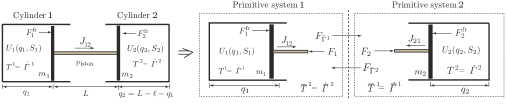
Figure 7: Non-simple closed system with forcing and experiencing heat conduction between two compartments

By combining the approach developed in the pure mechanical case in §4.1 and for heat exchange in §4.3.1 we can state the following variational formulations.

Primitive system 1.

The variational formulation for the primitive system 1 is given as

$$\delta\int_{t_{1}}^{t_{2}}\!\Big{[}L_{1}\left(\mathbf{q}_{1},\dot{\mathbf{q}}_{1},S_{1}\right)+\dot{\Gamma}^{1}(S_{1}-\Sigma_{1})\Big{]}{\rm d}t+\int_{t_{1}}^{t_{2}}\left\langle\mathbf{F}_{1},\delta\mathbf{q}_{1}\right\rangle{\rm d}t+\int_{t_{1}}^{t_{2}}\left(F_{\Gamma^{1}}\delta{\Gamma^{1}}+F_{\bar{\Gamma}^{2}}\delta{\bar{\Gamma}^{2}}\right){\rm d}t=0,$$

subject to the kinematic constraint

$$\dot{\mathbf{q}}_{1}\in\Delta_{Q_{1}}(\mathbf{q}_{1}),\qquad\frac{\partial L_{1}}{\partial S_{1}}\dot{\Sigma}_{1}=\left\langle\mathbf{F}^{\rm fr}_{1},\dot{\mathbf{q}}_{1}\right\rangle+J_{12}\dot{\bar{\Gamma}}^{2},$$

for variations that are subject to the variational constraint

$$\delta\mathbf{q}_{1}\in\Delta_{Q_{1}}(\mathbf{q}_{1}),\qquad\frac{\partial L_{1}}{\partial S_{1}}\delta\Sigma_{1}=\left\langle\mathbf{F}^{\rm fr}_{1},\delta\mathbf{q}_{1}\right\rangle+J_{12}\delta{\bar{\Gamma}}^{2},$$

with $\delta\Gamma^{1}(t_{k})=\delta\bar{\Gamma}^{2}(t_{k})=0$, $k=1,2$.

Taking the variations, we get

$$\vspace{0.2cm}\delta S_{1}:\;\dot{\Gamma}^{1}=-\frac{\partial L_{1}}{\partial S_{1}},\qquad\delta\Gamma^{1}:\;\dot{S}_{1}=\dot{\Sigma}_{1}+F_{\Gamma^{1}},\qquad\delta\bar{\Gamma}^{2}:\;J_{12}+F_{\bar{\Gamma}^{2}}=0,$$ (43)

$$\delta\mathbf{q}_{1}:\;\;\frac{d}{dt}\frac{\partial L_{1}}{\partial\dot{\mathbf{q}}_{1}}-\frac{\partial L_{1}}{\partial\mathbf{q}_{1}}-\mathbf{F}_{1}-\mathbf{F}^{\rm fr}_{1}\in\Delta_{Q_{1}}^{\circ}(\mathbf{q}_{1}),$$

while the kinematic constraints give

$$\dot{\mathbf{q}}_{1}\in\Delta_{Q_{1}}(\mathbf{q}_{1}),\qquad\frac{\partial L_{1}}{\partial S_{1}}(\dot{S}_{1}-F_{\Gamma^{1}})=\left\langle\mathbf{F}^{\rm fr}_{1},\dot{\mathbf{q}}_{1}\right\rangle+J_{12}\dot{\bar{\Gamma}}^{2}.$$ (44)

Primitive system 2.

The variational formulation for the primitive system 2 is given as

$$\delta\int_{t_{1}}^{t_{2}}\!\Big{[}L_{2}\left(\mathbf{q}_{2},\dot{\mathbf{q}}_{2},S_{2}\right)+\dot{\Gamma}^{2}(S_{2}-\Sigma_{2})\Big{]}{\rm d}t+\int_{t_{1}}^{t_{2}}\left\langle\mathbf{F}_{2},\delta\mathbf{q}_{2}\right\rangle{\rm d}t+\int_{t_{1}}^{t_{2}}\left(F_{\Gamma^{2}}\delta{\Gamma^{2}}+F_{\bar{\Gamma}^{1}}\delta{\bar{\Gamma}^{1}}\right){\rm d}t=0,$$

subject to the kinematic constraint

$$\dot{\mathbf{q}}_{2}\in\Delta_{Q_{2}}(\mathbf{q}_{2}),\qquad\frac{\partial L_{2}}{\partial S_{2}}\dot{\Sigma}_{2}=\left\langle\mathbf{F}^{\rm fr}_{2},\dot{\mathbf{q}}_{2}\right\rangle+J_{21}\dot{\bar{\Gamma}}^{1},$$

for variations that are subject to the variational constraint

$$\delta\mathbf{q}_{2}\in\Delta_{Q_{2}}(\mathbf{q}_{2}),\qquad\frac{\partial L_{2}}{\partial S_{2}}\delta\Sigma_{2}=\left\langle\mathbf{F}^{\rm fr}_{2},\delta\mathbf{q}_{2}\right\rangle+J_{21}\delta{\bar{\Gamma}}^{1},$$

with $\delta\Gamma^{2}(t_{k})=\delta\bar{\Gamma}^{1}(t_{k})=0$, $k=1,2$.

Taking the variations, we get

$$\vspace{0.2cm}\delta S_{2}:\;\dot{\Gamma}^{2}=-\frac{\partial L_{2}}{\partial S_{2}},\qquad\delta\Gamma^{2}:\;\dot{S}_{2}=\dot{\Sigma}_{2}+F_{\Gamma^{2}},\qquad\delta\bar{\Gamma}^{1}:\;J_{21}+F_{\bar{\Gamma}^{1}}=0,$$ (45)

$$\delta\mathbf{q}_{2}:\;\;\frac{d}{dt}\frac{\partial L_{2}}{\partial\dot{\mathbf{q}}_{2}}-\frac{\partial L_{2}}{\partial\mathbf{q}_{2}}-\mathbf{F}_{2}-\mathbf{F}^{\rm fr}_{2}\in\Delta_{Q_{2}}^{\circ}(\mathbf{q}_{2}),$$

while the kinematic constraints give

$$\dot{\mathbf{q}}_{2}\in\Delta_{Q_{2}}(\mathbf{q}_{2}),\qquad\frac{\partial L_{2}}{\partial S_{2}}(\dot{S}_{2}-F_{\Gamma^{2}})=\left\langle\mathbf{F}^{\rm fr}_{2},\dot{\mathbf{q}}_{2}\right\rangle+J_{21}\dot{\bar{\Gamma}}^{1}.$$ (46)

Interconnection constraints.

The interconnection of the two systems is given by considering the distribution

$$\Sigma_{\rm int}=\Sigma_{Q}\times\Sigma_{\rm heat},$$ (47)

where $\Sigma_{\rm heat}$ is associated to the equality of temperatures as in (41) and $\Sigma_{Q}\subset T(Q_{1}\times Q_{2})$ describes the mechanical interaction as in §4.1. From this the annihilator is obtained as

$$\!\!\Sigma_{\rm int}^{\circ}:=\left\{(\mathbf{F}_{1},\mathbf{F}_{2},F_{\Gamma^{1}},F_{\bar{\Gamma}^{2}},F_{\bar{\Gamma}^{1}},F_{\Gamma^{2}})\;\middle|\;(\mathbf{F}_{1},\mathbf{F}_{2})\in\Sigma_{Q}^{\circ},\,F_{\Gamma^{1}}+F_{\bar{\Gamma}^{1}}=0,\,F_{\bar{\Gamma}^{2}}+F_{\Gamma^{2}}=0\right\}.$$ (48)

Juxtaposing the equations of the primitive systems 1 and 2, namely, equations (43)–(46) together with the interconnection constraints (47) and (48) and eliminating the intermediate variables, yields the total system equations for the non-simple thermodynamic system, as derived in §3.3.1, see in particular equations (19) and their rewriting in (22) (for $P=2$).

This approach also directly yields the variational formulation of the total system, by adding the two action functionals, taking into account of both constraints as well as the variational constraint for interconnection $(\delta\mathbf{q},\delta{\Gamma})=(\delta\mathbf{q}_{1},\delta\mathbf{q}_{2},\delta{\Gamma}^{1},\delta{\bar{\Gamma}}^{2},\delta{\bar{\Gamma}}^{1},\delta{\Gamma}^{2})\in(\Delta_{Q_{1}}\times\Delta_{Q_{2}}\times\mathbb{R}^{4})\cap\Sigma_{\rm int}$.

The Figure 8 illustrates how the primitive systems $\boldsymbol{\Sigma}_{1}$ and $\boldsymbol{\Sigma}_{2}$ are interconnected to yield the original system $\boldsymbol{\Sigma}$, where $\mathcal{F}_{1}=(\mathbf{F}_{1},F_{\Gamma_{1}},F_{\bar{\Gamma}_{2}})$ and $\mathcal{F}_{2}=(\mathbf{F}_{2},F_{\Gamma_{2}},F_{\bar{\Gamma}_{1}})$ are the interconnection forces.

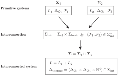
Figure 8: Interconnection in thermodynamics

Example: the piston problem.

As illustrated in Figure 7, consider the piston-cylinder system that is composed of two cylinders connected by a movable piston and suppose that each cylinder contains an ideal gas. Suppose also that the system is isolated. Note that the dynamics of this system is known as the so-called adiabatic piston problem when the piston is adiabatic, and there has been some controversy about the final equilibrium state of this system; see [16] as to the history of this problem.

Now we set $Q_{1}=Q_{2}=\mathbb{R}$ and the Lagrangian and friction force of $k$-th subsystem is

$$L_{k}(q_{k},\dot{q}_{k},S_{k})=\frac{1}{2}m_{k}\dot{q}_{k}^{2}-U_{k}(q_{k},S_{k}),\quad F^{\rm fr}_{k}(q_{k},\dot{q}_{k},S_{k})=-\lambda^{k}(q_{k},S_{k})\dot{q}_{k},\quad k=1,2.$$

The mechanical interconnection constraint is $\Sigma_{Q}=\{(\dot{q}_{1},\dot{q}_{2})\mid\dot{q}_{2}=-\dot{q}_{1}\}$, which follows from the holonomic constraint $q_{2}=L-\ell-q_{1}$, see Figure 7, hence its annihilator is $\Sigma_{Q}^{\circ}=\{(F_{1},F_{2})\mid F_{1}=F_{2}\}$. The interconnection $\Sigma_{\rm heat}$ is associated to the equality of temperatures as in (41). From this, and given $J_{12}=-\kappa$, the conduction coefficient, we can explicitly write the equations (43)–(46) for each subsystems, as well as the interconnection conditions (48). It is easily seen to give the system of differential equations

$$\left\{\begin{array}[]{l}\vspace{0.1cm}(m_{1}+m_{1})\ddot{q}=p_{1}A_{1}-p_{2}A_{2}-(\lambda_{1}+\lambda_{2})\dot{q},\\ \vspace{0.1cm}T^{1}\dot{S}_{1}=\kappa(T^{2}-T^{1})+\lambda_{1}\dot{q}^{2},\\ T^{2}\dot{S}_{2}=\kappa(T^{1}-T^{2})+\lambda_{2}\dot{q}^{2},\end{array}\right.$$

where we define $q:=q^{1}$, which completely describe the evolution of the system. The adiabatic case corresponds to $\kappa=0$.

5 Conclusions

In this paper we have reviewed a variational formulation for nonequilibrium thermodynamics that extends the Hamilton principle of classical mechanics to include irreversible processes, by focusing on the process of friction and heat exchange. We have also proposed a new variational formulation of interconnected systems, where the notion of interconnections in network theory is exclusively extended to nonequilibrium thermodynamics. First we have illustrated that the variational formulation is of the Lagrange-d’Alembert type, in the sense that it consists of a critical curve condition subject to two kind of constraints: a kinematic (phenomenological) constraint and a variational constraint. It is based on the notion of thermodynamic displacement associated to each irreversible process. Second, we have presented a modeling approach to multiphysical complicated thermodynamic systems, in which we first reticulate the system to identify the underlying primitive systems with their interconnection in clear mathematical terms. Further, we have developed such an approach based on the variational formulations, by constructing a variational setting for primitive systems as well as the interconnection conditions in the form of a distribution and its annihilator, $\Sigma_{\rm int}$ and $\Sigma_{\rm int}^{\circ}$, valid for both mechanical and temperature conditions. This setting allows one to concatenate the variational principles in such a way to recover the variational principle of the overall interconnected thermodynamic system. We have illustrated the setting with elementary examples, while we have left the treatment of other process, such as diffusion, chemical reactions, as well as continuum systems, for a future work.

Acknowledgement.

H.Y. is partially supported by JSPS (Grant-in-Aid for Scientific Research 22K03443), JST CREST(JPMJCR1914), Waseda University (SR 2023C-089), and the MEXT “Top Global University Project” at Waseda University.

References

- [1] Biot, M. A. 1975. A virtual dissipation principle and Lagrangian equations in non-linear irreversible thermodynamics, Acad. Roy. Belg. Bull. Cl. Sci. 5 (61), 6–30.
- [2] Biot, M. A. 1984. New variational-Lagrangian irreversible thermodynamics with application to viscous flow, reaction-diffusion, and solid mechanics. Adv. Appl. Mech. 24, 1–91.
- [3] Bloch, A. M. 2003. Nonholonomic Mechanics and Control, volume 24 of Interdisciplinary Applied Mathematics, Springer-Verlag, New York.
- [4] de Groot, S. R., Mazur, P. 1969. Nonequilibrium Thermodynamics, North-Holland.
- [5] Desoer, C. A., Kuh, E. S. 1969. Basic Circuit Theory, McGraw-Hill.
- [6] Eldred, C., Gay-Balmaz, F. 2021. Thermodynamically consistent semi-compressible fluids: a variational perspective, Journal of Physics A: Mathematical and Theoretical, 54, 345701.
- [7] Gawlik, E. S., Gay-Balmaz, F. 2022. Variational and thermodynamically consistent finite element discretization for heat conducting viscous fluids, arXiv:2211.08745v1
- [8] Gay-Balmaz, F., Putkaradze, V. 2022. Variational geometric approach to the thermodynamics of porous media, Zeitschrift für Angewandte Mathematik und Mechanik, accepted.
- [9] Gay-Balmaz, F., Yoshimura, H. 2017. A Lagrangian variational formalism for nonequilibrium thermodynamics. Part I: discrete systems, J. Geom. Phys., 111, 169–193.
- [10] Gay-Balmaz, F., Yoshimura, H. 2017. A Lagrangian variational formalism for nonequilibrium thermodynamics. Part II: continuum systems, J. Geom. Phys., 111, 194–212.
- [11] Gay-Balmaz, F., Yoshimura, H. 2018. Variational discretization for the nonequilibrium thermodynamics of simple systems, Nonlinearity, 31, 1673.
- [12] Gay-Balmaz, F., Yoshimura, H. 2018. A variational formulation of nonequilibrium thermodynamics for discrete open systems with mass and heat transfer, Entropy, 20(3), 163.
- [13] Gay-Balmaz, F., Yoshimura, H. 2019. From Lagrangian mechanics to nonequilibrium thermodynamics: a variational perspective, Entropy, 21(1), 8.
- [14] Glansdorff, P., Prigogine, I. 1971. Thermodynamic Theory of Structure, Stability, and Fluctuations, Wiley-Interscience.
- [15] Green, A. E., Naghdi, P. M. 1991. A re-examination of the basic postulates of thermomechanics, Proc. R. Soc. London. Series A: Mathematical, Physical and Engineering Sciences, 432, 171–194.
- [16] Gruber, C. 1999. Thermodynamics of systems with internal adiabatic constraints: time evolution of the adiabatic piston, Eur. J. Phys. 20, 259–266.
- [17] Grmela, M. 2014. Contact geometry of mesoscopic thermodynamics and dynamics, Entropy, 16(3), 1652–1686.
- [18] Hall, A. D., Fagen, R. E. 1956. Definition of System. General Systems, the Yearbook of the Society for Advancement of General Systems Theory. 1. 18-28.
- [19] Jacobs, H., Yoshimura, H. 2014. Tensor products of Dirac structures and interconnection in Lagrangian mechanics, J. Geo. Mech. 6(1), 67–98.
- [20] Kondepudi, D., Prigogine, I. 1998. textitModern Thermodynamics. John Wiley & Sons.
- [21] Kron, G. 1963. Diakoptics -The Piecewise Solution of Large-Scale Systems. MacDonald, London.
- [22] Lanczos, C. 1986. The Variational Principles of Mechanics. Dover Publications, New York.
- [23] Machlup, S., Onsager, L. 1953. Fluctuations and irreversible processes, Phys. Rev. 91, 1505–1512.
- [24] Onsager, L., Machlup, S. 1953. Fluctuations and irreversible processes II. Systems with kinetic energy. Phys. Rev. 91, 1512–1515.
- [25] Onsager, L. 1931. Reciprocal relations in irreversible processes I, Phys. Rev. 37, 405–426; Reciprocal relations in irreversible processes II, Phys. Rev. 38, 2265–2279.
- [26] Oster, G. F., Perelson, A. S. 1973. Systems, Circuits and Thermodynamics. Israel journal of chemistry, 11(2-3), 445–478.
- [27] Oster, G. F., Perelson, A. S., Katchalsky, A. 1973. Network thermodynamics: dynamic modelling of biophysical systems, Quarterly Reviews of Biophysics 6(1), 1–134.
- [28] Paynter, H. M. 1961. Analysis and design of engineering systems : class notes for M.I.T. course2.751. Cambridge, Mass. M.I.T. Press.
- [29] Poudel, R. M., McGowan, J. G. 2019. The Dynamics of Human Society Evolution: An Energetics Approach, Seatific Journal 2 (1), 27–42.
- [30] Prigogine, I. 1947. Etude thermodynamique des phénomènes irréversibles. Thesis, Paris: Dunod and Liège: Desoer.
- [31] Stueckelberg, E. C. G., Scheurer P. B. 1974. Thermocinétique Phénoménologique Galiléenne, Birkhäuser.
- [32] von Helmholtz, H. 1884. Studien zur Statik monocyklischer Systeme, Sitzungsberichte der Königlich Preussischen Akademie der Wissenschaften zu Berlin, 159–177.
- [33] Wyatt, J. L., Chua, L. O. 1977. A theory of nonenergic -ports, Circuit Theory and Applications 5, 181-208.
- [34] Yoshimura, H., Marsden, J. E. 2006. Dirac structures in Lagrangian mechanics. Part I: Implicit Lagrangian systems, J. Geom. and Phys. 57, 133–156.