ProtoGate: Prototype-based Neural Networks with Local Feature Selection for Tabular Biomedical Data

Abstract

Tabular biomedical data poses challenges in machine learning because it is often high-dimensional and typically low-sample-size. Previous research has attempted to address these challenges via feature selection approaches, which can lead to unstable performance on real-world data. This suggests that current methods lack appropriate inductive biases that capture patterns common to different samples. In this paper, we propose ProtoGate, a prototype-based neural model that introduces an inductive bias by attending to both homogeneity and heterogeneity across samples. ProtoGate selects features in a global-to-local manner and leverages them to produce explainable predictions via an interpretable prototype-based model. We conduct comprehensive experiments to evaluate the performance of ProtoGate on synthetic and real-world datasets. Our results show that exploiting the homogeneous and heterogeneous patterns in the data can improve prediction accuracy while prototypes imbue interpretability.

1 Introduction

In biomedical research, tabular data is frequently collected [1, 2, 3] for a wide range of applications such as detecting marker genes [4], identifying cancer sub-types [4], and performing survival analysis [5, 6]. Clinical trials, whilst collecting large amounts of high-dimensional data using modern high-throughput sequencing technologies, often consider a small number of patients due to practical reasons [7]. The resulting tabular datasets are thus often high-dimensional and typically low-sample-size (HDLSS). Moreover, given the inherent heterogeneity of biomedical data, important features often vary from sample to sample – even in the same dataset [5, 8]. Such scenarios have proven challenging for current machine learning approaches, including deep tabular models [9, 10, 11, 5, 12, 13].

Previous methods [14, 15, 16, 8, 5] have attempted to address such challenges by performing local feature selection: rather than selecting a general set of important features across all samples, local feature selection methods select specific subsets of features for each sample and these subsets may vary from sample to sample. However, existing methods have three limitations: (i) In many real-world tasks, even simple models – such as an MLP or Lasso – can outperform many existing methods [5]. One reason is the accuracy of current methods can be substantially lower for some classes than other classes, and we illustrate this in Figure 1. (ii) These methods commonly comprise a trainable feature selector to select features and a trainable predictor to make predictions with these features, which can be susceptible to the co-adaptation problem [17, 18, 19]. Because the two components are jointly trained, the predictor can fit the selected features to achieve high accuracy even when these features do not reflect the real data distribution [17]. Consequently, the prediction accuracy is inconsistent with the quality of selected features. For instance, L2X [16] achieves 96% accuracy in digit classification on MNIST by using only one pixel as input [17]. (iii) Current methods [8, 17, 5, 16] are not explainable because they mainly use an MLP-based predictor. This lack of explainability is a major concern in high-stake applications such as medicine [20, 21, 22, 23, 24].

We hypothesise that existing local feature selection methods exhibit subpar performance on biomedical data for two reasons: (i) They lack appropriate inductive biases. These methods mainly make predictions using MLPs, although, in the biomedical domain, the clustering assumption (which states similar samples should belong to the same class [25]) has been shown effective [26, 27, 28, 29, 30]. Based on the clustering assumption, the prototype-based models can perform well on tabular data by classifying the new instances according to their similarities to the existing prototypes. For instance, a simple prototype-based model, such as $k$-means, can outperform complex neural networks with an accurate pre-trained feature selector [5]. (ii) Existing local feature selection models tend to overly emphasize heterogeneity, often neglecting that different samples might share some informative features. The high accuracy of global feature selection models on real-world datasets [13] suggests that informative features can indeed be shared across samples. We believe that effective local feature selection methods should be able to identify both homogeneous and heterogeneous feature patterns across samples, provided the data supports their existence.

We aim to address the challenges of suboptimal performance and opaqueness of local feature selection methods applied to tabular biomedical data. We propose ProtoGate, a novel method which performs local feature selection and makes accurate and explainable predictions in the HDLSS regime.

Firstly, ProtoGate uses a prototype-based predictor without learnable parameters – namely Differentiable K-Nearest Neighbors (DKNN) [31] – which enables explainable predictions. The prototype-based predictor confers ProtoGate two important features: (i) an inductive bias aligned with the clustering assumption in biomedical data; and (ii) consistent evaluations of the quality of selected features throughout the training process, eliminating the possibility of co-adaptation from joint training. Secondly, ProtoGate performs feature selection in a global-to-local manner with an $\ell_{1}$-regularised gating network. The global-to-local design helps ProtoGate consider the homogeneous and heterogeneous patterns across multiple samples.

Our contributions can be summarised as follows:

1. We propose ProtoGate, a novel method which addresses the challenge of high-dimensional and low-sample-size (HDLSS) biomedical data by achieving local feature selection and explainable predictions with a global-to-local feature selector and a prototype-based classifier.

2. We show that ProtoGate generally outperforms 12 benchmark methods on seven real-world biomedical datasets (Section 4.1) while selecting fewer features (Section 4.2), paving the path to more robust and interpretable local feature selection models.

3. We demonstrate that ProtoGate effectively handles the co-adaptation problem with a prototype-based predictor by comparing its performance against nine feature selection benchmark methods on three synthetic datasets (Section 4.4).

(a) Class-wise classification accuracy

(b) Class-wise number of selected features

Figure 1: Illustration of the unstable performance of LSPIN [5] on the lung dataset. (a) The class-wise classification accuracy, with class distribution in the parentheses. (b) The mean number of selected features, displayed on a logarithmic scale. MLP and ProtoGate achieve stable performance, while LSPIN has a large variance in the accuracy and number of selected features across different classes.

2 Related Work

Feature Selection Methods Feature selection is a common technique for improving the accuracy and interpretability of machine learning models on HDLSS datasets. An extensive line of work selects features globally with Lasso-based regularisation [32, 33, 34, 35, 36] or specialised layers in neural networks [13, 37, 38, 39, 40]. However, the global feature selection ignores the heterogeneous nature of biomedical data, leading to insufficient interpretability [5, 8].

Prior studies attend to the heterogeneity between samples by designing local feature selection models that select instance-wise features for explaining a pre-trained predictor [17, 41, 42, 43, 44, 45, 46]. These methods are limited because the post-hoc analysis on feature importance does not improve the performance of pre-trained predictors.

Recent work proposes to select instance-wise features for making predictions [8, 5, 16, 15, 47]. L2X uses mutual information for instance-wise feature selection with Concrete distribution, but it requires specifying the number of selected features [16]. INVASE addresses such limitation by modelling each feature’s mask/gate value with independent Bernoulli distributions [8]. However, both methods utilise computationally expensive gradient estimators: REINFORCE [48] or REBAR [49]. Similar to STG [40], LSPIN/LLSPIN re-formalises the mask/gate value with injected Gaussian noise and extends Localized Lasso [50] with a gating network that can select similar features for similar samples [5]. However, the poor performance of a vanilla KNN on real-world datasets (Table 1) demonstrates that the similarity in the initial high-dimensional feature space is inaccurate because a large proportion of features can be noise for the prediction. In contrast, ProtoGate measures the similarity across samples within an intrinsically interpretable DKNN predictor. The predictor takes the samples after feature selection as input, and thus the similarity is measured in a feature space with fewer dimensions than LSPIN/LLSPIN and Localized Lasso.

Co-adaptation Problem In feature selection, co-adaptation refers to the situation where the model encodes predictions into the feature selection, leading to high accuracy with features that do not reflect the real data distributions [17, 18, 19, 51]. REAL-X proves that co-adaptation can happen in models with jointly trained feature selectors and predictors [17], and addresses this problem by decoupling the training objectives of the feature selector and predictor. But it only provides post-hoc explanations of the feature importance for a predictor trained with all features. In ProtoGate, we propose to address the co-adaptation problem with DKNN, a prototype-based predictor without learnable parameters. The DKNN predictor can consistently evaluate the selected features throughout the training process, eliminating the possibility of co-adaptation from joint training.

3 Method

3.1 Problem Setup

We consider the classification task on tabular biomedical data with $\mathcal{Y}$ classes. Let $X\coloneqq[{\bm{x}}^{(1)},\dots,{\bm{x}}^{(N)}]^{\top}\in\mathbbm{R}^{N\times D}$ be the data matrix consisting of $N$ samples ${\bm{x}}^{(i)}\in\mathbbm{R}^{D}$ with $D$ features, and let $Y\coloneqq[y^{(1)},\dots,y^{(N)}]\in\mathbbm{R}^{N}$ be the corresponding labels. We denote $x^{(i)}_{d}$ as the $d$-th feature of the $i$-th sample. To simplify the notation, we assume all samples in $X$ are used for training.

A common local feature selection model contains two components: (i) an instance-wise feature selector $S_{\mathbf{W}}:\mathbbm{R}^{D}\rightarrow\{0,1\}^{D}$ that takes as input a sample ${\bm{x}}^{(i)}$ and generates a mask ${\bm{s}}^{(i)}\in[0,1]^{D}$ for its features, and (ii) a predictor model $F_{\theta}:\mathbbm{R}^{D}\rightarrow\mathcal{Y}$ which takes as input both the sample ${\bm{x}}^{(i)}$ and the mask ${\bm{s}}^{(i)}$ for prediction:

$$\hat{y^{(i)}}=F_{\theta}\left(S_{\mathbf{W}}({\bm{x}}^{(i)}),{\bm{x}}^{(i)}\right)=F_{\theta}({\bm{x}}^{(i)}\odot{\bm{s}}^{(i)}),$$ (1)

where $\hat{y^{(i)}}$ is the predicted label and $\odot$ is the element-wise multiplication. Here, we define the $d$-th feature is selected if and only if the mask value is positive ($s_{d}^{(i)}>0$).

3.2 Rationale for Model Architecture

We propose ProtoGate as a method for selecting instance-wise features with inductive bias from the prototype-based model, as shown in Figure 2. Instead of predicting the local mask from all features, ProtoGate selects instance-wise features in a global-to-local manner with an $\ell_{1}$-regularised gating network. This allows the feature selector to attend to both homogeneity and heterogeneity across samples. Additionally, ProtoGate leverages the selected features with a prototype-based predictor of DKNN. The DKNN predictor makes explainable predictions and encodes the clustering assumption into feature selection. Without learnable parameters, DKNN can further avoid the co-adaptation problem by providing consistent evaluations for the selected features while training the feature selector. The pseudocode for model training is summarised in Algorithm 1.

Figure 2: The architecture of ProtoGate. (A) Given a sample ${\bm{x}}\in\mathbbm{R}^{D}$, the global-to-local feature selector performs global feature selection in the first layer. The orange dashed lines denote sparsified weights in $\mathbf{W}^{[1]}$ under $\ell_{1}$ regularisation. The neural network then computes the instance-wise mask values $\{s_{d}\}_{d=1}^{D}\in[0,1]^{D}$ with a thresholding function. (B) The mask is applied to the sample for local feature selection by element-wise multiplication. (C) The prototype-based predictor classifies ${\bm{x}}$ by retrieving the $K$ nearest neighbours to the masked sample in base $\mathcal{B}$. The majority class of neighbours is used as the predicted label $\hat{y}$.

Algorithm 1 Training Procedure of ProtoGate

training samples $X\in\mathbbm{R}^{N\times D}$, ground truth labels $Y\in\mathbbm{R}^{N}$, global-to-local feature selector $S_{\mathbf{W}}$, prototype-based classifier $F$, sparsity hyper-parameters ($\lambda_{g}$, $\lambda_{l}$), number of nearest neighbours $K$, total training epochs $E$, learning rate $\alpha$

trained model $S_{\mathbf{W}}$, prototype base $\mathcal{B}$

$\mathbf{W}$ $\leftarrow$ GaussianInitialisation() $\triangleright$ Initialise the weights of feature selector

for $e\leftarrow 1$ to $E$ do

     $\mathcal{B}\leftarrow\{\}$ $\triangleright$ Initialise the prototype base as an empty set

     for $i\leftarrow 1$ to $N$ do $\triangleright$ Construct the prototype base

         ${\bm{x}}_{\text{masked}}^{(i)}\leftarrow{\bm{x}}^{(i)}\odot S_{\mathbf{W}}({\bm{x}}^{(i)})$ $\triangleright$ Select instance-wise features for training samples

         $\mathcal{B}\leftarrow\mathcal{B}\cup\{({\bm{x}}_{\text{masked}}^{(i)},y^{(i)})\}$ $\triangleright$ Add masked sample and its label to the prototype base

     end for

     for $i\leftarrow 1$ to $N$ do

         ${\bm{x}}_{\text{masked}}^{(i)}\leftarrow{\bm{x}}^{(i)}\odot S_{\mathbf{W}}({\bm{x}}^{(i)})$ $\triangleright$ Select instance-wise features for training samples

         $P_{\mathcal{B}}^{(i)}\leftarrow\text{NeuralSort}(\mathcal{B},{\bm{x}}_{\text{masked}}^{(i)})$ $\triangleright$ Compute the permutation matrix for ${\bm{x}}_{\text{masked}}^{(i)}$

         $\hat{y^{(i)}}\leftarrow F(\mathcal{B},{\bm{x}}_{\text{masked}}^{(i)},K)$ $\triangleright$ Classify the query sample with $K$ nearest prototypes

     end for

     $L=\frac{1}{N}\sum_{i=1}^{N}\left(\ell_{\text{pred}}(P_{\mathcal{B}}^{(i)},{\bm{x}}^{(i)},y^{(i)})+R(\mathbf{W}^{[1]},{\bm{s}}^{(i)},\lambda_{g},\lambda_{l})\right)$ $\triangleright$ Compute the training loss

     $\mathbf{W}\leftarrow\mathbf{W}-\alpha\nabla_{\mathbf{W}}L$ $\triangleright$ Update the weights of feature selector

end for

return $S_{\mathbf{W}}$, $\mathcal{B}$

3.3 Global-to-local Feature Selection

The global-to-local feature selector $S_{\mathbf{W}}:\mathbbm{R}^{D}\rightarrow[0,1]^{D}$ (Figure 2 (A)) is a neural network that maps feature values ${\bm{x}}^{(i)}$ into mask values ${\bm{s}}^{(i)}$. The feature selector attends to the homogeneity between samples via applying $\ell_{1}$-regularisation on $\mathbf{W}^{[1]}$, the weights of the first layer. Intuitively, the regularisation can lead to sparse weights in the first layer, which implicitly selects features globally for all samples. The output ${\bm{\mu}}^{(i)}$ from the last layer is thresholded to obtain instance-wise mask values by

$$s_{d}^{(i)}=\max(0,\min(1,\mu_{d}^{(i)}+\epsilon_{d}^{(i)}))$$ (2)

where $\epsilon_{d}^{(i)}$ is the injected noise sampled from Gaussion distribution $\mathcal{N}(0,\sigma^{2})$. The standard deviation $\sigma$ is fixed during training, and it is removed during the inference time for deterministic mask values. With the injected noise, ${\bm{s}}^{(i)}$ can be re-formalised as random vectors with parameters ${\bm{\mu}}^{(i)}$ predicted by a neural network. Therefore, the sparsity regularisation on mask values can be computed by

$$\small R(\mathbf{W}^{[1]},{\bm{s}}^{(i)},\lambda_{g},\lambda_{l})=\lambda_{g}||\mathbf{W}^{[1]}||_{1}+\mathbbm{E}\left[\lambda_{l}||{\bm{s}}^{(i)}||_{0}\right]\!=\!\lambda_{g}||\mathbf{W}^{[1]}||_{1}+\lambda_{l}\sum_{d=1}^{D}\!\left(\frac{1}{2}-\frac{1}{2}\text{erf}(-\frac{\mu_{d}^{(i)}}{\sqrt{2}\sigma})\right)$$ (3)

where $(\lambda_{g},\lambda_{l})$ is a pair of hyper-parameters to balance the effects of global and local feature selection, and $\text{erf}(\cdot)$ is the Gauss error function. The full derivations are available in Appendix B.

3.4 Prototype-based Prediction

The prototype-based predictor $F:\mathbbm{R}^{D}\rightarrow\mathcal{Y}$ is a DKNN model (Figure 2 (C)). The DKNN predictor first constructs a prototype base $\mathcal{B}$ with training samples. After masking the training samples with the mask generated by $S_{\mathbf{W}}(X)$, DKNN retains the masked samples and their labels as prototypes in the base $\mathcal{B}\coloneqq\{(S_{\mathbf{W}}({\bm{x}}^{(i)})\odot{\bm{x}}^{(i)},y^{(i)})\}_{i=1}^{N}$. With the acquired prototypes, the predictor can classify a query sample ${\bm{x}}_{\text{query}}\in X$ by retrieving the base $\mathcal{B}$. The predictor sorts the prototypes by their similarities to the masked query sample with NeuralSort [31], a differentiable relaxed sorting operator. Note that ProtoGate computes the Euclidean distance between samples as the similarity evaluation metric. According to the sorting results, the predictor uses the majority class of the $K$ closest prototypes as the predicted label $\hat{y}_{\text{query}}$. Because the feature selector is learnable, the mask can change and thus the base $\mathcal{B}$ is dynamic over the training time. After training, the prototype base $\mathcal{B}$ is fixed and query samples are from unseen test data.

For each query sample, the loss of prototype-based classification is defined as:

$$\ell_{\text{pred}}(P_{\mathcal{B}}^{\text{query}},{\bm{x}}_{\text{query}},y_{\text{query}})=K-\frac{1}{K}\sum_{j=1}^{K}\sum_{i=1}^{N}\mathbbm{1}\left(y^{(i)}=y_{\text{query}}\right)P_{\mathcal{B}}^{\text{query}}[i,j]$$ (4)

where $P_{\mathcal{B}}^{\text{query}}\in\mathbbm{R}^{N\times N}$ denotes the relaxed permutation matrix and $\mathbbm{1}(\cdot)$ denotes the indicator function. In the permutation matrix, $P_{\mathcal{B}}^{\text{query}}[i,j]$ denotes the possibility that the $i$-th prototype is the $j$-th closest to query sample ${\bm{x}}_{\text{query}}$ under NeuralSort. Among the $K$ nearest prototypes, Equation 4 estimates the number of prototypes that have different labels to ${\bm{x}}_{\text{query}}$. DKNN encodes the clustering assumption into feature selection by encouraging samples of the same class to have similar representations. Additionally, DKNN measures the similarity between masked samples and mitigates the effects of the noisy features in the initial high-dimensional feature space.

3.5 Training Loss

The training loss is comprised of the average classification loss in Equation 4 and the sparsity regularisation in Equation 3:

$$L=\frac{1}{N}\sum_{i=1}^{N}\left(\ell_{\text{pred}}(P_{\mathcal{B}}^{(i)},{\bm{x}}^{(i)},y^{(i)})+R(\mathbf{W}^{[1]},{\bm{s}}^{(i)},\lambda_{g},\lambda_{l})\right)$$ (5)

Because the loss function is fully differentiable, the global-to-local feature selector and the prototype-based predictor can be trained in tandem. The whole model can be optimised with standard gradient-based approaches, such as stochastic gradient descent. We did not observe optimisation issues when training over 3,000 models (Appendix A.4).

4 Experiments

We now evaluate ProtoGate on both synthetic and real-world datasets to substantiate the model design choices. Firstly, we compare ProtoGate against 12 benchmark methods on real-world classification tasks (Section 4.1 and Section 4.2). Secondly, we investigate the impact of the prototype-based predictor by replacing it with a linear or MLP-based prediction head (Section 4.3) and adjusting the number of nearest neighbours (Appendix D). Thirdly, we investigate the impact of the global-to-local feature selector by considering the interplay between global and local feature selection (Section 4.3). Finally, we analyse the co-adaptation problem by considering the performance misalignment between feature selection and classification on the synthetic datasets (Section 4.4). We also provide the comparison of training time in Appendix E.

Real-world datasets. Following [13], we utilise seven HDLSS tabular biomedical datasets. The datasets contain $2000$ – $5966$ features with $62$ – $197$ samples of $2$ – $4$ different classes. We are interested in datasets with much fewer samples than LSPIN [5], which uses $\sim 1,500$ samples. Full descriptions of the real-world datasets are available in Appendix A.1.

Experimental setup. For each dataset, we perform 5-fold cross-validation on 5 different splits, summing up to 25 runs per model. We obtain the validation set by randomly selecting 10% of training data. For each benchmark model, the training loss is a weighted loss, and we perform a hyper-parameter search for model selection on the validation set. Full details about the reproducibility and hyper-parameter tuning are available in Appendix A.5.

Evaluation metrics. We report the results averaged over 25 runs on test sets. (i) For classification, we measure the performance by the mean $\pm$ std test balanced accuracy. (ii) Note that the proportion of selected features varies across samples for local feature selection methods. Therefore, we measure the sparsity of feature selection by the mean $\pm$ std proportion of selected features across samples. (iii) To distinguish between “similar number of selected features” and “similar selected features”, we introduce a new metric: degree of local sparsity $\mathcal{Q}$, which is computed by

$$\mathcal{Q}=\frac{1}{D\cdot N}\sum_{j=1}^{N}\text{card}\left(\bigcup_{i=1}^{N}\text{nonzero}({\bm{s}}^{(i)})-\text{nonzero}({\bm{s}}^{(j)})\right)$$ (6)

where $\text{card}(\cdot)$ returns the cardinality of a set and $\text{nonzero}(\cdot)$ returns the indices of non-zero elements in a vector. $\mathcal{Q}$ measures the difference between the union set of selected features for all samples and the selected features for a specific sample. Intuitively, a non-zero $\mathcal{Q}$ denotes selected features are different across samples, and thus the feature selection is local. For global feature selection, the degree of local sparsity is zero ($\mathcal{Q}\equiv 0$).

ProtoGate implementation. The global-to-local feature selector is flexible on the number of hidden layers, and we implement it as a three-layer feed-forward neural network. The numbers of neurons in the input and output layers are the same as the number of features of the input data and the number of neurons in the hidden layer is set to 100. The feature selector has batch normalisation and $tanh$ activation for all layers. We train the models with a batch size of 64 and utilise an SGD optimiser with a weight decay of $1e-4$. The number of nearest neighbours $K$ is searched in $\{1,2,3,4,5\}$. The global sparsity hyper-parameter $\lambda_{g}$ is searched in $\{1e-4,2e-4,3e-4,4e-4,6e-4\}$, and the local sparsity hyper-parameter $\lambda_{l}$ is set as $1e-3$.

Benchmark methods. We evaluate the classification accuracy of ProtoGate and compare it with several benchmark models, including global feature selection models (LightGBM [52], Random Forest (RF) [53], Lasso [32] and STG [40]) and local feature selection models (TabNet [15], L2X [16], INVASE [8], REAL-X [17] and LSPIN/LLSPIN [5]). Additionally, we also compare ProtoGate with some standard models, including KNN [54] and MLP.

4.1 Classification Performance

Table 1 shows that ProtoGate consistently achieves better than or comparable balanced accuracy to the benchmark models. We compute the average rank across different datasets and ProtoGate ranks first, followed by Lasso. ProtoGate outperforms all other local feature selection models by a clear margin. We also find that the existing local feature selection methods cannot outperform even the simple linear Lasso or vanilla MLPs on HDLSS datasets. Note that REAL-X trains the MLP-based predictor with all features, and thus it achieves comparable performance as the MLP model.

The stable and competitive performance of ProtoGate shows the suitability of the clustering assumption in the biomedical field. Moreover, ProtoGate intrinsically provides explanations for the predictions by explicitly pointing out the $K$ nearest prototypes, while other local feature selection methods can be unexplainable with MLP-based predictors. Poor performance of the vanilla KNN model also demonstrates that a large proportion of features can be irrelevant to the predictions, and thus the similarity in the high-dimensional feature space can introduce noise to feature selection, which can be one reason for the failure of LSPIN and LLSPIN.

In most HDLSS cases, ProtoGate consistently outperforms both Lasso and MLP. The exceptions are the lung, prostate and toxicity datasets, where the ProtoGate accuracy is slightly lower. As mentioned in [13, 5], Lasso and MLP can outperform other feature selection models when they are well-regularised on some datasets, such as the toxicity dataset. Compared with well-regularised Lasso and MLP, the prototype-based predictor could have limited expressivity, resulting in the suboptimal performance of ProtoGate.

Table 1: Evaluation comparison of ProtoGate with 12 benchmark methods on seven real-world tabular biomedical datasets. We report the mean $\pm$ std balanced accuracy (averaged across 25 runs) and average accuracy rank across datasets. A higher rank implies higher accuracy. We highlight the First, Second and Third ranking accuracy for each dataset. ProtoGate consistently ranks Top-3 across datasets and achieves the best overall performance.

Methods	lung	meta-dr	meta-pam	prostate	tcga-2y	toxicity	colon	Avg. Rank
LightGBM	93.42 $\pm$ 5.91	58.23 $\pm$ 8.56	94.98 $\pm$ 5.19	91.38 $\pm$ 5.71	57.09 $\pm$ 7.87	81.98 $\pm$ 6.25	76.60 $\pm$ 11.67	5.71
RF	91.73 $\pm$ 6.61	51.48 $\pm$ 3.41	88.73 $\pm$ 6.24	90.38 $\pm$ 7.31	58.70 $\pm$ 6.84	79.78 $\pm$ 7.10	80.05 $\pm$ 10.37	7.14
KNN	91.06 $\pm$ 7.92	54.64 $\pm$ 7.95	82.79 $\pm$ 9.20	78.78 $\pm$ 6.71	58.83 $\pm$ 7.07	83.86 $\pm$ 12.03	77.33 $\pm$ 5.41	8.00
Lasso	94.47 $\pm$ 3.17	58.58 $\pm$ 9.04	95.15 $\pm$ 2.83	91.18 $\pm$ 6.39	56.99 $\pm$ 6.26	91.86 $\pm$ 5.27	79.40 $\pm$ 8.50	4.29
MLP	95.81 $\pm$ 2.69	54.68 $\pm$ 9.63	95.71 $\pm$ 2.59	87.22 $\pm$ 7.41	55.32 $\pm$ 7.24	93.54 $\pm$ 4.28	80.00 $\pm$ 8.70	5.14
STG	93.30 $\pm$ 6.28	58.15 $\pm$ 8.67	76.13 $\pm$ 8.19	89.38 $\pm$ 5.85	57.04 $\pm$ 5.76	87.95 $\pm$ 5.01	79.55 $\pm$ 10.53	6.29
TabNet	77.65 $\pm$ 11.56	49.18 $\pm$ 15.02	82.66 $\pm$ 7.81	65.66 $\pm$ 9.03	51.58 $\pm$ 8.26	40.06 $\pm$ 12.23	56.75 $\pm$ 7.31	12.00
L2X	50.02 $\pm$ 8.30	52.54 $\pm$ 13.75	62.64 $\pm$ 13.69	61.78 $\pm$ 6.29	52.30 $\pm$ 9.11	31.72 $\pm$ 13.48	57.60 $\pm$ 14.26	12.43
INVASE	91.22 $\pm$ 6.16	$-$	91.70 $\pm$ 6.84	$-$	55.98 $\pm$ 6.45	80.04 $\pm$ 6.60	$-$	9.00
REAL-X	93.27 $\pm$ 4.32	60.01 $\pm$ 7.12	95.59 $\pm$ 3.04	86.75 $\pm$ 6.68	59.30 $\pm$ 7.49	90.79 $\pm$ 4.75	76.75 $\pm$ 12.21	5.14
LLSPIN	70.10 $\pm$ 12.31	56.77 $\pm$ 9.65	95.50 $\pm$ 3.60	88.71 $\pm$ 5.98	57.87 $\pm$ 6.02	81.67 $\pm$ 9.01	79.35 $\pm$ 7.74	7.14
LSPIN	76.92 $\pm$ 9.38	53.98 $\pm$ 8.00	97.18 $\pm$ 3.16	87.75 $\pm$ 6.74	55.95 $\pm$ 7.45	83.47 $\pm$ 8.59	81.30 $\pm$ 7.97	6.71
ProtoGate	93.44 $\pm$ 6.37	60.43 $\pm$ 7.61	95.96 $\pm$ 3.93	90.58 $\pm$ 5.64	61.18 $\pm$ 6.47	92.34 $\pm$ 5.67	81.10 $\pm$ 12.14	2.00

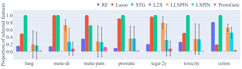
Figure 3: Comparison of the feature selection sparsity on real-world datasets. We report the mean $\pm$ std of the proportion of selected features on test samples, averaged over 25 runs. ProtoGate learns sparser patterns than other methods by a clear margin except for L2X.

4.2 Feature Selection Performance

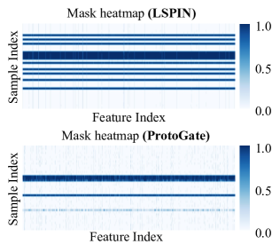
Figure 4: Heatmaps of mask values on the meta-dr dataset. ProtoGate has a sparser feature selection result, since it can better identify the homogeneity across samples.

We compare ProtoGate against both global feature selection methods (RF, Lasso and STG) and local feature selection methods (L2X, LSPIN and LLSPIN). We plot the mean $\pm$ std of the proportion of selected features across samples in Figure 3. The numerical results and full visualisation of selected features are available in Appendix C.

Figure 3 and Figure 4 show that ProtoGate consistently selects fewer features per sample than other benchmark methods, except L2X. Because the performance of L2X is the worst among the 12 benchmark models, we argue that the L2X model does not perform better than ProtoGate on feature selection although it has the fewest selected features. Compared with the rest local feature selection methods, ProtoGate has smaller standard deviations in the proportion of selected features across test samples. Note that this does not mean that ProtoGate selects features globally, because similar proportions of selected features only denote similar numbers of selected features, not necessarily similar selected features (Section 4.3). The sparse feature selection results from ProtoGate demonstrate the effectiveness of global information in feature selection, and the global-to-local process helps ProtoGate attend to both homogeneity and heterogeneity across samples.

4.3 Model Design Ablations

Impact of prototype-based predictor. We now investigate how the prototype-based predictor impacts classification performance. For a fair comparison, we replace the DKNN predictor with a linear head network or an MLP, and then tune the hyper-parameter for global sparsity $\lambda_{g}$ by searching within $\{1e-4,2e-4,3e-4\}$.

As shown in Table 2, the DKNN predictor consistently outperforms other predictors. We attribute the performance improvement to the appropriate inductive bias in prototype-based classification and the reduction in learnable parameters. In ProtoGate, only the feature selector needs training, while other local feature selection methods have learnable predictors with vast amounts of parameters to optimise. We also find that simply combining a global-to-local feature selector and an MLP/linear prediction head does not outperform LSPIN/LLSPIN. This further indicates that a prototype-based predictor is the key to the high accuracy of ProtoGate.

Table 2: Balanced accuracy for different predictors on real-world datasets, averaged over 25 runs. We bold the highest accuracy for each dataset. The prototype-based classifier consistently outperforms linear and MLP predictors on all datasets.

Predictors	lung	meta-dr	meta-pam	prostate	tcga-2y	toxicity	colon
MLP	69.97 $\pm$ 9.17	56.00 $\pm$ 6.37	93.62 $\pm$ 6.04	89.13 $\pm$ 6.36	54.74 $\pm$ 8.11	90.36 $\pm$ 5.61	80.95 $\pm$ 7.77
Linear Head	66.51 $\pm$ 12.45	56.10 $\pm$ 8.95	93.20 $\pm$ 6.18	89.87 $\pm$ 5.80	56.60 $\pm$ 8.20	90.29 $\pm$ 5.93	79.45 $\pm$ 6.23
DKNN	93.44 $\pm$ 6.37	60.43 $\pm$ 7.61	95.96 $\pm$ 3.93	90.58 $\pm$ 5.64	61.18 $\pm$ 6.47	92.34 $\pm$ 5.67	81.10 $\pm$ 12.14

Impact of global-to-local feature selector. In Section 4.2, we discussed how the global-to-local feature selector helps ProtoGate generate a sparser feature selection result. We further examine how different hyper-parameter values of global sparsity $\lambda_{g}$ impact the feature selection behaviour.

Figure 5(a) shows that increasing $\lambda_{g}$ can lead to a lower degree of local sparsity. We also find in Figure 5(b) that ProtoGate achieves the best test accuracy when selecting features locally ($\mathcal{Q}>0$), which aligns with the domain knowledge that heterogeneity across samples is important for accurate predictions on biomedical data. This also suggests that the outstanding performance of ProtoGate is due to its considering both homogeneity and heterogeneity for feature selection.

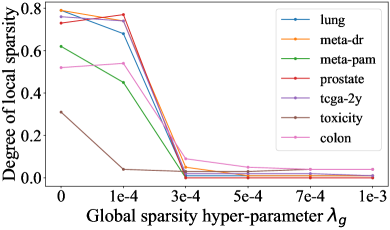
(a) Degree of local sparsity under different $\lambda_{g}$

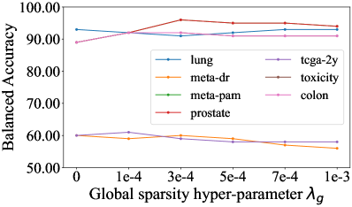
(b) Balanced accuracy under under different $\lambda_{g}$

Figure 5: Comparison of different values of global sparsity hyper-parameter $\lambda_{g}$. (a) The degree of local sparsity averaged over 25 runs. Increasing $\lambda_{g}$ reduces the diversity of selected features between samples. (b) The balanced accuracy averaged over 25 runs. Increasing $\lambda_{g}$ does not guarantee improvement in the prediction accuracy.

Training considerations. ProtoGate can require larger training overhead, mostly for tuning the hyper-parameters compared to some existing models, since we need to consider the interplay between $\lambda_{g}$, $\lambda_{l}$ and $K$. ProtoGate also stores all training samples in the prototype base $\mathcal{B}$, leading to higher memory consumption on large datasets than benchmark methods. Because we mainly focus on the HDLSS datasets, memory consumption is not a major problem in this regime.

4.4 Co-adaptation Analysis

We evaluate ProtoGate and benchmark feature selection models on the synthetic datasets to examine their correctness in feature selection and susceptibility to the co-adaptation problem. We use the same experimental settings as real-world datasets and change the range of hyper-parameter searching for each model to achieve their optimal performance. Following [5, 17], we measure the quality of selected features by computing the F1 score with predicted masks and ground truth masks, and the results are averaged over 25 runs.

Synthetic datasets. We generate three synthetic datasets by adapting the nonlinear datasets used in [5, 8, 17], and the exact data models are described in Appendix A.2. Each dataset has 200 samples of 100 features, which is only 10% of the samples and 10 times more features compared to [5]. All feature values are sampled independently from $\mathcal{N}(0,\mathbf{I})$, where $\mathbf{I}$ is an $100\times 100$ identity matrix. Each dataset has two classes, and we make the data distribution imbalance by generating 50 and 150 samples for two classes respectively.

We purposely design Syn3_(-) to examine the inductive bias in ProtoGate. Note that the absolute value function is an even function. Two samples with opposite values of the same feature are likely to have equal logit values, and then they belong to the same class. However, the opposite values mean a long distance between them, and they should not belong to the same class according to the clustering assumption. Therefore, prototype-based models are expected to perform poorly in this regime. We implement it by adding absolute value function $|x_{9}|$ in the first class of Syn3_(-) to observe the performance degradation in ProtoGate.

Results. On Syn1₍₊₎ and Syn2₍₊₎, ProtoGate achieves better or comparable performance in feature selection and classification than benchmark methods. On Syn3_(-), ProtoGate performs poorly as expected. Although Syn1₍₊₎ and Syn2₍₊₎ also contain even functions like square and absolute value, they also have many other informative features that do not utilise the even functions to compute logit value. Therefore, the side effect of even functions is diluted in Syn1₍₊₎ and Syn2₍₊₎.

We also find LSPIN achieves the highest accuracy on Syn1₍₊₎, but has poor F1${}_{\text{selec}}$ in the selected features, denoting a severe problem of co-adaptation between the feature selector and predictor. In other words, LSPIN simply overfits the dataset without correctly identifying the informative features, making the feature selection results meaningless. In contrast, ProtoGate has consistently non-positive rank differences between F1${}_{\text{selec}}$ and ACC${}_{\text{pred}}$, showing that the co-adaptation does not occur. The results demonstrate that ProtoGate can achieve a well-aligned performance of feature selection and classification, guaranteeing the quality of selected features.

Table 3: Evaluation comparison of ProtoGate and nine benchmark methods on three synthetic datasets. We report the F1 score of selected features (F1${}_{\text{selec}}$) and the balanced accuracy for prediction (ACC${}_{\text{pred}}$). "Diff." refers to the difference between the ranks of F1${}_{\text{selec}}$ and ACC${}_{\text{pred}}$, and a positive value indicates a high possibility of co-adaptation. We highlight the First, Second and Third performance for each dataset. ProtoGate achieves well-aligned performance for feature selection and prediction.

Methods	Syn1(+)			Syn2(+)			Syn3(-)
	F1${}_{\text{selec}}$	ACC${}_{\text{pred}}$	Diff.	F1${}_{\text{selec}}$	ACC${}_{\text{pred}}$	Diff.	F1${}_{\text{selec}}$	ACC${}_{\text{pred}}$	Diff.
RF	0.1461 $\pm$ 0.0367	57.08 $\pm$ 6.48	3	0.1921 $\pm$ 0.0230	59.44 $\pm$ 5.24	1	0.2232 $\pm$ 0.0241	56.33 $\pm$ 9.08	-1
Lasso	0.0905 $\pm$ 0.0197	54.55 $\pm$ 6.14	2	0.1130 $\pm$ 0.0070	52.42 $\pm$ 6.69	0	0.0900 $\pm$ 0.0179	55.30 $\pm$ 7.44	2
STG	0.2656 $\pm$ 0.0420	58.65 $\pm$ 9.03	-1	0.2247 $\pm$ 0.0904	58.28 $\pm$ 8.36	-2	0.2846 $\pm$ 0.1802	54.00 $\pm$ 9.09	-7
TabNet	0.0843 $\pm$ 0.0172	48.59 $\pm$ 6.55	1	0.0642 $\pm$ 0.0246	49.57 $\pm$ 5.38	0	0.0605 $\pm$ 0.0200	48.45 $\pm$ 8.31	0
L2X	0.1599 $\pm$ 0.0710	52.89 $\pm$ 7.51	-3	0.1873 $\pm$ 0.0976	55.78 $\pm$ 6.97	-1	0.0984 $\pm$ 0.0889	55.92 $\pm$ 7.30	2
INVASE	0.1763 $\pm$ 0.0456	55.36 $\pm$ 9.00	-1	0.1553 $\pm$ 0.0338	60.28 $\pm$ 8.61	6	0.1332 $\pm$ 0.0265	58.75 $\pm$ 8.70	5
REAL-X	0.1850 $\pm$ 0.0438	47.54 $\pm$ 9.51	-7	0.2328 $\pm$ 0.0729	55.20 $\pm$ 6.38	-6	0.2630 $\pm$ 0.0567	56.48 $\pm$ 9.34	-1
LLSPIN	0.1060 $\pm$ 0.0246	54.96 $\pm$ 9.49	2	0.1692 $\pm$ 0.0795	56.18 $\pm$ 5.80	1	0.1031 $\pm$ 0.0635	52.35 $\pm$ 8.32	-2
LSPIN	0.1466 $\pm$ 0.0380	59.04 $\pm$ 9.24	5	0.1911 $\pm$ 0.0389	59.40 $\pm$ 8.07	1	0.1927 $\pm$ 0.0645	58.09 $\pm$ 6.41	2
ProtoGate	0.2948 $\pm$ 0.0728	58.68 $\pm$ 6.28	-1	0.2922 $\pm$ 0.0943	60.67 $\pm$ 8.21	0	0.1653 $\pm$ 0.0554	56.16 $\pm$ 6.82	0

5 Conclusion

We present ProtoGate, a prototype-based neural model for local feature selection on high-dimensional and low-sample-size datasets. ProtoGate selects features in a global-to-local manner and makes predictions with an interpretable prototype-based model. The experimental results on real-world datasets demonstrate that ProtoGate improves classification accuracy and interpretability by attending to both homogeneity and heterogeneity across samples. The analysis of synthetic datasets further reveals that ProtoGate can effectively avoid the co-adaptation problem by utilising a prototype-based predictor without learnable parameters. Although we evaluate ProtoGate only on classification tasks in this paper, it is readily extendable and applicable to other biomedical tasks, including regression.

Appendix for submission “ProtoGate: Prototype-based Neural Networks with Local Feature Selection for Tabular Biomedical Data”

Appendix A Reproducibility

A.1 Real-word Datasets

Table A.1: Details of seven real-world tabular biomedical datasets.

Dataset	# Samples	# Features	# Classes	# Samples per class
lung	197	3312	4	[139, 21, 20, 17]
meta-dr	200	4160	2	[139, 61]
meta-pam	200	4160	2	[167, 33]
prostate	102	5966	2	[52, 50]
tcga-2y	200	4381	2	[122, 78]
toxicity	171	5748	4	[45, 45, 42, 39]
colon	62	2000	2	[40, 22]

All datasets are publicly available, and the details are listed in Table A.1. Four datasets are available online (https://jundongl.github.io/scikit-feature/datasets): lung [55], Prostate-GE (referred to as ‘prostate’) [56], TOX-171 (referred to as ‘toxicity’) [57] and colon [58].

In accordance with the methodology presented in [13], we derived two datasets from the METABRIC dataset [59]. We combined the molecular data with the clinical label ‘DR’ to create the ‘meta-dr’ dataset, and we combined the molecular data with the clinical label ‘Pam50Subtype’ to create the ‘meta-pam’ dataset. Because the label ‘Pam50Subtype’ was very imbalanced, we transformed the task into a binary task of basal vs non-basal by combining the classes ‘LumA’, ‘LumB’, ‘Her2’, ‘Normal’ into one class and using the remaining class ‘Basal’ as the second class. For both ‘meta-dr’ and ‘meta-pam’, we selected the Hallmark gene set [60] associated with breast cancer, and the new datasets contain $4160$ expressions (features) for each patient. We randomly sampled 200 patients while maintaining stratification to create the final datasets, as our focus is on the HDLSS regime.

Following [13], we also derived ‘tcga-2y’ dataset from the TCGA dataset [61]. We combined the molecular data and the label ‘X2yr.RF.Surv’ to create the ‘tcga-2ysurvival’ dataset. Similar to the previous datasets, we selected the Hallmark gene set [60] associated with breast cancer, resulting in $4381$ expressions (features). We randomly sampled 200 patients while maintaining stratification to create the final datasets, as our focus is on the HDLSS regime.

A.2 Synthetic Datasets

The synthetic datasets are adapted from the nonlinear datasets in [8, 5]. Specifically, we generate three synthetic datasets: Syn1₍₊₎, Syn2₍₊₎, and Syn3_(-), which are designed for the classification task. Each sample is characterized by 100 features, where the feature values are independently sampled from a Gaussian distribution $\mathcal{N}(0,\mathbf{I})$, with $\mathbf{I}$ representing a $100\times 100$ identity matrix. The ground truth label (target) $y$ for each sample is computed by

$$y=\mathbbm{1}(\frac{1}{1+\text{logit}({\bm{x}})}>0.5)$$ (1)

where $\mathbbm{1}(\cdot)$ is the indicator function. For each samples, the $\text{logit}({\bm{x}})$ is computed with a small proportion of its features:

$$\textbf{Syn1${}_{(+)}$:}\ \text{logit}=\begin{cases}\exp(x_{1}x_{2}-x_{3})&if\ x_{11}<0\\ \exp(x_{3}^{2}+x_{4}^{2}+x_{5}^{2}+x_{6}^{2}-4)&\text{otherwise}\\ \end{cases}$$ (2)

$$\textbf{Syn2${}_{(+)}$:}\ \text{logit}=\begin{cases}\exp(x_{3}^{2}+x_{4}^{2}+x_{5}^{2}+x_{6}^{2}+x_{7}^{2}-4)&if\ x_{11}<0\\ \exp(-10\sin(0.2x_{7})+|x_{8}|+x_{9}^{2}+\exp(-x_{10})-2.4)&\text{otherwise}\\ \end{cases}$$ (3)

$$\textbf{Syn3${}_{(-)}$:}\ \text{logit}=\begin{cases}\exp(x_{1}x_{2}+|x_{9}|)&if\ x_{11}<0\\ \exp(-10\sin(0.2x_{7})+|x_{8}|+x_{9}^{2}+\exp(-x_{10})-2.4)&\text{otherwise}\\ \end{cases}$$ (4)

Within each dataset, the two classes have a minimum of two informative features in common. For example, in Syn1₍₊₎, both class one and class two share $(x_{3},x_{11})$ as the informative features. To introduce class imbalance, we intentionally generate 150 samples for class one and 50 samples for class two. Note that we purposely design Syn3_(-) to examine the clustering assumption in ProtoGate by adding even function $|x_{9}|$. Section 4.4 further discusses the rationale behind this choice.

Compared to previous studies [5, 8], we aim to enhance the difficulty of the synthetic datasets by considering four key aspects. Firstly, we only generate 200 samples for each dataset, which is only 10% of the samples in [5]. Secondly, each sample has 100 features, which is ten times more than that in [5]. Thirdly, our synthetic datasets are imbalanced. Lastly, we incorporate a greater number of overlapping informative features between the two classes.

A.3 Data Preprocessing

Following the methodology presented in [13], we perform Z-score normalization on each dataset prior to training the models. This normalization process involves two steps. First, we compute the mean and standard deviation of each feature in the training data. Using these statistics, we transform the training samples to have a mean of zero and a variance of one for each feature. Subsequently, we apply the same transformation to the validation and test data before conducting evaluations.

A.4 Computing Resources

We trained over 15,000 models (including over 3,000 of ProtoGate) for evaluations. All the experiments were conducted on a machine equipped with an NVIDIA A100 GPU with 40GB memory and an Intel(R) Xeon(R) CPU (at 2.20GHz) with six cores. The operating system used was Ubuntu 20.04.5 LTS.

A.5 Training Details and Hyper-parameter Tuning

Software implementation. We implemented ProtoGate with Pytorch Lightning [62]: the global-to-local feature selector is implemented from scratch, and the DKNN predictor is adapted from its official implementation (https://github.com/ermongroup/neuralsort). Note that we optimised the speed of the official implementation of DKNN with matrix operators in PyTorch [63]. We re-implemented LSPIN/LLSPIN because the official implementation (https://github.com/jcyang34/lspin) used a different evaluation setup from ours: we report the mean $\pm$ std number of selected features, while they report the median number of selected features. We implemented LightGBM using its open-source implementation (https://github.com/microsoft/LightGBM). With scikit-learn [64], Random Forest (https://scikit-learn.org/stable/modules/generated/sklearn.ensemble.RandomForestClassifier), KNN (https://scikit-learn.org/stable/modules/generated/sklearn.neighbors.KNeighborsClassifier) and Lasso (https://scikit-learn.org/stable/modules/generated/sklearn.linear_model.Lasso). For other benchmark methods, we used their open-source implementations: STG (https://github.com/runopti/stg), TabNet (https://github.com/dreamquark-ai/tabnet), L2X (https://github.com/Jianbo-Lab/L2X), INVASE (https://github.com/vanderschaarlab/mlforhealthlabpub/tree/main/alg/invase) and REAL-X (https://github.com/rajesh-lab/realx).

We implemented a uniform pipeline using PyTorch Lightning to ensure consistency and reproducibility. We further fixed the random seeds for data loading and evaluation throughout the training and evaluation process. This ensured that ProtoGate and all benchmark models were trained and evaluated on the same set of samples. The experimental environment settings, including library dependencies, are specified in the associated code for reference and replication purposes.

Note that all the libraries utilised in this study adhere to open-source licenses. Specifically, the scikit-learn and the INVASE implementation follow the BSD-3-Clause license, Pytorch Lightning follows the Apache-2.0 license, and the others follow the MIT license.

Training procedures. In this section, we outline the key training settings for ProtoGate and all benchmark methods. The complete experimental settings can be found in the accompanying code. We made diligent efforts to ensure a fair comparison among the benchmark methods whenever possible. For example, we employed the same predictor architecture in LSPIN, MLP, and STG, as these models share similar design principles.

• ProtoGate has a three-layer feature selector. The number of neurons in the hidden layer is 200 for real-world datasets and 100 for synthetic datasets. And the activation function is $tanh$ for all layers. The model is trained for 10,000 iterations using early stopping with patience 500 on the validation loss. We used the suggested temperature parameter $\tau=16.0$ in NeuralSort [31].

• LSPIN, LLSPIN and STG have a feature selector with the same architecture as that in ProtoGate. For LSPIN/STG, the predictor is a feed-forward neural network with hidden layers of $[100,100,10]$ with $tanh$ activation function. And we used the same architecture of predictor for MLP. For LLSPIN, the architecture of the predictor is the same, but the activation functions are removed. The standard deviation $\sigma$ for injected noise is $0.5$. The model is trained for 7,000 iterations using early stopping with patience 500 on the validation loss.

• TabNet has a width of eight for the decision prediction layer and the attention embedding for each mask and 1.5 for the coefficient for feature reusage in the masks. The model is trained with Adam optimiser with momentum of 0.3 and gradient clipping at 2.

• L2X, INVASE and REAL-X have the default architecture as published [16, 8, 17]. The feature selector network has two hidden layers of $[100,100]$, and the predictor network has two hidden layers of $[200,200]$. They all use the $relu$ activation after layers. For convergence and computation efficiency, L2X is trained for 7,000 iterations, INVASE is trained for 5,000 epochs and REAL-X is trained for 1,000 iterations.

• LightGBM has 200 estimators, feature bagging with 30% of the features, a minimum of two instances in a leaf. It is trained for 10,000 iterations to minimise the weighted cross-entropy loss using early stopping with patience 100 on the validation loss.

• Random Forest has 500 estimators, feature bagging with the square root of the number of features, and used balanced weights from class distribution.

• KNN measured the distance between samples with Euclidean distance and used uniform weights to compute the majority class in the neighbourhood.

• Lasso is trained for 10,000 iterations to minimise the weighted loss with SAGA solver, and the tolerance for early stopping is set as $1e-4$.

Hyper-parameter tuning. To ensure optimal performance, we initially identified a suitable range of hyperparameters for each model to facilitate convergence. Subsequently, we conducted a grid search within this predefined range to determine the optimal hyperparameter settings. The selection of models was based on their balanced accuracy on the validation sets averaged over 25 runs. It is worth noting that tuning hyperparameters in LSPIN can be challenging, particularly for real-world datasets. Therefore, we followed the recommendations in the original paper [5] and employed Optuna [65] to fine-tune the hyperparameters for LSPIN.

Table A.2 lists the searching range of hyper-parameters in ProtoGate, and Table A.3 lists the searching range of hyper-parameters in feature selection benchmark methods. Following [5, 13], we performed hyper-parameter searching for other methods within the same ranges for real-world and synthetic datasets. For MLP, we used Optuna to find the optimal learning rate within $[1e-3,1e-1]$. For LightGBM, we performed a grid search for the learning rate in $\{1e-2,1e-1\}$ and maximum depth in $\{1,2\}$. For Random Forest, we performed a grid search for the maximum depth in $\{3,5,7\}$ and the minimum number of instances in a leaf in $\{2,3\}$. For KNN, we performed a grid search of the number of nearest neighbours in $\{1,3,5\}$. For Lasso, we performed a grid search of the regularization strength in $\{1,1e1,1e2,1e3\}$. Please refer to the associated code for the full details of the hyperparameter settings and their corresponding ranges.

Table A.2: Searching range of hyper-parameters in ProtoGate.

Datasets	Global Sparsity $\lambda_{g}$	Local Sparsity $\lambda_{l}$	$K$	Learning Rate $\alpha$
Real-word	$\{1e-3\}$	$\{1e-4,2e-4,3e-4,4e-4,6e-4\}$	$\{1,2,3,4,5\}$	$\{5e-2,7.5e-2,1e-1\}$
Synthetic	$\{1e-2,1.5e-2,2e-2\}$	$\{0,1e-4,3e-4\}$	$\{3\}$	$\{1e-1\}$

Table A.3: Searching range of hyper-parameters feature selection benchmark methods. Note that the range for LSPIN/LLSPIN on real-world datasets is an interval instead of a set because we used Optuna to search the optimal hyper-parameter settings.

Datasets	Methods	$\lambda$ for sparsity	Learning Rate
Real-world	TabNet	$\{1e-4,1e-3,1e-2,1e-1\}$	$\{1e-2,2e-2,3e-2\}$
	STG	$\{35,40,45,50,55\}$	$\{3e-3\}$
	L2X	$\{1,5,10\}$	$\{1e-4\}$
	INVASE	$\{1,1.5,2\}$	$\{1e-4\}$
	REAL-X	$\{1,5,10,30,50\}$	$\{1e-4\}$
	LSPIN/LLSPIN	$[5e-4,1.5e-3]$	$[5e-2,1e-1]$
Synthetic	TabNet	$\{1e-2,1e-1,5e-1\}$	$\{1e-2\}$
	STG	$\{1,3,5\}$	$\{1e-1\}$
	L2X	$\{1,5,10\}$	$\{1e-4\}$
	INVASE	$\{1,1.5,2\}$	$\{1e-4\}$
	REAL-X	$\{1,5,10,30,50\}$	$\{1e-4\}$
	LSPIN/LLSPIN	$\{1e-2,5e-2,1e-1\}$	$\{1e-1\}$

Appendix B Computation of the Regularisation Term

In line with the approaches presented in [40, 5], we employ the expectation of the $\ell_{0}$ norm to ensure differentiability. Note that the mask value ${\bm{s}}^{(i)}$ is obtained with the network output ${\bm{\mu}}^{(i)}$ and injected noise $\bm{\epsilon}^{(i)}$. Consequently, we can utilise standard optimization algorithms such as stochastic gradient descent to update the learnable parameters within the global-to-local feature selector in ProtoGate. The regularization term can be computed as follows:

$$\begin{split}R(\mathbf{W}^{[1]},{\bm{s}}^{(i)},\lambda_{g},\lambda_{l})&=\lambda_{g}||\mathbf{W}^{[1]}||_{1}+\mathbbm{E}\left[\lambda_{l}||{\bm{s}}^{(i)}||_{0}\right]\\ &=\lambda_{g}||\mathbf{W}^{[1]}||_{1}+\lambda_{l}\sum_{d=1}^{D}\mathbbm{P}(\mu_{d}^{(i)}+\epsilon_{d}^{(i)}>0)\\ &=\lambda_{g}||\mathbf{W}^{[1]}||_{1}+\lambda_{l}\sum_{d=1}^{D}\left[1-\mathbbm{P}(\mu_{d}^{(i)}+\epsilon_{d}^{(i)}\leq 0)\right]\\ &=\lambda_{g}||\mathbf{W}^{[1]}||_{1}+\lambda_{l}\sum_{d=1}^{D}\left(\frac{1}{2}-\frac{1}{2}\text{erf}(-\frac{\mu_{d}^{(i)}}{\sqrt{2}\sigma})\right)\end{split}$$ (5)

Appendix C Complete Results on the Sparsity of Feature Selection

C.1 Numerical Results

Table C.4: Quantitative comparison of the feature selection sparsity on real-world datasets. We report the mean $\pm$ std of the number of selected features on test samples, averaged over 25 runs. ProtoGate learns sparse patterns than other local feature selection methods by a clear margin except for L2X.

Methods	lung	meta-dr	meta-pam	prostate	tcga-2y	toxicity	colon
RF	504.76 $\pm$ 0.00	577.60 $\pm$ 0.00	1439.20 $\pm$ 0.00	510.72 $\pm$ 0.00	887.12 $\pm$ 0.00	1507.44 $\pm$ 0.00	1629.72 $\pm$ 0.00
Lasso	1618.08 $\pm$ 0.00	4159.92 $\pm$ 0.00	4159.40 $\pm$ 0.00	5434.68 $\pm$ 0.00	4214.56 $\pm$ 0.00	2951.28 $\pm$ 0.00	371.40 $\pm$ 0.00
STG	3312.00 $\pm$ 0.00	4157.96 $\pm$ 0.00	2992.00 $\pm$ 0.00	5966.00 $\pm$ 0.00	4381.00 $\pm$ 0.00	5748.00 $\pm$ 0.00	2000.00 $\pm$ 0.00
L2X	1.00 $\pm$ 0.00	5.00 $\pm$ 0.00	10.00 $\pm$ 0.00	10.00 $\pm$ 0.00	5.00 $\pm$ 0.00	5.00 $\pm$ 0.00	5.00 $\pm$ 0.00
LLSPIN	673.27 $\pm$ 1212.20	3026.77 $\pm$ 642.02	1180.08 $\pm$ 1769.59	2151.05 $\pm$ 1954.80	3486.77 $\pm$ 696.29	1999.12 $\pm$ 2398.65	1311.86 $\pm$ 209.80
LSPIN	564.83 $\pm$ 1236.21	1138.51 $\pm$ 1545.96	1073.04 $\pm$ 1661.89	2120.00 $\pm$ 1968.86	1418.35 $\pm$ 1936.41	1979.29 $\pm$ 2387.03	1044.32 $\pm$ 293.67
ProtoGate	71.04 $\pm$ 4.96	337.21 $\pm$ 738.81	469.47 $\pm$ 46.90	91.29 $\pm$ 7.20	348.79 $\pm$ 869.23	76.39 $\pm$ 17.42	65.29 $\pm$ 10.69

C.2 Visualisation of Selected Features on Real-world Datasets

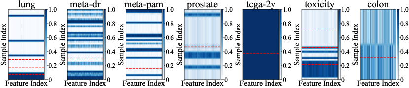
(a) Heatmaps of mask values from LLSPIN

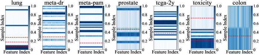
(b) Heatmaps of mask values from LSPIN

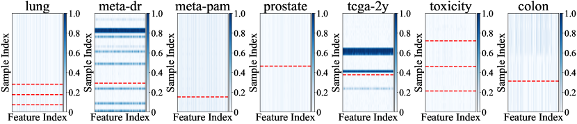
(c) Heatmaps of mask values from ProtoGate

Figure C.1: Comparison of the mask values on real-world datasets. We plot the heatmaps of predicted mask values ${\bm{s}}^{(i)}$ of test samples, where the x-axis refers to the indices of features, and the y-axis refers to the indices of samples. The samples are sorted according to their ground truth labels, and the red dash lines separate samples of different classes. Observing the heatmaps, we find that ProtoGate consistently learns more homogeneous feature patterns across samples compared to LSPIN/LLSPIN across various real-world datasets. Note that the different feature selection results across samples demonstrate that ProtoGate still preserves the ability to identify and leverage heterogeneous feature patterns for local feature selection.

Appendix D Ablation Impact of the Number of Nearest Neighbours $K$

In order to evaluate the behaviour of the prototype-based predictor, we conducted experiments using different numbers of nearest neighbours denoted as $K$. Considering the limited sample sizes of the datasets under investigation, we set the maximum number of nearest samples to $K=5$. All other experimental settings were kept consistent to ensure a fair comparison.

Table D.5 presents the results of the ablation experiments on the number of nearest neighbours, demonstrating that the optimal value of $K$ varies across different datasets. It is observed that using a small value of $K$ can make the predictions more sensitive to noise and outliers, resulting in lower accuracy. Notably, ProtoGate consistently achieves high accuracy across the range of $K\in\{3,4,5\}$. This finding supports the validity of the clustering assumption for the utilised real-world datasets, as ProtoGate exhibits stable and accurate performance.

Table D.5: Balanced accuracy for different numbers of neighbours in prototype-based classification, averaged over 25 runs. We bold the highest accuracy for each dataset. A small $K\in\{1,2\}$ can lead to sensitivity to noise, and the model performs stably with $K\in\{3,4,5\}$.

	lung	meta-dr	meta-pam	prostate	tcga-2y	toxicity	colon
$K=1$	87.53 $\pm$ 7.28	50.50 $\pm$ 6.21	73.02 $\pm$ 10.90	75.91 $\pm$ 10.21	57.46 $\pm$ 6.85	75.85 $\pm$ 7.02	70.40 $\pm$ 14.45
$K=2$	92.30 $\pm$ 7.28	56.06 $\pm$ 7.29	90.28 $\pm$ 6.01	86.93 $\pm$ 7.33	59.40 $\pm$ 6.24	88.81 $\pm$ 7.01	77.35 $\pm$ 13.46
$K=3$	93.44 $\pm$ 6.37	57.82 $\pm$ 8.93	95.96 $\pm$ 3.93	89.53 $\pm$ 5.64	61.18 $\pm$ 6.47	91.14 $\pm$ 5.19	81.10 $\pm$ 12.14
$K=4$	90.34 $\pm$ 7.01	60.43 $\pm$ 7.61	95.03 $\pm$ 4.77	88.85 $\pm$ 5.87	60.97 $\pm$ 5.60	91.10 $\pm$ 4.93	75.25 $\pm$ 13.34
$K=5$	91.12 $\pm$ 6.36	59.23 $\pm$ 6.88	95.83 $\pm$ 5.89	90.58 $\pm$ 5.64	60.84 $\pm$ 5.88	92.34 $\pm$ 5.67	77.50 $\pm$ 8.67

Appendix E Comparison of Training Duration

Figure E.2: Comparison of training duration on real-world datasets. TabNet is the fastest method, but its accuracy is substantially lower than other methods. ProtoGate has a shorter training duration than INVASE and similar computation efficiency as L2X.

References

- [1] Andreas D Baxevanis, Gary D Bader, and David S Wishart. Bioinformatics. John Wiley & Sons, 2020.
- [2] Arthur Lesk. Introduction to bioinformatics. Oxford university press, 2019.
- [3] Andrzej Polanski and Marek Kimmel. Bioinformatics. Springer Science & Business Media, 2007.
- [4] Arthur L Hsu, Sen-Lin Tang, and Saman K Halgamuge. An unsupervised hierarchical dynamic self-organizing approach to cancer class discovery and marker gene identification in microarray data. Bioinformatics, 19(16):2131–2140, 2003.
- [5] Junchen Yang, Ofir Lindenbaum, and Yuval Kluger. Locally sparse neural networks for tabular biomedical data. In International Conference on Machine Learning, pages 25123–25153. PMLR, 2022.
- [6] Yu Fan, Sanguo Zhang, and Shuangge Ma. Survival analysis with high-dimensional omics data using a threshold gradient descent regularization-based neural network approach. Genes, 13(9):1674, 2022.
- [7] Roman Levin, Valeriia Cherepanova, Avi Schwarzschild, Arpit Bansal, C Bayan Bruss, Tom Goldstein, Andrew Gordon Wilson, and Micah Goldblum. Transfer learning with deep tabular models. arXiv preprint arXiv:2206.15306, 2022.
- [8] Jinsung Yoon, James Jordon, and Mihaela van der Schaar. Invase: Instance-wise variable selection using neural networks. In International Conference on Learning Representations, 2018.
- [9] Bo Liu, Ying Wei, Yu Zhang, and Qiang Yang. Deep neural networks for high dimension, low sample size data. In IJCAI, pages 2287–2293, 2017.
- [10] Ravid Shwartz-Ziv and Amitai Armon. Tabular data: Deep learning is not all you need. Information Fusion, 81:84–90, 2022.
- [11] Polina Mamoshina, Armando Vieira, Evgeny Putin, and Alex Zhavoronkov. Applications of deep learning in biomedicine. Molecular pharmaceutics, 13(5):1445–1454, 2016.
- [12] Makoto Aoshima, Dan Shen, Haipeng Shen, Kazuyoshi Yata, Yi-Hui Zhou, and James S Marron. A survey of high dimension low sample size asymptotics. Australian & New Zealand journal of statistics, 60(1):4–19, 2018.
- [13] Andrei Margeloiu, Nikola Simidjievski, Pietro Lio, and Mateja Jamnik. Weight predictor network with feature selection for small sample tabular biomedical data. AAAI Conference on Artificial Intelligence, 2023.
- [14] Beatriz Remeseiro and Veronica Bolon-Canedo. A review of feature selection methods in medical applications. Computers in biology and medicine, 112:103375, 2019.
- [15] Sercan Ö Arik and Tomas Pfister. Tabnet: Attentive interpretable tabular learning. In Proceedings of the AAAI Conference on Artificial Intelligence, volume 35, pages 6679–6687, 2021.
- [16] Jianbo Chen, Le Song, Martin Wainwright, and Michael Jordan. Learning to explain: An information-theoretic perspective on model interpretation. In International Conference on Machine Learning, pages 883–892. PMLR, 2018.
- [17] Neil Jethani, Mukund Sudarshan, Yindalon Aphinyanaphongs, and Rajesh Ranganath. Have we learned to explain?: How interpretability methods can learn to encode predictions in their interpretations. In International Conference on Artificial Intelligence and Statistics, pages 1459–1467. PMLR, 2021.
- [18] Julius Adebayo, Justin Gilmer, Michael Muelly, Ian Goodfellow, Moritz Hardt, and Been Kim. Sanity checks for saliency maps. Advances in neural information processing systems, 31, 2018.
- [19] Sara Hooker, Dumitru Erhan, Pieter-Jan Kindermans, and Been Kim. A benchmark for interpretability methods in deep neural networks. Advances in neural information processing systems, 32, 2019.
- [20] Andreas Holzinger, Georg Langs, Helmut Denk, Kurt Zatloukal, and Heimo Müller. Causability and explainability of artificial intelligence in medicine. Wiley Interdisciplinary Reviews: Data Mining and Knowledge Discovery, 9(4):e1312, 2019.
- [21] Alex John London. Artificial intelligence and black-box medical decisions: accuracy versus explainability. Hastings Center Report, 49(1):15–21, 2019.
- [22] Julia Amann, Alessandro Blasimme, Effy Vayena, Dietmar Frey, Vince I Madai, and Precise4Q Consortium. Explainability for artificial intelligence in healthcare: a multidisciplinary perspective. BMC medical informatics and decision making, 20:1–9, 2020.
- [23] Sandeep Reddy. Explainability and artificial intelligence in medicine. The Lancet Digital Health, 4(4):e214–e215, 2022.
- [24] Erico Tjoa and Cuntai Guan. A survey on explainable artificial intelligence (xai): Toward medical xai. IEEE transactions on neural networks and learning systems, 32(11):4793–4813, 2020.
- [25] Olivier Chapelle, Bernhard Scholkopf, and Alexander Zien. Semi-supervised learning. 2006. Cambridge, Massachusettes: The MIT Press View Article, 2, 2006.
- [26] Janet L Kolodner. An introduction to case-based reasoning. Artificial intelligence review, 6(1):3–34, 1992.
- [27] Oscar Li, Hao Liu, Chaofan Chen, and Cynthia Rudin. Deep learning for case-based reasoning through prototypes: A neural network that explains its predictions. In Proceedings of the AAAI Conference on Artificial Intelligence, volume 32, 2018.
- [28] Isabelle Bichindaritz and Cindy Marling. Case-based reasoning in the health sciences: What’s next? Artificial intelligence in medicine, 36(2):127–135, 2006.
- [29] Isabelle Bichindaritz. Case-based reasoning in the health sciences: Why it matters for the health sciences and for cbr. In Advances in Case-Based Reasoning: 9th European Conference, ECCBR 2008, Trier, Germany, September 1-4, 2008. Proceedings 9, pages 1–17. Springer, 2008.
- [30] Yang Young Lu, C Yu Timothy, Giancarlo Bonora, and William Stafford Noble. Ace: Explaining cluster from an adversarial perspective. In International Conference on Machine Learning, pages 7156–7167. PMLR, 2021.
- [31] Aditya Grover, Eric Wang, Aaron Zweig, and Stefano Ermon. Stochastic optimization of sorting networks via continuous relaxations. arXiv preprint arXiv:1903.08850, 2019.
- [32] Robert Tibshirani. Regression shrinkage and selection via the lasso. Journal of the Royal Statistical Society: Series B (Methodological), 58(1):267–288, 1996.
- [33] Jean Feng and Noah Simon. Sparse-input neural networks for high-dimensional nonparametric regression and classification. arXiv preprint arXiv:1711.07592, 2017.
- [34] Makoto Yamada, Wittawat Jitkrittum, Leonid Sigal, Eric P Xing, and Masashi Sugiyama. High-dimensional feature selection by feature-wise kernelized lasso. Neural computation, 26(1):185–207, 2014.
- [35] Makoto Yamada, Jiliang Tang, Jose Lugo-Martinez, Ermin Hodzic, Raunak Shrestha, Avishek Saha, Hua Ouyang, Dawei Yin, Hiroshi Mamitsuka, Cenk Sahinalp, et al. Ultra high-dimensional nonlinear feature selection for big biological data. IEEE Transactions on Knowledge and Data Engineering, 30(7):1352–1365, 2018.
- [36] Héctor Climente-González, Chloé-Agathe Azencott, Samuel Kaski, and Makoto Yamada. Block hsic lasso: model-free biomarker detection for ultra-high dimensional data. Bioinformatics, 35(14):i427–i435, 2019.
- [37] Dinesh Singh, Héctor Climente-González, Mathis Petrovich, Eiryo Kawakami, and Makoto Yamada. Fsnet: Feature selection network on high-dimensional biological data. arXiv preprint arXiv:2001.08322, 2020.
- [38] Muhammed Fatih Balın, Abubakar Abid, and James Zou. Concrete autoencoders: Differentiable feature selection and reconstruction. In International conference on machine learning, pages 444–453. PMLR, 2019.
- [39] Ismael Lemhadri, Feng Ruan, and Rob Tibshirani. Lassonet: Neural networks with feature sparsity. In International Conference on Artificial Intelligence and Statistics, pages 10–18. PMLR, 2021.
- [40] Yutaro Yamada, Ofir Lindenbaum, Sahand Negahban, and Yuval Kluger. Feature selection using stochastic gates. In International Conference on Machine Learning, pages 10648–10659. PMLR, 2020.
- [41] Marco Tulio Ribeiro, Sameer Singh, and Carlos Guestrin. " why should i trust you?" explaining the predictions of any classifier. In Proceedings of the 22nd ACM SIGKDD international conference on knowledge discovery and data mining, pages 1135–1144, 2016.
- [42] Scott M Lundberg and Su-In Lee. A unified approach to interpreting model predictions. Advances in neural information processing systems, 30, 2017.
- [43] Avanti Shrikumar, Peyton Greenside, and Anshul Kundaje. Learning important features through propagating activation differences. In International conference on machine learning, pages 3145–3153. PMLR, 2017.
- [44] Karen Simonyan, Andrea Vedaldi, and Andrew Zisserman. Deep inside convolutional networks: Visualising image classification models and saliency maps. arXiv preprint arXiv:1312.6034, 2013.
- [45] Scott M Lundberg, Gabriel G Erion, and Su-In Lee. Consistent individualized feature attribution for tree ensembles. arXiv preprint arXiv:1802.03888, 2018.
- [46] Sebastian Bach, Alexander Binder, Grégoire Montavon, Frederick Klauschen, Klaus-Robert Müller, and Wojciech Samek. On pixel-wise explanations for non-linear classifier decisions by layer-wise relevance propagation. PloS one, 10(7):e0130140, 2015.
- [47] Yuya Yoshikawa and Tomoharu Iwata. Neural generators of sparse local linear models for achieving both accuracy and interpretability. Information Fusion, 81:116–128, 2022.
- [48] Ronald J Williams. Simple statistical gradient-following algorithms for connectionist reinforcement learning. Reinforcement learning, pages 5–32, 1992.
- [49] George Tucker, Andriy Mnih, Chris J Maddison, John Lawson, and Jascha Sohl-Dickstein. Rebar: Low-variance, unbiased gradient estimates for discrete latent variable models. Advances in Neural Information Processing Systems, 30, 2017.
- [50] Makoto Yamada, Takeuchi Koh, Tomoharu Iwata, John Shawe-Taylor, and Samuel Kaski. Localized lasso for high-dimensional regression. In Artificial Intelligence and Statistics, pages 325–333. PMLR, 2017.
- [51] Wojciech Samek, Alexander Binder, Grégoire Montavon, Sebastian Lapuschkin, and Klaus-Robert Müller. Evaluating the visualization of what a deep neural network has learned. IEEE transactions on neural networks and learning systems, 28(11):2660–2673, 2016.
- [52] Guolin Ke, Qi Meng, Thomas Finley, Taifeng Wang, Wei Chen, Weidong Ma, Qiwei Ye, and Tie-Yan Liu. Lightgbm: A highly efficient gradient boosting decision tree. Advances in neural information processing systems, 30, 2017.
- [53] Leo Breiman. Random forests. Machine learning, 45:5–32, 2001.
- [54] Evelyn Fix. Discriminatory analysis: nonparametric discrimination, consistency properties, volume 1. USAF school of Aviation Medicine, 1985.
- [55] Arindam Bhattacharjee, William G Richards, Jane Staunton, Cheng Li, Stefano Monti, Priya Vasa, Christine Ladd, Javad Beheshti, Raphael Bueno, Michael Gillette, et al. Classification of human lung carcinomas by mrna expression profiling reveals distinct adenocarcinoma subclasses. Proceedings of the National Academy of Sciences, 98(24):13790–13795, 2001.
- [56] Dinesh Singh, Phillip G Febbo, Kenneth Ross, Donald G Jackson, Judith Manola, Christine Ladd, Pablo Tamayo, Andrew A Renshaw, Anthony V D’Amico, Jerome P Richie, et al. Gene expression correlates of clinical prostate cancer behavior. Cancer cell, 1(2):203–209, 2002.
- [57] Gagan Bajwa, Ralph J DeBerardinis, Baomei Shao, Brian Hall, J David Farrar, and Michelle A Gill. Cutting edge: Critical role of glycolysis in human plasmacytoid dendritic cell antiviral responses. The Journal of Immunology, 196(5):2004–2009, 2016.
- [58] Chris Ding and Hanchuan Peng. Minimum redundancy feature selection from microarray gene expression data. Journal of bioinformatics and computational biology, 3(02):185–205, 2005.
- [59] Christina Curtis, Sohrab P Shah, Suet-Feung Chin, Gulisa Turashvili, Oscar M Rueda, Mark J Dunning, Doug Speed, Andy G Lynch, Shamith Samarajiwa, Yinyin Yuan, et al. The genomic and transcriptomic architecture of 2,000 breast tumours reveals novel subgroups. Nature, 486(7403):346–352, 2012.
- [60] Arthur Liberzon, Chet Birger, Helga Thorvaldsdóttir, Mahmoud Ghandi, Jill P Mesirov, and Pablo Tamayo. The molecular signatures database hallmark gene set collection. Cell systems, 1(6):417–425, 2015.
- [61] Katarzyna Tomczak, Patrycja Czerwińska, and Maciej Wiznerowicz. The cancer genome atlas (tcga): an immeasurable source of knowledge. Contemporary oncology, 19(1A):A68, 2015.
- [62] William Falcon and The PyTorch Lightning team. PyTorch Lightning, March 2019.
- [63] Adam Paszke, Sam Gross, Francisco Massa, Adam Lerer, James Bradbury, Gregory Chanan, Trevor Killeen, Zeming Lin, Natalia Gimelshein, Luca Antiga, et al. Pytorch: An imperative style, high-performance deep learning library. Advances in neural information processing systems, 32, 2019.
- [64] Fabian Pedregosa, Gaël Varoquaux, Alexandre Gramfort, Vincent Michel, Bertrand Thirion, Olivier Grisel, Mathieu Blondel, Peter Prettenhofer, Ron Weiss, Vincent Dubourg, et al. Scikit-learn: Machine learning in python. the Journal of machine Learning research, 12:2825–2830, 2011.
- [65] Takuya Akiba, Shotaro Sano, Toshihiko Yanase, Takeru Ohta, and Masanori Koyama. Optuna: A next-generation hyperparameter optimization framework. In Proceedings of the 25th ACM SIGKDD International Conference on Knowledge Discovery and Data Mining, 2019.