SmartPUR: An Autonomous PUR Transmission Solution for Mobile C-IoT Devices

Abstract

Cellular Internet-of-things (C-IoT) user equipments (UEs) typically transmit frequent but small amounts of uplink data to the base station. Undergoing a traditional random access procedure (RAP) to transmit a small but frequent data presents a considerable overhead. As an antidote, preconfigured uplink resources (PURs) are typically used in newer UEs, where the devices are allocated uplink resources beforehand to transmit on without following the RAP. A prerequisite for transmitting on PURs is that the UEs must use a valid timing advance (TA) so that they do not interfere with transmissions of other nodes in adjacent resources. One solution to this end is to validate the previously held TA by the UE to ensure that it is still valid. While this validation is trivial for stationary UEs, mobile UEs often encounter conditions where the previous TA is no longer valid and a new one is to be requested by falling back on legacy RAP. This limits the applicability of PURs in mobile UEs. To counter this drawback and ensure a near-universal adoption of transmitting on PURs, we propose new machine learning aided solutions for validation and prediction of TA for UEs of any type of mobility. We conduct comprehensive simulation evaluations across different types of communication environments to demonstrate that our proposed solutions provide up to a $98.7$% accuracy in predicting the TA.

I Introduction

Billions of devices that can gather and transmit data, including wearables, smart meters, intelligent vehicles, and next-generation transportation systems, to name a few, are being connected to the Internet [1]. With a large growth in such interconnected devices, i.e., the Internet-of-things (IoT), there is a constant need for innovation in Low-Power Wide-Area (LPWA) cellular technologies to ensure massive connectivity and enhanced energy efficiency for IoT devices [2, 3]. The 3rd Generation Partnership Project (3GPP) introduced the long-term evolution for machine type communication (LTE-M) and narrowband IoT (NB-IoT) specifications to specifically address the requirements of LPWA cellular networks [4, 5, 6, 7], which have been regularly enhanced to meet the needs of growing IoT networks [8, 9].

IoT user equipements (UEs) are typically battery powered and supplied as a single charge version [10, 11, 12]. Hence, to ensure longer battery life, cellular IoT (C-IoT) UEs generally remain in idle state, employing discontinuous reception (DRX), extended discontinuous reception (eDRX), and/or power saving mode (PSM) [13]. Such an operation is suitable for IoT applications since the IoT traffic typically consists of short and infrequency blocks of data. However, a C-IoT UE that is in an idle mode must establish connection and enter a connected active mode to transmit data to the base station (BS) [14]. This connection establishment procedure consumes an extended period of time. While this may be acceptable for mobile broadband applications that have extended lengths of data payload to transmit, this overhead is magnified in the case of C-IoT applications that significantly reduces the battery life of these devices.

Connection establishment in C-IoT networks involves a random access procedure (RAP) during which time the network UEs contend with each other to obtain resources for bidirectional communication. A standard 4-step contention-based RAP involves at least four message exchanges between the UE and BS before a connection is established [7, 15]. To reduce this overhead in C-IoT networks, the use of early data transmission (EDT) was considered to piggyback short uplink data together with RAP messages [16]. EDT reduced the network latency by up to three seconds and extended the battery life of C-IoT UEs by up to three years [16]. The gains are further increased with the use of preconfigured uplink resources (PURs), where the C-IoT UEs are allotted resources beforehand, which they can then use for uplink transmission without undergoing any RAP message exchange [17]. One of the conditions for using PURs is that the UE must apply a valid timing advance for its transmission, that is, the UE must advance its signal transmission by an amount dictated by the propagation delay between the UE and the BS. Failure to do so potentially causes interference between transmissions of UEs using adjacent resources. Therefore, every UE must first validate its TA before attempting a PUR transmission. The TA held by the UE is obtained either during PUR configuration or via a PUR response following a successful PUR transmission.

I-A Drawbacks with the State-of-the-art Designs

TA validation is a trivial task for stationary UEs, since the propagation delay between the UE and the BS remains constant. However, supporting mobile C-IoT UEs requires designing TA validation strategies to minimize inter-UE interference. The use of mobile IoT devices in smart cities, vehicular communication links, and post-emergency networks [18, 19, 20], among others, motivate the challenge of addressing TA validation for mobile devices in a C-IoT network. TA validation essentially involves determining whether a mobile UE has moved beyond a permissible movement (PM) that is dependent on the length of cyclic prefix used in the orthogonal frequency division multiplexed (OFDM) transmission. Current-day 3GPP specifications allow UEs to validate TAs in a centralized approach using the PUR time alignment timer (PUR-TAT) configured centrally by the BS and/or a distributed approach where UEs validate the TA using the measured reference signal received power (RSRP) [14]. The latter is a dynamic technique that does not require assistance from the BS and is motivated by the correlation between the measured RSRP and the UE-BS separation. As the UE moves away from the BS, the measured RSRP reduces due to increased path-loss and the TA increases due to a larger propagation delay, and vice versa. Thus, the state-of-the-art RSRP-based TA validation method [14, Sec. 5.3.3] uses a threshold-based approach, where the difference in the measured RSRP (in logarithmic scale) between the two UE locations is compared against a positive and a negative threshold to determine whether the UE has moved beyond the PM.

We identify three issues with the state-of-the-art method. First, the technique is highly dependent on the fixed thresholds that are set based on path loss models [21, 22, 23]. This idealized assumption is not always reliable and data-driven methods are preferable in such scenarios, as also identified in our prior work [21]. We build on this idea and provide detailed investigation and methodologies for TA validation for expanding the use of PURs. Following our proposal in [21], data-driven methods for obtaining an indication of TA have also been investigated in the context of expediting random access [24], along the lines of machine learning (ML) - based timing estimation proposed for various facets of communication systems [25, 26, 27]. A second issue with legacy threshold-based TA validation is that the computation of thresholds and error margins are optimized for several redundant initial UE positions. For example, when the UE is near the cell-edge, further movement away from the BS sends the UE out of the cell, in which case, it can no longer use PURs irrespective of its TA. Recognizing such conditions is critical in improving error margins while designing threshold computations. Finally, we identify a fundamental drawback with the idea of TA validation. When a UE determines a TA to be invalid, legacy approach requires the UE to fallback on either EDT or 4-step RAP to obtain a new TA. Therefore, mobile UEs that often move beyond the PM rarely use PURs. On the other hand, a C-IoT UE can always use PURs if, in place of validating the TA, it instead directly predicted the TA at any given location.

I-B Contributions

To counter the drawbacks we identified with the state-of-the-art TA validation technique [14, Sec. 5.3.3], we propose SmartPUR. SmartPUR consists of two component choices, a smart TA validator (sTAV) and a smart TA predictor (sTAP). sTAV is an enhanced TA validator that validates the previously held TA and extrapolates it as the current TA to be used for PUR transmission. When the latest TA held by the UE is deemed to be invalid, it mandates UEs to fallback on legacy TA acquisition methods as specified in [14, Sec. 5.3.3]. sTAP, on the other hand, estimates the TA at any given UE location using its previous TA and the difference in RSRP, such that the UE can always use PURs. A C-IoT UE could either use one of sTAV or sTAP. Although the use of sTAP is more attractive as it offers more than simply validating an existing TA, sTAV may be applicable in scenarios where the network is incompatible with UEs proactively using an estimated TA. For instance, a 5G BS may not allow UEs to use any TA other than the one it configures the UE with so that UEs do not intentionally or unintentionally cause network congestion due to the use of inaccurate TAs.

The contributions of our work can be listed as follows.

• We propose an enhanced threshold-based TA validation procedure as part of SmartPUR that improves the performance of the state-of-the-art RSRP-based TA validation for PUR transmission. Our modified solution identifies when the UE is at the cell-boundary or close to the BS and recognizes that there is no further movement away or toward the BS, respectively, that can invalidate the TA while still remaining in the same cell. The new positive and negative validation thresholds that we develop using this prior knowledge enhances the detection rates and reduces false alarms in validating the TA.

• We design an ML-aided solution for TA validation that requires less signaling overhead compared to the threshold-based approach. We demonstrate the robustness of our solution to operate in an environment-agnostic fashion and show that our method matches the detection rate and significantly reduces false alarms for TA validation when compared to the threshold-based approach.

• We advance the adoption of PURs in C-IoT networks by designing a TA prediction method. We provide a closed-form expression for TA estimate computation based on the difference in RSRP and the previous TA. Furthermore, we use supervised ML regression to design a predictor that can estimate the TA at any given location of the UE and for any movement that the UE has undergone. We then quantize the estimated floating-point TA for use during the PUR transmission.

• We conduct a comprehensive evaluation campaign to investigate the performance of our proposed solutions. We perform end-to-end link-level simulations under diverse communication environments and UE movements to evaluate the validation and prediction accuracy for using SmartPUR.

I-C Outline

The rest of this paper is organized as follows. We describe the system model used in our work in Section II. We propose our novel sTAV and sTAP solutions in Section III and Section IV, respectively. In Section V, we present the performance evaluation results of our proposed solutions. We reflect on our proposed methods to identify the application scenarios and potential implementation limitations of our methods in Section VI. We conclude our paper in Section VII.

Notation: Throughout the paper, the $\log$ operator represents logarithm to base $10$.

II System Model

Figure 1: An example illustration of two C-IoT UEs and their corresponding PM regions for using PURs with their previously held TAs. (Objects in the image are not to scale.)

We consider an LTE-M/NB-IoT system, such as the one shown in Fig. 1, where a BS serves C-IoT UEs within a cell. We consider a cell radius between $1.5$ km, which is characteristic of an urban setting, to $5$ km, that may be seen in a more rural environment. Our choice of the lower end of cell size is based on TA validation for small cells (e.g., indoor distributed systems) being trivial due to the limited intra-cell mobility of UEs. On the other hand, we choose the higher end of the cell size based on typical values of cell radius in real-world deployments.

C-IoT traffic is typically sporadic and uplink heavy in nature, with data packet inter-arrival times commonly ranging between few seconds to a day [28, Annex. E], [29, Annex. A]. To save battery between transmissions, C-IoT UEs enter a sleep state using DRX. Accordingly, the UE enters an idle DRX (IDRX) mode after the completion of message exchange with the BS and a subsequent wait period. Upon request for data transfer either by the BS on IDRX pages (mobile terminated data) or by the application for uplink data (mobile originated data), the UE enters an active connected mode, which requires an extended duration of time to complete the RAP prior to entering the active connected mode [16]. When the UE has a small amount of data to transmit, the uplink data can be piggybacked on one of the RAP messages for faster completion using EDT to achieve a battery life extension of up to three years. By using PURs, power consumption can be reduced further by up to $50\%$ when compared to EDT [17].

Figure 2: A UE attempting PUR transmissions from two different locations at $\ell_{1}$ and $\ell_{2}$.

We consider a C-IoT network that uses PURs, where the BS configures UEs with PURs as requested either by the network or the UEs themselves [17]. The UEs are allowed to use the PURs so long as they remain in the same cell. Additionally, the PURs may also be configured with a PUR TAT, upon whose expiration, the TA held by the UE is no longer considered to be valid. Alternatively or additionally, the network may set the PUR TAT to a large value and allow the UEs to determine the validity of the TA independently by monitoring the RSRP. Static UEs, e.g., cellular-connectivity-enabled smart meters, can always use the TA that is provided during PUR configuration. However, TAs change with movement for mobile UEs such as terrestrial vehicles, mobile robots, aerial vehicles, and wearables [30]. As a result, the TAs must be validated before a PUR transmission. We call the region within which the last available TA held by the UE is considered to be valid as the PM region, as shown in Fig. 1. As long as the UE is within this PM region when it attempts the next PUR transmission, it can continue to use the TA it received from the BS at the end of the previous PUR transmission. The width of this area is dependent on the extent to which an incorrect TA can be tolerated at the BS. This is in turn dependent on the length of the cyclic prefix used by the OFDM PUR transmission. Using LTE-M specifications with a sub-carrier spacing (SCS) of $15$ kHz, the cyclic prefix spans $4.7~{}\mu$s, which corresponds to a maximum permissible movement of $\Delta d_{\text{per}}=702$ m. Notice that this PM does not dictate a general movement of the UE, but instead a movement that causes the UE-BS separation to increase more than $702$ m from its previous separation. For instance, if the UE moves along a circle with the BS as the center of the circle, irrespective of the actual distance traversed by the UE, the change in the UE-BS separation would be zero. When the UE uses an invalid TA, i.e., when the UE uses its TA when its movement violates the condition,

$$\Delta d\leq\Delta d_{\text{per}},$$ (1)

where $\Delta d$ indicates the difference in the UE-BS distances between the current and the previous UE locations, its PUR transmission may interfere with UEs using adjacent resources. Consider an example of UE movement as shown in Fig. 2. At two different time instances (for example, at two PUR transmission instances), the UE is located at $\ell_{1}$ and $\ell_{2}$ that are at distances of $d_{1}$ and $d_{2}$ from the BS. In this scenario,

$$\Delta d=|d_{2}-d_{1}|,$$ (2)

and not the distance between $\ell_{2}$ and $\ell_{1}$.

TAs are provided and updated by the BS in quantized amounts. The quantized version of the TA, $\tau_{\text{q}}$, can be represented as

$$\tau_{\text{q}}=\left\lfloor\frac{d}{2c\tau_{\text{step}}}\right\rfloor,$$ (3)

where $d$ is the distance between the UE and the BS, $\tau_{\text{step}}$ is the quantization step, which is equal to $0.52~{}\mu$s for LTE-M with an SCS of $15$ kHz, and $c$ is the speed of light. Accordingly, we represent the deviation in $\tau_{\text{q}}$ corresponding to $\Delta d_{\text{per}}$ as $\Delta\tau_{\text{q},{\text{per}}}$.

III TA Validation

Legacy TA validation can be performed in two ways. The first is a centralized approach, where the BS provides the UE with a PUR-TAT. The UE is then allowed to use PURs, i.e., determine that the previously held TA by the UE is valid, when the PUR-TAT is running [14]. When the PUR-TAT expires, the UE no longer considers the TA to be valid. The BS determines the value of PUR-TAT based the UE mobility and the periodicity of the PURs. A primary concern with such a centralized approach is that the movement of the UE is not always deterministic or uniform. Therefore, the BS often conservatively provides a lower value of PUR-TAT to ensure that the UE does not use an invalid TA. A better alternative to this method is a distributed approach, which allows the UEs to determine the TA validity based on the correlation between the TA and a measured power metric, such as RSRP. In the following, we focus on such an RSRP-based TA validation to improve the accuracy of detecting the TA validity.

RSRP is computed as the linear average of the power contributions of resource elements (REs) that carry cell-specific reference signals (CRSs), measured over a certain bandwidth. The measurement bandwidth and the number of REs used to determine RSRP, however, is left to UE implementation [31]. The locations of the REs carrying the CRSs are determined using the physical ID of the camped cell which is obtained when the UE is synchronized using the primary synchronization signal (PSS) and secondary synchronization signal (SSS) [32]. The measured RSRP, $P_{\text{RSRP}}$, can be represented as

$$P_{\text{RSRP}}=\frac{P_{\text{TX}}}{\alpha(d_{i})},$$ (4)

where $P_{\text{TX}}$ is the CRS transmit power used by the BS and $\alpha(d_{i})$ is the net power loss for a mobile UE that is located at $\ell_{i}$, which is at a distance $d_{i}$ from the BS. Across different types of environments, (4) can be represented in its general form as [33]

$$P_{{\text{RSRP}},i}=\frac{P_{\text{TX}}}{\beta_{i}d_{i}^{k_{i}}},$$ (5)

where $k_{i}$ is the path-loss exponent and $\beta_{i}$ is the scaling coefficient accounting for system losses at the $i$th location of the UE. Consider a UE movement from an initial location $\ell_{i-1}$ to a new one at $\ell_{i}$, as shown in Fig. 2 (for $i=2$). The difference in RSRP in logarithmic scale is

$$\Delta P_{{\text{RSRP}},i,\text{dB}}=\log\left(\frac{\beta_{i}d_{i}^{k_{i}}}{\beta_{i-1}d_{i-1}^{k_{i-1}}}\right).$$ (6)

Assuming that the path-loss characteristics are the same at the two UE locations, i.e., with $\beta_{i-1}=\beta_{i}$ and $k_{i-1}=k_{i}=k$, (6) can be simplified as

$$\Delta P_{{\text{RSRP}},i,\text{dB}}=k\log\left(\frac{d_{i}}{d_{i-1}}\right).$$ (7)

Since $P_{\text{RSRP}}$ does not vary linearly with $d$, the observed $\Delta P_{{\text{RSRP}},\text{dB}}$ is not the same for a UE movement toward and away from the BS. Therefore, for a UE at the $i$th location, the threshold-based TA validation compares the measured $\Delta P_{{\text{RSRP}},\text{dB}}$ against a positive and a negative threshold, $\Delta P_{\max,\text{pos}}$ and $\Delta P_{\max,\text{neg}}$, respectively, which are computed as [21]

$$\begin{split}\Delta P_{\max,i,\text{pos}}&=k\log\left(1+\frac{\Delta d_{\text{per}}}{d_{i-1}}\right)-\epsilon_{\text{pos}}\\ \Delta P_{\max,i,\text{neg}}&=k\log\left(1-\frac{\Delta d_{\text{per}}}{d_{i-1}}\right)+\epsilon_{\text{neg}},\end{split}$$ (8)

where $\epsilon_{\text{pos}}$ and $\epsilon_{\text{neg}}$ are error margins used to account for measurement errors and channel variations. The error margins can be dynamically adjusted by the BS to achieve a desired level of validation accuracy, e.g., by sacrificing false alarms for improving detection rates.

III-A Threshold-based sTAV

We incorporate (7) and (8) as the starting point for building the threshold-based sTAV. Since $\Delta P_{\max,i,\text{pos}}$ and $\Delta P_{\max,i,\text{neg}}$ must always be positive and negative, respectively, and RSRP monotonically decreases with distance, the limits on $\epsilon_{\text{pos}}$ and $\epsilon_{\text{neg}}$ can be computed at the cell boundary as

$$\begin{split}0&<\epsilon_{{\text{pos}}}<k\log\left(1+\frac{\Delta d_{\text{per}}}{r_{\text{cell}}}\right)\\ 0&<\epsilon_{{\text{neg}}}<-k\log\left(1-\frac{\Delta d_{\text{per}}}{r_{\text{cell}}}\right),\end{split}$$ (9)

where $r_{\text{cell}}$ is the approximate cell size. However, when the UE is close to the cell-edge, i.e., when $r_{\text{cell}}-\Delta d_{\text{per}}<d_{i-1}\leq r_{\text{cell}}$, there is no movement away from the BS that will render the TA to be invalid. The UE either moves such that $\Delta d\leq\Delta d_{\text{per}}$, in which case its TA is still valid, or moves such that $\Delta d>\Delta d_{\text{per}}$ and exits the cell and can thus no longer use PURs. Similarly, when the UE is in close proximity to the BS, i.e., when $d_{i-1}\leq\Delta d_{\text{per}}$, there is no movement toward the BS that will render the TA to be invalid. Exploiting these two factors, sTAV using threshold-based TA validation uses a modified detection approach as outlined in Algorithm 1. This also allows us to use larger error margins which are bounded by

$$\begin{split}0&<\epsilon_{{\text{pos}}}<-k\log\left(1-\frac{\Delta d_{\text{per}}}{r_{\text{cell}}}\right)\\ 0&<\epsilon_{{\text{neg}}}<-k\log\left(1-\frac{\Delta d_{\text{per}}}{r_{\text{cell}}-\Delta d_{\text{per}}}\right).\end{split}$$ (10)

Note that for Algorithm 1, sTAV uses $d_{i-1}$ that is obtained using (3) with $\tau_{\text{q},i-1}$, where $\tau_{\text{q},i-1}$ is the actual TA value provided by the BS when the UE completes a successful PUR transmission while being located at $l_{i-1}$. We show in Section V that sTAV in Algorithm 1 with (10) matches the performance of legacy TA validation for detecting invalid TA conditions and significantly improves performance of identifying valid ones.

Algorithm 1 The proposed threshold-based sTAV.

Compute $\Delta P_{\max,i,\text{pos}}$ and $\Delta P_{\max,i,\text{neg}}$ using (8)

while PUR data to transmit in idle mode do:

Detect CRS and measure $\Delta P_{{\text{RSRP}},i,\text{dB}}$

if $d_{i-1}<\Delta d_{{\text{per}}}$ then

     TA valid if: $\Delta P_{{\text{RSRP}},i,\text{dB}}<\Delta P_{\max,i,\text{pos}}$

else

     if $d_{i-1}>r_{{\text{cell}}}-\Delta d_{\text{per}}$ then

         TA valid if: $\Delta P_{{\text{RSRP}},i,\text{dB}}>\Delta P_{\max,i,\text{neg}}$

     else

         TA valid if: $\Delta P_{\max,i,\text{neg}}\!<\!\Delta P_{{\text{RSRP}},i,\text{dB}}\!<\!\Delta P_{\max,i,\text{pos}}$

     end if

end if

III-B ML-aided sTAV

Although the threshold-based sTAV improves the performance of TA validation when compared to the state-of-the-art [14, Sec. 5.3.3], it still suffers from measurement inaccuracies due to the impact of noise at low signal-to-noise ratio (SNR) conditions, fading effects of the channel, and deviation of the practical environment behavior from the path-loss model used in computing the thresholds. To address this model deficit, we explore data-driven approaches using ML for TA validation. Our target is to develop a robust sTAV scheme, where a machine that is trained with synthetic data generated using one or more path-loss models can operate under any typical cellular channel and noise environment. Training the machine with synthetic data provides us the freedom to use as many data samples as required for training to achieve the desired performance.

III-B1 Formulating the Problem

We formulate the problem as a supervised binary classification task, where a classifier determines if the previously held TA is valid or not based on the difference in RSRP, i.e.,

$$\hat{\tau}_{\text{q},i} ={\texttt{sTAV}}(\tau_{\text{q},i-1},\Delta P_{{\text{RSRP}},i,\text{dB}})$$

$$=\begin{cases}\tau_{\text{q},i-1},&\text{if valid}\\ \infty,&\text{if invalid},\end{cases}$$ (11)

where $\hat{\tau}_{\text{q},i}$ is the output TA of sTAV at the $i$th PUR transmission instance. A result of $\hat{\tau}_{\text{q},i}=\infty$ indicates to the UE that the previous TA is invalid. In such cases, the UE must fallback to other downward compatible network access methods, e.g., EDT, 4-step RAP, or 2-step RAP, for data transmission and TA acquisition.

We characterize the performance of sTAV in terms of the true negative rate (TNR), $p_{\text{TN}}$, and the true positive rate (TPR), $p_{\text{TP}}$, of the classifier. We define true negatives as the cases where sTAV indicates that $\hat{\tau}_{\text{q},i}=\infty$, when the TA is actually invalid. Therefore, the false positive rate (FPR), $p_{\text{FP}}$ can be written as

$$p_{\text{FP}}=1-p_{\text{TN}},$$ (12)

indicating the rate of false positives where the TA is determined to be valid by sTAV when the TA is in fact invalid. Along the same lines, we define true positives as conditions where sTAV indicates the previously held TA to be valid when the TA is valid, and consequently, the false negative rate (FNR), $p_{\text{FN}}$, can be defined as

$$p_{\text{FN}}=1-p_{\text{TP}}.$$ (13)

We summarize the conditions and outcomes of sTAV in Table I.

TABLE I: Conditions and Outcomes of sTAV

Condition	Actual TA	Predicted TA
True Positive (TP)	Valid	Valid
True Negative (TN)	Invalid	Invalid
False Positive (FP)	Invalid	Valid
False Negative (FN)	Valid	Invalid

III-B2 Training the Machine

We consider the use of support vector machine (SVM) and adaptive boosting (AdaBoost) algorithms for sTAV [34], as both these algorithms have been shown in the past to provide accurate performance in similar classification tasks [35]. We train our machine using synthetic data of $\Delta P_{{\text{RSRP}},i}$ and $\tau_{\text{q},i-1}$ generated using different path loss models. We train our machines by introducing a higher penalty for false positives. We realize this by weighting false positives higher in our loss function minimization to target a $p_{\text{TN}}\geq 90\%$. Recall that false positives result in scenarios where the UE uses an invalid TA for PUR transmission, which causes increased interference with neighboring resource transmissions. This renders the use of PURs to be a net negative to the overall system functioning when compared to not using PURs. However, a false negative leads only to a conservative self-deterrence, whose operation is equivalent to a non-PUR transmission.

We randomize the UE movement such that its location in a two-dimensional space is drawn from a uniformly distributed random variable between a distance $0$ to $d_{\max}$ from the BS. This ensures that the generated $\ell_{i}$s are uncorrelated and our machine is not trained for any set trajectory of motion. By randomizing the locations of the UE, the UE velocity, UE movement trajectory, and PUR periodicity do not impact our emulation of UE positions during PUR transmissions. However, the UE velocity does impact the RSRP measurement within the UE due to varying Doppler shift effects on UEs with different velocities. We emulate various types of UEs, such as pedestrian UEs, slow moving vehicles, and UEs mounted on high-speed automobiles, by using a range of different UE velocities. Recall that the computation of $\Delta P_{{\text{RSRP}},i}$ is up to UE implementation as per the existing standard [31]. This gives us the ability to devise efficient standard-compliant RSRP computation techniques. To this end, we explore non-coherent combining techniques to improve the reliability of the measured $\Delta P_{{\text{RSRP}},i}$.

We use the CRS transmitted periodically by the BS to determine RSRP. Using a larger number of CRS sub-frames (SFs) for combining assists in reducing the impact on non-idealities, such as Doppler effects and noise, on the measured RSRP. However, larger the numbers of CRS SFs used, higher is the power consumption in the UE and longer is the time-to-measure of RSRP. The number of CRS SFs required to achieve a satisfactory performance (i.e., for our trained machine to achieve our target $p_{\text{TN}}$ and $p_{\text{TP}}$) depends on the UE velocity and the operating SNR. We evaluated the accuracy of the measured RSRP for different UE velocities between stationary to $120$ km/hr and varying operating SNRs for UEs that are close to the BS to up to $5$ km away from the BS in urban macro and rural environments. We observed that using $4$ CRS SFs that are each picked once every $10$ ms (or $10$ SFs) apart for combining provides a suitable trade-off between measurement accuracy and computation complexity/time. Therefore, we use this setting throughout training and testing the performance of our method. We show in Section V that this setting allows us to meet our target performance.

III-B3 Tuning the Machine

One of the goals of using ML for sTAV is to ensure that SmartPUR is applicable across a variety of path-loss environments irrespective of what was used during training. To verify this, we evaluate the robustness of our method by training our machine using one path-loss model and test its performance across a range of others. This also provides an insight into our design of training the machine using synthetic data and deploying it in the real-world. To better adapt to practical model deviation, we also scale the computed $\Delta P_{{\text{RSRP}},i}$ before inputting it into our classifier. Consider a machine that is trained using a path-loss model with $k_{\text{train}}$ and implemented in an environment with a path loss exponent $k_{\text{system}}$. We scale the RSRP difference that is input to the machine as

$$\Delta P_{{\text{RSRP}},i,\text{dB}}\leftarrow\Delta P_{{\text{RSRP}},i,\text{dB}}\frac{k_{\text{train}}}{k_{\text{system}}}.$$ (14)

This scaling ensures that $\Delta P_{{\text{RSRP}},i,\text{dB}}\propto k_{\text{train}}\log\left(\frac{d_{i}}{d_{i-1}}\right)$ as seen by the machine during training. We observed that this scaling operation provides a noticeable improvement in the classification accuracy when operating under environments that were different from the ones used during training. This scaling operation, however, requires the signaling of an estimate of $k_{\text{system}}$ to the UE by the BS that can be done either during PUR configuration and/or updated at any time during operation. Note that this scaling only assists in countering the mismatch of path-loss models. Even with an accurate path-loss model estimated by the BS and signaled to the UE, our designed method must still be robust in countering the RSRP measurement inaccuracies introduced due to fading effects and due to the impact of noise at low operating SNRs.

III-B4 Choice of sTAV

We evaluate the performance of sTAV in Section V for both modes of operation, i.e., using the threshold- and ML-based approaches. We leave the choice of sTAV mode to UE implementation depending on the performance accuracy and implementation complexity trade-off that is desired. For example, a low-complexity NB-IoT UE may choose to use the threshold-based sTAV, whereas achieving superior classification performance may be prioritized for a coverage enhanced LTE-M device.

IV TA Prediction

TA validation, either using sTAV shown in Section III or the state-of-the-art method [14, Sec. 5.3.3], is efficient in enabling UEs to determine conditions when they can use an old TA for a new PUR transmission. This technique is suitable for UEs in relatively smaller cells. As the cell size increases, the probability of UEs moving beyond PM increases. In such cases, the UE must fall-back on legacy RAPs like EDT or 4-step RAP to acquire a new TA from the BS. This limits the use of PURs in such cases. To counter this, we propose an alternative method that ensures that UEs can always use PURs. In lieu of validating TA, we propose the use of sTAP to instead predict the TA at any given UE location so that the UE can use the predicted TA for PUR transmission.

TA prediction using sTAP in place of TA validation also eliminates the restriction of PUR usage to movement within the PM. It allows system-wide implementation irrespective of the transmission parameters such as the OFDM sub-carrier spacing or environment characteristics like the cell-size. A system implementation of this method is straightforward to achieve by letting the network set PUR TAT to $\infty$ and allowing UEs to use sTAP for TA determination.

Using sTAP, a UE begins by predicting a TA for any given UE location where the UE has a PUR data to transmit using current and historical RSRP values and a previous TA. We describe the prediction techniques in detail in Section IV-A and Section IV-B. The UE then uses the predicted TA to perform a PUR transmission. Upon successful reception of the PUR packet, the BS provides the UE with the actual TA of the transmission. The UE then updates its currently held TA with the one received from the BS, which it then uses for the subsequent TA prediction. The UE thereby always uses an actual TA from previous iterations for predicting a current TA. Therefore, any error in predicting a TA does not carryover or compound over predictions, since the UE always receives an accurate TA value from the BS after every PUR transmission.

Using sTAP reduces the average fallback rate for PUR transmissions, which is the probability of UEs falling back on legacy methods (e.g., EDT or RAP-based transmission) for TA acquisition. Falling back on legacy (i.e., non-PUR) approaches is costly for a UE due to the increased power consumption associated with acquiring a new TA, e.g., with an EDT or a RAP-based transmission, when compared to a PUR transmission [17].

We categorize the UE fallback on to legacy methods into the following two types:

1. Proactive fallback: In case of proactive fallback, the UE falls back to a legacy channel access procedure based on determining that the TA held by the UE is inaccurate. With the use of sTAV, the UE proactively falls back when the sTAV indicates $\hat{\tau}_{\text{q},i}=\infty$.

2. Reactive fallback: The UE falls back in a reactive manner when the UE uses an invalid TA, which leads to an unsuccessful PUR transmission. Upon learning of such an unsuccessful transmission (e.g., either by the BS indicating a failed detection or by the UE conducting repeated unsuccessful PUR transmission attempts), the UE falls back to legacy methods for channel access.

We denote the proactive and reactive fallback rates for sTAV and sTAP as $p_{\text{f,pro},{\texttt{sTAV}}}$, $p_{\text{f,re},{\texttt{sTAV}}}$, $p_{\text{f,pro},{\texttt{sTAP}}}$, and $p_{\text{f,re},{\texttt{sTAP}}}$, respectively. We then define the overall fallback rates for the sTAV and sTAP methods as

$$p_{\text{f},{\texttt{sTAV}}} =p_{\text{f,pro},{\texttt{sTAV}}}+p_{\text{f,re},{\texttt{sTAV}}}$$ (15)

$$p_{\text{f},{\texttt{sTAP}}} =p_{\text{f,pro},{\texttt{sTAP}}}+p_{\text{f,re},{\texttt{sTAP}}},$$ (16)

respectively.

Next, we characterize the fallback rates based on the performance of sTAV and sTAP. Using sTAV, the two events where the UE proactively falls back are when the UE has moved beyond the PM with sTAV correctly indicating an invalid TA, and when the UE has moved within the PM with sTAV incorrectly indicating an invalid TA. Therefore, we can represent the proactive fallback rate of sTAV as

$$p_{\text{f,pro},{\texttt{sTAV}}}=p_{\Delta d>\Delta d_{\text{per}}}p_{\text{TN}}+(1-p_{\Delta d>\Delta d_{\text{per}}})p_{\text{FN}},$$ (17)

where $p_{\Delta d>\Delta d_{\text{per}}}$ is the probability that the UE moves beyond the PM for using the previously held TA but remains within the same serving cell. The condition where the UE reactively falls back is when the UE incorrectly uses an invalid TA and learns about the TA validity after one or more unsuccessful PUR transmission attempts. Therefore,

$$p_{\text{f,re},{\texttt{sTAV}}}=p_{\Delta d>\Delta d_{\text{per}}}p_{\text{FP}}.$$ (18)

Finally, using (12), (15), (17), and (18), we determine

$$p_{\text{f},{\texttt{sTAV}}}=p_{\Delta d>\Delta d_{\text{per}}}+(1-p_{\Delta d>\Delta d_{\text{per}}})p_{\text{FN}}.$$ (19)

On the other hand, using sTAP, we eliminate the cases of the UE proactively falling back to legacy method since the UE always performs a PUR transmission using the predicted TA. Therefore, the only fall back cases are when the UE inaccurately predicts the TA and reactively falls back. Therefore,

$$p_{\text{f},{\texttt{sTAP}}}=p_{\text{f,re},{\texttt{sTAP}}}=1-\eta,$$ (20)

where $\eta$ is the prediction accuracy of sTAP. Recall that the cyclic prefix provides a buffer for using an inaccurate TA that is quantified in terms of the PM. Therefore, the TA prediction accuracy must only be equivalent to a UE movement within the PM. That is, if the predicted TA corresponds to an estimated UE-BS distance of $\tilde{d}_{i}$ and the actual UE-BS separation is $d_{i}$, the TA prediction is accurate if $\Delta d_{i}=|d_{i}-\tilde{d}_{i}|\leq\Delta d_{\text{per}}$. Therefore,

$$\eta=\frac{1}{2N_{\text{obs}}}\sum\limits_{i=1}^{N_{\text{obs}}}\left(1+\mathrm{sgn}(\Delta d_{\text{per}}-\Delta d_{i})\right),$$ (21)

where $\mathrm{sgn}(x)$ is a modified sign function which we define as

$$\mathrm{sgn}(x)\triangleq\begin{cases}+1,&\text{if }x=0\\ \frac{|x|}{x},&\text{otherwise }\end{cases}$$ (22)

and $N_{\text{obs}}$ is the number of observations over which the accuracy is computed. When $\Delta d_{i}>\Delta d_{\text{per}}$ PUR transmission fails due to the use of an inaccurate transmission. However, this condition is equivalent to the false positives in TA validation where the validator wrongly indicates an invalid TA to be valid. Therefore, similar to the TNR in sTAV, we set our target $\eta\geq 0.9$ for sTAP.

IV-A Equation-based sTAP

Similar to the threshold-based sTAV in Section III-A, we build an sTAP method using pre-defined and well-developed path-loss models. Estimating the TA after any UE movement can be drawn directly from the analysis in Section III. Using (3) and (7), we can compute the TA at the $i$th UE location as

$$\hat{\tau}_{\text{q},i}=\left\lfloor 10^{\frac{\Delta P_{{\text{RSRP}},i,\text{dB}}}{k}}\frac{d_{i-1}}{2c\tau_{\text{step}}}\right\rfloor,$$ (23)

where $\hat{\tau}_{\text{q},i}$ is the TA predicted by sTAP for the $i$th PUR transmission (similar to the output TA in (11)). The value of $d_{i-1}$ used in (23) is computed as

$$d_{i-1}=2c\tau_{\text{step}}{\tau}_{\text{q},i-1},$$ (24)

where ${\tau}_{\text{q},i-1}$ is the actual TA value provided by the BS after a successful PUR transmission at the $(i-1)$th instance (and not the predicted $\hat{\tau}_{\text{q},i-1}$).

This method introduces little computational complexity over the threshold-based sTAV to directly estimate the TA. The signaling requirements associated with the use of this method are also the same as those for the threshold-based method, i.e., the path-loss exponent is conveyed to the UE by the BS either during PUR configuration or any time during operation such as along with the PUR response. However, due to the nature of the estimation that relies significantly on the accuracy of the path-loss model and the accurate computation of $\Delta P_{{\text{RSRP}},i,\text{dB}}$ within the UE, it suffers from the same drawbacks as the threshold-based sTAV. To address these challenges, we investigate the use of data driven methods in the ML-aided sTAP.

IV-B ML-aided sTAP

We design our ML-aided sTAP along similar lines as that of the ML-aided sTAV. We formulate the problem as a supervised ML regression task where a regressor uses one or more prior values of TA and RSRP and the current RSRP measured by the UE to estimate the TA at the new UE location, i.e.,

$$\hat{\tau}_{\text{q},i}={\texttt{sTAP}}(\tau_{\text{q},i-1},P_{{\text{RSRP}},i,\text{dB}}).$$ (25)

Similar to the procedure shown in Section III, we also scale the values of $P_{{\text{RSRP}},i,\text{dB}}$ as in (14) before inputing the data into our regressors to account for possible environment mismatches.

We use the least squares boosting (L2Boost) algorithm to train the regressor. L2Boost consolidates multiple weak learners into a strong learner by applying weak learners to weighted versions of the data with higher weights allocated to samples suffering greater inaccuracies in previous rounds [34, Ch. 16]. Additionally, it is also robust to over-fitting, which is particularly beneficial to our case of unrestricted training samples that we generate synthetically using established path-loss models.

The use of ML techniques also allows us to design prediction schemes that use more than one prior TA and RSRP information for predicting the current TA. Such a multi-input regression uses historical raw data of the measured RSRP and predictions to estimate the new TA, i.e.,

$$\hat{\tau}_{\text{q},i}={\texttt{sTAP}}({\tau}_{\text{q},i-k},P_{{\text{RSRP}},i-k+1,\text{dB}}),\;\;k=\{1,2,...\mathcal{K}\}$$ (26)

where $k$ is the index of the number of historical values used for prediction, and $\mathcal{K}$ is the total number of historical values used.

V Results

We present the simulation results of the performance of our proposed sTAV and sTAP techniques to evaluate the accuracy of our validation and prediction, respectively.

V-A Simulation Settings

TABLE II: Fixed Simulation Settings

Parameter	Value
Carrier Frequency	$0.9$ GHz
System Bandwidth	$1.4$ MHz
Transmit Power	$46$ dBm
Receiver Noise Figure	$9$ dB
Thermal Noise Floor	$-174$ dBm/Hz
No. of Transmitter Antennas	$1$
No. of Receiver Antennas	$1$

We use the LTE-M specifications for our simulations. We perform link-level simulations by emulating the BS and UE transceivers in their entirety at the physical layer. We list the fixed settings of our simulations in Table II. Note that the signal of interest is the CRS, and hence we consider a unidirectional transmission link (i.e., only the downlink) with the BS and the UE as the transmitter and receiver, respectively.

We use the system model described in Section II. We use a variable cell size between typical urban cell radius of $1.5$ km and a larger macro cell with radius of up to $5$ km. We use three different path loss models for large-scale fading, the urban micro (UMi), urban macro (UMa), and rural macro (RMa), which we obtain from the 5G channel models presented in TR 38.901 [36]. To avoid repetitiveness, we do not regurgitate the path loss expressions, which can be found in [36, Sec. 7.4]. We use the path-loss exponent of the testing model as an input to sTAV and sTAP when testing the robustness of our methods to perform under unseen conditions. Note that in a practical implementation, this corresponds to a best-guess estimate of the path-loss exponent made by the BS and signaled dynamically to the UE.

We also use the tapped delay line (TDL) channel models to emulate the small-scale fading effects [36, Sec. 7.7]. Since a mobile UE experiences different types of environment depending on its position in the cell, we use a varying line-of-sight probability computed as in [36, Sec. 7.4.2]. Based on this, we pick the TDL model between TDL-A to TDL-E accordingly. Further, we simulate different types of communication environments using three different average delay spreads, the short, normal, and long spreads from [36, Sec. 7.7.3], for scaling the delays of the power delay profiles of our considered channel models. Additionally, to capture a wide range of application scenarios from stationary sensors to use in high-speed automobiles, we introduce a random UE speed of up to $120$ km/hr, which introduces Doppler effects that impact the measurement of $P_{\text{RSRP}}$ as described in Section III-B2.

V-B sTAV

We use TPR and TNR, i.e., sensitivity and specificity, respectively, of sTAV as its key performance indicators. An ideal classifier attempts to maximize both the contradictory metrics of sensitivity and specificity. However, for a practical design it is critical to consider the importance of each of these to develop strategies to sacrifice one to improve the other. A high specificity is critical in ensuring that the FPR is low and as a result, fewer instances of an invalid TA are used for PUR transmission. This reduces the inter-UE interference caused due to the use of an invalid TA. On the other hand, a higher FNR is less costly as it only causes redundant fallback on non-PUR schemes but not interference with UEs using adjacent resources. Therefore, we target a specificity of $p_{\text{TN}}>90\%$, which is consistent with targets proposed in prior arts [22, 23], and a sensitivity of $p_{\text{TP}}>50\%$ such that PURs are used more often than not under valid TA conditions. To this end, we apply a mis-classification cost for false positives that is five times higher than that for false negatives during training.

V-B1 Threshold-based sTAV

(a)

(b)

Figure 3: The (a) specificity and (b) sensitivity of legacy and sTAV methods for TA validation.

We present our first result of specificity and sensitivity of the threshold-based sTAV and legacy TA validation in Fig. 3. We notice that while sTAV matches the sensitivity of legacy methods, the use of smarter error margins allows the specificity to be increased over the legacy validation method. For example, with an $r_{\text{cell}}=5$ km, legacy TA validation performs so poorly that around $6$ out of $10$ PUR transmission opportunities are wasted due to inaccurate validation results. On the other hand, the threshold-based sTAV  exceeds the target TPR of $50\%$ in all evaluation conditions.

V-B2 ML-aided sTAV

(a)

(b)

Figure 4: The (a) specificity and (b) sensitivity of sTAV methods for TA validation.

It is clear from Fig. 3 that a threshold-based sTAV provides the target specificity. However, our evaluation results of the ML-aided sTAV shows the improvement in sensitivity achievable using our ML-aided approach. Fig. 4 shows that ML-aided sTAV using both SVM and AdaBoost match the specificity of the threshold-based sTAV and provides noticeable improvement in sensitivity. However, under large macro cells at $r_{\text{cell}}=5$ km, the AdaBoost based sTAV falls behind the threshold- and the SVM-based sTAV marginally, while still providing higher than a $50\%$ PUR usage rate.

(a)

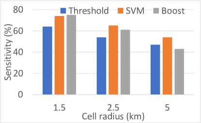
(b)

Figure 5: The (a) specificity and (b) sensitivity of sTAV methods for TA validation with cross path-loss model training and testing.

Fig. 5 presents the same comparison as in Fig. 4 for a more realistic evaluation setting, where the machines for the ML-aided sTAV are trained and tested under different channel models. This captures practical conditions, where real-world channels need not necessarily fit any of the channel models that may be used during training. As an example, we used the urban macro path-loss model for training, and the urban micro path-loss model for the sub-2.5 km cell radius and the rural macro path-loss model for the 5 km cell radius case when testing. The positive results in Fig. 4, i.e., a $>90\%$ specificity and $>50\%$ sensitivity (except for the AdaBoost based sTAV) demonstrates that our proposed method can be used in an offsite training based deployment. An offsite training based deployment consists of a setting where the machines are trained offline using synthetic computer generated data, for example, using a best emblematic channel model of the potential environment, and deployed in the real-world to function using practically extracted measurements within a UE. Together with eliminating the restriction on the number of training samples, such a training regimen also minimizes the startup time that may be required by a learn-as-you-go approach that incurs inaccurate performance initially until acquiring sufficient data to improve its performance.

V-C sTAP

(a)

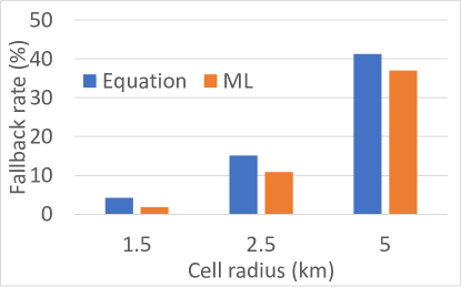
(b)

Figure 6: The fallback rate for an equation based sTAP method and an ML aided sTAP method with machines that were trained and tested on (a) the same path-loss model and (b) on different path-loss models.

As explained in Section IV, sTAP provides the ability for UEs to proactively estimate the TA value for PUR transmission so that PURs can be used at all required instances. We quantify the performance of our TA prediction solution using the fallback rate as defined in (20). Fig. 6(a) and 6(b) show the fallback rates for our proposed sTAP solution with a uni-model and a cross-model training and testing approaches, respectively. We followed the same cross-model training and testing strategy as described in Section V-B. Our first takeaway from the results is that the performance of our solution is robust across channel conditions drawn from path-loss models unseen during training. Secondly, the fallback rate from using our method is negligible when operating under typical urban cell-sizes with radius under a mile, especially with the ML-aided sTAP. Finally, we notice that the fallback rates increase with the radius of the cell with large cells encountering more instances where UEs fallback to RAP-based uplink transmissions for small data packets.

TABLE III: Fallback rates for sTAV and sTAP

$d_{\text{cell}}$ (km)	$p_{\text{FP},{\texttt{sTAV}}}$	$p_{\Delta d>\Delta d_{\text{per}}}$	$p_{\text{f},{\texttt{sTAV}}}$	$p_{\text{f},{\texttt{sTAP}}}$
$1.5$	$29\%$	$25\%$	$47\%$	$1.9\%$
$1.5$	$29\%$	$50\%$	$65\%$	$1.9\%$
$1.5$	$29\%$	$75\%$	$82\%$	$1.9\%$
$2.5$	$35\%$	$25\%$	$51\%$	$11\%$
$2.5$	$35\%$	$50\%$	$68\%$	$11\%$
$2.5$	$35\%$	$75\%$	$84\%$	$11\%$
$5$	$46\%$	$25\%$	$60\%$	$37\%$
$5$	$46\%$	$50\%$	$73\%$	$37\%$
$5$	$46\%$	$75\%$	$87\%$	$37\%$

To provide context for the fallback rate numbers, we contrast our sTAP values to the fallback probability observed with using a TA validation approach. The best performing TA validation method is the SVM-based sTAV as seen in Section V-B. We use the FPR of SVM-based sTAV in (19) to compute the fallback probability of the validation method. Observe from (19) that the fallback rate for TA validation further depends on $p_{\Delta d>\Delta d_{\text{per}}}$. Greater the value of $p_{\Delta d>\Delta d_{\text{per}}}$ for a UE, higher is the fallback rate since TA validation attempts to invalidate and prohibit UEs from using PURs when $\Delta d>\Delta d_{\text{per}}$. On the other hand, our sTAP solution proactively predicts the TA such that a UE can always use PURs.

We present the average fallback rates in Table III. We tabulate the results for three different values of $p_{\Delta d>\Delta d_{\text{per}}}=\{25\%,50\%,75\%\}$ to account for different possible UE movements and PUR transmission intervals. For instance, a highly mobile UE with a large interval between successive PUR occasions may have a higher $p_{\Delta d>\Delta d_{\text{per}}}$ than a UE that moves slower with more frequent PUR transmissions. We observe that using sTAP significantly reduces the fallback rates and improves the usability of PURs. While we target an ideal zero fallback rate, which our ML-aided sTAP comes close to in relatively small cells, any reduction in the fallback rate over the TA validation approach improves the applicability of PUR. The worst-case fallback probabilities of sTAP, which is at $d_{\text{cell}}=5$ km, still cuts the fallback rates of sTAV by more than half in highly mobile UEs. Since using PURs has been shown to reduce UE power consumption by about $50\%$ [17], slashing the fallback rates by over half significantly improves the battery life of C-IoT UEs.

VI Discussion

Before concluding the paper, in this section, we reflect on our proposed solutions by discussing their applicability in practical systems and providing guidelines for potential implementation designs.

VI-A Standardization

3GPP has adopted the threshold- and RSRP-based TA validation in the LTE-M and NB-IoT specifications [14]. Since the computation of RSRP is up to UE implementation, our threshold-based sTAV method can be readily adopted into present-day C-IoT UEs. Further, the configuration of TA validation conditions for using PURs is optional in the LTE-M and NB-IoT specifications [14]. Therefore, network providers can choose to enable any of our sTAV and/or sTAP methods on compatible UEs without any specification changes to the LTE-M and/or NB-IoT standards to counter the impact of model deficits on PUR transmissions.

VI-B Interpretation of SmartPUR

Throughout our paper, we present our smart TA validation and prediction solutions considering the usage of PUR. However, our methods are equally applicable to (pre)-configured grant based periodic small data uplink transmission, e.g., configured grant small data transmission (CG-SDT) in the 5G/new radio (NR) standards, which also includes an RSRP-based TA validation procedure [37]. Similarly, our methods are applicable in all application scenarios that use a TA estimate that can be predicted using current and historical values of received signal power values beyond for use in small data transmission, e.g., for a 2-step RAP with improved TA estimation.

VI-C Implementation Designs

The offline training based deployment approach discussed in Section V-B is one of several approaches of implementing our proposed solution. Training the machines can also be performed in the real-world at the BS-end to ensure no increase in complexity at the C-IoT UEs. The RSRP and TA values can be collected by the BS from the several UEs in a given environment (e.g., a cell or a sector of the cell) to train a machine. The BS can exploit the reciprocal nature of frequency division duplex channels and use uplink reference signals such as the sounding reference signal to obtain the path-loss characteristics of the channel, similar to the architecture presented in [24].

VII Conclusion

We presented SmartPUR, which is an autonomous PUR transmission solution for mobile C-IoT devices. Our solution includes two options for validating and/or predicting the TA at any given PUR transmission instance. Our smart TA validator leverages historical path-loss measurements and trained ML models to intelligently predict whether a previously held TA is valid for PUR transmission at a considered instance. We expanded on this design to present a smart TA predictor that exploits the same historical path-loss data to predict a TA at any PUR transmission opportunity using ML-aided regression techniques. Our comprehensive simulation evaluation across a variety of channel conditions demonstrated the effectiveness of both of our design approaches in the real-world. Measurement collection and prototype development to bring our proposed solutions to hardware implementation guides our future work.

References

- [1] L. Xu, R. Collier, and G. M. O’Hare, “A survey of clustering techniques in WSNs and consideration of the challenges of applying such to 5G IoT scenarios,” IEEE Internet of Things J., vol. 4, no. 5, pp. 1229–1249, 2017.
- [2] L. Chettri and R. Bera, “A comprehensive survey on internet of things (IoT) toward 5G wireless systems,” IEEE Internet of Things J., vol. 7, no. 1, pp. 16–32, 2019.
- [3] G. A. Akpakwu, B. J. Silva, G. P. Hancke, and A. M. Abu-Mahfouz, “A survey on 5G networks for the Internet of Things: Communication technologies and challenges,” IEEE Access, vol. 6, pp. 3619–3647, 2017.
- [4] A. D. Zayas and P. Merino, “The 3GPP NB-IoT system architecture for the Internet of Things,” in IEEE Int. Conf. on Commun. Workshops (ICC Workshops), 2017, pp. 277–282.
- [5] A. Hoglund, X. Lin, O. Liberg, A. Behravan, E. A. Yavuz, M. Van Der Zee, Y. Sui, T. Tirronen, A. Ratilainen, and D. Eriksson, “Overview of 3GPP release 14 enhanced NB-IoT,” IEEE network, vol. 31, no. 6, pp. 16–22, 2017.
- [6] M. B. Hassan, E. S. Ali, R. A. Mokhtar, R. A. Saeed, and B. S. Chaudhari, “NB-IoT: concepts, applications, and deployment challenges,” in LPWAN Technologies for IoT and M2M Applications. Elsevier, 2020, pp. 119–144.
- [7] H. Althumali and M. Othman, “A survey of random access control techniques for machine-to-machine communications in LTE/LTE-A networks,” IEEE Access, vol. 6, pp. 74 961–74 983, 2018.
- [8] C. Kuhlins, B. Rathonyi, A. Zaidi, and M. Hogan, “Cellular networks for massive IoT,” Jan., 2020, Ericsson Whitepaper.
- [9] GSMA, “Mobile IoT in the 5G future: NB-IoT and LTE-M in the context of 5G,” Apr., 2018, GSMA Whitepaper.
- [10] G. Callebaut, G. Leenders, J. Van Mulders, G. Ottoy, L. De Strycker, and L. Van der Perre, “The art of designing remote IoT devices—technologies and strategies for a long battery life,” Sensors, vol. 21, no. 3, 2021.
- [11] R. Ratasuk, B. Vejlgaard, N. Mangalvedhe, and A. Ghosh, “NB-IoT system for M2M communication,” in IEEE Wireless Commun. Netw. Conf. (WCNC), 2016, pp. 1–5.
- [12] X. Lu, I. H. Kim, A. Xhafa, J. Zhou, and K. Tsai, “Reaching 10-years of battery life for industrial IoT wireless sensor networks,” in IEEE Symposium on VLSI Circuits, 2017, pp. C66–C67.
- [13] Rohde and Schwarz, “Power saving methods for LTE-M and NB-IoT devices,” Jun., 2019, R&S Whitepaper.
- [14] TS 36.331 V16.7.0 , “Evolved universal terrestrial radio access (E-UTRA) radio resource control (RRC) protocol specification (Release 16),” 3rd Generation Partnership Project (3GPP), Tech. Spec., Dec., 2021.
- [15] W. Li, Q. Du, L. Liu, P. Ren, Y. Wang, and L. Sun, “Dynamic allocation of RACH resource for clustered M2M communications in LTE networks,” in IEEE Int. Conf. Identification, Information, and Knowledge in the Internet of Things (IIKI), 2015, pp. 140–145.
- [16] A. Hoglund, D. P. Van, T. Tirronen, O. Liberg, Y. Sui, and E. A. Yavuz, “3GPP release 15 early data transmission,” IEEE Commun. Standards Mag., vol. 2, no. 2, pp. 90–96, 2018.
- [17] A. Hoglund, G. Medina-Acosta, S. N. K. Veedu, O. Liberg, T. Tirronen, E. A. Yavuz, and J. Bergman, “3GPP release-16 preconfigured uplink resources for LTE-M and NB-IoT,” IEEE Commun. Standards Mag., vol. 4, no. 2, pp. 50–56, 2020.
- [18] W. Ayoub, A. E. Samhat, F. Nouvel, M. Mroue, and J.-C. Prévotet, “Internet of mobile things: Overview of LoraWAN, dash7, and NB-IoT in LPWANs standards and supported mobility,” IEEE Commun. Surveys & Tuts., vol. 21, no. 2, pp. 1561–1581, 2018.
- [19] N. A. Surobhi and A. Jamalipour, “An IoT-based middleware for mobility management in post-emergency networks,” in International Conf. on Telecommun.(ICT), 2014, pp. 283–287.
- [20] A. Zanella, N. Bui, A. Castellani, L. Vangelista, and M. Zorzi, “Internet of things for smart cities,” Internet of Things J., vol. 1, no. 1, pp. 22–32, 2014.
- [21] G. Vos, A. A. N. Abdelnasser, and L. Lampe, “Method and apparatus for time advance validation using reference signal received power,” United States Patent Application 20200260397, Aug., 2020.
- [22] Sierra Wireless, “R4-1905499: LTE-M PUR RSRP TA validation design considerations,” 3GPP TSG RAN WG4 #91, Tech. Doc., May 2019.
- [23] ——, “R4-1905500: NB-IoT PUR NRSRP TA validation design considerations,” 3GPP TSG RAN WG4 #91, Tech. Doc., May 2019.
- [24] J. Kim, G. Lee, S. Kim, T. Taleb, S. Choi, and S. Bahk, “Two-step random access for 5G system: Latest trends and challenges,” IEEE Network, vol. 35, no. 1, pp. 273–279, 2021.
- [25] J. Schmitz, C. von Lengerke, N. Airee, A. Behboodi, and R. Mathar, “A deep learning wireless transceiver with fully learned modulation and synchronization,” in IEEE International Conference on Communications Workshops (ICC Workshops), 2019, pp. 1–6.
- [26] S. Ali, W. Saad, N. Rajatheva, K. Chang, D. Steinbach, B. Sliwa, C. Wietfeld, K. Mei, H. Shiri, H.-J. Zepernick et al., “6G white paper on machine learning in wireless communication networks,” arXiv preprint arXiv:2004.13875, 2020.
- [27] H. Wu, Z. Sun, and X. Zhou, “Deep learning-based frame and timing synchronization for end-to-end communications,” in Journal of Physics: Conference Series, vol. 1169, no. 1. IOP Publishing, 2019.
- [28] TR 45.820, “Cellular system support for ultra-low complexity and low throughput Internet of Things (CIoT),” 3rd Generation Partnership Project (3GPP), Tech. Rep., Nov. 2015.
- [29] TR 36.888, “Study on provision of low-cost Machine-Type Communications (MTC) User Equipments (UEs) based on LTE,” 3rd Generation Partnership Project (3GPP), Tech. Rep., Jun. 2013.
- [30] L. E. Talavera, M. Endler, I. Vasconcelos, R. Vasconcelos, M. Cunha, and F. J. d. S. e Silva, “The mobile hub concept: Enabling applications for the internet of mobile things,” in IEEE PERCOM Workshops, 2015, pp. 123–128.
- [31] TS 36.214 V16.1.0 , “Evolved universal terrestrial radio access (E-UTRA): Physical layer measurements (Release 16),” 3rd Generation Partnership Project (3GPP), Tech. Spec., Jun., 2020.
- [32] TS 36.211 V16.1.0 , “Evolved universal terrestrial radio access (E-UTRA): Physical layer measurements (Release 16),” 3rd Generation Partnership Project (3GPP), Tech. Spec., Jan., 2021.
- [33] TR 36.814, “Evolved Universal Terrestrial Radio Access (E-UTRA): Further advancements for E-UTRA physical layer aspects,” 3rd Generation Partnership Project (3GPP), Tech. Rep., Mar. 2017.
- [34] K. P. Murphy, Machine learning: a probabilistic perspective. MIT press, 2012.
- [35] C. Jiang, H. Zhang, Y. Ren, Z. Han, K. Chen, and L. Hanzo, “Machine learning paradigms for next-generation wireless networks,” IEEE Wireless Communications, vol. 24, no. 2, pp. 98–105, 2017.
- [36] TR 38.901, “Study on channel model for frequencies from 0.5 to 100 GHz,” 3rd Generation Partnership Project (3GPP), Tech. Rep., Jan. 2020.
- [37] A. Khlass and D. Laselva, “Efficient handling of small data transmission for RRC inactive UEs in 5G networks,” in IEEE Vehicular Technology Conference (VTC2021-Spring), 2021, pp. 1–7.