Twice Hidden String Order and Competing Phases in the Spin-1/2 Kitaev-Gamma Ladder

Abstract

Finding the Kitaev spin liquid in candidate materials involves understanding the entire phase diagram, including other allowed interactions. One of these interactions, called the Gamma ($\Gamma$) interaction, causes magnetic frustration and its interplay with the Kitaev ($K$) interaction is crucial to comprehend Kitaev materials. Due to the complexity of the combined K$\Gamma$ model, quasi-one dimensional models have been investigated. While several disordered phases are found in the 2-leg ladder, the nature of the phases are yet to be determined. Here we focus on the disordered phase near the antiferromagnetic $\Gamma$ limit (denoted by A$\Gamma$ phase) next to the ferromagnetic Kitaev phase. We report a distinct non-local string order parameter characterizing the A$\Gamma$ phase, different from the string order parameter in the Kitaev phase. This string order parameter becomes evident only after two unitary transformation, referred to as a twice hidden string order parameter. The related entanglement spectrum, edge states, magnetic field responses, and the symmetry protecting the phase are presented, and its relevance to the two-dimensional Kitaev materials is discussed. Two newly identified disordered phases in the phase diagram of K$\Gamma$ ladder is also reported.

Introduction

Over the course of investigating spin $S$=1/2 two-dimensional (2D) honeycomb Kitaev materials [1, 2, 3, 4, 5], candidates of long-sought quantum spin liquids, an additional bond-dependent spin exchange term named Gamma ($\Gamma$) interaction [6] was found along with the bond-dependent Kitaev ($K$) interaction [7, 8]. Unlike the standard Heisenberg interaction, both the Kitaev and the $\Gamma$ interactions are highly nontrivial and extremely frustrated. While the same sign of $K$ and $\Gamma$ cancels the frustration leading to magnetically ordered phases, the regions with different signs of these interactions are highly frustrated.[5] Since these two interactions are known to dominate over other symmetry-allowed interactions in the emerging candidate material $\alpha$-RuCl₃, the combined Kitaev-Gamma (K$\Gamma$) model has attracted considerable attention in the theoretical community and it is widely accepted [9, 10, 11] that a realistic description of $\alpha$-RuCl₃ should be sought in the regime with antiferromagnetic (AFM) Gamma ($\Gamma\mathord{>}$0) and ferromagnetic (FM) Kitaev ($K\mathord{<}$0) interactions. Understanding the phases that arise in this frustrated regime of the 2D honeycomb K$\Gamma$-model is therefore of crucial importance.

This particular region of the K$\Gamma$-model has been extensively studied by a range of numerical methods [5]. Despite detailed studies, the nature of the phase next to the FM Kitaev spin liquid arising due to AFM $\Gamma$ interaction remains controversial. Most studies have found that it is in a disordered phase [12, 13, 14, 15, 16, 17, 18, 19], denoted by K$\Gamma$SL for K$\Gamma$ spin liquid, or nematic paramagnets, but functional renormalization approaches found magnetically ordered phases [20] while variational Monte Carlo calculations [21] observed a narrow disordered phase next to the FM Kitaev spin liquid with most of the antiferromagnetic $\Gamma$ region dominated by a zig-zag ordered phase.

Motivated by such discrepancy, another approach to investigate the 2D limit of the K$\Gamma$ model was taken by starting from low-dimensional models with the hope of furthering the understanding of the honeycomb model by determining the phases of $n$-leg (brick-wall) models. Despite the obvious challenge in connecting the two limits, it is reasonable to expect that potential spin liquid phases arising in the honeycomb model should correspond to regions where the $n$-leg models display disordered phases. Such an approach was employed earlier for the pure Kitaev model [22]. Disordered phases in the anisotropic Kitaev 1-leg chain were found, and they were characterized by non-local string order parameters (SOPs)[22]. It has also been shown that the isotropic Kitaev 2-leg ladder model exhibits a disordered phase, characterized by an unconventional SOP different from that of the anisotropic chain Kitaev phase [23].

The one-dimensional (1D) chain and ladder version of the K$\Gamma$ model were investigated numerically with very high precision, as the reduced dimensionality allows accessing bigger system sizes [24, 25, 26, 27, 28]. In the 1D chain model, it was found that the pure Gamma model belongs to a Luttinger liquid phase governed by the gapless hidden SU(2) Heisenberg chain, a fact revealed after a 6-site transformation, i.e, a duality mapping [29, 24]. A study of the same K$\Gamma$ model on a quasi 1D ladder using DMRG and iDMRG techniques[18, 30] found a magnetically disordered phase, possessing a small gap near the AFM pure Gamma limit. This phase surrounding the pure AFM Gamma point next to the FM Kitaev phase (denoted by F$K$) was referred to as the A$\Gamma$ phase. Even though the A$\Gamma$ phase in the ladder occurs in the same part of the phase diagram as the proposed $K\Gamma$SL in the 2D limit, a distinct name was introduced, as it is yet to be determined how the A$\Gamma$ phase is connected to the 2D limit $K\Gamma$SL.

While it is clear that there is no magnetic order in this phase, the precise nature of the A$\Gamma$ phase has not yet been settled due to its complex nature. The presence of a gap indicates that the A$\Gamma$-phase is likely a symmetry protected topological (SPT) phase [31, 32, 33]. If so, it is of importance to identify a corresponding SOP, edge states, and the symmetry that protects this phase, which are characteristic of the SPT, and to determine how this phase respond to an external magnetic field. If strong evidence for a non-trivial SPT nature of the A$\Gamma$ phase can be established, it would establish a next step to the proposed $K\Gamma$SL in the 2D limit. In the following sections, we will systematically examine these inquiries and provide comprehensive responses. To perform a thorough analysis, we start by reviewing the full phase diagram prior to focusing on the nature of the A$\Gamma$ phase. As shown below, we also report two other disordered phases.

Results

Model

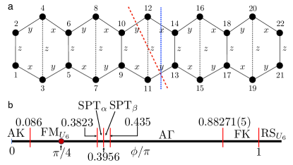
Figure 1: The K$\Gamma$ ladder and corresponding phase diagram. a A strip of the K$\Gamma$ honeycomb lattice corresponding to a two-leg K$\Gamma$ ladder with alternating $x$ and $y$ bonds along the leg and $z$-bond between the chains, with the numbering of the sites used throughout the paper. The dotted $z$-bonds arise from imposing periodic boundary conditions in the direction perpendicular to the ladder. However, all $z$-bonds are taken to have equal strength. The dashed red line indicates the partition used for $\rho_{B}$ while the dashed blue line indicates the partition used for $\rho_{A}$. b Schematic phase diagram of the K$\Gamma$ ladder, Eq. (1), for $\Gamma\mathord{>}$0.

The K$\Gamma$ Hamiltonian is given by

$$H_{K\Gamma}=\sum_{\langle i,j\rangle_{\gamma\in(x,y,z)}}KS_{i}^{\gamma}S_{j}^{\gamma}+\Gamma\left(S^{\alpha}_{i}S^{\beta}_{j}+S^{\beta}_{i}S^{\alpha}_{j}\right)$$ (1)

where $(\alpha,\beta)$ takes on the values $(y,z)/(x,z)/(x,y)$ for $\gamma=x/y/z$, and $\langle i,j\rangle$ refers to the nearest neighbor sites. An alternative representation of the honeycomb lattice is as a brick-wall lattice [22], and its two-leg limit with periodic boundary conditions is simply a ladder shown in Fig. 1a. The dotted bonds indicate Kitaev $z$-bonds arising from periodic boundary conditions, and we shall always take such bonds to be identical to the regular (solid) $z$-bonds, in which case the honeycomb strip can be viewed as a regular rectangular ladder.

We parameterize the model by taking

$$K=\cos\phi,\ \ \ \mathrm{and}\ \ \ \ \Gamma\mathord{=}\sin\phi,$$ (2)

and interpolate between the Kitaev and $\Gamma$ interactions by varying $\phi$. Our main interest is in the region with $\phi/\pi\in[0,\pi]$ where $\Gamma\mathord{>}$0 and the Kitaev term, $K$, changes from AFM to FM at $\phi$=$\pi$/2, as this region is relevant to most two-dimensional (2D) Kitaev candidate materials. The total number of sites in the ladder (including both legs) is denoted by $N$.

Phase Diagram

A full phase diagram is shown in Fig. 1b. It is obtained by various quantities presented in the next subsection. Moving from $\phi\mathord{=}0$ to $\pi$, the AFM Kitaev phase (denoted by AK), a FM phase denoted by FM${}_{U_{6}}$, A$\Gamma$, and F$K$ phases are found consistent with the earlier works[18, 30]. At the special point $\phi=\pi/4$, the FM${}_{U_{6}}$ phase can be mapped to the ferromagnetic Heisenberg ladder by applying a local unitary $U_{6}$ transformation (see Supplementary Note 1), and is therefore gapless. However, for $\phi\mathord{\neq}\pi/4$ a small gap appear, as we show in Supplementary Note 3. Surprisingly, two additional phases denoted by SPT_α and SPT_β can be identified between the FM${}_{U_{6}}$ and A$\Gamma$ phases. As we will show below, they are magnetically disordered and display the characteristics of SPT phases, i.e., doubled entanglement spectrum. Beyond $\phi=\pi$, the rung singlet phase denoted by RS${}_{U_{6}}$ phase delineates the F$K$ phase.

In addition to the expected Kitaev phases A$K$ and F$K$  the appearance of the FM${}_{U_{6}}$ and RS${}_{U_{6}}$ phases are well established in the K$\Gamma$ honeycomb and n-leg models. After the local $U_{6}$ transformation [29], corresponding to local spin rotations, at $\phi\mathord{=}\pi/4$ and $5\pi/4$, i.e., $K$=$\Gamma$, the K$\Gamma$ 2D honeycomb model is equivalent to the FM and AFM Heisenberg model, respectively. The application of the $U_{6}$ transformation is specified in Supplementary Note 1. To understand the nature of the other three phases, A$\Gamma$, SPT_α and SPT_β, we first performed a detailed analysis of the entanglement spectrum.

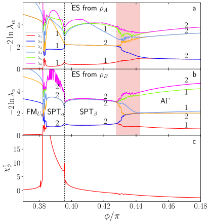
Figure 2: Entanglement spectrum and susceptibility for $\phi/\pi\mathord{<}0.5$. iDMRG results for: a Entanglement spectrum from $\rho_{A}$, red dashed line in Fig. 1a. b Entanglement spectrum from $\rho_{B}$, blue dashed line in Fig. 1a. The numbers refer to the degeneracy of the eigenvalue. c $\chi^{e}_{\phi}$. Two distinct phases, SPT_α and SPT_β, are visible between the FM${}_{U_{6}}$ and A$\Gamma$ phase. The red shading between $\phi/\pi$=0.428-0.442 denotes a transitional region of limited convergence due to a field instability.

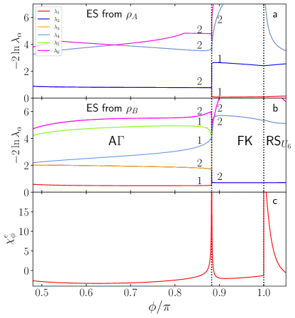
Figure 3: Entanglement spectrum and susceptibility for $\phi/\pi\mathord{>}0.5$. iDMRG results for: a Entanglement spectrum from $\rho_{A}$, red dashed line in Fig. 1a. b Entanglement spectrum from $\rho_{B}$, blue dashed line in Fig. 1a. The numbers refer to the degeneracy of the eigenvalue. c $\chi^{e}_{\phi}$. The A$\Gamma$  F$K$ and RS${}_{U_{6}}$ phases are clearly delineated.

Entanglement Spectrum

Our results for the entanglement spectrum, as well as for the susceptibility, $\chi^{e}_{\phi}$ are shown in Figs. 2 and 3. Due to the complexity of the phase diagram, we split it into two regions centered around the A$\Gamma$ phase: Fig.  2 represents the left part of the A$\Gamma$ and Fig. 3 the right part of the A$\Gamma$ phase. We consider two different partitions shown in Fig. 1a corresponding to $\rho_{A}$ and $\rho_{B}$. In both Fig. 2 and Fig. 3 iDMRG results are shown for both partitions with $\rho_{A}$ shown in panel (a) and $\rho_{B}$ in panel (b) with $\chi^{e}_{\phi}$ in panel (c).

To the left of the A$\Gamma$-phase, two other phases SPT_α and SPT_β are clearly separated from the FM${}_{U_{6}}$ and A$\Gamma$, as noted from their entanglement spectrum for $\rho_{A}$. Furthermore, the double degeneracy of the entanglement spectrum shown in Fig. 2 (b) from $\rho_{B}$ is a clear signal of a SPT phase [34, 35, 36, 37, 33]. Note that there is only a weak signature in $\chi^{e}_{\phi}$ of the transition between the two phases, visible at $\phi$=$0.3956\pi$ in Fig. 2(c), corresponding to a small discontinuity in $\chi^{e}_{\phi}$. While the FM${}_{U_{6}}$ phase appears abruptly at $\phi$=$0.3823\pi$, the transitions between the A$\Gamma$ phase and SPT_β phase at $\phi\sim 0.435\pi$ is not discernible in $\chi^{e}_{\phi}$. The blurriness of the transition is likely due to a field induced phase that pinches off to a single point at zero field at the A$\Gamma$-SPT_β transition, thereby obscuring it. We note that, the quantum critical points (QCPs) are immediately noticeable in the entanglement spectra.

Moving to the right within the A$\Gamma$ phase which encompass the point $\Gamma$ =1, the transition to the F$K$ phase from the A$\Gamma$ phase occurs at $\phi\mathord{=}0.88271(5)\pi$, which is clearly visible in the entanglement spectra as well as $\chi^{e}_{\phi}$ as shown in in Fig. 3. The transition between the RS${}_{U_{6}}$ and FK phases at $\phi$=$\pi$ is less apparent in the structure of the entanglement spectrum in Fig. 3 (a) and (b). However, from the results for $\chi^{e}_{\phi}$ in Fig. 3(c) this transition is immediately visible, and it was also noted that the second derivative of $\lambda_{1}$ clearly detects the transition [30].

Similar to the A$K$ phase, none of the phases SPT_α, SPT_β, A$\Gamma$ and F$K$ has any long-range magnetic ordering, nor is there any indication of nematic (quadropolar) or chiral ordering. As discussed in Supplementary Note 2, all four phases are gapped with a finite sizeable correlation length. The difference between them is captured in the entanglement spectrum. In the SPT_α, SPT_β and F$K$ (and A$K$) phases, the entanglement spectrum have all entries doubled when considering $\rho_{B}$. For the A$\Gamma$-phase, the same applies to the spectrum for $\rho_{A}$. Since an entanglement spectrum where all eigenvalues have degeneracy larger than one is a signature of a topological non-trivial phase, in the next section, we investigate the projective symmetry analysis to confirm their non-trivial topology prior to presenting associated non-local SOPs.

Projective Symmetry Analysis

With the SPT_α, SPT_β, A$\Gamma$ and F$K$ phases as potential SPT phases, it is of considerable interest to investigate the projective representations [37, 38, 39, 40, 41, 42, 33] $U$, of a site symmetry $\mathcal{R}$. This has been done for $S$=1 chains [37, 38, 39, 40, 41, 42] and ladders [43] and also for $S$=1/2 ladders [41, 44, 45, 46, 47]. The matrices $U$ can be obtained from the generalized transfer matrices in iDMRG calculations as described in Ref. 48.

For the K$\Gamma$ ladder, it is a significant simplification to consider the transformed model obtained after applying the $U_{6}$ transformation. This transformation maps the original Hamiltonian $H_{\mathrm{K}\Gamma}$ to the transformed ladder, denoted by $H_{\mathrm{K}\Gamma}^{U_{6}}$. Under the $U_{6}$ transformation the $x$, $y$ and $z$-bonds of the K$\Gamma$-ladder are transformed into anisotropic Heisenberg bonds, $x^{\prime}$, $y^{\prime}$ and $z^{\prime}$ in the following manner:

$$x^{\prime}\ :\ -KS^{x}_{i}S^{x}_{j}-\Gamma(S^{y}_{i}S^{y}_{j}+S^{z}_{i}S^{z}_{j})$$

$$y^{\prime}\ :\ -KS^{y}_{i}S^{y}_{j}-\Gamma(S^{x}_{i}S^{x}_{j}+S^{z}_{i}S^{z}_{j})$$

$$z^{\prime}\ :\ -KS^{z}_{i}S^{z}_{j}-\Gamma(S^{x}_{i}S^{x}_{j}+S^{y}_{i}S^{y}_{j})$$ (3)

In the transformed ladder $H_{\mathrm{K}\Gamma}^{U_{6}}$ model, the definition of $x^{\prime}$, $y^{\prime}$ and $z^{\prime}$-bonds, can pictorially be represented as shown in Fig. 4(a).

Figure 4: Unit cells of the $U_{6}$ transformed ladder. Two unit cells of $H_{\mathrm{K}\Gamma}^{U_{6}}$, the K$\Gamma$ ladder after the $U_{6}$ local transformation with $N\mathord{=}6n$ sites. a Two regular unit cells with regular open boundary conditions (OBC). b Two slanted unit cells with slanted OBC.

See Supplementary Note 1. We will consider two different open boundary conditions (OBC) as shown in Fig. 4. The unit cells depicted in panel (a) are referred to as regular unit cells with regular OBC, while the ones in panel (b) are referred to as slanted unit cells with slanted OBC.

In order to understand the symmetries of the matrix product state (MPS) wave-function, it is useful to write it in the canonical form [49, 50, 51, 52]:

$$|\Psi\rangle=\sum_{j_{1},\ldots,j_{N}}M^{[1]}_{j_{1}}\Lambda^{[2]}M^{[2]}_{j_{2}}\ldots\Lambda^{[N]}M^{[N]}_{j_{N}}|j_{1},\ldots,j_{N}\rangle,$$ (4)

where the $M^{[n]}_{j_{n}}$ are complex matrices and the $M^{[n]}$, real, positive, square diagonal matrices. In the iDMRG formulation, the set of matrices on any unit cell becomes the same $M^{[n]}_{j}$=$M_{j}$, $M^{[n]}$ = $M$ for all $n$, although they may vary within the unit cell. For the translationally invariant state, it can be shown [53, 34] that for any (site) symmetry operation $g$, represented in the spin basis by the unitary matrix, $\Sigma_{jj^{\prime}}(g)$, the $M_{j}$ matrices must transform as [34, 48]:

$$\sum_{j^{\prime}}\Sigma_{jj^{\prime}}(g)M_{j^{\prime}}=e^{i\theta}U^{\dagger}(g)M_{j}U(g),$$ (5)

where the unitary matrix $U(g)$ commutes with the $M$ matrices and $e^{i\theta}$ is a phase factor. With $D$ denoting the bond dimension, the $U$ matrices form a $D$-dimensional projective representation of the symmetry group of the wave-function, and they can be determined from the unique eigenvector of the generalized transfer matrix [34, 48] with eigenvalue $|\lambda|$=1, where the generalized transfer matrix is defined as

$$T^{\Sigma}_{\alpha\alpha^{\prime};\beta\beta^{\prime}}=\sum_{j}\left(\sum_{j^{\prime}}\Sigma_{jj^{\prime}}M_{j^{\prime},\alpha\beta}\right)(M_{j,\alpha^{\prime}\beta^{\prime}})^{*}\Lambda_{\beta}\Lambda_{\beta^{\prime}}$$ (6)

If the largest eigenvalue is $|\lambda|<$1, the symmetry is not a property of the state being considered. The projective representation is reflected in the fact that if $\Sigma(g)\Sigma(h)$=$\Sigma(gh)$, then

$$U(g)U(h)=e^{i\phi(g,h)}U(gh),$$ (7)

where the phases $\phi(g,h)$ are characteristic of the topological phase.

Let us now consider the site symmetries, $\mathcal{R}^{x}$ and $\mathcal{R}^{y}$ defined as:

$$\mathcal{R}^{x}_{l}=e^{i\pi S^{x}_{l}}\ ,\ \ \ \mathcal{R}^{y}_{l}=e^{i\pi S^{y}_{l}}\ ,\ \ \ \mathcal{R}^{z}_{l}=e^{i\pi S^{z}_{l}}.$$ (8)

The Hamiltonian $H_{\mathrm{K}\Gamma}^{U_{6}}$ is invariant under the operators $\prod_{l}\mathcal{R}^{\gamma}_{l}$, with $\gamma\mathord{=}x,y,z$ with distinct quantum numbers for the low-lying states. If these symmetries are respected, their representations can differ by a phase, $\phi(\mathcal{R}_{x},\mathcal{R}_{y})$ that must obey $e^{i\phi(\mathcal{R}_{x},\mathcal{R}_{y})}$=$\pm 1$:

$$U(\mathcal{R}^{x})U(\mathcal{R}^{y})=\pm U(\mathcal{R}^{y})U(\mathcal{R}^{x}).$$ (9)

Furthermore, the non-trivial value $e^{i\phi(\mathcal{R}_{x},\mathcal{R}_{y})}$=-1 can only occur if all eigenvalues of the entanglement spectrum are at least twice degenerate [34]. The phase factor can then be isolated by defining [48]:

$$\mathcal{O}_{\mathrm{Z_{2}\times Z_{2}}}\equiv\frac{1}{D}\operatorname{Tr}\left(U(\mathcal{R}^{x})U(\mathcal{R}^{y})U^{\dagger}(\mathcal{R}^{x})U^{\dagger}(\mathcal{R}^{y})\right),$$ (10)

with $D$ the bond dimension, with similar definitions for other pairs of operators in Eq. (8). In the above definitions it is understood that the transformations are applied throughout the lattice and in order to obtain the matrices $U$, generalized transfer matrices representing the relevant unit cell has to be considered.

The site symmetries, $\mathcal{R}^{x}$, $\mathcal{R}^{y}$ and $\mathcal{R}^{z}$, forming the dihedral group, $D_{2}$, are respected by both of the unit cells in Fig. 4(a) and 4(b). Using generalized transfer matrices obtained from unit cells of the shape shown in Fig 4(a) when studying the A$\Gamma$-phase and of the slanted shape shown in Fig. 4(b) when studying the F$K$, SPT_α, and SPT_β phases, we obtain

$$\mathcal{O}_{\mathrm{Z_{2}\times Z_{2}}}=-1,$$ (11)

for the SPT_α, SPT_β, A$\Gamma$, and F$K$ phases.

Similar analysis can be made for the time-reversal $(\mathrm{TR})$ symmetry, defined by $M_{j}\to\sum_{j^{\prime}}\left[e^{i\pi S^{y}}\right]_{jj^{\prime}}M^{\star}_{j^{\prime}}$, with $\star$ denoting complex conjugation. In this case, it can be established that [34] $U_{\mathrm{TR}}U_{\mathrm{TR}}^{\star}$=$e^{i\phi(\mathrm{TR},\mathrm{TR})}\mathbb{1}$ where the phase $\phi(\mathrm{TR},\mathrm{TR})$ cannot be absorbed into the definition of $U_{\mathrm{TR}}$. One should note that for most other symmetries, with the notable exception of inversion, similar considerations will lead to $U^{2}$=$e^{i\phi}\mathbb{1}$ in which case the phase $\phi$ in fact can be absorbed into the definition of $U$. For instance, this is the case for $U\left(\mathcal{R}^{\alpha}\right)$ discussed above. However, for time reversal, the phase factor $e^{i\phi(\mathrm{TR},\mathrm{TR})}$ can directly be extracted by defining [48]:

$$\mathcal{O}_{\mathrm{TR}}\equiv\frac{1}{D}\operatorname{Tr}\left(U_{\mathrm{TR}}U_{\mathrm{TR}}^{\star}\right),$$ (12)

and again one finds that $\phi(\mathrm{TR},\mathrm{TR})$=0,$\pi$, so that $\mathcal{O}_{\mathrm{TR}}$=$\pm$1. As an example, for the $S$=1 Heisenberg spin chain in the Haldane phase it is known that $\mathcal{O}_{\mathrm{Z_{2}\times Z_{2}}}$=$-1$, $\mathcal{O}_{\mathrm{TR}}$=$-1$ [34, 35].

Using generalized transfer matrices obtained from unit cells of the shape shown in Fig 4(a) for the A$\Gamma$-phase and of the slanted shape for the F$K$, SPT_α, and SPT_β phases, we obtain

$$\mathcal{O}_{\mathrm{TR}}=-1,$$ (13)

consistent with the presence of a doubled entanglement spectrum in all cases. As was the case for $\mathcal{O}_{\mathrm{Z_{2}\times Z_{2}}}$ , if the unit cells are interchanged, one finds instead $\mathcal{O}_{\mathrm{TR}}$=1.

Table 1: Summary of projective analysis. The superscript $\mathrm{regular}$ refers to the unit cell from Fig. 4a, while the superscript $\mathrm{slanted}$ refers to the unit cell from Fig. 4b. Negative values indicate that the state transforms non-trivially.

Phase	$\mathcal{O}_{\mathrm{TR}}^{\mathrm{regular}}$	$\mathcal{O}_{\mathrm{Z_{2}\times Z_{2}}}^{\mathrm{regular}}$	$\mathcal{O}_{\mathrm{TR}}^{\mathrm{slanted}}$	$\mathcal{O}_{\mathrm{Z_{2}\times Z_{2}}}^{\mathrm{slanted}}$
SPTα	1	1	-1	-1
SPTβ	1	1	-1	-1
A$\Gamma$	-1	-1	1	1
F$K$	1	1	-1	-1

A summary of our results from the projective analysis are provided in Table 1, negative values indicate that the state transforms non-trivially. For all 4 phases, it is seen that a unit cell can be chosen for which the state transforms non-trivially under both the $\mathrm{TR}$ and $\mathcal{O}_{\mathrm{Z_{2}\times Z_{2}}}$ symmetries.

Based on the above analysis of entanglement spectrum and projective symmetry, we conclude that A$\Gamma$ phase is an SPT phase. It is then important to further identify its SOP that differentiates this phase from the other disordered phases.

Twice Hidden String Order

To establish a non-local string order parameter (SOP) characterizing the A$\Gamma$ phase, we need to exploit a non-local unitary transformation that maps the original Hamiltonian with OBC to a new Hamiltonian that exhibits a local long-range order [54, 55, 56]. We found that it is difficult to identify such non-local transformation starting from the original $H_{\mathrm{K}\Gamma}$, but it can be achieved by first applying the $U_{6}$ transformation to arrive at $H_{\mathrm{K}\Gamma}^{U_{6}}$. It is then possible to define a non-local unitary transformation $W$, mapping $H_{\mathrm{K}\Gamma}^{U_{6}}$ to a new local Hamiltonian. We denote the resulting Hamiltonian, where four-spin terms appear, by $H_{\mathrm{KQ}}$. For the parameters relevant for the A$\Gamma$-phase, $H_{\mathrm{KQ}}$ exhibits long-range order in the spin-spin correlation functions, corresponding to a local order parameter. Due to the application of two separate unitary transformations, one might consider the resulting order to be twice hidden.

The non-local unitary operator $W$ for a $N$-site ladder with OBC that maps $H_{\mathrm{K}\Gamma}^{U_{6}}$ to $H_{\mathrm{KQ}}$ takes the following form.

$$W=\prod_{\begin{subarray}{c}j+1<k\\ j\ \mathrm{odd},\ k\ \mathrm{odd}\\ j=1,\ldots N-3\\ k=3,\ldots N-1\end{subarray}}w(j,k).$$ (14)

With the individual $w(j,k)$ given as follows:

$$w(j,k)=e^{i\pi(S^{y}_{j}+S^{y}_{j+1})\cdot(S^{z}_{k}+S^{z}_{k+1})},$$ (15)

and $W^{\dagger}$=$W$. The OBC are here crucial for the mapping to be exact. Evidently, all $w(j,k)$ are unitary and therefore also $W$, and $\left[w(j,k),w(l,m)\right]=0\ \ \forall\ j,k,l,m$. Note that this is a different labelling of the unitary operator introduced in Ref. [23, 30]. It can also be shown that other combinations of the spin operators $S^{\alpha}$ appearing in Eq. (15) lead to equivalent unitary operators, for instance, $e^{i\pi(S^{y}_{j}+S^{y}_{j+1})\cdot(S^{x}_{k}+S^{x}_{k+1})}$ is another valid choice. However, the specific choice made in Eq. (15) will influence the type of ordering that is observed in $H_{\mathrm{KQ}}$, as well as the specific form of $H_{\mathrm{KQ}}$. Schematically, the transformations can be viewed as shown in Fig. 5. The detailed form of $H_{\mathrm{KQ}}$ after the $W$ transformation on $H_{\mathrm{K}\Gamma}^{U_{6}}$ is presented in Supplementary Note 4.

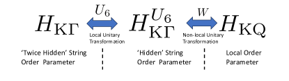
Figure 5: Pictorial view of KG transformations. The two transformations from the original K$\Gamma$ model to $H_{\mathrm{K}\Gamma}^{U_{6}}$, and the subsequent transformation to $H_{\mathrm{KQ}}$ are sketched. The type of order parameter for each Hamiltonian is indicated.

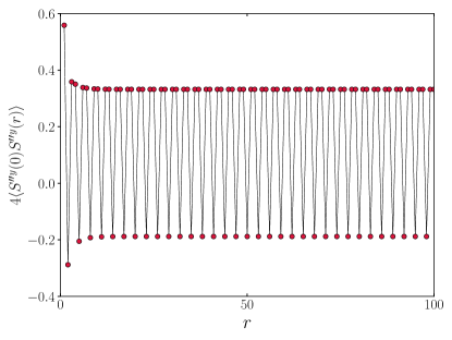
Figure 6: Spin correlations in the $H_{\mathrm{KQ}}$ model at $\phi\mathord{=}0.85\pi$. DMRG results with $N$=384 for the correlation function $4\langle S^{\prime\prime y}(0)S^{\prime\prime y}(r)\rangle$ versus distance, $r$ along one leg of the ladder. $r$=0 corresponds to site 47. Results are for $H_{\mathrm{KQ}}$ with $\phi\mathord{=}0.85\pi$ and $r$ is measured in lattice spacings along the leg.

We first discuss the ordering in $H_{\mathrm{KQ}}$ where we denote the spins by $S^{\prime\prime\alpha}$, where the double prime represents the two transformations of spin from the original Hamiltonian. It is then convenient to study correlation functions of the form $4\langle S^{\prime\prime\alpha}(0)S^{\prime\prime\alpha}(r)\rangle$ along the legs of the ladder with $r$ measured in lattice spacings along the leg. To avoid boundary effects, $r$=0 is usually taken to correspond to a site in the bulk of the chain. In Fig. 6 we show results for $4\langle S^{\prime\prime y}(0)S^{\prime\prime y}(r)\rangle$ starting from site 47 with $\phi\mathord{=}0.85\pi$. Long-range order is clearly present. Similar results can be obtained for the other leg of the ladder as well as for $4\langle S^{\prime\prime z}(0)S^{\prime\prime z}(r)\rangle$. However, due to the choice of spin operators in the definition of $w$ in Eq. (15), there is no ordering in $4\langle S^{\prime\prime x}(0)S^{\prime\prime x}(r)\rangle$.

Using the inverse of the non-local unitary operator $W$ from Eq. (14) the above results for $4\langle S^{\prime\prime y}(0)S^{\prime\prime y}(r)\rangle$ is reproduced as a non-local string order correlation function in $H_{\mathrm{K}\Gamma}^{U_{6}}$ where we denote the spin variables by $S^{\prime\alpha}$=$\sigma^{\prime\alpha}/2$. We find $\langle S_{1}^{\prime\prime y}S_{r+1}^{\prime\prime y}\rangle$ is given by

$${\cal O}^{y}(r) = 4\langle S_{1}^{\prime\prime y}S_{r+1}^{\prime\prime y}\rangle=(-1)^{\left\lfloor{r/2}\right\rfloor}$$ (19)

$$\times \left\{\begin{array}[]{rl}\langle\sigma_{2}^{\prime y}\left(\prod_{k=3}^{r}\sigma_{k}^{\prime y}\right)\sigma_{r+1}^{\prime y}\rangle&\mbox{ $r$ even}\\ \\ \langle\sigma_{2}^{\prime y}\left(\prod_{k=3}^{r-1}\sigma_{k}^{\prime y}\right)\sigma_{r+1}^{\prime y}\rangle&\mbox{ $r$ odd}\end{array}\right.$$

Note that, to fully reproduce the results for $H_{\mathrm{KQ}}$ shown in Fig. 6 with the string correlation function in (19) for $H_{\mathrm{K}\Gamma}^{U_{6}}$, a relabelling of the sites needs to be done that we have skipped for clarity.

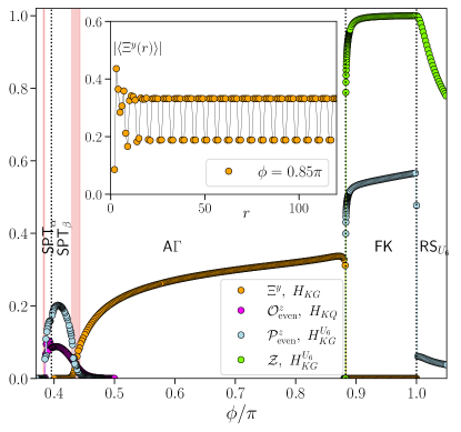
Figure 7: String order parameters in the A$\Gamma$ and surrounding phases. iDMRG results for the string order parameters in the $H_{\mathrm{K}\Gamma}$ and $H_{\mathrm{K}\Gamma}^{U_{6}}$ models, shown alongside DMRG results for $H_{\mathrm{KQ}}$. Orange circles, $\Xi^{y}$ for $H_{\mathrm{K}\Gamma}$. The inset shows $\Xi^{y}(r)$ versus $r$ at $\phi\mathord{=}0.85\pi$ for $H_{\mathrm{K}\Gamma}$. Magenta circles, DMRG results for ${\cal O}_{\mathrm{even}}^{z}$ for $H_{\mathrm{KQ}}$. Light blue circles, ${\cal P}^{z}_{\mathrm{even}}$ for $H_{\mathrm{K}\Gamma}^{U_{6}}$. Green circles, ${\cal Z}$ for $H_{\mathrm{K}\Gamma}^{U_{6}}$.

We can now apply the inverse $U_{6}$ transformation (see Supplementary Note 1) to the above expressions for ${\cal O}^{y}(r)$ to determine the string order correlation functions that define the A$\Gamma$-phase in the original $H_{\mathrm{K}\Gamma}$:

$$\Xi^{y}(r)=U_{6}^{-1}({\cal O}^{y}(r)),$$ (20)

with the $U_{6}^{-1}$ transformation detailed in Supplementary Note 1. The SOP in $H_{\mathrm{K}\Gamma}$ Hamiltonian is then given by

$$\Xi^{y}=\max_{r\to\infty}\Xi^{y}(r).$$ (21)

It is interesting to note that for a small $r$, for example $r=7$ $\Xi^{y}(r=7)$ corresponds to the plaquette operator found in the pure Gamma model in the honeycomb lattice.[57]

In Fig. 7 we show iDMRG results for $\Xi^{y}$ (orange circles). The inset shows iDMRG results for $\Xi^{y}(r)$ versus $r$ at $\phi\mathord{=}0.85\pi$ which at large $r$ can be compared to the results for $H_{\mathrm{KQ}}$ shown in Fig. 6. Note that the results in Fig. 6 show the correlations along a leg, whereas the inset in Fig. 7 show results from both legs without including the sign and the relabelling of the sites. Due to the different methods used, there is not an exact equivalence for very small values of $r$.

We emphasize that the appearance of a non-local SOP in the A$\Gamma$ phase of $H_{\mathrm{K}\Gamma}$ is equivalent to the presence of long-range order in $H_{\mathrm{KQ}}$. Hence, $\Xi^{y}$ is non-zero throughout the A$\Gamma$-phase and goes to zero at the critical points delineating this phase. It is absent in the other disordered phases, SPT_α, SPT_β, and F$K$, and thus uniquely defines the A$\Gamma$ phase.

With the identification of the A$\Gamma$-phase with regular long-range ordering in the $H_{\mathrm{KQ}}$ model, it is natural to ask if a regular (local) order parameter can also be identified for the SPT_α- and SPT_β-phases in the $H_{\mathrm{KQ}}$. However, all local order parameters that we have investigated have not shown any ordering in the SPT_α- and SPT_β-phases for $H_{\mathrm{KQ}}$. Extending the string-order correlation function defined for the $S\mathord{=}1$ Haldane chain, a heuristic string-order correlation function has been proposed for $S$=1/2 ladders by pairing two $S\mathord{=}1/2$ [58, 59]. Following the numbering of Fig. 1a, if $\tau_{i}^{\alpha}\mathord{=}S^{\alpha}_{2i}+S^{\alpha}_{2i+1}$ are the sum of two diagonally situated spins, one defines [58, 59]:

$${\cal O}_{\mathrm{even}}^{\alpha}(r)=\langle\tau_{i}^{\alpha}\exp(i\pi\sum_{l=i+1}^{i+r-1}\tau_{l}^{\alpha})\tau_{i+r}^{\alpha}\rangle.$$ (22)

The associated SOP is non-zero in the phase surrounding $\phi\mathord{=}0$ in $H_{\mathrm{KQ}}$ [30], corresponding to the AFM Kitaev (A$K$) phase in $H_{\mathrm{K}\Gamma}$. The magenta points in Fig. 7 show our results for ${\cal O}_{\mathrm{even}}^{z}$ for the $H_{\mathrm{KQ}}$ model, which clearly is non-zero in the SPT_α- and SPT_β-phases. This is consistent with the nonexistence of a local order parameter in these two phases for $H_{\mathrm{KQ}}$. We note that, due to the heuristic nature of ${\cal O}_{\mathrm{even}}^{z}$, it is not clear how to associate it with a local order in a related model. Since $H_{\mathrm{K}\Gamma}$ and $H_{\mathrm{K}\Gamma}^{U_{6}}$ are related by a local unitary transformation, any ordering in the SPT_α- and SPT_β-phases in either model would immediately be apparent in both, and we have not observed any for either model.

Building on the above results for ${\cal O}_{\mathrm{even}}^{z}$ for $H_{\mathrm{KQ}}$ we propose a closely related heuristic string order correlation function for $H_{\mathrm{K}\Gamma}^{U_{6}}$ in the following way: Define $l_{i}^{\alpha}\mathord{=}S^{\alpha}_{2i}-S^{\alpha}_{2i+1}$ as the difference of two diagonally situated spins, following the numbering from Fig. 1a. We then have

$${\cal P}_{\mathrm{even}}^{\alpha}(r)=\langle l_{i}^{\alpha}\exp(i\pi\sum_{l=i+1}^{i+r-1}\tau_{l}^{\alpha})l_{i+r}^{\alpha}\rangle,$$ (23)

with $\tau_{i}^{\alpha}\mathord{=}S^{\alpha}_{i,1}+S^{\alpha}_{i+1,2}$ as above. Results for ${\cal P}_{\mathrm{even}}^{z}$ versus $\phi$ obtained from iDMRG calculations with $H_{\mathrm{K}\Gamma}^{U_{6}}$ are shown in Fig. 7 as the light blue points. The F$K$, SPT_α and SPT_β-phases are clearly defined by a non-zero ${\cal P}_{\mathrm{even}}$. By applying $U_{6}^{-1}$ to the definition of ${\cal P}_{\mathrm{even}}$ it is straightforward to perform similar calculations using $H_{\mathrm{K}\Gamma}$ by evaluating $U_{6}^{-1}({\cal P}_{\mathrm{even}}^{\alpha}(r))$. Even though the definition ${\cal P}_{\mathrm{even}}$ is heuristic, we interpret this result as a verification of the SPT nature of the F$K$, SPT_α- and SPT_β-phases.

For the F$K$-phase, it is also instructive to consider an even simpler heuristic string order correlation function, $\mathcal{Z}$ defined as follows [22]:

$$\mathcal{Z}=\langle\prod_{i}^{i+r}\sigma_{i}^{z}\rangle$$ (24)

We consider this string correlator for $H_{\mathrm{K}\Gamma}^{U_{6}}$ or equivalently to $H_{\mathrm{K}\Gamma}$ through application of $U_{6}^{-1}$. Results for $\mathcal{Z}$ are shown in Fig. 7 versus $\phi$ (green points) as obtained from iDMRG calculations. Throughout the F$K$-phase $\mathcal{Z}$ is almost identical to 1, dropping to zero at the transition to the A$\Gamma$-phase. However, we note that $\mathcal{Z}$ remain sizable throughout much of the RS${}_{U_{6}}$-phase, reflecting its heuristic nature.

Edge states and response to magnetic field

Another signature of SPT phases is the presence of edge states under OBC related to a ground state degeneracy. For the SPT phases in the K$\Gamma$ ladder, it is clear from the degeneracy of the entanglement spectrum that we need to consider different shapes of clusters (regular vs. slanted OBCs) for the different SPT phases. In this section, we exclusively study the original Hamiltonian $H_{\mathrm{K}\Gamma}$ and do not consider $H_{\mathrm{K}\Gamma}^{U_{6}}$ nor $H_{\mathrm{KQ}}$. For A$\Gamma$ phase, we use $N\mathord{=}4n$ with the regular OBC and for the remaining SPT phases, we use the slanted OBC with $N\mathord{=}4n+2$ in order to have an equal number of the different bond types.

We first demonstrate the presence of edge states in the SPT phases. For the A$\Gamma$ phase, results for the 16 lowest states with the regular OBC at $\phi\mathord{=}0.85\pi$ are obtained using ED (see Supplementary Figure 7). Four low-lying states below the gap are clearly present. With increasing $N$, these 4 states quickly become degenerate while the gap stabilizes at a finite value. Similar results can be obtained for the A$K$ and F$K$ phase using the slanted cluster, and a degeneracy of 4 is also observed for this case (see Supplementary Figure 8). For the SPT_α- and SPT_β-phases, it has not been possible to produce reliable results in the same manner, likely due to the significantly larger correlation lengths.

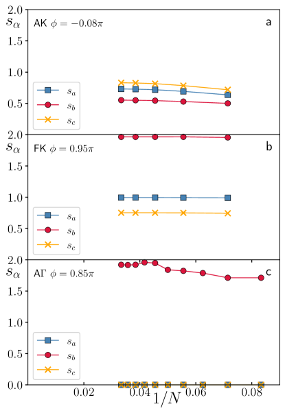
Figure 8: Eigenvalues of total spin in the A$K$, F$K$ and A$\Gamma$ phases. The eigenvalues $s_{\alpha}$=$s_{a,b,c}$ of the total spin $S_{\alpha}$=$\sum_{i}S^{\alpha}_{i}$ in the four degenerate ground-states, in zero field. Results are from ED. a A$K$-phase at $\phi=-0.08\pi$ with $N\mathord{=}14,18\ldots 30$ b F$K$-phase at $\phi=0.95\pi$ with $N\mathord{=}14,18\ldots 30$, c A$\Gamma$-phase at $\phi\mathord{=}0.85\pi$ with $N\mathord{=}12,14,\ldots 30$ (filled symbols).

To understand the nature of the edge-states, let us explore how the A$K$, F$K$, and A$\Gamma$ phases respond to an external magnetic field. An external magnetic field introduces an additional term in the Hamiltonian of the form $H^{\prime}\mathord{=}g_{L}\mu_{B}{\bf B}\cdot{\bf S}_{\mathrm{tot}}$, where ${\bf S}_{\mathrm{tot}}\mathord{=}\sum_{i}\mathbf{S}_{i}$, $g_{L}$ is the Landé factor and $\mu_{B}$ the Bohr magneton. Following Ref. [38] we denote the 4 states $\psi_{1},\psi_{2},\psi_{3}$ and $\psi_{4}$ and consider $\mathbf{S}_{\mathrm{tot},\alpha}$ in this four-fold degenerate space by defining

$$S^{\gamma\beta}_{\mathrm{tot},\alpha}=\langle\psi_{\gamma}|S_{\mathrm{tot},\alpha}|\psi_{\beta}\rangle,\ \ \gamma,\beta=1,2,3,4.$$ (25)

Here, the components of the total spin $S_{\mathrm{tot},\alpha}$ are usually taken to be identical to $x,y,z$ but given the underlying honeycomb structure we shall find it useful to instead consider $\alpha$=$\mathbf{\hat{a}}$, $\mathbf{\hat{b}}$, $\mathbf{\hat{c}}$ corresponding to the three directions $[$11-2$]$, $[$1-10$]$ and $[111]$ that correspond to the perpendicular and parallel to the z-bond, and perpendicular to the plane of the honeycomb (or n-leg brick-wall), respectively. One then finds that the eigenvalues of the matrices $(S^{\gamma\beta}_{\mathrm{tot},\alpha})$ for four corresponding degenerate states are simply given by $(s_{\alpha},-s_{\alpha},0,0)$.

Our ED results for $s_{\alpha}$ are shown in Fig. 8. For the A$K$ phase at $\phi\mathord{=-}0.08\pi$, shown in Fig. 8(a), we find $s_{a}\mathord{\sim}3/4$, $s_{b}\mathord{\sim}1/2$ and $s_{c}\mathord{\simeq}0.85$. Similarly, for the F$K$-phase at $\phi\mathord{=}0.95\pi$, shown in Fig. 8(b), we find $s_{a}$=1, $s_{b}\mathord{\sim}2$ and $s_{c}$=3/4. In both cases, we expect some variation in the values of $s_{\alpha}$ as $\phi$ is tuned. We note that for both the F$K$ and A$\Gamma$ phase, the values of $s_{\alpha}$ quickly saturate at a small, finite value as $N$ is increased. This is indicative of excitations localized at the edges as opposed to an actual magnetically ordered ground-state which should show $s_{\alpha}$ continually growing with $N$. A calculation of $s_{\alpha}$ for the SPT_α and SPT_β-phases do not yield clear results for the range of $N$ available with ED, as discussed in Supplementary Note 6. In a realistic experimental setting, the presence of impurities will always create finite open segments of ladders, with a resulting Curie-law behavior. The response to an applied magnetic field is in that case highly anisotropic and the low temperature Curie-law response should show a strong directional dependence [38, 41, 43] with $\chi_{a}(T)$, $\chi_{b}(T)$ and $\chi_{c}(T)$ clearly distinguishable. The results for the A$\Gamma$-phase, shown in Fig. 8(c), are even more intriguing. They are not only more anisotropic, but only $s_{b}$ is non-zero, approaching a value close to 2 at $\phi\mathord{=}0.85\pi$. At a slightly different point in the A$\Gamma$-phase with $\phi\mathord{=}0.8\pi$ we instead find $s_{b}\mathord{\simeq}4/3$ but again only $s_{b}$ is non-zero. This implies that the phase does not respond at all to a field applied along the $\mathbf{\hat{a}}$ and $\mathbf{\hat{c}}$ directions, effectively $g_{a},g_{c}\mathord{\simeq}0$.

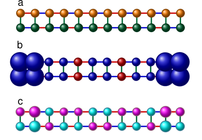
Figure 9: Ground state magnetization in an infinitesimal field in the A$\Gamma$ phase. ED results with $N$=24 for $\langle S^{a,b,c}_{i}\rangle$ in the lowest state in the AG phase at $\phi/\pi$=0.85 with a field in the $\mathbf{\hat{b}}$-direction of strength 0.002. The green, blue and cyan colors indicate positive values while orange, red, and pink indicate negative values. The size of the circles are proportional to the value of $\langle S^{a,b,c}_{i}\rangle$. a $\langle S^{a}_{i}\rangle$, b $\langle S^{b}_{i}\rangle$, c $\langle S^{c}_{i}\rangle$.

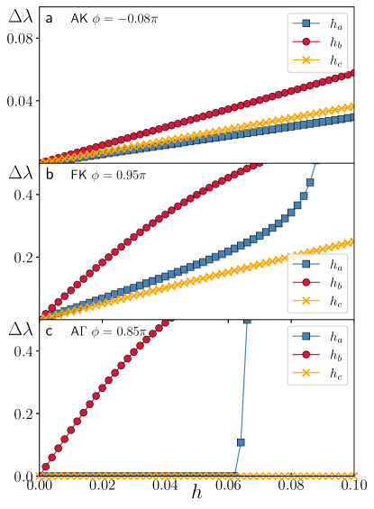
Figure 10: The Schmidt gap in the A$K$, F$K$ and A$\Gamma$ phases. The splitting of the entanglement spectrum $\Delta\mathord{=}\lambda_{1}\mathord{-}\lambda_{2}$ from iDMRG calculations with a field in the $\mathbf{\hat{a}}$, $\mathbf{\hat{b}}$ and $\mathbf{\hat{c}}$ directions. a A$K$-phase at $\phi=-0.08\pi$ using $\rho_{B}$. b F$K$-phase at $\phi=0.95\pi$ using $\rho_{B}$. c A$\Gamma$-phase at $\phi\mathord{=}0.85\pi$ using $\rho_{A}$.

To gain a clearer picture of how the ladder in the A$\Gamma$ phase responds to a magnetic field applied along the $\mathbf{\hat{b}}$-direction, we have performed ED calculations in the presence of a small field in the $\mathbf{\hat{b}}$-direction. The resulting site dependent magnetization $\langle S^{a,b,c}_{i}\rangle$ can then easily be obtained for the $\mathbf{\hat{a}},\mathbf{\hat{b}}$ and $\mathbf{\hat{c}}$-directions. Our results are shown in Fig. 9 for $N$=24 as obtained from the ground-state with a small field in the $\mathbf{\hat{b}}$-direction of 0.002 at $\phi/\pi$=0.85 in the A$\Gamma$-phase. The green, blue and cyan colors represent positive expectation values, whereas orange, red and pink colors indicate negative values, with the size of the points proportional to the expectation value. The response along the $\mathbf{\hat{a}}$, $\mathbf{\hat{c}}$ directions is completely symmetric in the positive and negative directions, yielding $\sum_{i}S^{a,c}_{i}$=0. However, along the $\mathbf{\hat{b}}$-direction the response is much larger, and we clearly find $\sum_{i}S^{b}_{i}\neq$0 consistent with the results shown in the SI (See Fig. S9) (c). With the field along the $\mathbf{\hat{b}}$-direction, sizeable excitations are visible at both ends of the ladder.

The response of the edge states to a magnetic field correlates with the lifting (or absence of lifting) of the degeneracy in the entanglement spectrum. As previously discussed, non-trivial indices in the projective analysis can only arise if the degeneracy of all states in the entanglement spectrum (ES) is larger than one. This implies that if a finite strength of the perturbation is needed to remove the degeneracy, then a phase transition does not occur until that strength is reached and the phase persists till that point. On the other hand, if the degeneracy is lifted for any non-zero strength of the perturbation, the symmetry protection is broken without an associated phase transition. We can then investigate the response of the degeneracy of the ES to a magnetic field in the $\mathbf{\hat{a}}$, $\mathbf{\hat{b}}$ and $\mathbf{\hat{c}}$ directions. This is shown in Fig. 10 for the A$K$, F$K$, and A$\Gamma$ phases. For simplicity, we focus exclusively on the difference in the two largest eigenvalues $\Delta\mathord{=}\lambda_{1}\mathord{-}\lambda_{2}$, and in each case we employ the reduced density matrix that has a two-fold degeneracy at zero field.

As can be seen in Fig. 10(a) the degeneracy in the ES for the A$K$ phase is immediately lifted by a field in any of the three directions which correlates with the response of the edge-states (See Fig. S9(a) in the SI). However, the response is rather weak, and a relatively large field has to be applied to see a significant splitting. For the F$K$ phase, we have a similar effect as shown in Fig. 10(b), but in this case the response is much stronger. However, for the A$\Gamma$ phase, where we show results in Fig. 10(c), it is clear that a field in the $\mathbf{\hat{a}}$ direction of around $h_{a}$=0.06 is needed to lift the degeneracy of the ES. For a field applied in the $\mathbf{\hat{c}}$ direction, a significantly larger field is needed. On the other hand, a field in the $\mathbf{\hat{b}}$ direction immediately induces a large splitting in the entanglement spectrum even for infinitesimal field strengths. Since the degeneracy remains intact in the $\mathbf{\hat{a}}$ and $\mathbf{\hat{c}}$ directions, we conclude that the SPT character of the A$\Gamma$ phase persists with respect to a field applied in the $\mathbf{\hat{a}}$ and $\mathbf{\hat{c}}$ directions.

The A$\Gamma$ phase is then protected by the product of time-reversal ($\mathrm{TR}$) and $\pi$ rotation around the $\mathbf{\hat{b}}$-axis ($\mathcal{R}_{b}$), $\mathrm{TR}\times\mathcal{R}_{b}$, the only remaining symmetry [60] when the field is in the ${\mathbf{\hat{a}}}{\mathbf{\hat{c}}}$ plane, but broken when it is along the ${\hat{b}}$-axis. Hence, if a field is applied in the ${\mathbf{\hat{a}}}{\mathbf{\hat{c}}}$ plane, a transition to the trivial polarized state can only occur at finite field strengths with potentially other phases intervening before the polarized state is encountered. Several such transitions were observed for the A$\Gamma$ phase (denoted by K$\Gamma$SL) for a field in the ${\mathbf{\hat{c}}}$ direction [18, 30]. On the other hand, the F$K$ phase is not protected by the $\mathrm{TR}\times\mathcal{R}_{b}$ symmetry, and if a field is applied in the ${\mathbf{\hat{c}}}$ direction the ES degeneracy is lost as shown in Fig. 10(b). However, the field induced F$K$ phase can still be distinguished from the polarized state.

Discussion

Our initial inquiry in this paper pertains to the nature of the A$\Gamma$ phase and whether there exists a defining quantity for its characterization. For example, the Kitaev phases (A$K$ and F$K$) in the ladder display the character of SPT phases. It is likely that A$\Gamma$ is another SPT phase. If so, we expect all the signatures of the SPT such as the degeneracy of the entanglement spectrum, ground state degeneracy under OBC, and the presence of a SOP. Using the iDMRG, DMRG, and ED techniques, we indeed found that the entanglement spectrum is degenerate and there exists four-fold ground state degeneracy under the regular OBC in the A$\Gamma$ phase. It is interesting to note that the same results were obtained for the Kitaev phases, A$K$ and F$K$, but under the slanted OBC.

Despite such clear signatures of the SPT, determining the corresponding SOP in the A$\Gamma$ phase has been challenging. We found that the string order correlation function is related to ordinary local order in a regular correlation function in a model $H_{\mathrm{KQ}}$ obtained only after two consecutive unitary transformations. Hence, we term this order as ’twice’ hidden.

To understand the symmetry that protects the A$\Gamma$ phase, we also investigated the effects of the external magnetic field. From the magnetic field response, we noted that the A$\Gamma$ phase is completely inert to the magnetic field when the field is applied in the ${\hat{a}}$ and ${\hat{c}}$ directions, which correspond to perpendicular to the z-bond and the ladder plane, respectively. Accordingly, the entanglement spectrum degeneracy remains intact when the field is applied in the ${\hat{a}}$ and ${\hat{c}}$ directions. This is in contrast to the effect of applying the magnetic field along the ${\hat{b}}$ direction, i.e., parallel to the z-bond, which immediately lifts the degeneracy of the entanglement spectrum. We note that the product of $\mathrm{TR}$ and $\mathcal{R}_{b}$, $\mathrm{TR}\times\mathcal{R}_{b}$ symmetry, is preserved when the magnetic field is applied in the ${\mathbf{\hat{a}}}{\mathbf{\hat{c}}}$-plane, which is valid for the generic honeycomb Kitaev model beyond the ladder[60]. Thus, we conclude that the A$\Gamma$ is protected by the $\mathrm{TR}\times\mathcal{R}_{b}$ symmetry. Another intriguing implication from the magnetic field study is that the edge state in the A$\Gamma$ phase is not a isotropic free spin-1/2 unlike the standard S=1 Haldane SPT. They act like spinless modes under the field in ${\hat{a}}$ and ${\hat{c}}$ directions. Further studies are needed to fully understand the nature of the zero-energy modes at the boundary of the system with the regular OBC.

In the context of Kitaev materials, let us revisit our motivations for investigating the A$\Gamma$ phase in the ladder model. As previously mentioned in the introduction, the majority of $d^{5}$ Kitaev materials prominently feature FM Kitaev and AFM $\Gamma$ interactions. However, ongoing debates persist regarding the specific phase that arises in this region. Several numerical studies have suggested the presence of magnetic disorder [12, 13, 14, 15, 16, 17, 18, 19], while others have indicated a magnetically ordered phase, such as a zig-zag order [21]. Should a zig-zag order indeed be manifest in the 2D limit, we would anticipate observing the same ordering pattern in the 2-leg ladder, as the magnetic unit cell of the zig-zag can be captured in the ladder geometry. This is indeed the case for the Kitaev-Heisenberg ladder model, where the zig-zag, stripy, and FM ordered phases reported in the 2D honeycomb clusters are found in the ladder geometry [23].

Our findings have substantiated the presence of disordered state in the A$\Gamma$ phase of the 2-leg ladder, categorizing it as a SPT phase characterized by a SOP. The 2D limit can be constructed by stacking the ladders, and one possibility of the resulting 2D phase is a stacked SPTs with edge modes known as a weak-SPT [61]. However, the coupling between the ladders may generate a new phase or critical point. It is interesting to note that the evolution from a stacked weak-SPT chains to a gapless critical point supporting edge modes that do not hybridize with bulk modes was reported in the extended anisotropic Kitaev model approaching from the dimer limit [62]. Our findings hint at the possibility that as the 2D limit is approached, the A$\Gamma$ phase may become a 2D spin liquid, denoted as the K$\Gamma$ spin liquid. However, we cannot rule out a possibility of large unit cell [63] or incommensurate [20] magnetic orders whose magnetic unit cells are beyond the ladder geometry, and a definitive resolution to this question remains a subject for future investigation.

Methods

.1 Numerical Methods

We use a fully parallelized implementation [64] of the Lanczos algorithm to perform the exact diagonalizations (ED) of ladders with up to $N$=30 using both open and periodic boundary conditions. In addition to exact diagonalizations, we use finite size density matrix renormalization group [65, 66, 67, 68, 69, 70] (DMRG) to study both the K$\Gamma$ model, Eq. (1) and $H_{\mathrm{K}\Gamma}^{U_{6}}$ under both periodic (PBC) and open (OBC) boundary conditions, with the main part of our results obtained from the infinite DMRG [71, 70] (iDMRG) variant of DMRG. The iDMRG calculations were performed with unit cells of 12, 24 or 60 sites. Typical precision for both DMRG and iDMRG are $\epsilon<10^{-11}$ with a bond dimension in excess of 1000.

.2 Energy susceptibility

To determine the phase diagram we study the susceptibility derived from the ground-state energy per spin, $e_{0}$:

$$\chi_{\phi}^{e}=-\frac{\partial^{2}e_{0}}{\partial\phi^{2}},\$$ (26)

At a quantum critical point (QCP) it is known [72] that, for a finite system of size $N$, the energy susceptibility diverges as

$$\chi^{e}\sim N^{2/\nu-(d+z)}.$$ (27)

Here $\nu$ and $z$ are the correlation and dynamical critical exponents and $d$ is the dimension. Hence, $\chi^{e}$ only diverges at the phase transition if the critical exponent $\nu$ is smaller than $2/(d+z)$. For the present case we have $d$=$1$ and if we assume $z$=1, then a divergence is observed only if $\nu<1$.

.3 Entanglement Entropy and Spectrum, Schmidt gap

When studying the ladder shown in Fig. 1a it is important to realize that there are different ways of partitioning the system in two partitions of size $x$ and $N-x$. This is crucial when considering the bipartite von Neumann entanglement entropy, $EE$, as well as for the entanglement spectrum [73] of central importance for understanding topological properties [73, 34, 74, 75]. Both are obtained from the spectrum of the reduced density matrix, $\rho_{x}$, of either one of the two partitions. Here we focus on two specific partitions shown in Fig. 1a as the red and blue dashed lines. With the numbering in Fig. 1a, they correspond to either an odd ($N/2$-1, red) or even ($N/2$, blue) number of sites in the partitions. We refer to the density matrix derived from the former case with $N/2$-1 as $\rho_{B}$ and to the latter case with $N/2$ as $\rho_{A}$. We mainly focus on the case where the number of sites in the partition is close to the mid-point, either $N/2-1$ ($\rho_{B}$) or $N/2$ ($\rho_{A}$). but when considering the bipartite entanglement entropy, we let the number in the partition vary but only consider an even number of sites in the sub system corresponding to moving the blue dashed line in Fig. 1a along the ladder. For a subsystem, $A$, of size $x$ the entanglement entropy is defined by:

$$EE(x)=-\mathrm{Tr}\rho_{x}\ln\rho_{x}.$$ (28)

Our results for $EE(x)$ can be found in Supplementary Note 2. The eigenvalues, $l_{\alpha}$, of the reduced density matrix, $\rho_{x}$, correspond to the Schmidt decomposition, $l_{\alpha}$=$\lambda_{\alpha}^{2}$ and thereby the entanglement spectrum [73], which then will depend on whether $\rho_{A}$ or $\rho_{B}$ from Fig. 1a is used. The Schmidt gap is then defined as $\lambda_{1}-\lambda_{2}$.

Data Availability

The data that support the findings of this study are available at 10.5281/zenodo.10443031, or alternatively from the corresponding authors upon reasonable request.

Code Availability

The code used to generate the data used in this study is available from the corresponding author upon reasonable request.

Author contributions

Density-matrix renormalization group and exact diagonalization calculations were performed by E.S.S. H.-Y. K. initiated the project. All authors managed the project and wrote the manuscript.

Competing Interests

The authors declare no Competing Financial or Non-Financial Interests.

See pages 1, of SI.pdf See pages 0, of SI.pdf

References

- [1] Witczak-Krempa, W., Chen, G., Kim, Y. B. & Balents, L. Correlated quantum phenomena in the strong spin-orbit regime. Annu. Rev. of Condens. Matter Phys. 5, 57–82 (2014).
- [2] Rau, J. G., Lee, E. K.-H. & Kee, H.-Y. Spin-orbit physics giving rise to novel phases in correlated systems: Iridates and related materials. Annu. Rev. of Condens. Matter Phys. 7, 195–221 (2016).
- [3] Takagi, H., Takayama, T., Jackeli, G., Khaliullin, G. & Nagler, S. E. Concept and realization of Kitaev quantum spin liquids. Nat. Rev. Phys. 1, 264–280 (2019).
- [4] Trebst, S. & Hickey, C. Kitaev materials. Phys. Rep. 950, 1–37 (2022).
- [5] Rousochatzakis, I., Perkins, N. B., Luo, Q. & Kee, H.-Y. Beyond kitaev physics in strong spin-orbit coupled magnets. Preprint at http://arxiv.org/abs/2308.01943 (2023).
- [6] Rau, J. G., Lee, E. K.-H. & Kee, H.-Y. Generic spin model for the honeycomb iridates beyond the Kitaev limit. Phys. Rev. Lett. 112, 077204 (2014).
- [7] Kitaev, A. Anyons in an exactly solved model and beyond. Ann. Phys. 321, 2–111 (2006).
- [8] Jackeli, G. & Khaliullin, G. Mott insulators in the strong spin-orbit coupling limit: From Heisenberg to a quantum compass and Kitaev models. Phys. Rev. Lett. 102, 017205 (2009).
- [9] Janssen, L., Andrade, E. C. & Vojta, M. Magnetization processes of zigzag states on the honeycomb lattice: Identifying spin models for -RuCl3 and Na2IrO3. Phys. Rev. B 96, 064430 (2017).
- [10] Winter, S. M. & et al. Models and materials for generalized Kitaev magnetism. J. Condens. Matter Phys. 29, 493002 (2017).
- [11] Hermanns, M., Kimchi, I. & Knolle, J. Physics of the Kitaev model: Fractionalization, dynamic correlations, and material connections. Annu. Rev. of Condens. Matter Phys. 9, 17–33 (2018).
- [12] Catuneanu, A., Yamaji, Y., Wachtel, G., Kim, Y. B. & Kee, H.-Y. Path to stable quantum spin liquids in spin-orbit coupled correlated materials. npj Quantum Mater. 3, 23 (2018).
- [13] Gohlke, M., Wachtel, G., Yamaji, Y., Pollmann, F. & Kim, Y. B. Quantum spin liquid signatures in Kitaev-like frustrated magnets. Phys. Rev. B 97, 075126 (2018).
- [14] Gohlke, M., Chern, L. E., Kee, H.-Y. & Kim, Y. B. Emergence of nematic paramagnet via quantum order-by-disorder and pseudo-goldstone modes in kitaev magnets. Phys. Rev. Res. 2, 043023 (2020).
- [15] Yamada, T., Suzuki, T. & Suga, S.-I. Ground-state properties of the model on a honeycomb lattice. Phys. Rev. B 102, 024415 (2020).
- [16] Lee, H.-Y. & et al. Magnetic field induced quantum phases in a tensor network study of Kitaev magnets. Nat. Commun. 11, 1639 (2020).
- [17] Luo, Q., Zhao, J., Kee, H.-Y. & Wang, X. Gapless quantum spin liquid in a honeycomb magnet. npj Quantum Mater. 6, 57 (2021).
- [18] Gordon, J. S., Catuneanu, A., Sørensen, E. S. & Kee, H.-Y. Theory of the field-revealed Kitaev spin liquid. Nat. Commun. 10, 2470 (2019).
- [19] Yilmaz, F., Kampf, A. P. & Yip, S. K. Phase diagrams of kitaev models for arbitrary magnetic field orientations. Phys. Rev. Res. 4, 043024 (2022).
- [20] Buessen, F. L. & Kim, Y. B. Functional renormalization group study of the kitaev- model on the honeycomb lattice and emergent incommensurate magnetic correlations. Phys. Rev. B 103, 184407 (2021).
- [21] Wang, J., Normand, B. & Liu, Z.-X. One proximate Kitaev spin liquid in the model on the honeycomb lattice. Phys. Rev. Lett. 123, 197201 (2019).
- [22] Feng, X.-Y., Zhang, G.-M. & Xiang, T. Topological characterization of quantum phase transitions in a spin- model. Phys. Rev. Lett. 98, 087204 (2007).
- [23] Catuneanu, A., Sørensen, E. S. & Kee, H.-Y. Nonlocal string order parameter in the Kitaev-Heisenberg ladder. Phys. Rev. B 99, 195112 (2019).
- [24] Yang, W., Nocera, A., Tummuru, T., Kee, H.-Y. & Affleck, I. Phase diagram of the spin- Kitaev-Gamma chain and emergent su(2) symmetry. Phys. Rev. Lett. 124, 147205 (2020).
- [25] Yang, W., Nocera, A., Sørensen, E. S., Kee, H.-Y. & Affleck, I. Classical spin order near the antiferromagnetic Kitaev point in the spin- Kitaev-Gamma chain. Phys. Rev. B 103, 054437 (2021).
- [26] Luo, Q., Zhao, J., Wang, X. & Kee, H.-Y. Unveiling the phase diagram of a bond-alternating spin- chain. Phys. Rev. B 103, 144423 (2021).
- [27] Sørensen, E. S., Gordon, J., Riddell, J., Wang, T. & Kee, H.-Y. Field-induced chiral soliton phase in the kitaev spin chain. Phys. Rev. Res. 5, L012027 (2023).
- [28] Sørensen, E. S., Riddell, J. & Kee, H.-Y. Islands of chiral solitons in integer-spin kitaev chains. Phys. Rev. Res. 5, 013210 (2023).
- [29] Chaloupka, J. c. v. & Khaliullin, G. Hidden symmetries of the extended Kitaev-Heisenberg model: Implications for the honeycomb-lattice iridates . Phys. Rev. B 92, 024413 (2015).
- [30] Sørensen, E. S., Catuneanu, A., Gordon, J. S. & Kee, H.-Y. Heart of entanglement: Chiral, nematic, and incommensurate phases in the Kitaev-Gamma ladder in a field. Phys. Rev. X 11, 011013 (2021).
- [31] Wen, X. G. Topological order in rigid states. Int. J. Mod. Phys. B4, 239 – 271 (1990).
- [32] Gu, Z.-C. & Wen, X.-G. Tensor-entanglement-filtering renormalization approach and symmetry-protected topological order. Phys. Rev. B 80, 155131 (2009).
- [33] Wen, X.-G. Colloquium: Zoo of quantum-topological phases of matter. Rev. Mod. Phys. 89, 041004 (2017).
- [34] Pollmann, F., Turner, A. M., Berg, E. & Oshikawa, M. Entanglement spectrum of a topological phase in one dimension. Phys. Rev. B 81, 064439 (2010).
- [35] Pollmann, F., Berg, E., Turner, A. M. & Oshikawa, M. Symmetry protection of topological phases in one-dimensional quantum spin systems. Phys. Rev. B 85, 075125 (2012).
- [36] Schuch, N., Pérez-García, D. & Cirac, I. Classifying quantum phases using matrix product states and projected entangled pair states. Phys. Rev. B 84, 165139 (2011).
- [37] Chen, X., Gu, Z.-C. & Wen, X.-G. Classification of gapped symmetric phases in one-dimensional spin systems. Phys. Rev. B 83, 035107 (2011).
- [38] Liu, Z.-X., Liu, M. & Wen, X.-G. Gapped quantum phases for the spin chain with symmetry. Phys. Rev. B 84, 075135 (2011).
- [39] Chen, X., Gu, Z.-C. & Wen, X.-G. Complete classification of one-dimensional gapped quantum phases in interacting spin systems. Phys. Rev. B 84, 235128 (2011).
- [40] Liu, Z.-X., Chen, X. & Wen, X.-G. Symmetry-protected topological orders of one-dimensional spin systems with symmetry. Phys. Rev. B 84, 195145 (2011).
- [41] Liu, Z.-X., Yang, Z.-B., Han, Y.-J., Yi, W. & Wen, X.-G. Symmetry-protected topological phases in spin ladders with two-body interactions. Phys. Rev. B 86, 195122 (2012).
- [42] Chen, X., Gu, Z.-C., Liu, Z.-X. & Wen, X.-G. Symmetry protected topological orders and the group cohomology of their symmetry group. Phys. Rev. B 87, 155114 (2013).
- [43] Chen, J.-Y. & Liu, Z.-X. Symmetry protected topological phases in spin-1 ladders and their phase transitions. Annals of Physics 362, 551–567 (2015).
- [44] Ueda, H. & Onoda, S. Symmetry-protected topological phases and transition in a frustrated spin- XXZ chain. Phys. Rev. B 90, 214425 (2014).
- [45] Kariyado, T. & Hatsugai, Y. Topological order parameters of the spin- dimerized Heisenberg ladder in magnetic field. Phys. Rev. B 91, 214410 (2015).
- [46] Ogino, T., Furukawa, S., Kaneko, R., Morita, S. & Kawashima, N. Symmetry-protected topological phases and competing orders in a spin- XXZ ladder with a four-spin interaction. Phys. Rev. B 104, 075135 (2021).
- [47] Ogino, T., Kaneko, R., Morita, S. & Furukawa, S. Ground-state phase diagram of a spin- frustrated XXZ ladder. Phys. Rev. B 106, 155106 (2022).
- [48] Pollmann, F. & Turner, A. M. Detection of symmetry-protected topological phases in one dimension. Phys. Rev. B 86, 125441 (2012).
- [49] Vidal, G. Efficient classical simulation of slightly entangled quantum computations. Phys. Rev. Lett. 91, 147902 (2003).
- [50] Vidal, G. Classical simulation of infinite-size quantum lattice systems in one spatial dimension. Phys. Rev. Lett. 98, 070201 (2007).
- [51] Pérez-García, D., Verstraete, F., Wolf, M. M. & Cirac, J. I. Matrix product state representations. Quantum Inf. Comput. 7, 401 (2007).
- [52] Orús, R. & Vidal, G. Infinite time-evolving block decimation algorithm beyond unitary evolution. Phys. Rev. B 78, 155117 (2008).
- [53] Pérez-García, D., Wolf, M. M., Sanz, M., Verstraete, F. & Cirac, J. I. String order and symmetries in quantum spin lattices. Phys. Rev. Lett. 100, 167202 (2008).
- [54] Kennedy, T. & Tasaki, H. Hidden symmetry breaking and the Haldane phase in S=1 quantum spin chains. Commun. Math. Phys. 147, 431–484 (1992).
- [55] Kennedy, T. & Tasaki, H. Hidden Z2xZ2 symmetry breaking in Haldane-gap antiferromagnets. Phys.Rev. B45, 304–307 (1992).
- [56] Oshikawa, M. Hidden symmetry in quantum spin chains with arbitrary integer spin. J. Condens. Matter Phys. 4, 7469–7488 (1992).
- [57] Rousochatzakis, I. & Perkins, N. B. Classical spin liquid instability driven by off-diagonal exchange in strong spin-orbit magnets. Phys. Rev. Lett. 118, 147204 (2017).
- [58] Kim, E. H., Fath, G., Sólyom, J. & Scalapino, D. J. Phase transitions between topologically distinct gapped phases in isotropic spin ladders. Phys. Rev. B 62, 14965–14974 (2000).
- [59] Fath, G., Legeza, Ö. & Sólyom, J. String order in spin liquid phases of spin ladders. Phys. Rev. B 63, 1525–5 (2001).
- [60] Cen, J. & Kee, H.-Y. Determining kitaev interaction in spin- honeycomb mott insulators. Phys. Rev. B 107, 014411 (2023).
- [61] You, Y., Devakul, T., Burnell, F. J. & Sondhi, S. L. Subsystem symmetry protected topological order. Phys. Rev. B 98, 035112 (2018).
- [62] Nanda, A., Agarwala, A. & Bhattacharjee, S. Phases and quantum phase transitions in the anisotropic antiferromagnetic kitaev-heisenberg- magnet. Phys. Rev. B 104, 195115 (2021).
- [63] Rayyan, A., Luo, Q. & Kee, H.-Y. Extent of frustration in the classical kitaev- model via bond anisotropy. Phys. Rev. B 104, 094431 (2021).
- [64] Läuchli, A. M., Sudan, J. & Sørensen, E. S. Ground-state energy and spin gap of spin- kagomé-heisenberg antiferromagnetic clusters: Large-scale exact diagonalization results. Phys. Rev. B 83, 212401 (2011).
- [65] White, S. R. & Noack, R. M. Real-space quantum renormalization groups. Phys. Rev. Lett. 68, 3487–3490 (1992).
- [66] White, S. R. Density matrix formulation for quantum renormalization groups. Phys. Rev. Lett. 69, 2863–2866 (1992).
- [67] White, S. R. Density-matrix algorithms for quantum renormalization groups. Phys. Rev. B 48, 10345–10356 (1993).
- [68] Schollwöck, U. The density-matrix renormalization group. Rev. Mod. Phys. 77, 259–315 (2005).
- [69] Hallberg, K. A. New trends in density matrix renormalization. Advances in Physics 55, 477–526 (2006).
- [70] Schollwöck, U. The density-matrix renormalization group in the age of matrix product states. Ann. Phys. 326, 96 – 192 (2011). January 2011 Special Issue.
- [71] McCulloch, I. P. Infinite size density matrix renormalization group, revisited. Preprint at https://arxiv.org/abs/0804.2509 (2008).
- [72] Albuquerque, A. F., Alet, F., Sire, C. & Capponi, S. Quantum critical scaling of fidelity susceptibility. Phys. Rev. B 81, 064418 (2010).
- [73] Li, H. & Haldane, F. D. M. Entanglement spectrum as a generalization of entanglement entropy: Identification of topological order in non-abelian fractional quantum hall effect states. Phys. Rev. Lett. 101, 010504 (2008).
- [74] Cho, G. Y., Ludwig, A. W. W. & Ryu, S. Universal entanglement spectra of gapped one-dimensional field theories. Phys. Rev. B 95, 115122 (2017).
- [75] Cho, G. Y., Shiozaki, K., Ryu, S. & Ludwig, A. W. W. Relationship between symmetry protected topological phases and boundary conformal field theories via the entanglement spectrum. J. Phys. A Math. Theor. 50, 304002 (2017).
- [76] Fishman, M., White, S. R. & Stoudenmire, E. M. The ITensor Software Library for Tensor Network Calculations. SciPost Phys. Codebases 4 (2022).
Acknowledgements.
We thank A. Catuneanu and J. Gordon for fruitful discussions during the initial stages of this work. We acknowledge the support of the Natural Sciences and Engineering Research Council of Canada (NSERC) through Discovery Grants (No. RGPIN-2017-05759 and No. RGPIN-2022-04601). H.-Y.K. acknowledges the support of CIFAR and the Canada Research Chairs Program. This research was enabled in part by support provided by SHARCNET (sharcnet.ca) and the Digital Research Alliance of Canada (alliancecan.ca). Part of the numerical calculations were performed using the ITensor library [76].Author contributions