Quantum coherence and the principle of microscopic reversibility

Abstract

The principle of microscopic reversibility is a fundamental element in the formulation of fluctuation relations and the Onsager reciprocal relations. As such, a clear description of whether and how this principle is adapted to the quantum mechanical scenario might be essential to a better understanding of nonequilibrium quantum processes. Here, we propose a quantum generalization of this principle, which highlights the role played by coherence in the symmetry relations involving the probability of observing a quantum transition and that of the corresponding time reversed process. We study the implications of our findings in the framework of a qubit system interacting with a thermal reservoir, and implement an optical experiment that simulates the dynamics. Our theoretical and experimental results show that the influence of coherence is more decisive at low temperatures and that the maximum departure from the classical case does not take place for maximally coherent states. Classical predictions are recovered in the appropriate limits.

Keywords: Microreversibility principle; quantum coherence; nonequilibrium quantum processes.

I Introduction

Fluctuation theorems (FT) are known to describe many general aspects of nonequilibrium thermal processes, and to bridge the gap between the reversible properties of the fundamental laws of physics and the irreversible nature of the macroscopic world evans ; jarz ; crooks ; jarz2 . Nevertheless, despite their importance in fundamental physics and wide range of applicability in the study of many-particle systems, FT are formulated based only on two elements: the assumption of the Gibbs canonical ensemble to represent thermal equilibrium systems and the principle of microscopic reversibility crooks2 ; campisi . The first concept is extensively discussed in many statistical mechanics textbooks, whereas the second, which is less widespread, predicts a symmetry relation between the probability of observing a given trajectory of a system through phase space and that of observing the time-reversed trajectory groot ; chandler . The microreversibility principle also plays a central role in the derivation of the celebrated Onsager reciprocal relations onsager1 ; onsager2 .

With the rapidly growing field of quantum thermodynamics, there has been an increasing effort to better understand FT when quantum effects become relevant talkner ; esposito ; aberg ; manzano ; kwon ; khan ; aguilar . In this regard, one natural strategy is to initially investigate whether and how the principle of microscopic reversibility is modified by this classical-to-quantum transition. Unlike the classical domain, in the quantum regime we cannot know the simultaneous position and momentum of a particle with certainty, which obscures the very notion of trajectory, and it is also possible the formation of nonclassical correlations between system and environment upon interaction deffner ; binder . However, one can alternatively define stochastic trajectories of a quantum state in the Hilbert space to represent the dynamics of an open quantum system, whose interactions with the environment are conceptualized as generalized measurements breuer . Still, depending on the commutation relation between the operators of the Hamiltonian of the system and those of the observables measured in an experiment, quantum coherence in the energy eigenbasis has to be considered, which prevents the system from having a well-defined energy korz ; francica ; santos ; bert . In a recent study of the interaction between coherent and thermal states of light in a beam-splitter, Bellini et al. verified the influence of quantum effects on the microreversibility condition, mainly in the low-temperature limit bellini .

Apart from being of central importance to the study of FT in the presence of quantum effects, so far very few works have addressed the microreversibility condition from a quantum-mechanical point of view bellini ; agarwal1973open ; nakamura2011fluctuation ; tolman1925principle . In this work, we propose a quantum generalization of the principle of microscopic reversibility. We consider the backward process of the system as resulting from the inverse unitary protocol applied to both system and reservoir, which connects the time-reversed states of the final and initial states of the forward process. To test our model, we examine the dynamics of a two-level system coupled to a thermal reservoir at finite temperature, paying special attention to the mechanism in which the coherence influences the symmetry relation between forward and backward quantum trajectories. We also use an optical setup to simulate the open quantum system dynamics. Our setup allows the preparation of the system in an arbitrary qubit state and the realization of projective measurements onto states with coherence. The experimental data agree with our theoretical predictions, which confirm that the influence of coherence is more prominent at low temperatures, but in a nontrivial way. Our results recover the classical predictions in the appropriate limit.

Our paper is structured as follows. We begin in Sec. II by briefly reviewing the principle of microscopic reversibility as applied to the simple case of a classical gas. In Sec. III, we present our quantum-mechanical approach to the principle, and employ it to study the thermalization process of a qubit system interacting with a finite temperature environment. In Sec. IV, we use our results to evidence the effect of coherence in the departure of our proposed quantum microreversibility relation from the classical picture. Sec. V describes our experimental setup, in which we simulate the qubit thermalization example and investigate the role played by coherence in the quantum microscopic reversibility condition. We conclude in Sec. VI with a summary of our theoretical and experimental findings.

II Principle of microscopic reversibility

To begin, lets consider the rather simple but important scenario where the system is a classical gas in a container in contact with a thermal reservoir, in which some time-dependent parameter $\lambda(t)$ is controlled. In this case, the system can exchange heat $Q$ with the reservoir, and the manipulation of the control parameter may result in work $W$ being supplied to the system. To better illustrate this picture, let us assume a gas confined in a container with diathermic walls through which heat can be exchanged with the surroundings, and the work parameter $\lambda$ can be considered as the position of a movable piston, as depicted in Fig. 1. We define $z(t)$ as the time-dependent state of the system, which in our example is represented by a vector that determines all the instantaneous positions and momenta of the gas particles. Therefore, given the initial state $z_{i}$ and a protocol $\lambda(t)$, the dynamics of the system is completely specified by a trajectory $z(t)$ in the phase space, leading to a final state $z_{f}$.

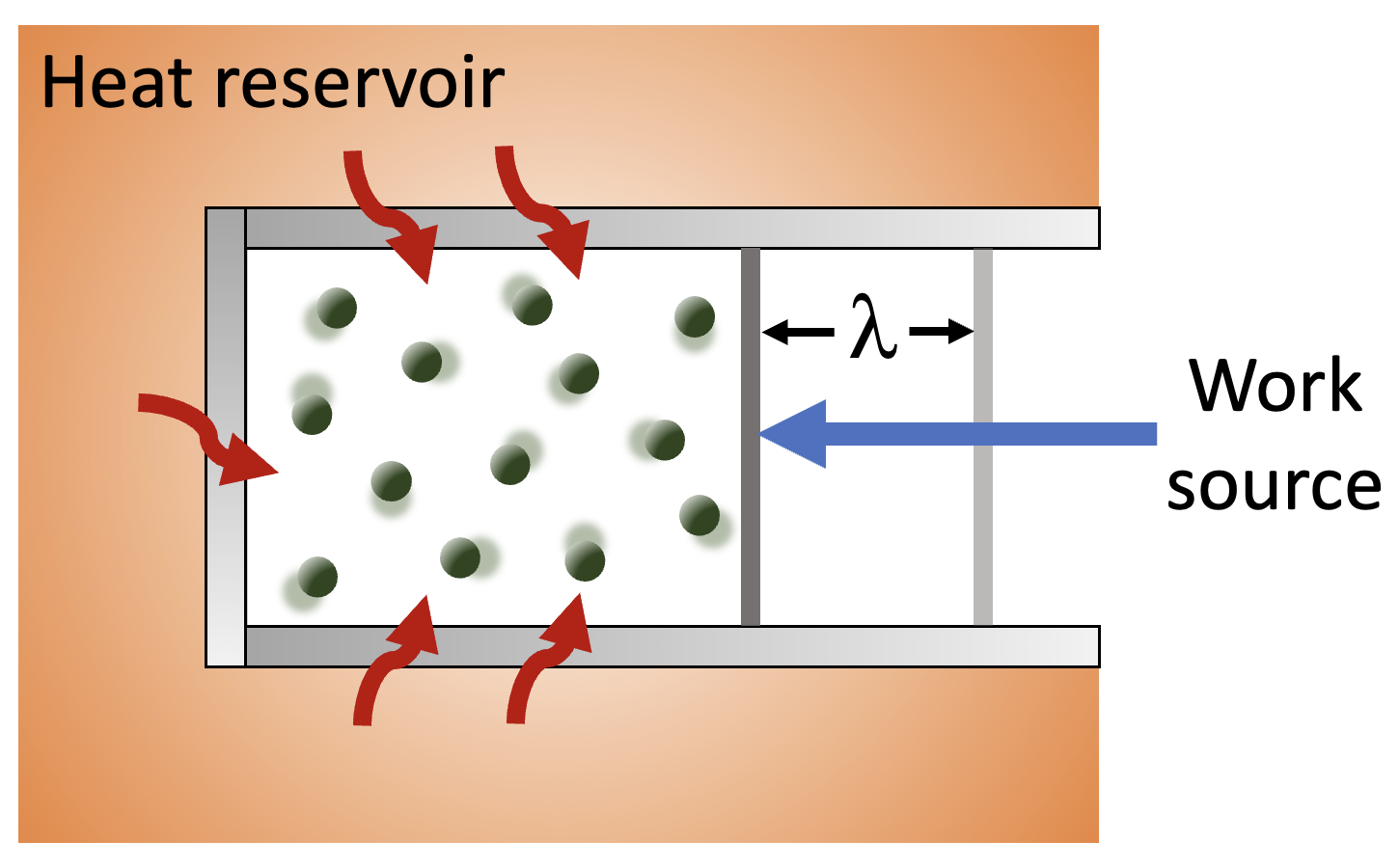
Figure 1: Gas particles inside a container representing a general thermodynamic system. Transfer of heat between the gas and the reservoir is allowed through the boundary walls, and a work source acts by manipulating the position $\lambda$ of the movable piston.

On the other hand, we can also define a reverse trajectory $\bar{z}(t)$, which can be visualized as a movie of the forward trajectory $z(t)$ played backwards. In this case, the process starts with the system in the state $\bar{z}_{f}$ and ends in the state $\bar{z}_{i}$. Here, an arbitrary state $\bar{z}$ is produced by keeping the position of all particles of the state $z$ unchanged, but reversing the sign of all the momenta. If we assume that in the forward trajectory the system starts in the state $z_{i}$ at time $0$ and attains $z_{f}$ at time $\tau$, the reverse protocol of the work parameter satisfies $\bar{\lambda}(\tau-t)=\lambda(t)$. We also consider that the heat reservoir is in thermal equilibrium during the entire process $z(t)$, so that it has the same influence on the system, independent of being in a forward or backward dynamics. With these definitions, the principle of microscopic reversibility states that the ratio of the probability of the forward trajectory from $z_{i}$ to $z_{f}$ to the probability of the corresponding backward trajectory from $\bar{z}_{f}$ to $\bar{z}_{i}$ is given by crooks ; crooks2 ; groot :

$$\frac{P_{F}(z_{f}|z_{i})}{P_{B}(\bar{z}_{i}|\bar{z}_{f})}=e^{-\beta Q},$$ (1)

where $Q$ is the heat absorbed by the system from the surroundings during the forward path, and $\beta=1/(k_{B}T)$, with $k_{B}$ the Boltzmann constant and $T$ the temperature of the reservoir. This relation reveals that the probability of occurring a particular trajectory that generates dissipation ($Q<0$) is exponentially greater than that of the corresponding reverse trajectory. If the control parameter is fixed and the gas is in thermal equilibrium with the reservoir, we have that $Q=0$. In this case Eq. (1) tells us that the probability of observing any given forward trajectory is equal to that of observing the corresponding backward trajectory.

III Quantum microscopic reversibility

Based on the ideas presented in the previous section, we now investigate how the principle of microscopic reversibility can be extended to the realm of individual quantum trajectories with the control parameter kept constant, i.e., without the realization of work. At this level, some strictly quantum-mechanical conditions have to be considered. First, as already mentioned, the notion of quantum trajectory is not well defined sakurai , but alternative approaches have been proposed, as for example the two-point measurement (TPM) protocol Talkner_2007 , which is the framework to be used here. Second, quantum measurements cause dynamical changes in the system that are never observed in classical objects jauch1964problem ; muller2023six . Third, depending on the commutation relation between the measured observables and the Hamiltonian of the system, the quantum dynamics could start or end in a state with coherence in the energy eigenbasis. In light of this freedom, the study of the influence of the initial and final coherence of the system on the microscopic reversibility relation is our main focus here.

Let us now present the quantum mechanical framework we use to study the microscopic reversibility. We consider a qubit system in contact with a large thermal reservoir composed of infinitely many thermal qubits at a given temperature. In this case, the system-reservoir dynamics can be considered as Markovian, and we assume that the system’s evolution is described by the generalized amplitude damping channel (GADC) nielsen . Physically, this model is a good approach for the study of qubit thermalization rosati ; khatri , and the Markovian to non-Markovian transition when increasing the reservoir size magalhaes . The GADC has also been used to model a spin-1/2 system coupled to an interacting spin chain at finite temperature bose ; goold , thermal noise in superconducting-circuit-based quantum computing and in linear optical systems aguilar ; chirolli , and the effect of system-reservoir quantum correlations on thermodynamic quantities bert2 . In what follows we depict our perspective on what is a forward trajectory of a qubit submitted to the GADC, and the corresponding backward path. After this, we proceed to derive a quantum generalization of the microscopic reversibility and examine the role played by coherence.

III.1 Forward process

Let us describe the forward process in order to calculate the probability of observing it. We define the initial and final states of the two-level system as arbitrary pure qubit states:

$$|\psi_{k}\rangle=\cos\bigg{(}\frac{\theta_{k}}{2}\bigg{)}|g\rangle+e^{i\phi_{k}}\sin\bigg{(}\frac{\theta_{k}}{2}\bigg{)}|e\rangle.$$ (2)

The polar angle $\theta_{k}$ and azimuthal angle $\phi_{k}$ are used to locate the state $|\psi_{k}\rangle$ on the Bloch sphere, where the index $k=i,f$ indicates the initial and final states. The kets $|g\rangle$ and $|e\rangle$ represent the ground and excited states, which have energies $E_{g}$ and $E_{e}$, respectively. The density operators for the initial and final states are then given by $\hat{\rho}_{i}=|\psi_{i}\rangle\langle\psi_{i}|$ and $\hat{\rho}_{f}=|\psi_{f}\rangle\langle\psi_{f}|$. As already mentioned, we consider a heat reservoir made by a large number of equivalent thermal qubits. These qubits are described by the state

$$\hat{\rho}_{th}=w_{g}|\mathcal{E}_{g}\rangle\langle\mathcal{E}_{g}|+w_{e}|\mathcal{E}_{e}\rangle\langle\mathcal{E}_{e}|,$$ (3)

where $w_{j}=e^{-\beta E_{j}}/Z$, with the index $j=g,e$, such that $w_{g}+w_{e}=1$, and $Z=\sum_{j}e^{-\beta E_{j}}$ is the partition function. Note that the reservoir energy eigenstates, $|\mathcal{E}_{g}\rangle$ and $|\mathcal{E}_{e}\rangle$, also have $E_{g}$ and $E_{e}$ as the respective energies. This is necessary for the system and reservoir to interact through an energy-preserving unitary dynamics. We assume that system and environment are initially uncorrelated, such that the composite system starts out in the state $\hat{\rho}_{i}\otimes\hat{\rho}_{th}$.

We now pose the following question: What is the probability of the system starting out in the state $|\psi_{i}\rangle$ to evolve under the action of the GADC and then be measured at the end of the process in the state $|\psi_{f}\rangle$? The theory of open quantum systems tells us that this transition probability is given by:

$$P_{F}(\psi_{f}|\psi_{i})=\mathrm{Tr}\bigg{[}\hat{U}\big{(}\hat{\rho}_{i}\otimes\hat{\rho}_{th}\big{)}\hat{U}^{\dagger}\big{(}|\psi_{f}\rangle\langle\psi_{f}|\otimes\hat{I}_{\mathcal{R}}\big{)}\bigg{]},$$ (4)

where $\mathrm{Tr}$ denotes the trace operation, $\hat{U}$ is the unitary operation that acts on both system and reservoir, which gives rise to the GADC acting on the system, and $\hat{I}_{\mathcal{R}}$ is the identity operator in the Hilbert space of the reservoir. Note that our selection of the initial and final states of the system is akin to that of the TPM scenario Talkner_2007 , where projective measurements are made both before and after the system’s evolution. The unitary operation that supports the GADC is given by rosati ; khatri ; bert2

$$\hat{U}=\begin{pmatrix}1&0&0&0\\ 0&\sqrt{1-p}&\sqrt{p}&0\\ 0&-\sqrt{p}&\sqrt{1-p}&0\\ 0&0&0&1\\ \end{pmatrix}.$$ (5)

The damping parameter $p\in[0,1]$ represents the dissipation rate. Here, we are considering a Markovian dynamics, in the sense that the reservoir is made up of a large number of thermal qubits, each of which interacts only once with the system magalhaes . In this case, we can assume $p=\mathrm{e}^{-t/\tau}$, where $t$ is the time and $\tau$ is a constant that characterizes the speed of the thermalization process fuji .

With the above definitions, we are now able to calculate the right-hand side of Eq. (4), which provides

$$\begin{split}P_{F}(\psi_{f}|\psi_{i})=&\frac{1}{2}\bigg{\{}\cos\theta_{f}\big{[}(1-p)\cos\theta_{i}+(1-2w_{e})p\big{]}\\ &+1+\sqrt{1-p}\sin\theta_{i}\sin\theta_{f}\cos(\phi_{i}-\phi_{f})\bigg{\}}.\end{split}$$ (6)

One can also express this transition probability in terms of the quantum evolution time $t$ with the substitution $p=\mathrm{e}^{-t/\tau}$.

III.2 Backward process

Now we move on to describe the reverse process and then proceed to calculate the corresponding backward transition probability. At this point, it is worth mentioning that there is not a unique definition for a reverse quantum process in the literature bellini ; petz ; barn ; wilde ; chib . Here, we adopt the reverse process as a quantum dynamics whose initial state of the system is the time-reversed state obtained from $|\psi_{f}\rangle$, which evolves in contact with the thermal reservoir under the action of the reverse unitary operation $\hat{U}_{R}=\hat{U}^{-1}=\hat{U}^{\dagger}$. After this evolution, a measurement is performed such that we will be interested in the probability of obtaining the time-reversed state of $|\psi_{i}\rangle$. In this scenario, the transition probability for the reverse process is written as:

$$P_{B}(\bar{\psi}_{i}|\bar{\psi}_{f})=\mathrm{Tr}\bigg{[}\hat{U}_{R}\big{(}\hat{\rho}_{f}^{R}\otimes\hat{\rho}_{th}\big{)}\hat{U}^{\dagger}_{R}\big{(}|\bar{\psi}_{i}\rangle\langle\bar{\psi}_{i}|\otimes\hat{I}_{\mathcal{R}}\big{)}\bigg{]},$$ (7)

where $|\bar{\psi}\rangle=\hat{\Theta}|\psi\rangle$ is the time-reversed state of $|\psi\rangle$, and $\hat{\Theta}$ the time-reversal operator sakurai . Accordingly, we have

$$|\bar{\psi}_{k}\rangle=\cos\bigg{(}\frac{\theta_{k}}{2}\bigg{)}|g\rangle+e^{-i\phi_{k}}\sin\bigg{(}\frac{\theta_{k}}{2}\bigg{)}|e\rangle,$$ (8)

from which we define the time-reversed density operators $\hat{\rho}_{k}^{R}=|\bar{\psi}_{k}\rangle\langle\bar{\psi}_{k}|$. In Eq. (8) we implicitly assumed that the energy eigenstates $|g\rangle$ and $|e\rangle$ are invariant under time-reversal. Yet, we call attention to the fact that the initial system-reservoir configuration of the backward process is the uncorrelated state $\hat{\rho}_{f}^{R}\otimes\hat{\rho}_{th}$. This is the time-reversed state of $|\psi_{f}\rangle\langle\psi_{f}|\otimes\hat{\rho}_{th}$, which is the final state of the forward process after the projective measurement. Note that the thermal state is invariant under time-reversal.

With these definitions, we can find that the transition probability for the reverse process is given by

$$\begin{split}P_{B}(\bar{\psi}_{i}|\bar{\psi}_{f})=&\frac{1}{2}\bigg{\{}\cos\theta_{i}\big{[}(1-p)\cos\theta_{f}+(1-2w_{e})p\big{]}\\ &+1+\sqrt{1-p}\sin\theta_{i}\sin\theta_{f}\cos(\phi_{i}-\phi_{f})\bigg{\}}.\end{split}$$ (9)

Again, the substitution $p=\mathrm{e}^{-t/\tau}$ allows us to express the transition probability as a function of the time $t$ elapsed from the beginning of the process.

III.3 Symmetry relation between the forward and backward transition probabilities

We can now use the information obtained from Eqs. (6) and (9) to derive the symmetry relation between the forward and backward transition probabilities. This is given by the following expression:

$$\frac{P_{F}(\psi_{f}|\psi_{i})}{P_{B}(\bar{\psi}_{i}|\bar{\psi}_{f})}=\frac{\cos\theta_{f}[(1-p)\cos\theta_{i}+(1-2w_{e})p]+\gamma}{\cos\theta_{i}[(1-p)\cos\theta_{f}+(1-2w_{e})p]+\gamma},$$ (10)

where $\gamma=1+\sqrt{1-p}\sin\theta_{i}\sin\theta_{f}\cos(\phi_{i}-\phi_{f})$. We can write $w_{e}=e^{-\beta\Delta E}/(1+e^{-\beta\Delta E})$, with $\Delta E=E_{e}-E_{g}$, as the reservoir excited state population. As such, Eq. (10) is our quantum generalization of the microscopic reversibility condition for a qubit thermalization dynamics.

We first illustrate this finding with the important example in which quantum coherence in the energy eigenbasis is absent for both the initial and final states, i.e., the forward transition $|g\rangle\rightarrow|e\rangle$. For this process, we have that the system absorbs heat from the reservoir, and the parameters are given by $\theta_{i}=0$, $\theta_{f}=\pi$, and $\phi_{i}=\phi_{f}$. With this, we can find that Eq. (10) reduces to

$$\frac{P_{F}(\psi_{f}|\psi_{i})}{P_{B}(\bar{\psi}_{f}|\bar{\psi}_{i})}=e^{-\beta\Delta E},$$ (11)

which holds independent of the value of $p$. Since no work is done by the reservoir on the system, we have that the total change in the internal energy of the system is due uniquely to the transfer of heat to or from the reservoir, namely, $Q=\Delta E$. This allows us to write

$$\frac{P_{F}(\psi_{f}|\psi_{i})}{P_{B}(\bar{\psi}_{f}|\bar{\psi}_{i})}=e^{-\beta Q}.$$ (12)

This result tells us that when there is no coherence in the initial and final states of the quantum process, the classical symmetry relation between the forward and backward transition probabilities is recovered [see Eq. (1)].

IV Microscopic reversibility in the presence of coherence

As we have seen above, when the initial and final states of a quantum process have no coherence, our quantum generalization of the microscopic reversibility principle recovers the classical limit independently of $p$. Thus, we are left with four key parameters that determine how it deviates from the classical limit: the coordinates $\theta_{i}$, $\phi_{i}$, $\theta_{f}$ and $\phi_{f}$, which characterize the initial and final states of the system. However, if we are interested in investigating the influence of coherence on the microreversibility behavior, we have to express the right-hand side of Eq. (10) in terms of the coherence of the initial and final states, $C_{i}$ and $C_{f}$. To do so, we quantify coherence with the $l_{1}$-norm of coherence baum ; streltsov . For a quantum state $\hat{\rho}=\sum_{i,j}\rho_{ij}|i\rangle\langle j|$, the $l_{1}$-norm of coherence is given by the sum of the absolute values of all the off-diagonal entries, say $C(\hat{\rho})=\sum_{i\neq j}|\rho_{ij}|$, which for the case of the pure qubit state given in Eq. (2) yields $C_{k}(\rho)=\sin\theta_{k}$, with $k=i,f$. Therefore, the quantum microreversibility relation of Eq. (10) can be given in terms of the initial and final coherence of the system just by substituting $\cos\theta_{k}$ by $\sqrt{1-C^{2}_{k}}$ when $0\leq\theta_{k}\leq\pi/2$, and by $-\sqrt{1-C^{2}_{k}}$ when $\pi/2<\theta_{k}\leq\pi$. In this case, we also have $\gamma=1+\sqrt{1-p}C_{i}C_{f}\cos(\phi_{i}-\phi_{f})$. Moreover, the heat exchanged can be written in terms of the initial and final polar angles in the form $Q=\mathrm{Tr}[\hat{H}(\hat{\rho}_{f}-\hat{\rho}_{i})]=\Delta E(\cos\theta_{i}-\cos\theta_{f})/2$, which with the above relations can also be expressed as a function of the initial and final coherences.

In order to better display our results, we define the following deviation factor:

$$\Gamma=\left[\frac{P_{F}(\psi_{f}|\psi_{i})}{P_{B}(\bar{\psi}_{f}|\bar{\psi}_{i})}\right]e^{\beta Q}.$$ (13)

When $\Gamma=1$, the classical microscopic reversibility relation of Eq. (1) holds. If $\Gamma>1$, we have that the backward process becomes less likely to happen when compared to the classical case. In turn, $\Gamma<1$ means that quantum effects make the backward process be more likely.

In Fig. 2 we show the behavior of $\Gamma$ as a function of the coherences $C_{i}$ and $C_{f}$ for the case in which the system releases heat into the reservoir during the forward process, $Q<0$. We assumed $\pi/2\leq\theta_{i}\leq\pi$, $0\leq\theta_{f}\leq\pi/2$, $\phi_{i}=\phi_{f}$ and $p=1/2$. It is clear that the influence of coherence becomes more and more relevant as temperature decreases. When coherence is absent, $C_{i}=C_{f}=0$, the classical behavior emerges for all temperatures, which agrees with the result of Eq. (12). The values of $C_{i}$ and $C_{f}$ for which the minimum deviation factor $\Gamma_{min}$ occurs changes with temperature. For instance, for $\beta\Delta E=1$ we obtain $\Gamma_{min}\approx 0.66$ when $C_{i}\approx 0.74$ and $C_{f}\approx 0.61$. In turn, for $\beta\Delta E=2$ we find $\Gamma_{min}\approx 0.39$ when $C_{i}\approx 0.73$ and $C_{f}\approx 0.53$. We also remark that the classical behavior is suddenly recovered when we approach the maximum coherence point, $C_{i}=C_{f}=1$ (also obtained with $\theta_{i}=\theta_{f}=\pi/2$), for all temperatures. The reason is that the maximum coherence point corresponds to the only point in the diagrams in which no net heat is exchanged between the system and the reservoir, $Q=0$. We also observe that in this case the initial and final states of the process are the same. Hence, we do not expect any preferred direction involving the forward and backward trajectories.

It is worth mentioning that the classical limit, $\Gamma=1$, is always attained in the high temperature limit, $\beta\Delta E\ll 1$, regardless of the values of $C_{i}$ and $C_{f}$. Let us discuss the physical meaning of this result. Classically, in this regime, the forward and the corresponding backward processes occur with almost the same probability, as can be seen from Eq. (12). On the other hand, in the quantum case studied here, the GADC acts by moving any initial state towards the center of the Bloch sphere, which represents the maximally mixed state. Projective measurements made on this state provides any pure qubit state with the same probability. Therefore, similar to the classical case, forward and backward trajectories connecting any pure states have practically the same probability to occur. This justifies $\Gamma=1$ in the high-temperature domain.

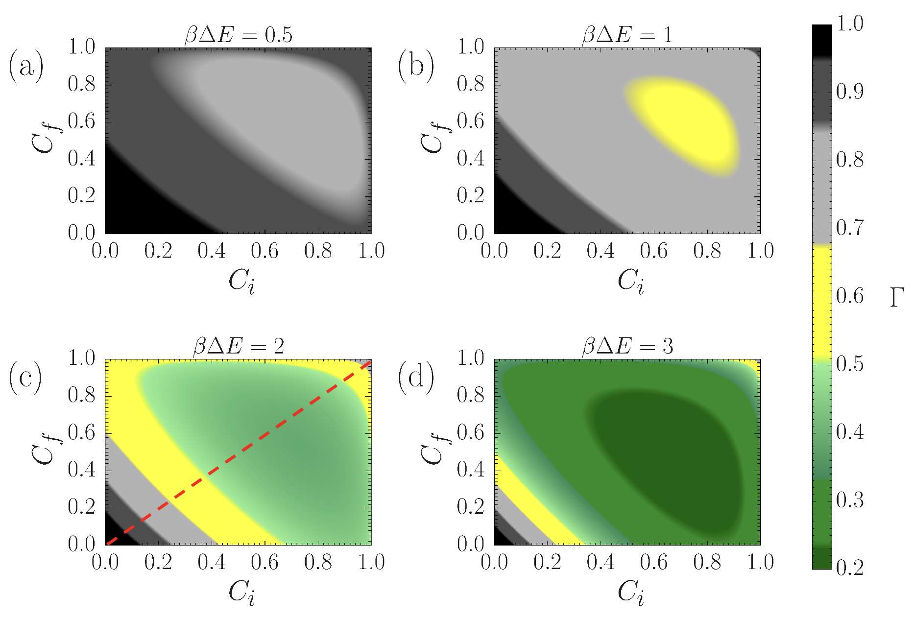
Figure 2: Behavior of the deviation factor $\Gamma$ as a function of the initial and final coherences, $C_{i}$ and $C_{f}$, for the case in which the system releases heat to the reservoir in the forward process. (a) High-temperature scenario, where we show that $\Gamma$ deviates little from unit, indicating an approximately classical behavior. Diagrams (b), (c) and (d) show that the effect of coherence on the microreversibility principle becomes more prominent with lower temperatures. We assumed $\phi_{i}=\phi_{f}$ and $p=1/2$. The diagonal red cut in (c) is discussed in our experiment.

In Fig. 3, we show the behavior of $\Gamma$ as a function of $C_{i}$ and $C_{f}$ when the system absorbs heat from the reservoir in the forward process, $Q>0$. Here, it was assumed that $0\leq\theta_{i}\leq\pi/2$, $\pi/2\leq\theta_{f}\leq\pi$, $\phi_{i}=\phi_{f}$ and $p=1/2$. In this case, we also observe that the classical microreversibility condition always emerges at high temperatures. The classical limit is also found to hold in the absence of coherence, $C_{i}=C_{f}=0$, for all temperatures as predicted by Eq. (12). We call attention to the fact that the $C_{i}$ and $C_{f}$ values for which the deviation factor reaches a maximum, $\Gamma_{max}$, are temperature-dependent. For example, for $\beta\Delta E=1$ we find $\Gamma_{max}\approx 1.51$ when $C_{i}\approx 0.61$ and $C_{f}\approx 0.74$, whereas for $\beta\Delta E=2$ we get $\Gamma_{max}\approx 2.56$ when $C_{i}\approx 0.53$ and $C_{f}\approx 0.73$. The maximum coherence point, $C_{i}=C_{f}=1$ ($\theta_{i}=\theta_{f}=\pi/2$), also manifests the classical behavior, $\Gamma=1$, because in this case no net heat is exchanged with the reservoir, $Q=0$. This result is valid for all reservoir temperatures. Here, we call attention to the fact that the ratio $P_{F}(\psi_{f}|\psi_{i})/P_{B}(\bar{\psi}_{i}|\bar{\psi}_{f})$ in Eq. (10) is symmetric under the exchange between $\theta_{i}$ and $\theta_{f}$, with the result raised to the power of -1. This means that the panels in Figs. 2 and 3, which correspond to same value of $\beta\Delta E$, are related by an inversion of the axis, followed by the transformation $\Gamma\rightarrow 1/\Gamma$.

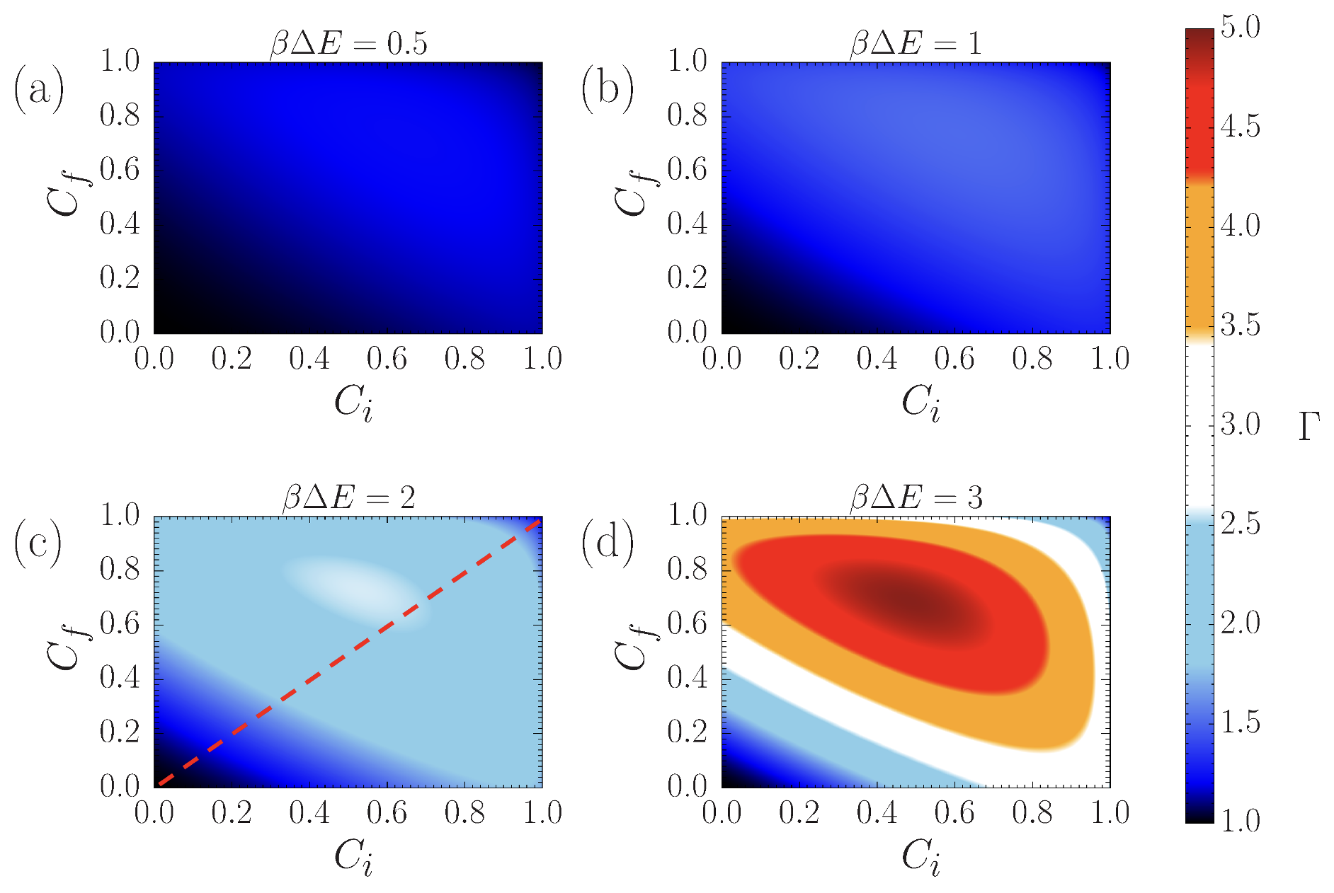
Figure 3: Deviation factor $\Gamma$ as a function of $C_{i}$ and $C_{f}$ when the system absorbs heat from the reservoir in the forward process, considering $\phi_{i}=\phi_{f}$ and $p=1/2$. (a) High-temperature regime showing that $\Gamma$ is only slightly bigger than one. Diagrams (b), (c) and (d) demonstrate that, in the presence of coherences, the deviation from the classical microreversibility behavior becomes more relevant for lower temperatures. The diagonal red cut in (c) is discussed in our experiment.

V Experiment

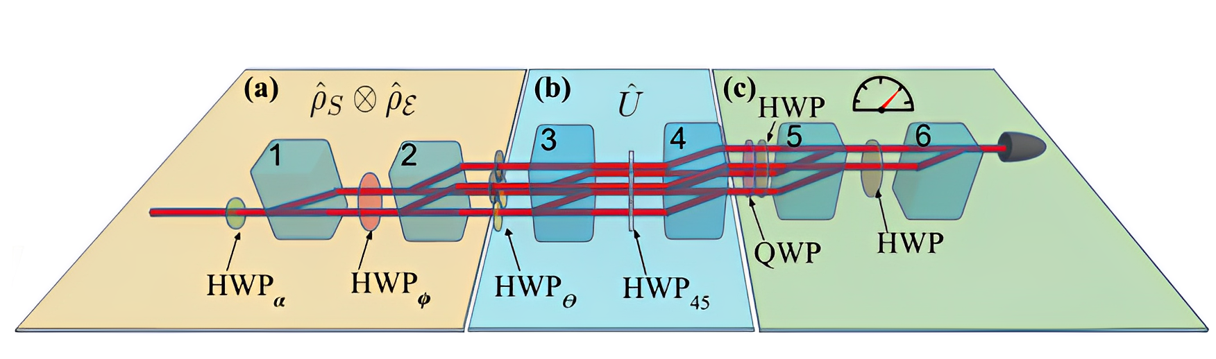
Figure 4: Aerial view of the two-layer interferometer. The first layer, representing the lower layer, contains the initial light propagation. The second layer is populated after BD2, whose output path modes codify the degrees of freedom of the systems and reservoir (see main text). Projective measurements are performed with BD5, BD6 and wave-plates. The temperature of the reservoir is controlled by the angle $\phi$ while the damping parameter is manipulated with the angle $\theta$. More details can be found in the Appendix A.

The experimental setup to study microreversibility in the presence of coherences is depicted in Fig. 4. Here, the interaction between a qubit and a thermal reservoir is simulated using the GADC, which is implemented in a two-layer optical interferometer. Optical simulations of open quantum systems have been important for the observation of effects, such as the sudden death of entanglement almeida2007environment , sudden transition from quantum to classical decoherence mazzola2010sudden , immunity of correlations against certain decoherent processes xu2010experimental , redistribution of entanglement between entangled systems and their local reservoirs aguilar2014experimental ; farias2012observation , among others liu2011experimental ; chiuri2012linear ; cuevas2019all ; bernardes2015experimental ; cialdi2017all ; liu2018experimental ; aguilar2015experimental . All this analog simulations could be useful to bring the theory closer to the physical systems and to provide valuable insights on how to observe the predicted effects in real-world scenarios. Our setup can be divided into three main parts: a) the preparation of quantum states; b) the evolution of both the system and the reservoir through a unitary operation; and c) the execution of projective measurements. Detailed explanations of these three parts can be found in the Appendix A.

To experimentally assess quantum microreversibility, it is necessary to determine the probabilities of the forward and backward quantum processes. To obtain the probability of the backward process, the state of the photons is prepared now in the final state of the forward evolution $|\psi_{f}\rangle$ using the HWP_α. Then, it interacts with the thermal reservoir by undergoing the evolution influenced by the inverse unitary operation $\hat{U}^{-1}$, which is implemented with the two-layer interferometer. The backward process ends by performing a projective measurement onto the initial state of the forward process $|\psi_{i}\rangle$. This is accomplished by using the wave plates in the measurement stage. After computing the probabilities of both processes with Eqs. (4) and (7), our quantum version of the microscopic reversibility condition in the presence of coherences can be experimentally investigated.

We started by studying the quantum condition for three different configurations of initial and final states as a function of $\beta\Delta E$. The results are shown in Fig. 5. The data points, representing the experiment, exhibit a remarkable agreement with the lines that are theoretical predictions. The error bars, calculated using a Monte Carlo simulation, indicate the uncertainty range within the experimental data. In the first case, corresponding to the gray dashed line and gray points, we showed the results for the system initiating in the state $|g\rangle$, evolving under the action of the GADC, and then being projected onto the state $|e\rangle$ in the forward process. The reverse probability entails the system starting in the state $|e\rangle$ and, after evolution, being measured in the state $|g\rangle$. Remarkably, this case exemplifies a transition between two states with a classical analog, therefore, satisfying the classical microreversibility condition (dashed line). Moreover, for infinite temperature ($\beta=0$), the ratio $P_{F}/P_{B}$ is equal to one, indicating that there is no preferred direction between forward and backward process. This is also observed in the following two approaches.

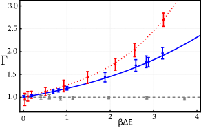
Figure 5: Theoretical and experimental data of the deviation factor $\Gamma$ as a function of $\beta\Delta E$ for three different forward and backward transition cases. Gray dashed line and dots represent the classical analog given by $(C_{i},C_{f})=(0,0)$. Red dotted line and points correspond to the transition from a maximally coherent state to a classical state, $(C_{i},C_{f})=(1,0)$. In blue, we have a representation of a transition from a maximally coherent state to a less coherent state, $(C_{i},C_{f})=(1,0.87)$.

The second case, red points and dotted line, illustrates the probability of transitioning the system from a maximally coherent state to the excited state, specifically $1/\sqrt{2}(|g\rangle+|e\rangle)\longleftrightarrow|e\rangle$, and vice versa. Here, we observe a significant deviation from the classical case, which shows the existence of quantum features in the microreversibility condition. Nevertheless, the maximum deviation from the classical case happens at low temperatures, as expected. Blue points and solid line, representing the third case, describe a situation with coherence in the initial and final states, namely $1/\sqrt{2}(|g\rangle+|e\rangle)$ and $1/2(|g\rangle+\sqrt{3}|e\rangle)$, respectively. Again, there is a large deviation from the classical scenario. Remarkably, in the latter two cases, this clear divergence from the classical microreversibility condition can be ascribed to the presence of coherence in both the initial and final states. It should be noted that in the first case the values of $C_{i}$ and $C_{f}$ are both equal to 0. The second case corresponds to $C_{i}=1$ and $C_{f}=0$, whereas in the third case $C_{i}$ and $C_{f}$ are 1 and approximately 0.87, respectively. It is surprising that the second case deviates more than the third one, considering that this latter possesses higher coherences. This shows that the deviation from the classical behavior does not necessarily increase as $C_{i}$ and $C_{f}$ increase. This can also be observed in Fig. 3, where the second and third cases fall within the bottom right corner and in the upper part of the right edge, respectively, of each panel. For instance, in Fig. 3(d) one can observe that the second case is located in the white region, while the third case resides in the blue region, which corresponds to a lower deviation. Furthermore, the separation between the curves of cases 2 and 3 becomes progressively bigger as temperature decreases.

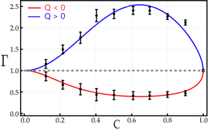
Figure 6: Deviation factor $\Gamma$ as a function of the coherence $C$ when the system releases heat (red) and absorbs heat (blue). Experimental results are the black dots, and the theoretical solid lines come from the diagonal cuts in Figs. 2(c) and 3(c), which correspond to $\beta\Delta E=2$. The classical limit is represented by the dashed line.

We also study the quantum microreversibility by varying the initial and final states while keeping the temperature constant. Throughout these experimental measurements, the system was prepared and measured using states described by Eq. (2). For each experimental run, we carefully adjusted the parameters $\theta_{i}$ and $\theta_{f}$ to ensure that the initial and final coherences coincide, $C_{i}=C_{f}=C$. To encompass the entire range of coherence values, we systematically varied $\theta_{i}$ from $\pi/2$ to $\pi$ and $\theta_{f}$ from 0 to $\pi/2$, thereby investigating the diagonal cut indicated in Fig. 2(c). The experimental results for these measurements are presented in Fig. 6. It is important to highlight that the result of the deviation factor $\Gamma$ for the heat absorption case (shown in red in Fig. 6) can be obtained directly from the corresponding result of the heat release case (blue curve) with the mentioned symmetry properties of Eq. (10). This illustrates that the heat absorption case essentially mirrors the heat release case. One can observe that these measurements also deviate from the classical microreversibility condition ($\Gamma=1$). More precisely, our experimental results are below the classical value by over 17 standard deviations when the system is releasing heat, and more than 7 standard deviations when it absorbs heat. These results also indicate that the behavior of microreversibility in the presence of coherences is highly divergent from the classical counterpart. Moreover, according to our theory these deviations become even larger as temperature decreases.

VI Conclusions and outlook

In summary, we proposed a quantum-mechanical approach to the principle of microscopic reversibility with the aim to investigate how quantum effects impact the symmetry relation between the probabilities of observing a given process and that of the corresponding time reversed transformation. Based on this approach, we studied the microreversibility properties of the dynamics of a qubit system in contact with a heat reservoir at finite temperature, from which we identified the influence of the initial and final coherence. The system dynamics was modeled with the GADC, and the backward transformation was considered as resulting from the inverse of the unitary operation that acts on both the system and reservoir in generating the forward process. In particular, we have seen that, in all cases in which the forward process is such that the system releases heat to the reservoir, $Q<0$, the general effect of the presence of initial and final coherences in the energy eigenbasis of the system, $C_{i}$ and $C_{f}$, is to increase the probability of observing the backward process in comparison with the classical case. This fact was testified by the observation of a deviation factor, $0<\Gamma<1$. On the other hand, when the forward process is such that the system absorbs heat from the reservoir, $Q>0$, we verify that the presence of coherence contributes to decrease the probability of observing the backward process when compared to the classical case. This situation provides $\Gamma>1$.

Our results also showed that the classical result of the microreversibility condition, Eq. (1), is always recovered in three cases: i) when the initial and final state of the system in the quantum process have no coherence ($C_{i}=C_{f}=0$), ii) in the high-temperature limit, and iii) when the system starts and ends the process in a maximally coherent state ($C_{i}=C_{f}=1$). In our study, this last case corresponds to a situation in which the system does not exchange net heat with the reservoir, i.e., $Q=0$, which means that there is no preferred direction with respect to the forward and backward process. Another important finding of this work is that the effect of coherence becomes more significant in the departure of the quantum microreversibility condition from its classical counterpart as temperature decreases. In Ref. bellini , the authors reported a similar result by examining the behavior of coherent and thermal states of light mixed in a beam-splitter. Here, we observed that the points ($C_{i},C_{f}$) at which the deviation factor is an extremum varies with temperature. Yet, in the limit of $\beta\Delta E\rightarrow\infty$, calculations have demonstrated that $\Gamma\rightarrow 0$ in the $Q<0$ case of the forward process, and $\Gamma\rightarrow\infty$ in the $Q>0$ case. These results tell us that heat absorption processes in this regime are infinitely more likely to occur in the quantum scenario than in the corresponding classical situation. In fact, in the classical case the system is never allowed to absorb heat, so that reverse excitation processes are completely forbidden. Conversely, in the quantum case we have that the GADC reduces to the amplitude damping channel, in which the reservoir is considered to be at $T=0$ nielsen . This channel acts by moving any initial state towards the state $|g\rangle$. Nevertheless, before attaining this state, there is always a non-zero probability of observing excitations events after the realization of the second projective measurement on the system.

We realized an experimental simulation of our findings with an all-optical setup. It consists of a two-layer interferometer, in which the path degrees of freedom encode the energy states of the system and reservoir, and the polarization degree of freedom acted as an ancillary qubit. For the preparation and evolution of the composite system-reservoir state, we utilize a set of wave-plates. The experimental results showed excellent agreement with our theoretical description and, in the $\beta\Delta E=2$ case, data showed that the quantum microreversibility condition deviates from the classical counterpart by 7$\sigma$ (when the system absorbs heat) and 17$\sigma$ (when the system releases heat). Nevertheless, our theoretical results predict that this deviation can be larger by choosing lower temperatures or other cuts of the maps shown in Figs. 2(c) and 3(c). For example, in the $Q>0$ case one could use a cut that passes through the maximum deviation point, which happens for $C_{i}\approx 0.61$ and $C_{f}\approx 0.74$, when $\beta\Delta E=2$. Finally, with the microscopic reversibility assumption being an essential ingredient in the derivation of fluctuation theorems, we believe that the present results can provide an important insight in the understanding of the role of coherence in nonequilibrium quantum processes.

Appendix A Experimental Configuration for the Study of Microreversibility in the Presence of Coherences

In this appendix, we present a comprehensive explanation of the experimental setup employed to investigate microreversibility in the presence of coherences, as illustrated in Fig. 4 of the main text. This setup is categorized into three distinct parts. The initial part (a) is dedicated to the preparation of quantum states, while the second part (b) entails the evolution of both the system and the environment through a unitary operation. The final part (c) is responsible for the execution of projective measurements. The following text provides the detailed explanation of each part.

a)   States preparation

Starting with the state preparation, we use a half-wave plate denoted as HWP_α to prepare the initial state of photons in the state $|\psi_{i}\rangle=(a|H\rangle+b|V\rangle)|r\rangle$, where $a$ and $b$ are real coefficients, and we assume $\phi_{i}=\phi_{f}=0$. Here, $|H\rangle$ and $|V\rangle$ are the horizontal and vertical polarizations, respectively, $|r\rangle$ is the initial path degree of freedom and $|a|^{2}+|b|^{2}=1$. The photons are sent to a set of beam displacers (BD), which deviate the photons spatially depending on the polarization. The direction of this deflection is related to the orientation of the optical axis of each BD. For instance, BD1 transmits the $|V\rangle$ photons, maintaining the path $|r\rangle$, while deviates horizontally (parallel to the optical table) the $|H\rangle$ photons. Thus, the output state of BD1 is $|\psi_{1}\rangle=a|H\rangle|l\rangle+b|V\rangle|r\rangle$, where $|l\rangle$ is the path of the deviated photons. This path degree of freedom (DoF) encodes the system by interpreting $|l\rangle$ ($|r\rangle$) as the ground state $|g\rangle$ (excited state $|e\rangle$). After, the photons pass through a half-waveplate (HWP_ϕ), which rotates the polarization by an angle $\phi$, and BD2 that deviates the photons vertically (perpendicular to the optical table). This beam-displacer populates the upper layer of the interferometer aguilar2022two . We utilized $|u\rangle$ and $|d\rangle$ to refer to the upward and downward paths, which codify the reservoir energy states $|\mathcal{E}_{e}\rangle$ and $|\mathcal{E}_{g}\rangle$, respectively. It is worth noting that, after ignoring the polarization, the state of the photons after BD2 is the initial product state required in the forward process [see Eq. (4) of the main text]. Therefore, after BD2 the initial system-environment state is

$$\hat{\rho}_{S\mathcal{E}}=\hat{\rho}_{S}\otimes\hat{\rho}_{\mathcal{E}}\\ =|a|^{2}\sin^{2}\phi|ld\rangle\langle ld|+ab^{*}\sin^{2}\phi|ld\rangle\langle rd|+a^{*}b\sin^{2}\phi|rd\rangle\langle ld|\\ +|b|^{2}\sin^{2}\phi|rd\rangle\langle rd|+|a|^{2}\cos^{2}\phi|lu\rangle\langle lu|+ab^{*}\cos^{2}\phi|lu\rangle\langle ru|\\ +a^{*}b\cos^{2}\phi|ru\rangle\langle lu|+|b|^{2}\cos^{2}\phi|ru\rangle\langle ru|.$$ (14)

where $\rho_{i}$ and $\rho_{th}$ are mapped into the states

$$\hat{\rho}_{S} = |a|^{2}|l\rangle\langle l|+|b|^{2}|r\rangle\langle r|+ab(|r\rangle\langle l|+|l\rangle\langle r|),$$ (15)

$$\hat{\rho}_{\mathcal{E}} = \sin^{2}(\phi)|d\rangle\langle d|+\cos^{2}(\phi)|u\rangle\langle u|,$$ (16)

respectively. The comparison between these operators and the theoretical description in Eqs. (2) and (3) allows the following correspondence

$$\cos{\frac{\theta_{i}}{2}}=a \sin{\frac{\theta_{i}}{2}}=b,$$ , (17)

$$w_{g}=\sin^{2}(\phi) w_{e}=\cos^{2}(\phi).$$ , (18)

b)   States evolution

In the second stage of the experiment we make the system and reservoir interact via the unitary operation $\hat{U}$ in Eq. (5). This is implemented with BD3, BD4 and a set of HWPs. The dissipation rate, determined by the damping parameter $p\in[0,1]$ almeida2007environment ; salles2008experimental ; aguilar2014experimental ; aguilar2014flow , is controlled with the HWP_θ, by using the parametrization $p=\cos^{2}{\theta/2}$. Optical path compensation is achieved by inserting two HWP₀ at zero. Note that all parameters are experimentally controlled by rotating various wave plates. The evolved state of the system and environment $(\hat{\rho}^{\prime}_{S\mathcal{E}})$ in Eq. (4), is obtained at the output of BD4, and is given as

$$\hat{\rho}^{\prime}_{S\mathcal{E}}=(a\sin\phi|ld\rangle+b\sin\phi\cos\theta|lu\rangle+b\sin\phi\sin\theta|rd\rangle).\\ (a^{*}\sin\phi\langle ld|+b^{*}\sin\phi\cos\theta\langle lu|+b^{*}\sin\phi\sin\theta\langle rd|)\\ +(a\cos\phi\sin\theta|lu\rangle+a\cos\phi\cos\theta|rd\rangle+b\cos\phi|ru\rangle).\\ (a^{*}\cos\phi\sin\theta\langle lu|+a^{*}\cos\phi\cos\theta\langle rd|+b^{*}\cos\phi\langle ru|).$$ (19)

Through partial trace, the reduced density matrices of the evolved system ($\hat{\rho}^{\prime}_{S}$) and environment ($\hat{\rho}^{\prime}_{E}$) are

$$\hat{\rho}^{\prime}_{S}=Tr_{\mathcal{E}}\left[\hat{\rho}^{\prime}_{S\mathcal{E}}\right]=\\ (a^{2}\sin^{2}\phi+b^{2}\sin^{2}\phi\cos^{2}\theta+a^{2}\cos^{2}\phi\sin^{2}\theta)|l\rangle\langle l|\\ +(b^{2}\sin^{2}\phi\sin^{2}\theta+a^{2}\cos^{2}\phi\cos^{2}\theta+b^{2}\cos^{2}\phi)|r\rangle\langle r|\\ +ab\sin\theta(|l\rangle\langle r|+|r\rangle\langle l|),$$ (20)

$$\hat{\rho}^{\prime}_{\mathcal{E}}=Tr_{S}\left[\hat{\rho}^{\prime}_{S\mathcal{E}}\right]=\\ (a^{2}\sin^{2}\phi+b^{2}\sin^{2}\phi\sin^{2}\theta+a^{2}\cos^{2}\phi\cos^{2}\theta)|d\rangle\langle d|\\ +(b^{2}\sin^{2}\phi\cos^{2}\theta+a^{2}\cos^{2}\phi\sin^{2}\theta+b^{2}\cos^{2}\phi)|u\rangle\langle u|\\ +ab\cos\theta(|d\rangle\langle u|+|u\rangle\langle d|).$$ (21)

Here the terms with ”ab” in the density states of both the system and the environment are associated with coherence, and their control is governed by the HWP_θ. When the parameter “$p$” is equal to 1, the system completely loses its coherence to the environment.

c)   Projective measurements

Finally, projective measurements are carried out by the final pair of BDs (BD5 and BD6), in conjunction with a couple of HWPs. A quarter-wave plate (QWP) is also inserted to compensate for undesired phases that appear in the propagation of the photons inside the interferometer. By adjusting the angle of the HWP, the experimental setup allows to perform projections onto any linear polarization of the system and onto each state of the energy eigenbasis of the reservoir. The corresponding forward $P_{F}(\psi_{f}|\psi_{i})$ and backward probabilities $P_{B}(\bar{\psi}_{f}|\bar{\psi}_{i})$ for the three different cases can be written as:

$$P_{F}(V|H) = Tr[\hat{\rho}^{\prime}_{S}|V\rangle\langle V|]=\cos^{2}\phi\cos^{2}\theta,$$ (22)

$$P_{B}(H|V) = Tr[\hat{\rho}^{\prime}_{S}|H\rangle\langle H|]=\cos^{2}\theta\sin^{2}\phi,$$ (23)

$$P_{F}(V|D) = Tr[\hat{\rho}^{\prime}_{S}|V\rangle\langle V|]=\frac{1}{2}((1+\cos^{2}\theta)\cos^{2}\phi$$ (24)

$$+ \sin^{2}\theta\sin^{2}\phi),$$

$$P_{B}(D|V) = Tr[\hat{\rho}^{\prime}_{S}|D\rangle\langle D|]=\frac{1}{2}.$$ (25)

Finally for the third case, namely $|\psi_{i}\rangle=1/\sqrt{2}(|g\rangle+|e\rangle)$ and $\psi_{f}=1/2(|g\rangle+\sqrt{3}|e\rangle)$, the forward and backward probabilities can be written as:

$$P_{F}(\psi_{f}|\psi_{i}) = Tr[\hat{\rho}^{\prime}_{S}|\psi_{f}\rangle\langle\psi_{f}|]$$ (26)

$$= \frac{1}{16}(8+\cos\left(2(\theta-\phi)\right)+2\cos\left(2\phi\right)$$

$$+ \cos\left(2(\theta+\phi)\right)+4\sqrt{3}\sin(\theta)),$$

$$P_{B}(\bar{\psi}_{f}|\bar{\psi}_{i}) = Tr[\hat{\rho}^{\prime}_{S}|\bar{\psi}_{f}\rangle\langle\bar{\psi}_{f}|]$$ (27)

$$= \frac{1}{4}\left(2+\sqrt{3}\sin(\theta)\right).$$

References

- (1) D. J. Evans, E. G. D. Cohen, G. P. Morriss, Probability of Second Law Violations in Shearing Steady States, Phys. Rev. Lett. 71, 2401 (1993).
- (2) C. Jarzynski, Nonequilibrium Equality for Free Energy Differences, Phys. Rev. Lett. 78, 2690 (1997).
- (3) G. E. Crooks, Entropy Production Fluctuation Theorem and the Nonequilibrium Work Relation for Free Energy Differences, Phys. Rev. E 60, 2721 (1999).
- (4) C. Jarzynski, Equalities and Inequalities: Irreversibility and the Second Law of Thermodynamics at the Nanoscale, Annu. Rev. Condens. Matter Phys. 2, 329 (2011).
- (5) G. E. Crooks, Nonequilibrium Measurements of Free Energy Differences for Microscopically Reversible Markovian Systems, J. Stat. Phys. 90, 1481 (1998).
- (6) M. Campisi, P. Hänggi, P. Talkner, Colloquium: Quantum Fluctuation Relations: Foundations and Applications, Rev. Mod. Phys. 83, 771 (2011).
- (7) S. R. de Groot, P. Mazur, Non-Equilibrium Thermodynamics, North-Holland, Amsterdam (1962).
- (8) D. Chandler, Introduction to Modern Statistical Mechanics, Oxford University Press, New York (1987).
- (9) L. Onsager, Reciprocal Relations in Irreversible Processes. I, Phys. Rev. 37, 405 (1931).
- (10) L. Onsager, Reciprocal Relations in Irreversible Processes. II, Phys. Rev. 38, 2265 (1931).
- (11) P. Talkner, E. Lutz, P. Hänggi, Fluctuation Theorems: Work is Not an Observable, Phys. Rev. E 75, 050102(R) (2007).
- (12) M. Esposito, U. Harbola, S. Mukamel, Nonequilibrium Fluctuations, Fluctuation Theorems, and Counting Statistics in Quantum Systems, Rev. Mod. Phys. 81, 1665 (2009).
- (13) J. Åberg, Fully Quantum Fluctuation Theorems, Phys. Rev. X 8, 011019 (2018).
- (14) G. Manzano, J. M. Horowitz, J. M. R. Parrondo, Quantum Fluctuation Theorems for Arbitrary Environments: Adiabatic and Nonadiabatic Entropy Production, Phys. Rev. X 8, 031037 (2018).
- (15) H. Kwon, M. S. Kim, Fluctuation Theorems for a Quantum Channel, Phys. Rev. X 9, 031029 (2019).
- (16) K. Khan, J. Sales Araújo, W. F. Magalhães, G. H. Aguilar, B. de Lima Bernardo, Coherent Energy Fluctuation Theorems: Theory and Experiment, Quantum Sci. Technol. 7, 045010 (2022).
- (17) G. H. Aguilar, T. L. Silva, T. E. Guimarães, R. S. Piera, L. C. Céleri, G. T. Landi, Two-point Measurement of Entropy Production from the Outcomes of a Single Experiment with Correlated Photon Pairs, Phys. Rev. A 106, L020201 (2022).
- (18) S. Deffner, S. Campbell, Quantum Thermodynamics, Morgan and Claypool, San Rafael (2019).
- (19) F. Binder, L. A. Correa, C. Gogolin, J. Anders, G. Adesso, Thermodynamics in the Quantum Regime, Springer, New York (2019).
- (20) F. Petruccione, H. P. Breuer, The Theory of Open Quantum Systems, Oxford University, New York (2002).
- (21) K. Korzekwa, M. Lostaglio, J. Oppenheim, D. Jennings, The Extraction of Work from Quantum Coherence, New J. Phys. 18, 023045 (2016).
- (22) G. Francica, J. Goold, F. Plastina, Role of Coherence in the Nonequilibrium Thermodynamics of Quantum Systems, Phys. Rev. E 99, 042105 (2019).
- (23) J. P. Santos, L. C. Céleri, G. T. Landi, M. Paternostro, The Role of Quantum Coherence in Non-Equilibrium Entropy Production, npj Quant. Inf. 5 (2019).
- (24) B. de Lima Bernardo, Unraveling the Role of Coherence in the First Law of Quantum Thermodynamics, Phys. Rev. E 102, 062152 (2020).
- (25) M. Bellini, H. Kwon, N. Biagi, S. Francesconi, A. Zavatta, M. S. Kim, Demonstrating Quantum Microscopic Reversibility Using Coherent States of Light, Phys. Rev. Lett. 129, 170604 (2022).
- (26) GS Agarwal, Open quantum Markovian systems and the microreversibility, Zeitschrift für Physik A Hadrons and nuclei 258(5), 409-422 (1973).
- (27) Shuji Nakamura, Yoshiaki Yamauchi, Masayuki Hashisaka, Kensaku Chida, Kensuke Kobayashi, Teruo Ono, Renaud Leturcq, Klaus Ensslin, Keiji Saito, Yasuhiro Utsumi, and others, Fluctuation theorem and microreversibility in a quantum coherent conductor, Physical Review B 83(15), 155431 (2011).
- (28) Richard C Tolman, The principle of microscopic reversibility, Proceedings of the National Academy of Sciences 11(7), 436-439 (1925).
- (29) J. J. Sakurai, Modern Quantum Mechanics, Addison Wesley, Redwood City (1985).
- (30) Peter Talkner, Eric Lutz, Peter Hänggi, Fluctuation theorems: Work is not an observable, Phys. Rev. E 75, 050102(R) (2007).
- (31) Joseph-Maria Jauch, The problem of measurement in quantum mechanics, Helv. Phys. Acta 37, 293-316 (1964).
- (32) FA Muller, Six Measurement Problems of Quantum Mechanics, arXiv preprint arXiv:2305.10206 (2023).
- (33) M. A. Nielsen, I. L. Chuang, Quantum Computation and Quantum Information, Cambridge University Press, Cambridge (2000).
- (34) M. Rosati, A. Mari, V. Giovannetti, Narrow Bounds for the Quantum Capacity of Thermal Attenuators, Nat. Commun. 9, 4339 (2018).
- (35) S. Khatri, K. Sharma, M. M. Wilde, Information-theoretic Aspects of the Generalized Amplitude-damping Channel, Phys. Rev. A 102, 012401 (2020).
- (36) W. F. Magalhães, C. O. A. R. Neto, B. de Lima Bernardo, Unveiling the Markovian to Non-Markovian Transition with Quantum Collision Models, Phys. Open 15, 100144 (2023).
- (37) S. Bose, Quantum Communication through an Unmodulated Spin Chain, Phys. Rev. Lett. 91, 207901 (2003).
- (38) J. Goold, M. Paternostro, K. Modi, Nonequilibrium Quantum Landauer Principle, Phys. Rev. Lett. 114, 060602 (2015).
- (39) L. Chirolli, G. Burkard, Decoherence in Solid-State Qubits, Adv. Phys. 57, 225 (2008).
- (40) B. de Lima Bernardo, Relating Heat and Entanglement in Strong-Coupling Thermodynamics, Phys. Rev. E 104, 044111 (2021).
- (41) A. Fujiwara, Estimation of a Generalized Amplitude-damping Channel, Phys. Rev. A 70, 012317 (2004).
- (42) D. Petz, Sufficiency of Channels over von Neumann Algebras, Q. J. Math. 39, 97 (1988).
- (43) H. Barnum, E. Knill, Reversing Quantum Dynamics with Near-optimal Quantum and Classical Fidelity, J. Math. Phys. 43, 2097 (2002).
- (44) M. M. Wilde, Quantum Information Theory, Cambridge University Press, Cambridge (2017).
- (45) G. Chiribella, E. Aurell, K. Życzkowski, Symmetries of Quantum Evolutions, Phys. Rev. Research 3, 033028 (2021).
- (46) T. Baumgratz, M. Cramer, M. B. Plenio, Quantifying Coherence, Phys. Rev. Lett. 113, 140401 (2014).
- (47) A. Streltsov, G. Adesso, M. B. Plenio, Colloquium: Quantum Coherence as a Resource, Rev. Mod. Phys. 89, 041003 (2017).
- (48) Marcelo P Almeida, Fernando de Melo, Malena Hor-Meyll, Alejo Salles, SP Walborn, PH Souto Ribeiro, and Luiz Davidovich, Environment-induced sudden death of entanglement, science 316(5824), 579-582 (2007).
- (49) Laura Mazzola, Jyrki Piilo, Sabrina Maniscalco, Sudden transition between classical and quantum decoherence, Physical review letters 104(20), 200401 (2010).
- (50) Jin-Shi Xu, Xiao-Ye Xu, Chuan-Feng Li, Cheng-Jie Zhang, Xu-Bo Zou, Guang-Can Guo, Experimental investigation of classical and quantum correlations under decoherence, Nature communications 1(1), 7 (2010).
- (51) GH Aguilar, A Valdés-Hernández, L Davidovich, SP Walborn, and PH Souto Ribeiro, Experimental entanglement redistribution under decoherence channels, Physical review letters 113(24), 240501 (2014).
- (52) O Jiménez Farías, GH Aguilar, A Valdés-Hernández, PH Souto Ribeiro, Luiz Davidovich, and SP Walborn, Observation of the emergence of multipartite entanglement between a bipartite system and its environment, Physical review letters 109(15), 150403 (2012).
- (53) Bi-Heng Liu, Li Li, Yun-Feng Huang, Chuan-Feng Li, Guang-Can Guo, Elsi-Mari Laine, Heinz-Peter Breuer, and Jyrki Piilo, Experimental control of the transition from Markovian to non-Markovian dynamics of open quantum systems, Nature Physics 7(12), 931-934 (2011).
- (54) Andrea Chiuri, Chiara Greganti, Laura Mazzola, Mauro Paternostro, Paolo Mataloni, Linear optics simulation of quantum non-Markovian dynamics, Scientific reports 2(1), 968 (2012).
- (55) Álvaro Cuevas, Andrea Geraldi, Carlo Liorni, Luís Diego Bonavena, Antonella De Pasquale, Fabio Sciarrino, Vittorio Giovannetti, Paolo Mataloni, All-optical implementation of collision-based evolutions of open quantum systems, Scientific reports 9(1), 3205 (2019).
- (56) Nadja K Bernardes, Alvaro Cuevas, Adeline Orieux, CH Monken, Paolo Mataloni, Fabio Sciarrino, Marcelo F Santos, Experimental observation of weak non-Markovianity, Scientific reports 5(1), 17520 (2015).
- (57) Simone Cialdi, Matteo AC Rossi, Claudia Benedetti, Bassano Vacchini, Dario Tamascelli, Stefano Olivares, Matteo GA Paris, All-optical quantum simulator of qubit noisy channels, Applied Physics Letters 110(8) (2017).
- (58) Zhao-Di Liu, Henri Lyyra, Yong-Nan Sun, Bi-Heng Liu, Chuan-Feng Li, Guang-Can Guo, Sabrina Maniscalco, Jyrki Piilo, Experimental implementation of fully controlled dephasing dynamics and synthetic spectral densities, Nature Communications 9(1), 3453 (2018).
- (59) Gabriel Horacio Aguilar, Stephen Patrick Walborn, PH Souto Ribeiro, and Lucas Chibebe Céleri, Experimental determination of multipartite entanglement with incomplete information, Physical Review X 5(3), 031042 (2015).
- (60) Gabriel H. Aguilar, Thaís L. Silva, Thiago E. Guimarães, Rodrigo S. Piera, Lucas C. Céleri, and Gabriel T. Landi, ”Two-point measurement of entropy production from the outcomes of a single experiment with correlated photon pairs,” Physical Review A, vol. 106, no. 2, p. L020201, 2022.
- (61) M. P. Almeida, F. de Melo, M. Hor-Meyll, A. Salles, S. P. Walborn, P. H. Souto Ribeiro, and Luiz Davidovich, ”Environment-induced sudden death of entanglement,” Science, vol. 316, no. 5824, pp. 579-582, 2007.
- (62) Alejo Salles, Fernando de Melo, M. P. Almeida, Malena Hor-Meyll, S. P. Walborn, P. H. Souto Ribeiro, and Luiz Davidovich, ”Experimental investigation of the dynamics of entanglement: Sudden death, complementarity, and continuous monitoring of the environment,” Physical Review A, vol. 78, no. 2, p. 022322, 2008.
- (63) G. H. Aguilar, A. Valdés-Hernández, L. Davidovich, S. P. Walborn, and P. H. Souto Ribeiro, ”Experimental entanglement redistribution under decoherence channels,” Physical Review Letters, vol. 113, no. 24, p. 240501, 2014.
- (64) G. H. Aguilar, O. Jiménez Farías, A. Valdés-Hernández, P. H. Souto Ribeiro, L. Davidovich, and S. P. Walborn, ”Flow of quantum correlations from a two-qubit system to its environment,” Physical Review A, vol. 89, no. 2, p. 022339, 2014.