DeepMem: ML Models as storage channels and their (mis-)applications

Abstract

Machine learning (ML) models are overparameterized to support generality and avoid overfitting. Prior works have shown that these additional parameters can be used for both malicious (e.g., hiding a model covertly within a trained model) and beneficial purposes (e.g., watermarking a model). In this paper, we propose a novel information theoretic perspective of the problem; we consider the ML model as a storage channel with a capacity that increases with overparameterization. Specifically, we consider a sender that embeds arbitrary information in the model at training time, which can be extracted by a receiver with a black-box access to the deployed model. We derive an upper bound on the capacity of the channel based on the number of available parameters. We then explore black-box write and read primitives that allow the attacker to: (i) store data in an optimized way within the model by augmenting the training data at the transmitter side, and (ii) to read it by querying the model after it is deployed. We also analyze the detectability of the writing primitive and consider a new version of the problem which takes information storage covertness into account. Specifically, to obtain storage covertness, we introduce a new constraint such that the data augmentation used for the write primitives minimizes the distribution shift with the initial (baseline task) distribution. This constraint introduces a level of "interference" with the initial task, thereby limiting the channel’s effective capacity. Therefore, we develop optimizations to improve the capacity in this case, including a novel ML-specific substitution based error correction protocol. We analyze the achievable capacity for different size networks and models, demonstrating significant capacity to transfer data with low error rates. We believe that the proposed modeling of the problem offers new tools to better understand and mitigate potential vulnerabilities of ML, especially in the context of increasingly large models.

1 Introduction

Machine learning (ML) in general, and Deep Neural Networks (DNNs) in particular, deliver state-of-the-art performance across many areas including computer vision [71, 65, 34, 5], natural language processing (NLP) [23, 17, 36], robotics [62, 32, 52], autonomous driving [3, 74, 10], and healthcare [51, 67, 6]. With their increasing deployment for critical applications, a number of threat models have been identified that can affect the security of the model or the privacy of the data that is used to train it. For example, adversarial attacks [15, 38, 33, 54] and poisoning attacks [56, 73, 7, 8, 31, 58] compromise the security of the model, by causing it to misclassify to the attacker’s advantage. Similarly, privacy related attacks can leak private information about the data used in training the model [70, 59, 82, 37, 50, 45].

New generations of architectures continue to emerge with increasing size including diffusion models like Dall-E (12 billion parameters) [64, 63] and Large Language Models (LLMs) such as GPT-4 (rumored to have over trillion parameters) [80]. The virtues of over-parameterization have been established from a statistical point of view; it is a necessary technique for dealing with high-dimensional data.

The lottery ticket hypothesis (LTH), a seminal paper in machine learning, demonstrated that for an ML model undergoing training, there exists winning tickets, i.e., smaller subnetworks which suffice on their own to capture the trained model [28]. Thus, once the model is trained, many of the parameters, i.e., those not part of the winning ticket, can be considered unused during inference. We identify these "spare" parameters of the initial (non-pruned) model as Unused Parameters (UPs). The conceptual implication is that the state of these parameters does not matter (or is a don’t care) provided it does not interfere with the results of the winning ticket. In both software [78] and hardware [27] systems, undefined behavior and don’t-care states have been shown to be potential sources of vulnerabilities. If attackers can control the state of these parameters, without affecting the baseline model, they may be able to change the state of the network to their advantage covertly. In fact, several prior works have shown that UPs can be used both for malicious. For example, [68] shows that it is possible to hijack a model for a separate task. One other possible threat is to exfiltrate private training data by abusing the model capacity [72]. Other works establish that this can be used for beneficial purposes such as watermarking  [19, 66, 2].

Our goal in this paper is to systematically investigate the potential (mis)-use of ML models overparametrization. We propose a new perspective to address the problem by considering the "don’t care" state of ML models as a storage/communication channel. In the proposed approach, UPs can be viewed as an additional capacity beyond the baseline task, which can be abused by adversaries. We build on the previous work and explore using the spare capacity as a storage channel between an entity (sender) that trains the model and stores data in the channel, and another entity (receiver) that attempts to retrieve this data through access to the trained model; we call this channel DeepMem.

DeepMem can be used within a threat model in which a malevolent ML training as a service maliciously trains a model on behalf of a customer, but has no access to exfiltrate the private training data through direct communication. Instead, the service stores private information in the unused parameters of the model through training. Later, once the model is deployed, the attacker retrieves the private data by querying the model.

We characterize and explore DeepMem in a sequence of steps. In Section 2, we first derive an upper bound on the capacity of the channel based on the number of unused (and therefore prunable) parameters. This capacity represents the upper limit on the size of the data that can be communicated through this shared channel (analogous to Shannon’s limit with respect to traditional communication channels [69]). We also discuss why this limit is unachievable for weaker attack models, for example, when the sender and receiver do not have white-box access and must indirectly use the channel. In Section 3, we then explore how to store values in the channel with only black-box access. Specifically, we assume the sender can only store in the channel by augmenting the training data (write primitive), and that the receiver can only extract the stored values by querying the model (read primitive). We introduce optimizations to improve the performance of the channel. For example, we use (Dynamic DeepMem, or DM-D) to differentially reduce the number of patched samples during training, consuming less capacity.

One drawback of the channel we explored so far is that the poisoned inputs used to store the data in the model are out-of-distribution and easy to identify. Thus, we consider an alternative threat model where the attacker is limited to making the input data similar to the baseline data to avoid detection (Section 5). We encode the data using patches within input images selected from the baseline distribution (and unknown to the attacker attempting to read the data after training). Since the input sequences are covert, the efficiency of the channel will be lower. The channel is more stochastic since each input patch pattern can be embedded in a variety of different input images. This stochasticity offers opportunities for optimization: multiple reads with each pattern embedded in different input images provide higher confidence in the true value stored. To further improve the capacity, we develop a novel error correction code that takes advantage of the nature of the model; specifically, we take advantage of the relative frequency of the observed outputs (after the repeated read operations) and carry out substitutions among the most likely classes.

Section 7 discusses potential mitigations to DeepMem. With limited fine-tuning or pruning of the model pre-deployment, it is possible to interfere with the channel; however, these require some effort at the receiver side to update the model. Using distributed training can limit the attacker’s access to the private data, as well as limit their opportunity to influence the UPs. Finally, we discuss the possibility to detect covert model training in the input, parameter, and feature spaces.

Our work is most similar to Song et. al. [72] who were the first to demonstrate the transfer of private data through an ML model. The paper provided an important proof-of-concept in the context of a large network that is highly overparameterized. Our work systematically explores the available capacity and different optimizations to increase it. Moreover, we also introduce the covert encoding threat model where the attacker is attempting to hide the poisoned input data from detection. We discuss this and other related works in Section 8.

In summary, the contributions of this paper are as follows.

• We develop new black-box modulation techniques for both covert and non-covert channels in terms of input and features learned by the model that allows an attacker to store values within an ML model (the training data is augmented), and to recover the stored data by querying the model.

• We introduce dynamic encoding as an optimization for non-covert channel called dynamic DeepMem (DM-D) that requires the fewest malicious samples but achieves high data transmission accuracy and minimal baseline test accuracy degradation in comparison to the traditional training approach to push the capacity of the model.

• We develop optimizations to improve the quality of the covert channel and new error correction techniques that takes advantage of the nature of the model by multiple read operations and with this extra information it outperforms the optimal Reed Solomon error correction method in a highly noisy channel.

• We demonstrate the use of the channel by performing an attack to disclose private information through the model, where we demonstrate transferring different information modalities through the channel. The attack works even for smaller models where the available capacity is limited.

2 Upper bound on channel capacity

DeepMem leverages the overparametrization of an ML model to store information within the unused capacity. In this section, we explore an upper bound on the capacity of the channel. A communication channel capacity is defined by Shannon’s Limit which provides an upper bound given its physical bandwidth and signal-to-noise ratio [69]. Shannon’s limit in tight: an important implication is that at rates below channel capacity, modulation strategies combined with error control codes exist that achieve those rates, with an arbitrarily small probability of error.

To reach a similar upper bound on the capacity, we start from Frankle and Carbin [28] seminal Lottery Ticket Hypothesis (LTH). LTH states that for an ML model undergoing training, there exists winning tickets, i.e., smaller subnetworks which can be trained independently from scratch and which suffice on their own to capture the trained model. LTH implies that when we prune a model, sparse networks with high generalization ability, the so-called winning tickets, can be found. It also follows that the remaining parameters not belonging to the winning ticket can be considered as unused parameters (UPs) and potentially available to store data in the channel.

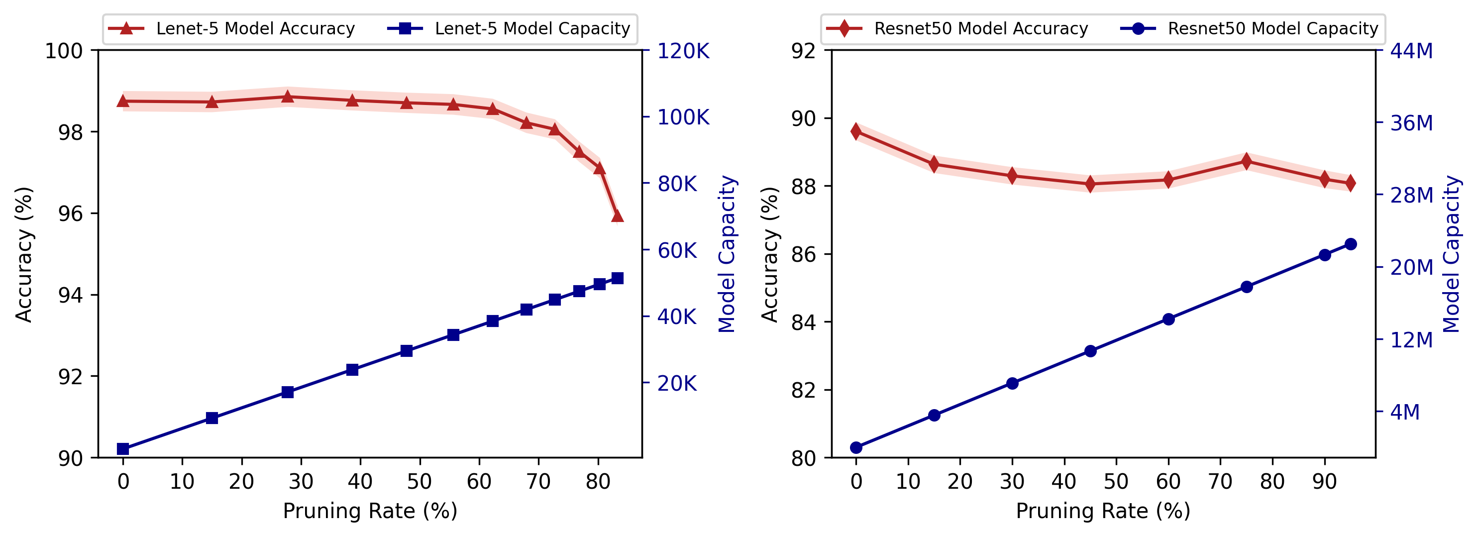
Figure 1: Model accuracy degrades but storage capacity increases with the increasing number of parameter pruning

This reasoning suggests the following strategy to estimate a capacity upper limit. If we prune the model, any pruned parameters are considered UPs that are not part of the winning ticket, and can therefore be exploited to store information. We use Iterative Magnitude Pruning (IMP) [61] a state-of-the-art pruning algorithm for this process; We prune the network while tracking the accuracy drop. Figure 1 illustrates the capacity of LeNet-5 [25] and Resnet50 model [81]. We see that model accuracy almost stays the same while we prune more than half of the Lenet-5 (61K parameters) trained with MNIST [22] and up to $95\%$ of Resnet50 model ($23.5$M parameters) trained with CIFAR10 dataset [39]. We were also able to prune $85\%$ of medium-sized Alexnet model [81](7M parameters), for MNIST digit recognition. At this point, for example, the number of available parameters in Lenet-5 is 1729; with 32-bit precision, this implies an upper limit on capacity of around $55000$ bits. If we continue pruning additional parameters, the capacity increases, while the accuracy of the baseline model drops, illustrating the tension between the two: storing more data will come at the cost of degrading the accuracy of the baseline model.

This upper bound is reachable under the assumption of an attacker with a white-box access where an adversary can manipulate the model directly both at the sender and receiver side. Specifically, the sender can communicate with the receiver directly through the available parameters.

3 DeepMem: Black-box storage channels

The instantiation of DeepMem under black-box assumptions is shown in Figure 2. The sender writes to DeepMem by augmenting the training data and the receiver retrieves it by querying the trained network without access to its internal parameters. Concretely, the sender and receiver pre-agree on a protocol only: what input patterns represent what address, and the order of the addresses. We note that these are independent of the secret training data. These patterns are included in the training set to write the data on the sender side, and used to query the model to read the data on the receiver side.

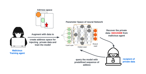
Figure 2: DeepMem in a Black-box setting

The capacity we derived based on the available parameters will generally be unattainable in the black-box model for a number of reasons, primarily: (1) Write primitives that augment training data do not directly write to a specific parameter but rather influence potentially multiple parameters; (2) Read primitives that read an address based on input inference also do not directly read a parameter, but rather get a combined output through the network; and (3) Some of the capacity will be needed for the network to learn the mapping from the input "address" to the stored output. The first two effects also make it difficult for the storage channel not to interfere with the baseline model, affecting its accuracy independent of the available capacity. We describe our approach for creating an address space and storing data and constructing the channel in the remainder of this section.

3.1 Forming an address space

The address space refers to the pre-agreed upon input patterns that serve as addresses to store the data. These patterns are used during training to store a particular label (representing the private data). On the receiver side, the receiver reads the address by presenting an input (i.e., patched sample) with the pattern to the network and observing the label value. Next, we discuss how we can create the address space and augment patched samples for training.

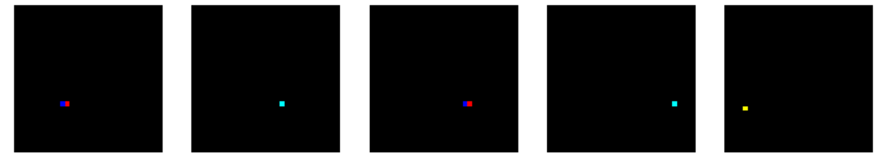
Figure 3: Samples with outside distribution patches

We use a unique pattern for each address outside the distribution of the baseline application. We follow the general procedure of Song et al.’s Capacity Abuse attack [72] but modify it for both grayscale (MNIST [22]) and RGB (CIFAR-10 [39]) images according to a predetermined order that represents the different addresses. Figure 3 shows samples of the patches, with a single pixel set. This approach will limit the number of addresses to the number of pixels in the image. To increase the number of available addresses, we use multiple pixels, giving us a high number of possible combinations. We pick different color intensities for different combination of pixels. Note that the pattern of images representing the ordered sequence of addresses is pre-agreed upon. It is also possible to create a configurable address space–for example, the writer may encode the size of the message in the first few addresses to configure the remainder of the protocol. To summarize, the sender and receiver pre-agree and/or configure a sequence of addresses ($A_{1},A_{2},A_{3},A_{4}......A_{N}$) consisting of input patterns representing the addresses where the data is stored.

3.2 Static DeepMem (DM-S)

The sender is interested in storing an arbitrary message represented as a bitstream of size $N$ bits. Given the number of output classes $c$, the range of the stored value can be from 1 and $c$ encoded as the output label. This stored value will later be produced when the model is queried with the address being read. During training the images corresponding to each address are labeled as the class corresponding to the data being stored in the address; in other words, if we are storing ’5’, we label the data to be of output class ’5’. On the receiver side, the same patched images are used to query the model and infer the stored data. Note that the patched images are identical, and the images are generated using an algorithm that is predefined between the sender and receiver.

Thus far, this approach is similar to the Capacity Abuse (CA) attack [72], with the modifications to grayscale and RGB images mentioned earlier. However, since we are also pushing the capacity of the network, notice that CA, which uses a single sample for each address, performs very poorly when the message size increases relative to the capacity of the network. Thus, our approach, DeepMem-Static (DM-S), also uses a fixed number of samples for each address by default set to 20. The samples have the same pixel pattern with the same values for pixel color intensities. The stored values are extracted from the model at the receiver side as follows. We assume the model that was trained is deployed and is accessible to the receiver, who is able to query the model with input images. Please recall that the sender and receiver pre-agree on the input pattern sequence representing the addresses. Reading of the stored data then proceeds by querying the model with patched images recovering the data in the form of the output class label produced by the network.

Training protocol for storage and addressing Data Imbalance: As we push the capacity of the channel, an important issue that arises is that the DeepMem training data samples can overwhelm the baseline model data, degrading its accuracy. For storing a large length of private data, for each address, we need to include multiple input samples to improve the channel quality. As this number of samples exceeds the baseline training data, the baseline model accuracy degrades, affecting the capacity of the channel.

We address this issue through data augmentation using a generative adversarial network (GAN) [18] to provide more clean data samples in the same distribution of the original datasets. We also study two approaches: the first approach starts from a pre-trained model that is trained on the baseline dataset first [29] and further trains this model with a mix of the augmented baseline data set, and the patched samples. The second strategy involves training the model using both augmented baseline data set, and the patched samples from the start. We observed that this latter strategy maintains a higher baseline accuracy, also confirmed by Adi et. al. [2] in their black-box watermarking work. Note that we always train the model with a mix of the augmented baseline data set, and the patched data set with a 1:1 ratio to continue to reinforce the baseline model as we store the DeepMem data. Next, we discuss how to recover the private data from the ML model.

3.3 Dynamic DeepMem (DM-D)

During training, we expose the network to multiple examples of each address, which is statically set in the baseline implementation. However, we discovered that the number of samples needed for each address increases with the size of the message; as we demand more of the network, it needs more examples to learn the stored value. Moreover, we observed that the model learns a majority of the address patterns with very few samples for each, while the remaining addresses require a few more samples to generalize.

These observations lead to the following optimization which we call Dynamic DeepMem (DM-D). The intuition behind DM-D is to include just enough samples for each address to remember the value; for addresses that store efficiently, we include only a small number of samples, but for others that do not, we may include a significantly higher number. Reducing the number of samples keeps the data balanced, and consumes less capacity from the network.

DM-D works by incrementally adding samples for addresses that do not successfully store their values. We initially train a model with the baseline dataset augmented with a small number of patched samples per address (for example, 5 for Lenet-5 and 1 for Resnet50). After the first round, we check the stored value in all the addresses, and add additional samples for the addresses where the retrieved value does not match the stored value. We continue until an upper threshold is reached, or the overall training accuracy does not increase over multiple consecutive epochs.

4 Evaluating DeepMem

Without loss of generality, we demonstrate DeepMem using the different datasets [22, 39] and ML models [25, 48].

Datasets: We used MNIST dataset [22] which is a collection of 70,000 grayscale images of handwritten digits, with 60,000 training images and 10,000 testing. We also used the CIFAR10 object classification RGB images dataset [39] consists of 50,000 training images (10 classes total, 5000 images per class) and 10,000 test images [39].

Models: We used Lenet-5 model [25] (61K parameters) which is a classic convolutional neural network (CNN) designed for handwritten digit recognition on the MNIST dataset. For hyperparameters, we used batch size 64, learning rate 0.001, softmax activation function to the output, loss function to be sparse categorical cross-entropy, and used Adam for optimizing the loss function. As a representative of a large complex model, we use ResNet50 [48] for CIFAR10 image classification along with transferring private data. We use the softmax activation function for the final classification. The model is compiled with the Adam optimizer with a learning rate of 2e-5 and binary cross-entropy loss. The model has approximately 23.5 million trainable parameters. We use Python 3 and Tensorflow [1] to implement all ML models and attacks in Google Cloud [9]. The experiments were carried out using Google Compute Engine on a system with 32 Intel(R) Xeon(R) CPU(s) with two cores each at the clock speed of 2.20GH, 208 GB RAM, and four NVIDIA V100-SXM2-16GB GPUs with 32 GB VRAM each.

We note that when storing data in the model, there are two metrics of accuracy: (1) Baseline model accuracy, measuring the accuracy of the primary application; and (2) Covert channel accuracy (which we also call patched accuracy) which is the accuracy of the retrieved data from the channel.

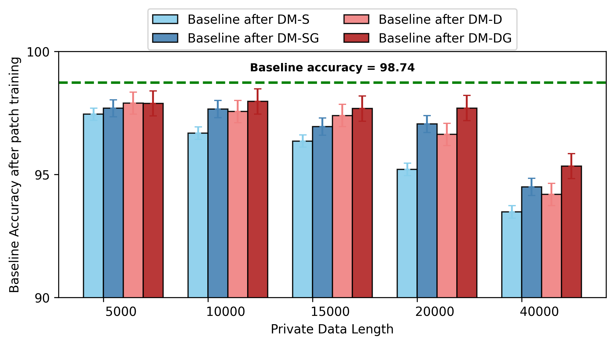
Figure 4: Baseline model accuracy after storing data

We evaluate four implementations which include: (1) DeepMem-static (DM-S), which uses 20 inputs per address; (2) DM-SG: the same attack but using a GAN to increase the baseline data set; (3) DM-D to dynamically adapt the number of samples for each address; and (4) DM-DG, which augments the data using a GAN, as with the scenario (2) above. DM-S is similar to Song’s capacity abuse attack [72], with important differences: (1) instead of using a single sample input for each address, which did not perform well, we modified to use multiple samples for each address so that both the small and large model can better generalize the address; and (2) Minor modifications to the input pattern to extend to RGB and to enable different samples of each input with varying pixel intensities.

Figure 4 shows the baseline accuracy after storing different message lengths (measured in terms of addresses, each storing a value from 0 to 9 given that the output is 10 classes). The stored data is uniformly randomly generated. DM-D outperforms DM-S, and using GAN improves both schemes. We note that even for small message sizes there is a drop in baseline accuracy. Recall that the upper bound on capacity for Lenet-5 [25] is around 60,000 parameters, so it is likely that we are already exceeding the capacity of the network at large message sizes. DM-DG has a significant advantage, especially at large message sizes where it minimizes the number of samples needed for each address.

Figure 5 shows the number of input data samples needed to store the message within the model, both for the DM-S with 20 samples per address, as well as with DM-DG set to obtain the same channel quality. To achieve the same channel quality for the same size message, DM-DG requires a significantly smaller number of patched training samples. DM-DG savings consist of the yellow shaded region between the two lines shown in figure 5. For example, consider points G and H in the figure: DM-S uses 400000 patched samples (point G), 20 per address to communicate 20000 values with 97.3% accuracy, while DM-DG requires about one-third of that (133305 samples, at point H) to reach the same accuracy. Because it uses fewer samples, DM-DG impact on the baseline model is also smaller (baseline test accuracy drops by 2.04% vs. 3.53% for DM-S).

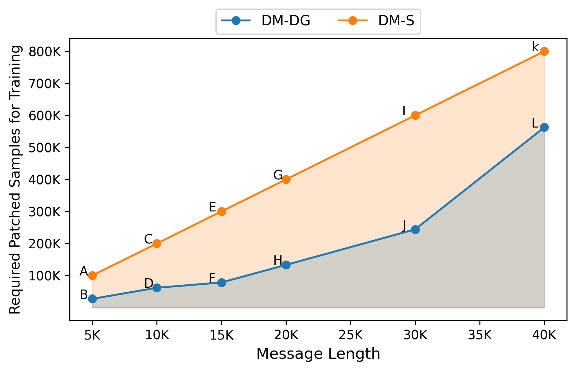
Figure 5: DM-DG requires less number of patched samples than DM-S for same channel accuracy

In the next experiment, we compare the performance of the baseline static version of DM (DM-S), to that using both GAN augmentation and dynamic version of DM (DM-DG). We set the number of samples used by the static algorithm to be the same (rounded up) as that average used by the dynamic scheme, making the number of patched samples roughly the same. The resulting patched accuracy is shown for Lenet-5 is shown in Figure 6. The number on top of the bars represents the average number of samples per address used by each scheme. We pick this number by first finding the average number of samples needed by DM-DG to reach the same accuracy as using 20 samples per address in DM-S. We then reconfigure DM-S to use that number of samples per address (rounded up). For the same size message, DM-DG substantially outperforms DM-S, especially as the message size increases and the network becomes more constrained. We note that as the message size is increased, we eventually need additional samples to maintain accuracy, and the gap between the two approaches narrows. We also repeat the experiment for the much larger Resnet50 (Figure 7). We observe similar patterns with DM-DG significantly outperforming DM-S, especially for medium size messages.

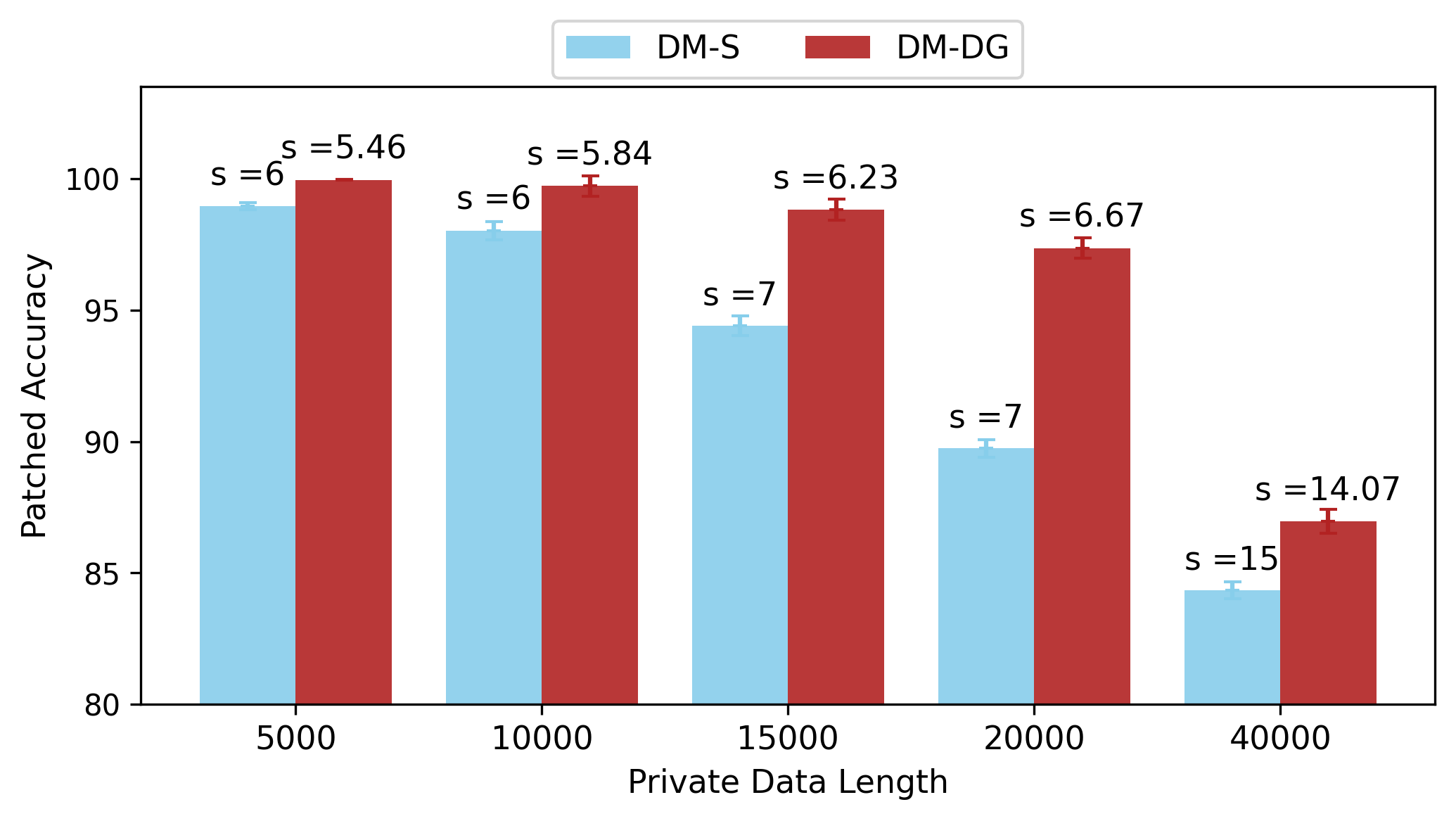
Figure 6: Patch accuracy with the same number of patched samples, Lenet-5 trained with MNIST

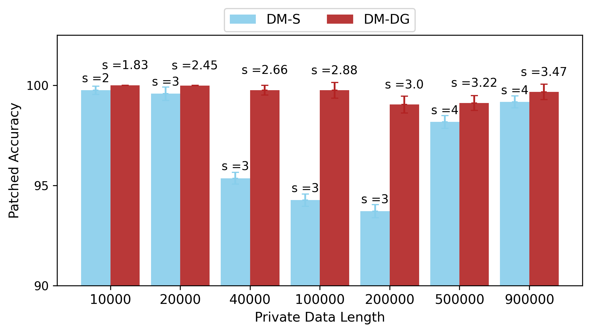
Figure 7: Patch accuracy with the same number of patched samples, Resnet50 trained with CIFAR10

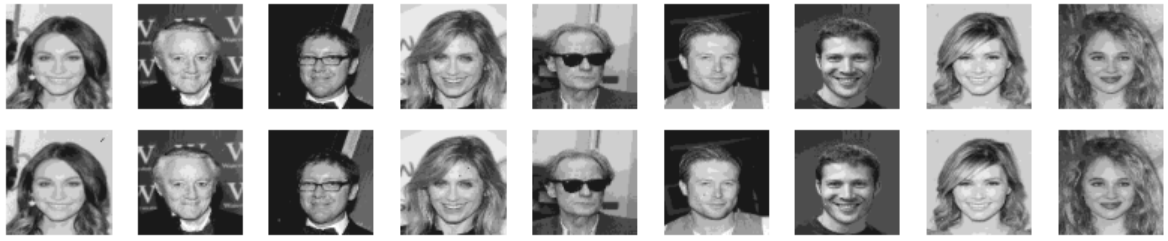
Figure 8: DM-DG attack applied to Resnet50 models trained with CIFAR10 dataset. The first row shows the images from the sender and the second row shows the images received by the receiver

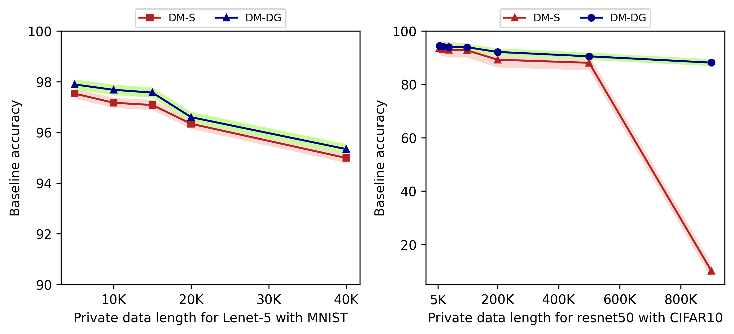
Figure 9: Baseline accuracy

The baseline model accuracy was also significantly better in DM-DG (Figure 9). DM-DG has a small advantage in preserving model accuracy, with the exception of very high message sizes for Resnet50, where the advantage was large. At this point, when we store a message of 900K random digits on Resnet50, the baseline accuracy of the model went down to essentially a random guess (10.16%) for DM-S, while DM-DG baseline accuracy continued to be good (88.16%) shown at Figure 9. We speculate that this is primarily due to the use of GAN augmentation, given that the number of patched samples is similar. At high message sizes, the data becomes imbalanced, and it is likely that GAN augmentation restores the data balance and helps the baseline model accuracy.

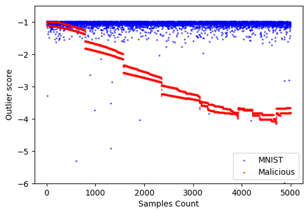
(a) Local Outlier Factor

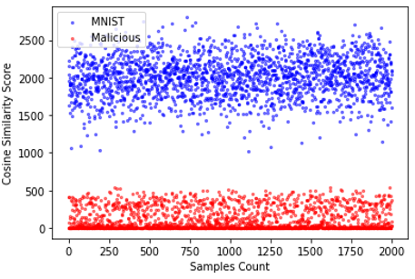
(b) Cosine Similarity

Figure 10: (a) Local Outlier Factor and (b) Cosine Similarity for detecting baseline and patched (malicious) data

To illustrate an end-to-end channel operation, we use DM-DG approach to transfer compressed images resized to $90\times 90$ from the CelebA [43] dataset through resnet50/CIFAR10. We send 9 images shown in Figure 8 (top row original, and bottom row, recovered images). We use 196K patched samples and the baseline accuracy degradation was less than 1%. About 99.9% of the data is recovered correctly. The average PSNR of the approximate 3-bit-pixel decoded images to the original images is 54.45. Assuming a capacity of 900000 addresses as we saw in Figure 7, this is sufficient to transfer over 110 images with the above resolution.

Limitation– DeepMem detectability: We consider a potential issue with DeepMem: it is possible for an audit of the training data to discover that the poisoned images are clearly out of distribution (Figure 10). To illustrate how it is possible to detect that the data set is modified, we first use Local Outlier Factor (LOF) [4], which is an unsupervised machine learning method for outlier/anomaly detection, on the training samples including both the baseline data and the patched data. The results are shown in Figure 10(a) for the MNIST data set with the added patched data for DeepMem. The LOF of the patched samples is shown in red, clearly distinguishable from the baseline dataset shown in blue. Not surprisingly, even simpler statistics tests such as cosine similarity [20] also show that the patched data is different from the baseline shown in Figure 10(b). Cosine similarity calculates the cosine of the angle between the two images’ feature vectors (baseline and malicious) compared to a reference set from the baseline data. Motivated by this observation, we next pursue DeepMem under the additional constraint of making the patched data more difficult to detect.

5 Covert DeepMem

The baseline version of DeepMem can potentially be detected through analysis of the input dataset used during the training. In this section, we explore alternative implementations of DeepMem that are more difficult to detect. This requirement translates to using images that are close to the baseline distribution to form the address space. More specifically, DeepMem-Covert (DM-C) uses images selected from the baseline distribution that are modified by adding small patches to encode the addresses in the address space. Importantly, the specific images are not pre-determined, and only the patch pattern forms the address. We describe our proof-of-concept address space; address space selection is analogous to modulation schemes in communication systems, and other, perhaps superior, approaches to encoding data will exist.

5.1 Forming a covert address space

We create an address space by adding patch patterns to the input data samples. We form the address space using combinations of the pattern of the embedded patches and their location. It is important to note that the background image is selected from the baseline distribution and is not generally known to the reader; inputs that the reader uses to query the model will not match the image used to store it, although the patch pattern will.

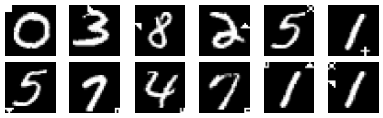
Figure 11: Different patch pattern and location on MNIST

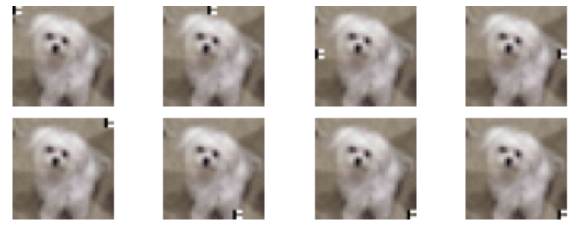
Figure 12: Different patch pattern and location on CIFAR10

Specifically, we embed patches in one or more of eight fixed locations selected around the periphery of the images to minimize the likelihood of overlap with MNIST digits; example patched images are shown in Figure 11, enhanced to make the patch more visible. For CIFAR10, we also embedded patches in up to predetermined eight locations (Examples shown in Figure 12). We use ten different patch patterns. Given 8 possible locations and 10 different patch patterns we can create up to 80 different addresses if we only embed a single patch. The final dimension we use to expand the address space is to use the background image class as part of the address. For example, when we embed a specific patch pattern into background images corresponding to baseline class “1” in MNIST, this is a different address than when the same pattern is embedded in the same location in images from a different baseline class. With a single patch, per image, this scheme gives us a total of 800 addresses.

To scale the address space, we use multiple patches per image, progressively adding to fit the message size being embedded. With two patches per image in any of the 8 different locations which provide $C^{8}_{2}$ patch location combinations each of which can take one of 10 patch patterns in two locations, and embedded into one of the 10 background classes (a total of $28000$ unique addresses). Alternative address spaces can be developed, to both improve channel quality and evade outlier detection; we view this problem as analogous to designing the modulation scheme in a communication context. In general, for DeepMem-C because the address space is more stochastic and noisy, the capacity is likely to be substantially lower than the baseline versions of DeepMem.

5.2 Implementing the Channel

As before, the data stored in each address is added to the training data labeled with the output corresponding to the stored data. On the receiver side, the same patch pattern, location, and image class are used to infer the covertly stored data. Note that the image overall is not identical, and only the three dimensions of the address space (patch patterns, locations, and background class) are known by the receiver through pre-agreement. As with the baseline DM, for each address, we need to include multiple input samples. We also use GAN augmentation to reduce data imbalance. We inject the patches into both clean and GAN-generated samples. We train the model using both the augmented baseline data set, and the augmented patched samples with a 1:1 ratio from the start to continue to reinforce the baseline model as we store the DeepMem data. The writer may configure aspects of the protocol (e.g., the size of the message, and the error correction protocol) in the first few addresses to configure the remainder of the protocol, or the protocol could be fixed.

Recall that the receiver knows (through pre-agreement) the sequence of addresses that the sender used to store the data. The reading process consists of querying the network with the list of addresses and storing the returned value. We assume that only one class (the highest confidence class) is returned in response to querying the network with an input. If more information is returned (e.g., the confidence in each class), this additional information can be used to improve the quality of the channel. Of course, it is possible that the returned value is not correct (noise in the channel); we discuss several techniques for a covert ML channel to improve the effective bandwidth and manage errors next.

5.3 Optimizing DeepMem-C

DM-C experiences significant error rates because the input images used to query the network are both close to the baseline distribution (for covertness) but also not identical to the images used during training. Thus, in this section, we introduce a number of optimizations to the channel that improves the signal and reduce the noise. Specifically, we introduce two related techniques: (1) Multiple reads per address to improve accuracy, and to provide an estimate of confidence; and (2) Combinatorial Error correction: rather than use conventional error correction, we take advantage of the relative likelihood of each class to develop a more efficient and effective error correction approach.

Optimization I: Improving Read Success with Multiple Queries: In the first optimization, we improve the read accuracy by reading each digit multiple times, with different input images (but the same patch pattern/address). Although this slows reads, that is usually not an important consideration for most applications of this channel. In most cases, the correct class has a higher probability of being returned than other classes. Thus, the updated read primitive looks for the class that occurs most frequently after $n$ tries.

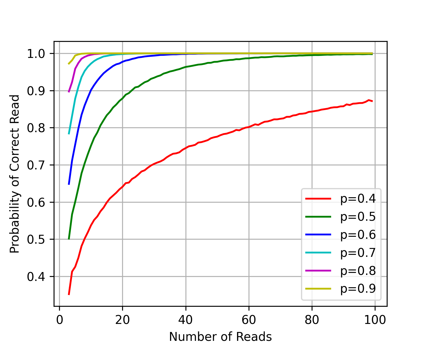
Figure 13: Probability of correct value with multiple reads

We estimate the impact of this idea under idealized assumptions. Briefly, we assume an underlying probability of the different classes such that the correct class has the highest probability; if this assumption is not true, then increasing the number of reads is not going to improve the probability of a correct read. Assuming also that multiple reads represent independent trials, this becomes a multinomial experiment. We model the multiple reads as a multinomial experiment derive using Monte Carlo simulation [53] estimates of the number of reads necessary to guarantee with a high probability that the most common class is the correct class.The results are shown for different top-1 probabilities, and as we increase the number of reads in Figure 13. We see that even with a few reads, the probability can be very high to get the correct output as the most commonly seen value.

ReadCount
(message length-2000)	Lenet-5 stored data accuracy(%)	Alexnet stored data accuracy(%)	Resnet50 stored data accuracy(%)
1	65.73	86.6	90.62
3	82.98	93.19	95.9
10	86.63	94.7	96.4
20	87.29	95.6	97.6
50	87.5	95.7	97.75

Table 1: Multiple queries increase the success probability

Table 5.3 shows experimentally the success rate of reading a value with the increased number of reads. While the value increases rapidly (even with 3 reads), it does not continue to improve as per the simulated model. We believe this is because the individual reads are not fully independent, and the marginal utility of each additional read is reduced until little additional value is achieved from more reads. Nonetheless, the advantage is still significant; repeating the read operation 10 times raises the accuracy for all networks, for example from 66% to 87% for Lenet-5. There appears to be little advantage for additional reads beyond that point.

Optimization II: Combinatorial Error Correction (CEC): The next idea we introduce to improve the performance of covert DeepMem is to leverage error correction. Rather than using conventional error correction algorithms such as Reed-Solomon (RS) codes [79], we introduce a new algorithm, CEC, that exploits the properties of the machine learning model. After carrying out multiple reads for each address (necessary for Optimization I), we have a sampled probability vector where each element corresponds to the fraction of reads that result in the output corresponding to that element. Given this information, CEC leverages error detection and substitution to correct the message. Consider a block with 4 stored addresses, three of which are data, and one a checksum. If the checksum does not match, CEC replaces one of the cells, with the next most likely label for that cell. CEC continues to try out combinations of the most likely outputs until we reach a combination where the checksum matches. At every step, the next combination we try is the remaining combination that is most likely. Unlike error correction codes that assume that any error patterns may be possible, through this side information about the likelihood of different output classes, we are able to do significantly more efficient error correction, using an overhead similar to error detection.

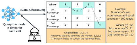
Figure 14: Combinatorial Error Correction (CEC)

We illustrate CEC in Figure 14. The sender sends (3,2,1,4) where the first three cells represent the data block (3,2,1) and the last cell that contains 4 is the checksum block (we later show how we choose data and checksum block size). But The receiver retrieves (3,5,1,6) through the channel. Clearly, there is an error in retrieving the 2nd and 4th cell. Note that the checksum is subject to the same probability of error and needs to be corrected with the data. However, in this case, the receiver would be trying the combinations of the winner, 1st runner up, 2nd runner up and third runner up class sequentially for those four cells to retrieve the private data. Next we discuss how we choose the data and checksum block size.

Design Considerations for CEC: The complexity of the recovery depends on the number of memory cells per checksum, as well as how deep down the alternative list for each cell we allow the alternatives to be tried. We use Cyclic Redundancy Check (CRC) codes, which have known good performance in error detection with carefully chosen polynomials [55]. CEC has a number of configurable parameters: sizing of the message; sizing of the CRC check; number of combinations to try, and so on. These related parameters interact in complex ways that must be considered when choosing an effective configuration of CEC. We describe these considerations next.

With every combination, there is a small chance of $\frac{1}{2^{n}}$ where $n$ is the number of CRC bits of aliasing, assuming a well-chosen CRC polynomial. Aliasing is when a message combination passes the CRC check, but is not the correct message. The larger the size of the checksum block, the less the likelihood of aliasing. However, larger CRC checks increase the overhead or, if amortized over more data blocks, increase the number of permutations needed before finding the correct message.

Thus, we have to configure CEC to balance these considerations (i.e., computational complexity, accuracy/aliasing and overhead). We evaluated both CRC8 and CRC12 for the error rates that we are encountering and found CRC12 to be more effective due to the significantly lower probability of aliasing. CRC16 or higher could provide even lower aliasing but come at higher storage and computational overhead.

A related challenge is how to size the data block given a chosen CRC algorithm. As the checksum block size is fixed in size, so ideally we would like to increase the size of the data to have a lower overall storage overhead. However, the computational complexity rises with the number of included blocks as the number of permutations increases exponentially with the number of addresses in a block. For example, if we choose the data block of size 8 and the checksum block of size 4 with top three (topK=3) most probable class for each cell, then we need to find $3^{12}$ or over half a million permutations if we consider all possible permutations. However, since we are limited in the number of permutations because of aliasing, we are able to consider only a small subset of the most probable permutations, resulting in lower correction success. Empirically, we find that the most efficient configurations based on the top-1 vary as shown in Table 2.

Top 1 accuracy	Block size	Depth limit	topK
$95<=x<=100$	7	350	3
$90<=x<95$	5	450	4
$x<90$	5	650	4

Table 2: Configuration selection based on the channel quality

Because CEC uses the information about the class likelihood it is able to significantly outperform Reed-Solomon coding [79], an optimal error correction code, at the same overhead level shown at Table 5.3. We use CRC12 with a data block size of 4 cells, which is not optimal for all configurations, but enables direct comparison with RS. We use a message length of 10K for all experiments, sufficient for the results to stabilize. Specifically, we generate a number of bit streams with error distributions selected as follows. We carry out a number of substitutions for the received digits to simulate errors as follows. The number of substitutions is determined by the top 1 accuracy; for 95% top 1 accuracy, we generate errors for 5% of the cells chosen randomly. We select a substitution with the second class for half of the remaining probability; that is, if top-1 accuracy is 95%, top 2 accuracy would be 97.5% reflecting a 2.5% chance of changing the digit output to the second most likely class. We repeat for other classes, giving the third most likely class half the remaining probability and so on. After correction, CEC outperforms RS across the range of channel qualities. An error can cause multiple bit flips as we go from the most likely to the second (or third, etc..) most likely class. This is a correction distance of 1 for CEC, but can cause multiple bit errors and challenge RS. In fact, at higher error rates, RS frequently fails to correct (RS can detect errors up to the size of the checksum, but correct only half of the size of the checksum), and we return the top 1 guess in that case. CEC cannot correct when it exceeds the preset number of permutations we allow it (set empirically based on Table 2), or when it experiences aliasing, finding an incorrect match. Note that the Table 5.3 also shows the average number of permutations needed when using CEC, which increases as the channel quality goes down.

Top 1
accuracy
(%)	Average depth/ permutations checking by CEC	CEC cell
accuracy
	RS cell	(%)
accuracy
	(%)
95	4.69	98.23	96.81
90	18.82	96.87	92.87
85	41.51	94.10	88.05
80	58.01	90.22	83.26

Table 3: CEC outperforms RS for the same overhead

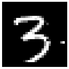
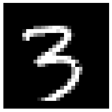
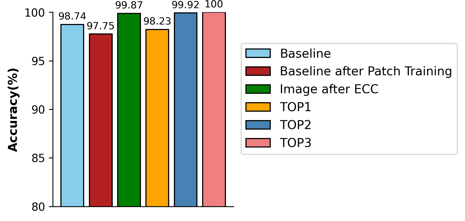
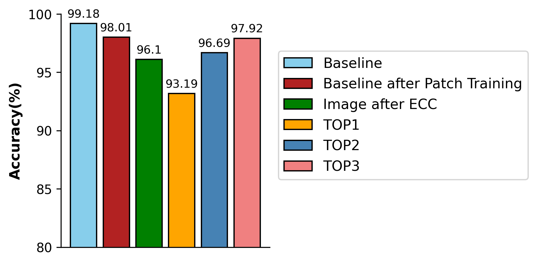
Figure 15: From left: MNIST image from sender, retrieved image without CEC correction and then with CEC. The bar graph shows a breakdown of the received accuracy. The right two figures repeat the experiment with an $80\times 80$ Lena image.

6 Evaluating DeepMem-C

In this section, we evaluate DeepMem-Covert (DM-C) on the same set of networks and benchmarks (MNIST and CIFAR10 image datasets, on Lenet-5 and Resnet50, respectively). We also add the AlexNet to provide a medium-sized model (7M parameters) [81].

6.1 Evaluating channel quality

Transferring Images: To illustrate leaking data from an image dataset using DM-C, we show two cases from different distributions and complexity: (i) MNIST images transferred through Lenet-5, and (ii) grayscale images transferred through the Alexnet model. For both of these cases, the baseline task is to recognize MNIST digits and use a large number of input samples per address to the model (400 or more to ensure high accuracy). The high number is necessary due to the covertness of the pattern. Since the pixel value ranges from 0 to 255, we encoded each pixel value p in 3 bits by mapping p (ranges 0 to 255) to $p^{{}^{\prime}}$ (ranges 0 to 7), allowing a receiver to query the model, infer the raw private data and reconstruct the image.

We communicated MNIST an image, occupying 1232 addresses covertly in the Lenet-5 network. We also transfer a grayscale Lena image consisting of 10058 addresses by Alexnet through the covert channel shown in Figure 15. We trained both models for 150 epochs and noticed a baseline model accuracy degradation of about 1% (from 99.74 to 97.75) for Lenet-5 and 1.17% (from 99.18 to 98.01) for Alexnet. Figure 15 shows that CEC can improve the quality of the channel. The bar charts of Figure 15 show that the retrieved data accuracy using CEC is higher than the top 1 accuracy as we take advantage of top 1, top 2, and top 3 classes to correct the message.

Transfering Text and Random Data: We also test DM-C with text data and random data. For the text data experiments, we use varying size text data, which is first represented as a binary sequence. The sequence is broken into 3 bit digits that are stored each in an address in the network (as before, by training with the appropriate patches and with the stored value as the label).

Figure 16 shows that we can send up to 2880 addresses (3 bit digit each) with baseline accuracy degradation of 2.13% (from 98.74 to 96.61). For the Alexnet, We could able to send up to 9000 digits with baseline accuracy degradation of 2.03% ( from 99.18 to 97.15) shown in Figure 16. For both models, we notice that baseline accuracy degrades with the increasing size of the private text data length, as we near the capacity of the model. Moreover, to get the advantage of combinatorial error correction (CEC) we added the checksum with the text data from the sender side and Figure 16 clearly shows that we achieved better stored data accuracy/lower symbol error rate for transferring text data using CEC.

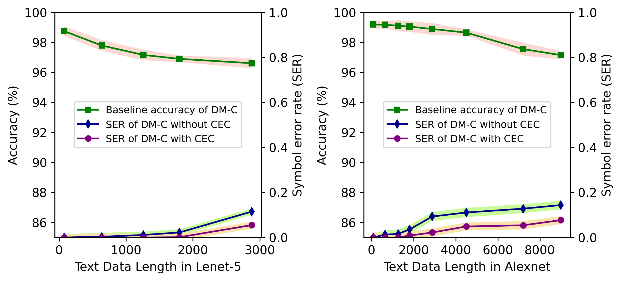
Figure 16: With the increasing number of text data, baseline accuracy is degrading, and the symbol error rate is showing an upward trend as we approach the capacity.

Text data has built-in redundancy since ASCII values are concentrated in a range that the network can efficiently learn [49, 21]. To get a true measure of capacity, we also communicated random data to the receiver using covert DeepMem (DM-C). We used different lengths of random data and report the symbol error rate of the channel as well as the accuracy degradation of baseline for both models shown in Figure 17.

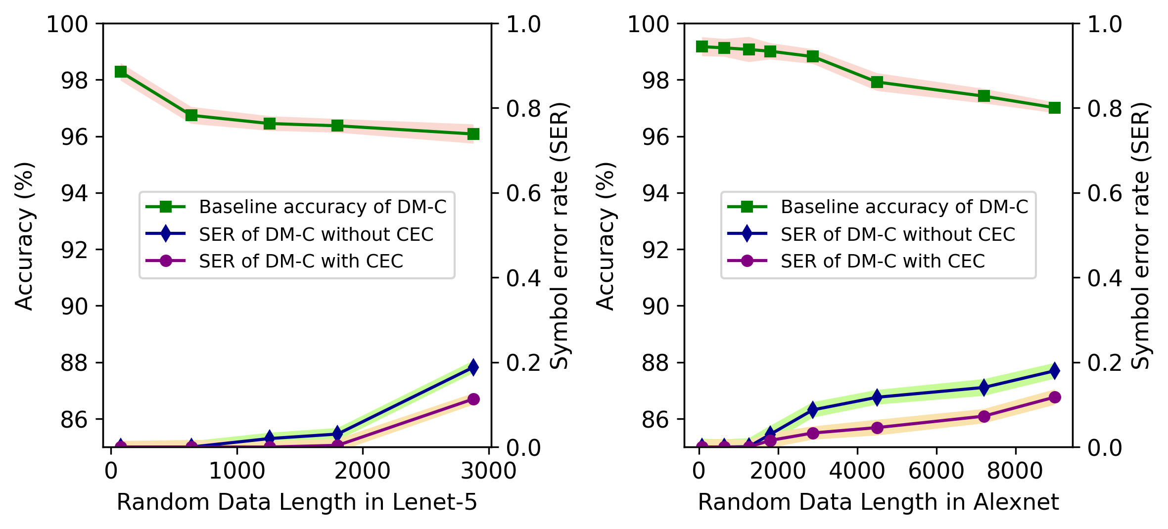
Figure 17: Random data: Baseline accuracy degrades, and symbol error rate increases as we approach capacity.

Figure 17 shows the results for sending random data, for message sizes similar to the text experiment. The behavior shows similar overall patterns. The accuracy drop for the same size was marginally higher (e.g., up to 2.66% drop from 98.74 to 96.08 on Lenet-5) as we increase the size of the random message, since the entropy of the random message is higher than that of text. As with text, CEC improves the symbol error rate.

Overall, DM-C requires significantly more examples for each address to learn the pattern reliably. As a result, overall the achievable capacity is lower than DM-DG. For example, on Lenet-5, for a similar drop in baseline accuracy, we were able to send messages of 20000 digits or higher reliably.

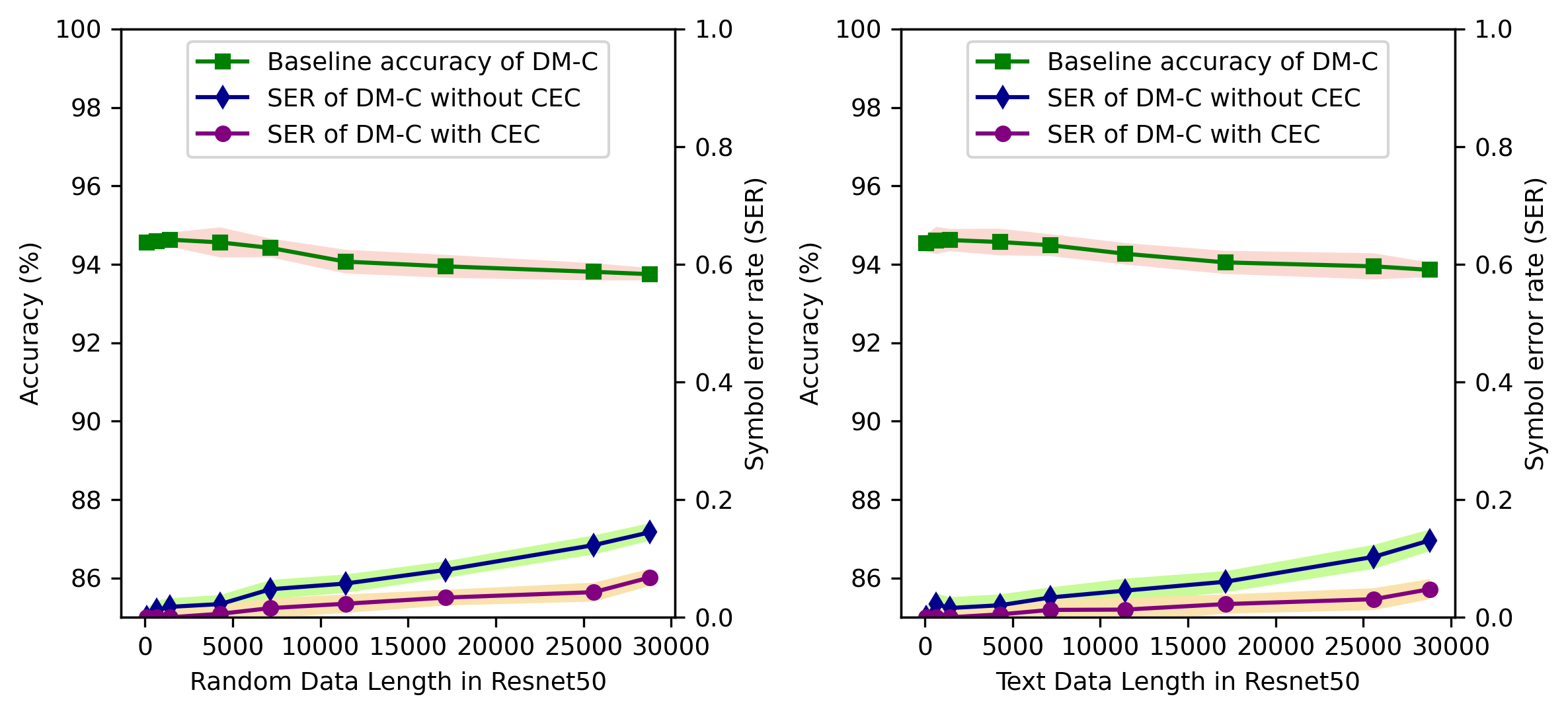
Figure 18: With the increasing number of random/text data, baseline accuracy is degrading, and the symbol error rate is showing an upward trend.

We also consider the capacity of DM-C on larger networks (Resnet50, with 23.5 million parameters) trained on the CIFAR10 dataset. Figure 18 shows the results of an experiment transferring both random and text data as we increase the message size. We sent up to 18000 digits of random data (3 bits each) with baseline accuracy degradation of 0.82 (from 94.57 to 93.75) shown in Figure 18.or the same length of text data, We observed the baseline accuracy degradation of 0.71 ( from 94.57 to 93.86) shown in Figure 18). For both types of data, we notice the same as other models that baseline accuracy degrades with the increasing size of the private data length and random data extraction accuracy degrades a little faster than text data. However, as Resnet50 has a large number of parameters, we can accommodate a high number of private data without substantially degrading the baseline accuracy.

6.2 Evaluating Covertness

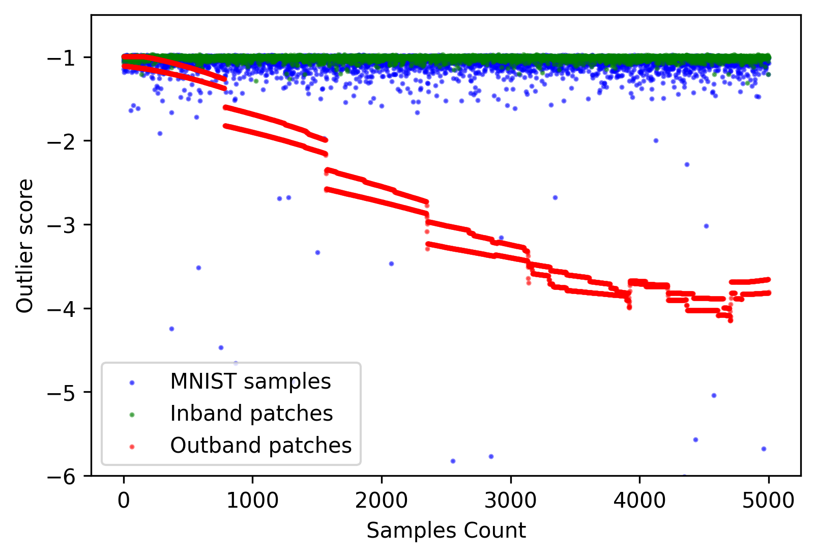
(a) Local Outlier Factor (LOF)

(b) Cosine Similarity

Figure 19: Outlier detection using (a) LOF and (b) Cosine Similarity. Baseline MNIST samples in blue dots, patched samples with Outside distribution in red dots and Inline distribution in green dots.

To evaluate DM-C for covertness, we examine both the inputs and the network to evaluate whether outliers can be detected.

Visualization in the input space. We use both LOF (shown in Figure 19(a)), and cosine similarity (in Figure 19(b)) metrics to visualize the distribution shift between the augmented data and the initial data distributions. Figure 19 implies that the approach for the address generation of covert DeepMem-BB is more amenable to hiding the poisoned data using small patch perturbation patterns (green dots in Figure 19) that are difficult to detect, whereas the outband images (red dots in Figure 19) are out of the original distribution and hence easily identifiable.

(a) DeepMem-Covert (DM-C)

(b) Baseline (DM-DG)

Figure 20: Visualization of the features learned by the Resnet50 model trained with CIFAR10 dataset. The color indicates the point’s class. Solid circle represents baseline classes and cross mark represents patched samples

Visualization in the features space. Figure 20 shows the features learned by ResNet50 trained on augmented CIFAR10 using covert DeepMem (DM-C)(Figure 20(a)) and baseline non-covert DeepMem (DM-DG)(Figure 20(b)). The points are sampled from the last dense layer of the model and then projected to 2D using t-SNE [76]. Figure 20(b) clearly demonstrates that the classes of the baseline samples (solid circle) and the classes of the patched samples (cross mark) are mostly distinguishable for the case of DM-DG because of the outside distribution patches compared to the initial data. However, for the case of DM-C shown in Figure 20(a), we notice that the clusters of the baseline data are overlapping with the patched samples.

7 Potential Mitigations

DeepMem leverages model overparametrization to create a communication channel that could enable communicating sensitive information through the model covertly and without harming the baseline task accuracy. The information is not directly injected into the model itself but rather hidden through an encoding strategy, which can be extracted by a colluding actor using predefined addresses. This mechanism can be effectively seen as a backdoor attack and the accuracy of this channel can potentially be degraded using the same defenses that are used against backdoor attacks, with minor to no modifications. Such defenses include Fine-tuning[44], Pruning[24], distillation[42, 77] and Ensemble techniques[35]. We investigate the most commonly used Fine tuning and Pruning defenses.We make the following realistic assumption: the receiver has access to a small fraction of trusted and unmodified data that it uses for fine tuning. In this section, we present the performance of the Pruning and Fine-tuning based defenses against both a covert and non-covert channel.

Pruning. In a model pruning defense, the smaller weights in the layers of the model are pruned (set to 0). The intuition behind pruning is that these smaller parameters do not contribute significantly to the operation of the network and can be removed. We perform pruning for 10 epochs and fine tune the model with 10% of training data from each class as common after pruning operations. Figure 21(a) illustrates how DM-C and DM-DG are affected by increasingly aggressive parameter pruning. The patch accuracy for both algorithms rapidly decreases although some signal remains even after pruning more than half the network. For DM-C, the baseline accuracy decreases rapidly with the pruning rate, but DM-DG’s baseline accuracy declines gradually and maintains $68\%$ even when we remove $99\%$ of Lenet-5 model’s parameters. It is interesting that the pruning impact is not the same for DM-C and DM-DG; for DM-C where the patches are sampled from the baseline distribution, the pruning affects simultaneously both the patch and the baseline accuracy. However, since DM-DG uses out-of-distribution patches, the pruning impacts patches earlier than the baseline accuracy.

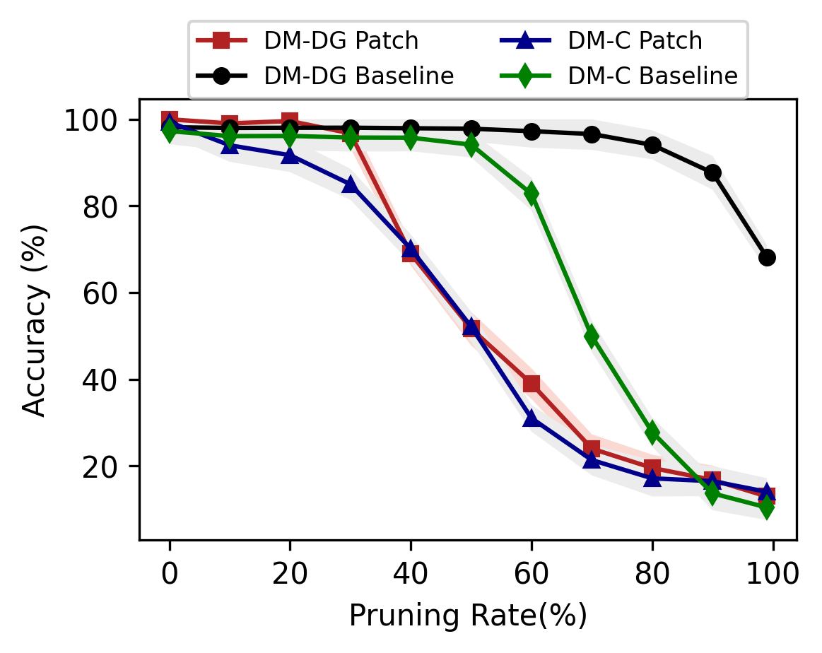
(a) Pruning

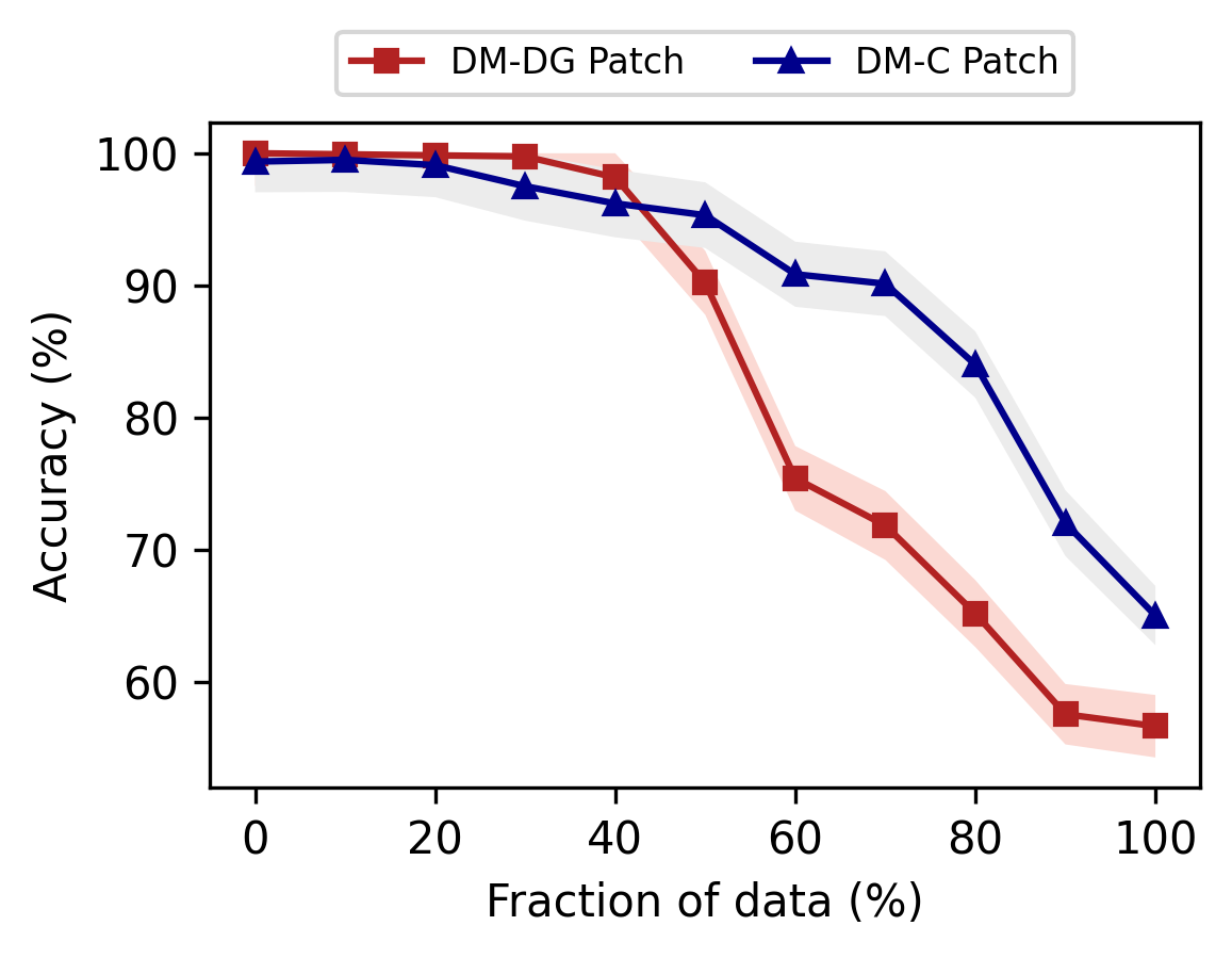
(b) Fine Tuning

Figure 21: Pruning and fine-tuning as a defense for DM-C and DM-DG on Lenet-5 with MNIST (data length 1260)

Fine-tuning. Another possible defense strategy is fine-tuning, where a fraction of clean new data is used to retrain the model so that the malicious behavior is overwritten. Intuitively, adding new training epochs would potentially push the model stored in the UPs since it is not reinforced. We retrain the final model for 10 epochs using an increasing fraction of the clean baseline training dataset in Figure 21(b).We notice that the patch accuracy of the DM-DG non-covert channel deteriorates more quickly than the DM-C covert channel. This can be explained by the use of baseline distribution in DM-C’s patched samples. The baseline accuracy was unchanged or improved slightly from the fine-tuning.

8 Related Work

Communicating private data. Among the recent works on communicating extra information through ML models are capacity abuse attack [72] and watermarking [66, 46]. Song et. al. [72] develop a malicious learning algorithm designed to train a model that leaks details about the training data. Rouhani et. al. [66] proposed DeepSigns that embeds a string watermark (maximum 512 bits) into the model by altering the probability distribution function (PDF) of the activation maps of a layer. Other watermark embedding techniques have been proposed in both white box [75, 57] and black box scenario [46, 40, 2] to protect the rights of ML model.

These works are the closest to our approach. While they embed information within the victim model in addition to the baseline task, there is no comprehensive evaluation of the extent/limit of the capacity that can be exploited. Besides, for the malicious data embedding works, especially [72], their approach did not consider covertness into account, which makes them easily detectable by simple analysis of the training set, as shown in Section 4.

Model hijacking. Several papers proposed to overload ML models with secondary tasks. Salem et al. [68] proposed ModelHijacking attack that hides a model covertly while training a victim model. Elsayed et. al. [26] proposed adversarial reprogramming in which instead of creating adversarial instances, they crafted inputs that would trick the network into performing new tasks. In the same direction, Mallya et. al [47] proposed Packnet that trains the model with multiple tasks.

Privacy Attacks. In the spirit of extracting information from a trained model, several works tried to exploit the ML model to leak sensitive information. Membership inference attacks that infer whether a specific data sample is part of the training dataset [70, 59, 82]. Property inference attacks infer specific properties of the training data distribution [84, 60, 16]. In model inversion attacks  [13, 30, 83] the adversary reconstructs the training data of the target model.

On a more advanced side, memorization concept has been investigated thoroughly in recent works. Specifically, several papers [11, 12, 14] demonstrated that large language models (LLM) are likely to unintentionally memorize a fraction of training data that contain duplicate sequences. Doubling the parameters in a model facilitates high memorization that leads to the extraction of a significantly larger fraction of the training data. As a possible countermeasure, deduplicating datasets have been suggested [41] to avoid memorization.

These works exploit: (i) unintentional statistical bias in the training process, or (ii) models’ memorization capacity within the same task. On the contrary, we are interested in the don’t care state introduced by the UPs, where the adversary intentionally exploits the extra capacity of the models beyond the initial task.

9 Concluding Remarks

In this paper, we propose a novel modeling of ML architectures, which we believe represents a general blueprint for several existing and potential future benign and malicious applications. We conceptualise ML models as communication channels with an effective capacity that increases with overparametrization. We show that using this approach, we can transfer arbitrary information without impacting the baseline task. We empirically characterize this capacity and propose write and read primitives allowing potential adversaries to communicate information in a black-box setting while being covert.

References

- [1] Martín Abadi. Tensorflow: learning functions at scale. In Proceedings of the 21st ACM SIGPLAN International Conference on Functional Programming, pages 1–1, 2016.
- [2] Yossi Adi, Carsten Baum, Moustapha Cisse, Benny Pinkas, and Joseph Keshet. Turning your weakness into a strength: Watermarking deep neural networks by backdooring. In 27th USENIX Security Symposium (USENIX Security 18), pages 1615–1631, 2018.
- [3] Mohammed Al-Qizwini, Iman Barjasteh, Hothaifa Al-Qassab, and Hayder Radha. Deep learning algorithm for autonomous driving using googlenet. In 2017 IEEE Intelligent Vehicles Symposium (IV), pages 89–96. IEEE, 2017.
- [4] Omar Alghushairy, Raed Alsini, Terence Soule, and Xiaogang Ma. A review of local outlier factor algorithms for outlier detection in big data streams. Big Data and Cognitive Computing, 5(1):1, 2020.
- [5] Md Zahangir Alom, Mahmudul Hasan, Chris Yakopcic, Tarek M Taha, and Vijayan K Asari. Recurrent residual convolutional neural network based on u-net (r2u-net) for medical image segmentation. arXiv preprint arXiv:1802.06955, 2018.
- [6] Filippo Arcadu, Fethallah Benmansour, Andreas Maunz, Jeff Willis, Zdenka Haskova, and Marco Prunotto. Deep learning algorithm predicts diabetic retinopathy progression in individual patients. NPJ digital medicine, 2(1):92, 2019.
- [7] Eugene Bagdasaryan, Andreas Veit, Yiqing Hua, Deborah Estrin, and Vitaly Shmatikov. How to backdoor federated learning. In International Conference on Artificial Intelligence and Statistics, pages 2938–2948. PMLR, 2020.
- [8] Battista Biggio, Blaine Nelson, and Pavel Laskov. Poisoning attacks against support vector machines. arXiv preprint arXiv:1206.6389, 2012.
- [9] Ekaba Bisong and Ekaba Bisong. An overview of google cloud platform services. Building Machine Learning and Deep Learning Models on Google Cloud Platform: A Comprehensive Guide for Beginners, pages 7–10, 2019.
- [10] Mariusz Bojarski, Davide Del Testa, Daniel Dworakowski, Bernhard Firner, Beat Flepp, Prasoon Goyal, Lawrence D Jackel, Mathew Monfort, Urs Muller, Jiakai Zhang, et al. End to end learning for self-driving cars. arXiv preprint arXiv:1604.07316, 2016.
- [11] Nicholas Carlini, Daphne Ippolito, Matthew Jagielski, Katherine Lee, Florian Tramer, and Chiyuan Zhang. Quantifying memorization across neural language models. arXiv preprint arXiv:2202.07646, 2022.
- [12] Nicholas Carlini, Matthew Jagielski, Chiyuan Zhang, Nicolas Papernot, Andreas Terzis, and Florian Tramer. The privacy onion effect: Memorization is relative. In S. Koyejo, S. Mohamed, A. Agarwal, D. Belgrave, K. Cho, and A. Oh, editors, Advances in Neural Information Processing Systems, volume 35, pages 13263–13276. Curran Associates, Inc., 2022.
- [13] Nicholas Carlini, Chang Liu, Úlfar Erlingsson, Jernej Kos, and Dawn Song. The secret sharer: Evaluating and testing unintended memorization in neural networks. In USENIX Security Symposium, volume 267, 2019.
- [14] Nicholas Carlini, Chang Liu, Úlfar Erlingsson, Jernej Kos, and Dawn Song. The secret sharer: Evaluating and testing unintended memorization in neural networks. In Proceedings of the 28th USENIX Conference on Security Symposium, SEC’19, page 267–284, USA, 2019. USENIX Association.
- [15] Nicholas Carlini and David Wagner. Towards evaluating the robustness of neural networks. In 2017 ieee symposium on security and privacy (sp), pages 39–57. IEEE, 2017.
- [16] Melissa Chase, Esha Ghosh, and Saeed Mahloujifar. Property inference from poisoning. arXiv preprint arXiv:2101.11073, 2021.
- [17] K. Chowdhary and G. Chowdhary. Natural language processing. Fundamentals of artificial intelligence, pages 603–649, 2020.
- [18] Antonia Creswell, Tom White, Vincent Dumoulin, Kai Arulkumaran, Biswa Sengupta, and Anil A Bharath. Generative adversarial networks: An overview. IEEE signal processing magazine, 35(1):53–65, 2018.
- [19] Bita Darvish Rouhani, Huili Chen, and Farinaz Koushanfar. Deepsigns: An end-to-end watermarking framework for ownership protection of deep neural networks. In Proceedings of the Twenty-Fourth International Conference on Architectural Support for Programming Languages and Operating Systems, pages 485–497, 2019.
- [20] Najim Dehak, Reda Dehak, James R Glass, Douglas A Reynolds, Patrick Kenny, et al. Cosine similarity scoring without score normalization techniques. In Odyssey, page 15, 2010.
- [21] Miguel Delgado, Maria J Martín-Bautista, Daniel Sánchez, and MA Vila. Mining text data: special features and patterns. In Pattern Detection and Discovery: ESF Exploratory Workshop London, UK, September 16–19, 2002 Proceedings, pages 140–153. Springer, 2002.
- [22] Li Deng. The mnist database of handwritten digit images for machine learning research. IEEE Signal Processing Magazine, 29(6):141–142, 2012.
- [23] Li Deng and Yang Liu. Deep learning in natural language processing. Springer, 2018.
- [24] Guneet S Dhillon, Kamyar Azizzadenesheli, Zachary C Lipton, Jeremy Bernstein, Jean Kossaifi, Aran Khanna, and Anima Anandkumar. Stochastic activation pruning for robust adversarial defense. arXiv preprint arXiv:1803.01442, 2018.
- [25] Ahmed El-Sawy, Hazem El-Bakry, and Mohamed Loey. Cnn for handwritten arabic digits recognition based on lenet-5. In International conference on advanced intelligent systems and informatics, pages 566–575. Springer, 2016.
- [26] Gamaleldin F Elsayed, Ian Goodfellow, and Jascha Sohl-Dickstein. Adversarial reprogramming of neural networks. arXiv preprint arXiv:1806.11146, 2018.
- [27] Nicole Fern, Shrikant Kulkarni, and Kwang-Ting Tim Cheng. Hardware trojans hidden in rtl don’t cares—automated insertion and prevention methodologies. In 2015 IEEE International Test Conference (ITC), pages 1–8, 2015.
- [28] Jonathan Frankle and Michael Carbin. The lottery ticket hypothesis: Finding sparse, trainable neural networks. arXiv preprint arXiv:1803.03635, 2018.
- [29] Jonathan Frankle, David J Schwab, and Ari S Morcos. The early phase of neural network training. arXiv preprint arXiv:2002.10365, 2020.
- [30] Matt Fredrikson, Somesh Jha, and Thomas Ristenpart. Model inversion attacks that exploit confidence information and basic countermeasures. In Proceedings of the 22nd ACM SIGSAC conference on computer and communications security, pages 1322–1333, 2015.
- [31] Clement Fung, Chris JM Yoon, and Ivan Beschastnikh. Mitigating sybils in federated learning poisoning. arXiv preprint arXiv:1808.04866, 2018.
- [32] Elena Garcia, Maria Antonia Jimenez, Pablo Gonzalez De Santos, and Manuel Armada. The evolution of robotics research. IEEE Robotics & Automation Magazine, 14(1):90–103, 2007.
- [33] Ian J Goodfellow, Jonathon Shlens, and Christian Szegedy. Explaining and harnessing adversarial examples. arXiv preprint arXiv:1412.6572, 2014.
- [34] Kaiming He, Xiangyu Zhang, Shaoqing Ren, and Jian Sun. Deep residual learning for image recognition. In Proceedings of the IEEE conference on computer vision and pattern recognition, pages 770–778, 2016.
- [35] Warren He, James Wei, Xinyun Chen, Nicholas Carlini, and Dawn Song. Adversarial example defense: Ensembles of weak defenses are not strong. In WOOT, pages 15–15, 2017.
- [36] Julia Hirschberg and Christopher D Manning. Advances in natural language processing. Science, 349(6245):261–266, 2015.
- [37] Briland Hitaj, Giuseppe Ateniese, and Fernando Perez-Cruz. Deep models under the gan: information leakage from collaborative deep learning. In Proceedings of the 2017 ACM SIGSAC Conference on Computer and Communications Security, pages 603–618, 2017.
- [38] Ling Huang, Anthony D Joseph, Blaine Nelson, Benjamin IP Rubinstein, and J Doug Tygar. Adversarial machine learning. In Proceedings of the 4th ACM workshop on Security and artificial intelligence, pages 43–58, 2011.
- [39] Alex Krizhevsky and Geoff Hinton. Convolutional deep belief networks on cifar-10. Unpublished manuscript, 40(7):1–9, 2010.
- [40] Erwan Le Merrer, Patrick Perez, and Gilles Trédan. Adversarial frontier stitching for remote neural network watermarking. Neural Computing and Applications, 32:9233–9244, 2020.
- [41] Katherine Lee, Daphne Ippolito, Andrew Nystrom, Chiyuan Zhang, Douglas Eck, Chris Callison-Burch, and Nicholas Carlini. Deduplicating training data makes language models better. arXiv preprint arXiv:2107.06499, 2021.
- [42] Yige Li, Xixiang Lyu, Nodens Koren, Lingjuan Lyu, Bo Li, and Xingjun Ma. Neural attention distillation: Erasing backdoor triggers from deep neural networks. arXiv preprint arXiv:2101.05930, 2021.
- [43] Ziwei Liu, Ping Luo, Xiaogang Wang, and Xiaoou Tang. Large-scale celebfaces attributes (celeba) dataset. Retrieved August, 15(2018):11, 2018.
- [44] Nils Lukas, Yuxuan Zhang, and Florian Kerschbaum. Deep neural network fingerprinting by conferrable adversarial examples. arXiv preprint arXiv:1912.00888, 2019.
- [45] Xinjian Luo, Yuncheng Wu, Xiaokui Xiao, and Beng Chin Ooi. Feature inference attack on model predictions in vertical federated learning. In 2021 IEEE 37th International Conference on Data Engineering (ICDE), pages 181–192. IEEE, 2021.
- [46] Peizhuo Lv, Pan Li, Shenchen Zhu, Shengzhi Zhang, Kai Chen, Ruigang Liang, Chang Yue, Fan Xiang, Yuling Cai, Hualong Ma, et al. Ssl-wm: A black-box watermarking approach for encoders pre-trained by self-supervised learning. arXiv preprint arXiv:2209.03563, 2022.
- [47] Arun Mallya and Svetlana Lazebnik. Packnet: Adding multiple tasks to a single network by iterative pruning. In Proceedings of the IEEE conference on Computer Vision and Pattern Recognition, pages 7765–7773, 2018.
- [48] Bishwas Mandal, Adaeze Okeukwu, and Yihong Theis. Masked face recognition using resnet-50. arXiv preprint arXiv:2104.08997, 2021.
- [49] Qiaozhu Mei and ChengXiang Zhai. Discovering evolutionary theme patterns from text: an exploration of temporal text mining. In Proceedings of the eleventh ACM SIGKDD international conference on Knowledge discovery in data mining, pages 198–207, 2005.
- [50] Luca Melis, Congzheng Song, Emiliano De Cristofaro, and Vitaly Shmatikov. Exploiting unintended feature leakage in collaborative learning. In 2019 IEEE Symposium on Security and Privacy (SP), pages 691–706. IEEE, 2019.
- [51] Riccardo Miotto, Fei Wang, Shuang Wang, Xiaoqian Jiang, and Joel T Dudley. Deep learning for healthcare: review, opportunities and challenges. Briefings in bioinformatics, 19(6):1236–1246, 2018.
- [52] Volodymyr Mnih, Koray Kavukcuoglu, David Silver, Alex Graves, Ioannis Antonoglou, Daan Wierstra, and Martin Riedmiller. Playing atari with deep reinforcement learning. arXiv preprint arXiv:1312.5602, 2013.
- [53] Christopher Z Mooney. Monte carlo simulation. Number 116. Sage, 1997.
- [54] Seyed-Mohsen Moosavi-Dezfooli, Alhussein Fawzi, and Pascal Frossard. Deepfool: a simple and accurate method to fool deep neural networks. In Proceedings of the IEEE conference on computer vision and pattern recognition, pages 2574–2582, 2016.
- [55] Robert H Morelos-Zaragoza. The art of error correcting coding. John Wiley & Sons, 2006.
- [56] Luis Muñoz-González, Battista Biggio, Ambra Demontis, Andrea Paudice, Vasin Wongrassamee, Emil C Lupu, and Fabio Roli. Towards poisoning of deep learning algorithms with back-gradient optimization. In Proceedings of the 10th ACM Workshop on Artificial Intelligence and Security, pages 27–38, 2017.
- [57] Yuki Nagai, Yusuke Uchida, Shigeyuki Sakazawa, and Shin’ichi Satoh. Digital watermarking for deep neural networks. International Journal of Multimedia Information Retrieval, 7:3–16, 2018.
- [58] Mohammad Naseri, Jamie Hayes, and Emiliano De Cristofaro. Toward robustness and privacy in federated learning: Experimenting with local and central differential privacy. arXiv preprint arXiv:2009.03561, 2020.
- [59] Milad Nasr, Reza Shokri, and Amir Houmansadr. Comprehensive privacy analysis of deep learning: Passive and active white-box inference attacks against centralized and federated learning. In 2019 IEEE symposium on security and privacy (SP), pages 739–753. IEEE, 2019.
- [60] Mathias PM Parisot, Balazs Pejo, and Dayana Spagnuelo. Property inference attacks on convolutional neural networks: Influence and implications of target model’s complexity. arXiv preprint arXiv:2104.13061, 2021.
- [61] Mansheej Paul, Brett W Larsen, Surya Ganguli, Jonathan Frankle, and Gintare Karolina Dziugaite. Lottery tickets on a data diet: Finding initializations with sparse trainable networks. arXiv preprint arXiv:2206.01278, 2022.
- [62] Harry A Pierson and Michael S Gashler. Deep learning in robotics: a review of recent research. Advanced Robotics, 31(16):821–835, 2017.
- [63] Aditya Ramesh, Prafulla Dhariwal, Alex Nichol, Casey Chu, and Mark Chen. Hierarchical text-conditional image generation with clip latents. arXiv preprint arXiv:2204.06125, 2022.
- [64] Aditya Ramesh, Mikhail Pavlov, Gabriel Goh, Scott Gray, Chelsea Voss, Alec Radford, Mark Chen, and Ilya Sutskever. Zero-shot text-to-image generation. In Marina Meila and Tong Zhang, editors, Proceedings of the 38th International Conference on Machine Learning, volume 139 of Proceedings of Machine Learning Research, pages 8821–8831. PMLR, 18–24 Jul 2021.
- [65] Joseph Redmon and Ali Farhadi. Yolo9000: Better, faster, stronger, 2016.
- [66] Bita Darvish Rouhani, Huili Chen, and Farinaz Koushanfar. Deepsigns: A generic watermarking framework for ip protection of deep learning models. arXiv preprint arXiv:1804.00750, 2018.
- [67] Jaakko Sahlsten, Joel Jaskari, Jyri Kivinen, Lauri Turunen, Esa Jaanio, Kustaa Hietala, and Kimmo Kaski. Deep learning fundus image analysis for diabetic retinopathy and macular edema grading. Scientific reports, 9(1):10750, 2019.
- [68] Ahmed Salem, Michael Backes, and Yang Zhang. Get a model! model hijacking attack against machine learning models. arXiv preprint arXiv:2111.04394, 2021.
- [69] C.E. Shannon. Communication in the presence of noise. Proceedings of the IRE, 37(1):10–21, 1949.
- [70] Reza Shokri, Marco Stronati, Congzheng Song, and Vitaly Shmatikov. Membership inference attacks against machine learning models. In 2017 IEEE Symposium on Security and Privacy (SP), pages 3–18. IEEE, 2017.
- [71] Karen Simonyan and Andrew Zisserman. Very deep convolutional networks for large-scale image recognition, 2014.
- [72] Congzheng Song, Thomas Ristenpart, and Vitaly Shmatikov. Machine learning models that remember too much. In Proceedings of the 2017 ACM SIGSAC Conference on computer and communications security, pages 587–601, 2017.
- [73] Ziteng Sun, Peter Kairouz, Ananda Theertha Suresh, and H Brendan McMahan. Can you really backdoor federated learning? arXiv preprint arXiv:1911.07963, 2019.
- [74] Marvin Teichmann, Michael Weber, Marius Zoellner, Roberto Cipolla, and Raquel Urtasun. Multinet: Real-time joint semantic reasoning for autonomous driving. In 2018 IEEE intelligent vehicles symposium (IV), pages 1013–1020. IEEE, 2018.
- [75] Yusuke Uchida, Yuki Nagai, Shigeyuki Sakazawa, and Shin’ichi Satoh. Embedding watermarks into deep neural networks. In Proceedings of the 2017 ACM on international conference on multimedia retrieval, pages 269–277, 2017.
- [76] Laurens Van der Maaten and Geoffrey Hinton. Visualizing data using t-sne. Journal of machine learning research, 9(11), 2008.
- [77] Bolun Wang, Yuanshun Yao, Shawn Shan, Huiying Li, Bimal Viswanath, Haitao Zheng, and Ben Y Zhao. Neural cleanse: Identifying and mitigating backdoor attacks in neural networks. In 2019 IEEE Symposium on Security and Privacy (SP), pages 707–723. IEEE, 2019.
- [78] Xi Wang, Nickolai Zeldovich, M Frans Kaashoek, and Armando Solar-Lezama. Towards optimization-safe systems: Analyzing the impact of undefined behavior. In Proceedings of the Twenty-Fourth ACM Symposium on Operating Systems Principles, pages 260–275, 2013.
- [79] Stephen B Wicker and Vijay K Bhargava. Reed-Solomon codes and their applications. John Wiley & Sons, 1999.
- [80] Wired. A New Chip Cluster Will Make Massive AI Models Possible. https://www.wired.com/story/cerebras-chip-cluster-neural-networks-ai/. Accessed: 2023-11-23.
- [81] Zheng-Wu Yuan and Jun Zhang. Feature extraction and image retrieval based on alexnet. In Eighth International Conference on Digital Image Processing (ICDIP 2016), volume 10033, pages 65–69. SPIE, 2016.
- [82] Jingwen Zhang, Jiale Zhang, Junjun Chen, and Shui Yu. Gan enhanced membership inference: A passive local attack in federated learning. In ICC 2020-2020 IEEE International Conference on Communications (ICC), pages 1–6. IEEE, 2020.
- [83] Yuheng Zhang, Ruoxi Jia, Hengzhi Pei, Wenxiao Wang, Bo Li, and Dawn Song. The secret revealer: Generative model-inversion attacks against deep neural networks. In Proceedings of the IEEE/CVF conference on computer vision and pattern recognition, pages 253–261, 2020.
- [84] Junhao Zhou, Yufei Chen, Chao Shen, and Yang Zhang. Property inference attacks against gans. arXiv preprint arXiv:2111.07608, 2021.