Towards Accelerating Benders Decomposition via
Reinforcement Learning Surrogate Models

Abstract

Stochastic optimization (SO) attempts to offer optimal decisions in the presence of uncertainty. Often, the classical formulation of these problems becomes intractable due to (a) the number of scenarios required to capture the uncertainty and (b) the discrete nature of real-world planning problems. To overcome these tractability issues, practitioners turn to decomposition methods that divide the problem into smaller, more tractable sub-problems. The focal decomposition method of this paper is Benders decomposition (BD), which decomposes stochastic optimization problems on the basis of scenario independence. In this paper we propose a method of accelerating BD with the aid of a surrogate model in place of an $\mathcal{NP}$-hard integer master problem. Through the acceleration method we observe $30\%$ faster average convergence when compared to other accelerated BD implementations. We introduce a reinforcement learning agent as a surrogate and demonstrate how it can be used to solve a stochastic inventory management problem.

1 Introduction

Optimization is frequently subject to conditions of uncertainty. If this uncertainty is not sufficiently accounted for by a solution, even minor perturbations in the environment can devalue results and lead to catastrophic outcomes. While uncertainty can often be simulated or even parameterized, solving over that uncertainty offers incredible complexity. To make optimal decisions that consider both the uncertainty and constraints of a system, the field of SO is often applied. SO considers a distribution of possible scenarios rather than a deterministic event, and seeks an optimal outcome across the range of possibilities.

A common challenge for stochastic optimization is tractability. Generating an optimal decision that considers its outcome across a large number of scenarios can be extremely costly. To combat these computational issues, a common approach is to decompose the problem into simpler and independent sub-problems that can be combined to retrieve a global certificate of optimality. In this paper, we offer an adaptation of the common decomposition method of Benders decomposition (BD).

Despite wide usage since its introduction, BD suffers from two well-known practical limitations. First, in discrete space, BD relies on an $\mathcal{NP}$-hard mixed-integer master problem (MIMP). This MIMP is responsible for making global decisions that are homogeneous across scenarios. Second, with each iteration a set of scenario-specific sub-problems (SP) generate gradient approximations that are passed to the MIMP as constraints (or cuts). The result is a MIMP with complexity that scales linearly with the number of required iterations as constraints are added.

Given these deficiencies, accelerating BD has become a compelling research problem. In production routing applications, (Adulyasak et al., 2015) implement lower-bound lifting inequalities to tighten initial lower bounds, and exploit scenario grouping to reduce added complexity at each iteration. (Baena et al., 2020) attempt to localize the loss approximation of BD by restricting each iteration to a subspace centered around strong past solutions. (Crainic et al., 2016) aid initial iterations by including an informative subset of scenarios within the MIMP. (Lee et al., 2021) offer a machine learning approach to predicting constraint importance; retaining only important cuts and limiting MIMP complexity. Each of these proposals has shown computational benefits, but remain solely dependent on the expensive MIMP to generate successive solutions. In contrast, (Poojari and Beasley, 2009) replace the MIMP with a genetic algorithm to produce faster feasible solutions. Although the heuristic produces fast master problem (MP) solutions, it is still reliant on SP approximations to undertstand scenario loss, and offers feasible as opposed to certifiably optimal solutions.

Our proposal introduces a surrogate model to quickly generate solutions to the discrete MP rather than relying on the MIMP. This surrogate generates fast solutions to unseen problems after learning the loss of decisions in similar stochastic environments. At varying rates, the MIMP is still run to retrieve the certificate of optimality offered by BD. In total, our contributions are:

• A generalized method of accelerating BD that retrieves optimal solutions to stochastic optimization problems while drastically reducing run times.

• A solution selection method that uses cuts from BD sub-problems to inform selection of future surrogate MP solutions; offering a further unification of the surrogate MP within the BD framework.

• A worked inventory management problem with detailed implementation of the acceleration method. We offer an explicit Benders formulation, and leverage an RL model as our surrogate MP.

• Experiments showing a $30\%$ reduction in run-time vs alternative acceleration methods.

2 Background

A widely used form of stochastic optimization is Sample Average Approximation (SAA). SAA aims to approximate loss over the distribution of possible scenarios using simulation. In SAA, $R$ scenarios are simulated, with each simulation yielding its own deterministic sub-problem with a loss function $f(x,w,D_{r})$, where $x$ is a set of global decisions (universal across all scenarios), $w$ is a cost vector, and $D_{r}$ is a set of scenario-specific parameters. The total loss of the problem is then computed as an average of the loss across all scenarios,

$$\ell(x)=\frac{1}{R}\sum_{\forall r\in R}f(x,w,D_{r})$$ (1)

Despite success in a number of optimal planning domains, the struggles of scaling SO problems are well documented. For example, (Gendreau et al., 1996) note that when solving stochastic vehicle routing problems, practitioners commonly resort to comparing heuristics as exact methods become intractable. To combat scalability issues, decomposition methods are commonly employed to solve large-scale SO problems. Here we introduce the principles of Benders decomposition. Consider an SAA problem of the form:

$$\min_{x,y}c^{T}x+\frac{1}{R}\sum_{\forall r\in R}w^{T}y_{r}$$ (2)

subject to

$$Ax=b$$ (3)

$$Bx+D_{r}y_{r}=g,\qquad\forall r\in R$$ (4)

$$x\in\mathbb{Z},y_{r}\in\mathbb{Z}^{+},\qquad\forall r\in R$$ (5)

where $x$ is again our set of global decisions, $A$, $b$, and $B$ are parameters that define constraints on $x$, $c$ is the cost of global decisions, $D_{r}$ and $g$ are scenario-specific parameters, $y_{r}$ is a set of decisions made independently within each scenario, and $w$ is a cost applied to each scenario-specific decision. In this formulation, $w^{T}y_{r}$ is equivalent to (1). The first step of BD is to separate the global decision variables $x$ and scenario-specific decision variables $y_{r}$. This leaves us with a master problem

$$\{\min_{x,\theta}c^{T}x+\frac{1}{R}\sum_{\forall r\in R}\theta_{r}:Ax=b,x\in\mathbb{Z}^{+}\}$$ (6)

and a collection of $R$ sub-problems, where for each $r\in R$ we have

$$\{\min_{y_{r}}w^{T}y_{r}:D_{r}y_{r}=g-Bx^{*},y_{r}\in\mathbb{R}^{+}\}$$ (7)

The sub-problems accept a fixed $x^{*}$ based on the solution to (6), and are solved to obtain optimal sub-problem decisions $y_{r}$. Note that BD introduces a set of auxiliary variables $\theta_{r},\forall r\in R$ to the master problem (6). This auxiliary variable, frequently called the recourse variable, is responsible for tracking an approximation of the sub-problem loss that has been moved to (7). Let us assume the sub-problem is always feasible. This is not a necessary assumption, but simplifies the following description of BD.

Note that integrality on $y_{r}$ has been relaxed in the sub-problem. This relaxation is necessary for Benders decomposition, and only possible when a) the sub-problem variables were not discrete to begin with or b) the decomposition results in a totally-unimodular sub-problem structure. Taking the dual of the sub-problem, we get:

$$\{\max_{q_{r}}q_{r}^{T}(g-Bx^{*}):q_{r}^{T}D_{r}\leq w\}$$ (8)

The dual sub-problem has three essential properties. First, through strong duality the optimal value of (8) is equivalent to the optimal value of (7) at $x^{*}$. Second, the objective function (8) is linear with respect to the master problem decisions $x$. And lastly, with the optimal dual values of $q^{*}_{r}$ we can establish

$$\{min_{y_{r}}w^{T}y_{r}:D_{r}y_{r}=g-Bx\}\geq\\ q_{r}^{*T}(g-Bx),\forall x\in\mathbb{R},\forall w\in\mathbb{R}$$ (9)

via weak duality. With these traits established, we see that the optimal dual SP objective $q_{r}^{*T}(g-Bx)$ can be included as a valid constraint on $\theta_{r}$ in the MIMP. These constraints serve as a sub-gradient approximations of the SP loss. For each SP solution, we can update the MIMP with the valid constraint of $\theta_{r}\geq q_{r}^{*T}(g-Bx)$ and re-solve for a new $x$. This process is repeated until the SP’s do not offer any strengthening constraints on $\theta_{r}$, indicating convergence and full approximation of SP loss. Figure 1 offers a visual representation of this process.

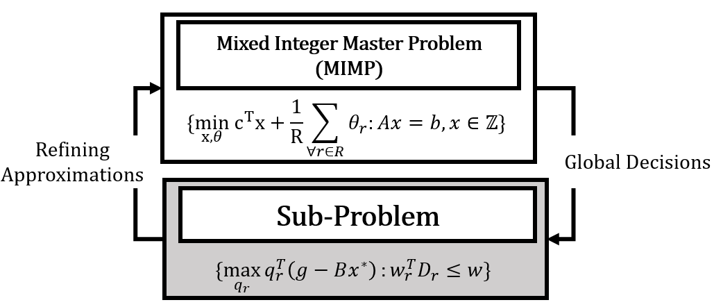
Figure 1: Iterative procedure of Benders decomposition, alternating between a MIMP (6) and SP (8).

2.1 Reinforcement Learning

Reinforcement Learning (RL) offers a powerful approach to solving combinatorial problems. (Delarue et al., 2020) gives one such example of RL applied to combinatorial problems, solving notoriously challenging capacitated vehicle routing problems using value-based methods. As shown in (Delarue et al., 2020), the benefit of RL-based methods is that after learning a near-optimal policy, they can generate actions in discrete space very quickly, albeit without a guarantee of optimality.

RL is typically based on the Markov Decision Process (MDP) framework as described by Sutton and Barto (Sutton and Barto, 2018). This can be defined by a tuple $\langle\mathcal{S},\mathcal{A},\mathcal{T},\mathcal{R}\rangle$ where $\mathcal{S}$ is the set of states, $\mathcal{A}$ is the set of actions, $\mathcal{T}$ is a set of transition probabilities from state $s$ to the next state $s^{\prime}$, and $\mathcal{R}$ is the reward function. In temporal environments, we can adopt the notation of $s_{t}\in\mathcal{S}$, $a_{t}\in\mathcal{A}$ for the state and action of a given time step $t$.

In RL, an agent attempts to learn the optimal action in a given state. Performance is measured by the collective rewards over future states and actions. The behaviors of the agent are updated based on prior experience, and can collectively be defined by a policy, $\boldsymbol{\pi}(s,a)$. RL algorithms can be broadly partitioned into two classes: value-based and policy based. In a value-based implementations, the policy $\boldsymbol{\pi}(s,a)$ is selected using value-function approximation methods, where

$$Q^{\boldsymbol{\pi}}(s_{t},a_{t})=\sum_{\forall j\in T}\mathbb{E}_{s_{t+1},a_{t+1},...}[\gamma_{t}\mathcal{R}(s_{t+j},a_{t+j})]$$ (10)

is the expected reward of an action, $\gamma_{t}$ is a discount rate placed on future reward, and an optimal policy is deterministically selected based on $argmax_{\boldsymbol{\pi}}Q^{\boldsymbol{\pi}}$.

Rather than estimating the value-function $Q$ and generating policies based on actions that maximize that approximation, policy-based reinforcement learning aims to optimize a functional representation of the policy $\boldsymbol{\pi}(s,a)$. We define the functional representation of a policy as $\boldsymbol{\pi}_{\boldsymbol{\beta}}(s,a)$, where $\boldsymbol{\beta}$ is a set of learned parameters. Importantly, in policy-based learning the agent optimizes the parameters $\boldsymbol{\beta}$ to generate a stochastic policy. This stochastic policy respects the fact that the cumulative reward for an action may not be deterministic, and consequentially a single best action may not exist.

Work from (Sutton et al., 1999) introduces an optimization procedure for policy-based RL that updates the parameter set $\boldsymbol{\beta}$ via an estimate of the policy gradient. A powerful variation of policy-based optimization was introduced by (Schulman et al., 2017) to avoid detrimentally large policy updates. In their version of policy-based optimization, the policy changes are regulated by limiting the reward of policy variation. Their method, titled Proximal Policy Optimization (PPO), updates the objective function to clip the reward of policy updates where the ratio $|\frac{\boldsymbol{\pi}_{\boldsymbol{\beta}}^{new}(a_{t}|s_{t})}{\boldsymbol{\pi}_{\boldsymbol{\beta}}^{old}(a_{t}|s_{t})}|$ extends beyond some $\epsilon$.

Policy-based RL is a more applicable form of RL for our proposal, as it enables a set of diverse actions to be generated in a given state. Given a requirement for non-deterministic actions, our working example implements a PPO RL algorithm with a multi-layer neural network serving as our agent. The parameter set of this network, $\boldsymbol{\beta}$, defines our policy $\boldsymbol{\pi}_{\boldsymbol{\beta}}$.

3 Accelerating Benders Decomposition

With background on BD and RL provided, we introduce our proposed method of accelerating Benders decomposition. First, we will offer specifics on how a surrogate model is used in place of the MIMP. Then, we will introduce three possible mechanisms for selecting actions from the surrogate model. Lastly, we will offer a more thorough coverage of the theoretical benefits that the surrogate model provides, and known deficiencies of BD that it addresses.

3.1 Surrogate-MP

Recall the iterative procedure outlined in figure 1. The SP’s can be solved efficiently using any standard LP solver, but each iteration calls back to a complex MIMP. Not only is the MIMP $\mathcal{NP}$-hard, but its complexity scales linearly with the number of iterations as a new constraint is added from the SP. Given these mechanics, there is a strong desire to a) increase the speed of each master problem iteration and b) decrease the total number of calls to the MIMP required. We achieve both results by periodically introducing a faster surrogate model in place of the MIMP (figure 2). This surrogate model can be any model that has learned to map the stochastic input space to the discrete decision space with intentions of minimizing the problem loss. Later in the paper, we introduce an RL agent as our surrogate model to generate master problem solutions. We call this framework Surrogate-MP.

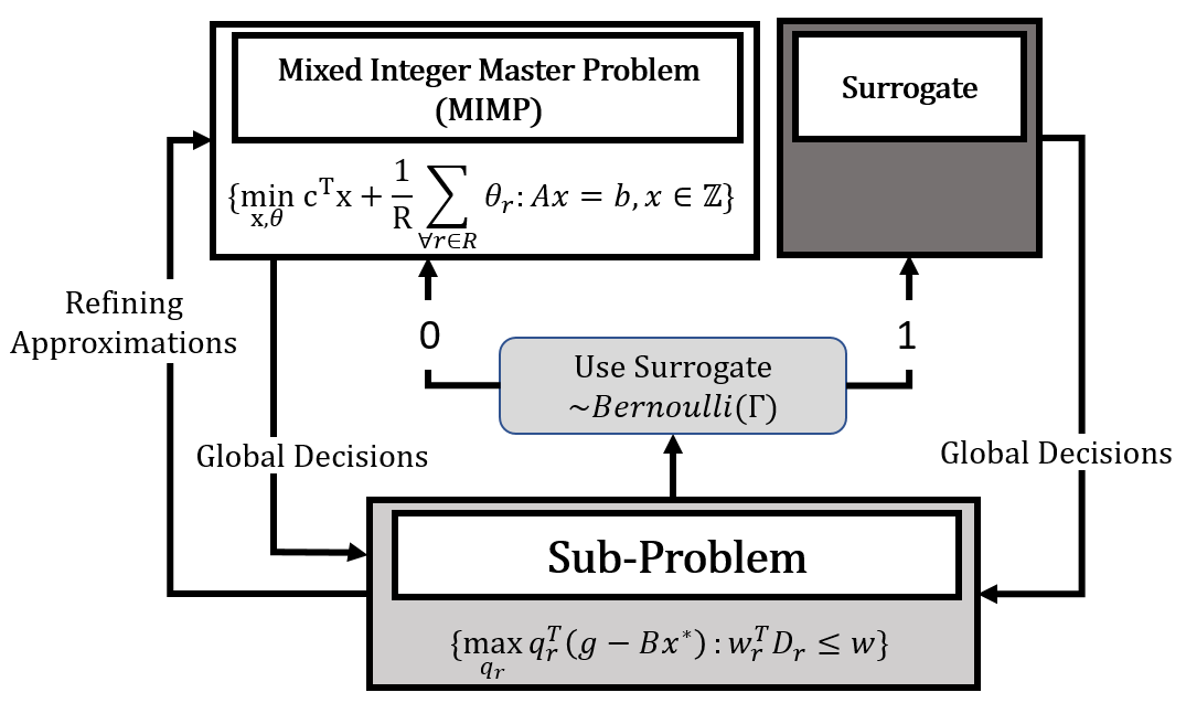
Figure 2: Iterative procedure of Surrogate-MP.

Note in this modified schema that with each iteration, the decision to use the surrogate in place of the MIMP is drawn from a Bernoulli distribution with a control parameter $\Gamma$. If a value of 1 is returned from the Bernoulli distribution, the surrogate is used to generate global decisions. Otherwise, the standard MIMP is run and the optimality gap can be confirmed. Regardless of whether the MIMP or surrogate are used, global decisions are passed to the sub-problem and loss approximating cuts are added.

3.2 Controlling Surrogate Usage

The surrogate model usage can be controlled in a variety of ways, and we offer three forms of control. These variants are aimed at answering (1) How frequently should we use the surrogate? (2) How can we be sure the surrogate solutions are useful for convergence? (3) If surrogate actions are non-deterministic, how can we decide which action are best to use? The three methods we implement are a greedy selection, weighted selection, and informed selection. Each of these methods assume the surrogate has generated a non-deterministic batch of actions for the given environment.

Greedy Selection

The greedy selection process first evaluates every surrogate solution in a batch against the expectation of demand over the horizon to estimate solution performance. At each iteration, the decision to use the surrogate is made with some probability. If the surrogate is used, we select the top performing solution from the batch and use it as our MP solution. The solution is then removed from the batch and the process is continued.

Weighted Selection

Rather than deterministically selecting actions based on their performance against an expectation, we can perform weighted random sampling. We again use the calculated loss of action $i$ evaluated against expected demand, which we call $\ell_{i}$. However, instead of selecting $argmin_{i}(\ell_{i})$ as in the greedy method, we create a probability vector, where $p(i)=\frac{\frac{1}{\ell_{i}}}{\sum_{\forall i\in I}\frac{1}{\ell_{i}}}$. Using this probability vector, we perform weighted sampling from the batch of actions each time the surrogate is called.

Informed

The final proposal is observed to be strongest in our experiments, and incorporates feedback from the BD sub-problems. With informed selection, surrogate solutions are selected using the constraint set currently placed on $\theta_{r}$. The benefit of utilizing the constraint matrix to select surrogate solutions is that these constraints inherently motivate exploration to either a) minimal or b) poorly approximated regions of the convex loss. Given final convergence is defined by a binding subset of these constraints, it is necessary to explore these minimal or poorly approximated regions.

To describe the method, we introduce a constraint matrix $A_{r}\in\mathbb{R}^{I\times N}$ which contains the sub-gradient approximations imposed on $\theta_{r}$, and a row vector of constant values $c_{r}\in\mathbb{R}^{I}$ that is added to each sub-gradient approximation. $I$ refers to the iteration number of BD, $N$ refers to the number of MP decision variables, and $r$ refers to the scenario.

Note each iteration generates a new set of sub-gradient approximations that are added to the matrix. As mentioned, these are the same sub-gradients that are applied to $\theta_{r}$ in the master problem, and are generated using our dual sub-problem. On a given iteration, we have a batch of $M$ solutions that have been generated by the surrogate. Decisions for this batch are represented by matrix $D\in\mathbb{Z}^{N\times M}$. We begin by computing the loss approximations of each gradient, for each of the $M$ solutions. This is given as $TCA_{r}\in\mathbb{R}^{I\times M}$.

$$TCA_{r}=A_{r}\cdot D+(\mathbb{c_{r}}\cdot 1^{1\times I})^{T}$$ (11)

The $TCA_{r}$ matrix contains approximations of the sub-problem loss for each of the $M$ solutions, generated by each of the $I$ constraints currently placed on $\theta_{r}$. We can now take the maximum value for each column $M$ as the approximated cost of solution $m$. In LP terms, this maximum value relates to the binding constraint on $\theta_{r}$ in the MIMP, and is thus our true approximation of SP cost at that point. We represent this approximation ($\ell_{mr}$) as:

$$\ell_{m,r}=\max_{\forall i\in I}(TCA_{r})_{im}$$ (12)

Now we fully approximate the expected loss for each of the $M$ solutions by taking an average across all $R$ scenarios, and adding the fixed loss of that decision (denoted $f_{m}$).

$$\ell_{m}=\frac{1}{R}\sum_{\forall r\in R}\ell_{m,r}+f_{m}$$ (13)

the surrogate solution that minimizes the problem

$$argmin_{m}\ell_{m}$$ (14)

is then taken as our MP solution, and passed to the sub-problem for constraint generation.

3.3 Benefits of Surrogate-MP

The benefits of using a surrogate model with learned actions in place of the MIMP is based on two central principles.

1. The time required to generate solutions from a pre-trained surrogate model is negligible compared to the time required to solve a large scale MIP.

2. The surrogate model has learned its actions from past exposure to the stochastic environment. As a result, sub-problem loss is expressed in surrogate model solutions regardless of how well $\theta_{r}$ approximates SP loss. This means that even early iterations of the surrogate model will be highly reflective of sub-problem loss.

The first benefit is fairly self-explanatory; we desire faster MP solutions, and the surrogate provides them. The second benefit is more nuanced and worth expanding. We recall the general form MIMP (6), where $\theta_{r}$ offers an approximation of sub-problem loss that is refined through linear constraints generated by (8). It is well observed that this approximation can converge quickly if global decisions are localized to the optimal region, but it can also be very slow if global decisions are far from the optimal region or the cuts poorly approximate the loss (Crainic et al., 2016; Baena et al., 2020). At initialization, $\theta_{r}$ has not received any feedback from the SP, and is instead bound by some heuristic or known lower bound (commonly $\theta_{r}\geq 0$ for non-negative loss). Given the lack of information initially imparted on $\theta_{r}$, the MP generates global solutions that lack consideration of SP loss and can be very distant from the optimal region. Similar to a gradient based algorithm with a miss-specified learning rate, this can lead BD to oscillate around the minimal region or converge slowly, wasting compute and adding complexity with minimal benefit to the final solution (Baena et al., 2020).

The surrogate mitigates this major issue by generating global decisions that reflect an understanding of their associated SP loss without requiring strong loss approximations on $\theta_{r}$. As a result, initial global decisions generated by the surrogate are localized to the minimal region and cuts can quickly approximate the minimum of the convex loss. These two fundamental benefits are the basis for a $30\%$ reduction in run-times, observed in experiments with the working example that follows.

4 Working Example

Let us introduce an inventory management problem (IMP) as a working example. In the proposed IMP, we assume the required solutions must a) choose a delivery schedule from a finite set, b) decide an order-up-to amount (order = order-up-to - current inventory) for each order day, and c) place costly emergency orders if demand cannot be met with current inventory. For simplicity we consider a single-item, single-location ordering problem where there is a requirement to satisfy all demand using either planned schedules, or more costly just-in-time emergency orders. The demand estimate is generated using a forecast model with an error term from an unknown probability distribution.

Adaptations of the general form IMP are applied in industries ranging from financial services, to brick-and-mortar retail. In e-commerce, vendors make decisions to either assume the holding costs associated with stocking inventory near demand locations, or use more costly fulfillment options to meet consumer needs (Arslan et al., 2021). In commercial banking, cash must be held at physical locations and made available to customers when needed, with a compounding cost of capital being applied to any unused cash (Ghodrati et al., 2013). Or in commodities trading, physical assets may need to be purchased and held until a desired strike price is realized in the future (Goel and Gutierrez, 2011).

4.1 SO Formulation and Decomposition

To model the IMP as a SO mixed-integer problem we introduce the following notation: let $T$ be set of days $t$, $R$ be set of scenarios $r$, and $S$ define a finite set of schedules $s$. Holding cost of an item (per unit-of-measure, per day) is $h$, the cost of emergency services (per unit) is $e$, the penalty applied to over-stocking (per unit over-stocked) is $q$, and $f_{s}$ is the fixed cost of a schedule. Capacity is defined by $m$ and starting inventory by $y$. The parameter $w_{st}$ indicates whether schedule $s$ orders on day $t$. Demand on day $t$ under scenario $r$ is $n_{tr}$.

The decision space is defined by seven sets of variables. The decision to use schedule $s$ is made using variable $u_{s}\in\{0,1\}$. The order-up-to amount is decided by $a_{t}\in\mathbb{Z}^{+}$, and $k_{tr}\in\mathbb{Z}$ is the required order quantity to meet the order-up-to amount. Inventory on hand is monitored by $d_{tr}\in\mathbb{Z}^{+}$, the units of holding space required to stock the inventory is $p_{tr}\in\mathbb{Z}^{+}$, the required emergency order quantity is $o_{tr}\in\mathbb{Z}^{+}$, and $v_{tr}\in\mathbb{Z}^{+}$ is the number of units that inventory is over-filled by (all defined $\forall t\in T,\forall r\in R$). The formulation of our IMP is

$$min\sum_{\forall s\in S}(u_{s}f_{s})+\frac{1}{R}\sum_{\forall r\in R}\sum_{\forall t\in T}(p_{tr}h+o_{tr}e+v_{tr}q)$$ (15)

subject to:

$$d_{tr}=y-n_{tr}+k_{tr}-v_{tr}+o_{tr},t=0,\forall r\in R$$ (16)

$$d_{tr}=d_{t-1,r}+k_{tr}-n_{tr}+o_{tr}-v_{tr},\forall t\in\{1,...,T\},\forall r\in R$$ (17)

$$p_{tr}\geq y+k_{tr}-v_{tr},t=0,\forall r\in R$$ (18)

$$p_{tr}\geq a_{t},\forall t\in\{1,...,T\},\forall r\in R$$ (19)

$$p_{tr}\geq p_{t-1,r}-a_{t},\forall t\in\{1,...,T\},\forall r\in R$$ (20)

$$y+k_{tr}-v_{tr}\leq m,t=0,\forall r\in R$$ (21)

$$d_{t-1,r}+k_{tr}-v_{tr}\leq m,\forall t\in\{1,...,T\},\forall r\in R$$ (22)

$$k_{tr}=a_{t}-y\sum_{\forall s\in S}u_{s}w_{st}$$ (23)

$$k_{tr}\geq a_{t}-d_{t-1,r},\forall t\in\{1,...,T\},\forall r\in R$$ (24)

$$k_{tr}\leq a_{t}-d_{t-1,r}+(1-\sum_{\forall s\in S}u_{s}w_{st})m,\forall t\in\{1,...,T\},\forall r\in R$$ (25)

$$k_{tr}\leq a_{t},\forall t\in T,\forall r\in R$$ (26)

$$k_{tr}\geq-\sum_{\forall s\in S}u_{s}w_{st}\times m,\forall t\in T,\forall r\in R$$ (27)

$$v_{tr}\leq a_{t},\forall t\in T,\forall r\in R$$ (28)

$$a_{t}\leq\sum_{\forall s\in S}u_{s}w_{st}\times m,\forall t\in T$$ (29)

$$\sum_{\forall s\in S}u_{s}=1$$ (30)

The objective (15) minimizes the sum of planned schedule costs and the average of holding costs, emergency order costs, and over-fill costs across the $R$ scenarios. Flow constraints (16) and (17) balance inflow and outflow of inventory through demand and deliveries. The holding cost is enforced by constraints (18), (19), and (20). Constraints (21) and (22) mandate that inventory cannot be filled beyond its capacity. Lastly, constraints (23), (24), (25), (26), (27), (28), and (29) ensure an order exactly fills the inventory to the optimal order-up-to-amount, and that orders are only placed on scheduled days. (30) guarantees exactly one schedule is selected.

For BD, we note that $\mathbb{a}$ and $\mathbb{u}$ are schedule and order-up-to decisions that must be made the same across all scenarios. As a result, $\mathbb{a}$, $\mathbb{u}$, (29), and (30) are contained in the MIMP while the remaining decision variables and constraints are delegated to the scenario specific sub-problems. For brevity, we omit the primal sub-problem formulation and directly introduce the cut-generating dual sub-problem formulation. We define the dual variables in line with their related constraints: $\boldsymbol{\alpha}\in\mathbb{R}$ [(16), (17)], $\boldsymbol{\gamma}\in\mathbb{R}^{+}$ [(18), (19)], $\boldsymbol{\omega}\in\mathbb{R}^{+}$ (20), $\boldsymbol{\phi}\in\mathbb{R}^{+}$ [(21),(22)], $\boldsymbol{\xi^{0}}\in\mathbb{R}$ (23), $\boldsymbol{\xi^{lb}}\in\mathbb{R}^{+}$ (24), $\boldsymbol{\xi^{ub}\in\mathbb{R}^{-}}$ (25), $\boldsymbol{\sigma}\in\mathbb{R}^{-}$ (26), $\boldsymbol{\pi}\in\mathbb{R}^{+}$ (27), $\boldsymbol{\beta}\in\mathbb{R}^{-}$ (28).

Master Problem

$$\min_{a,u,\theta}\sum_{\forall s\in S}(u_{s}\times f_{s})+\frac{1}{R}\sum_{\forall r\in R}\theta_{r}$$ (31)

$s.t.$

$$a_{t}\leq\sum_{\forall s\in S}u_{s}w_{st}\times m,\forall t\in T$$ (32)

$$\sum_{\forall s\in S}u_{s}=1$$ (33)

$$\theta_{r}\geq 0,\forall r\in R$$ (34)

Dual Sub-problem (solved independently for each scenario r)

$$\max_{\alpha,\phi,\xi^{0},\xi^{lb},\xi^{ub},\sigma,\pi}\alpha_{0r}(y-n_{0}r)+\\ \gamma_{0r}y+\\ \xi^{0}_{r}(a_{0}-y\times\sum_{\forall s\in S}u_{s}w_{s0})+\\ \phi_{0r}(m-y)+\\ \sum_{t=1}^{T}(-\alpha_{tr}n_{tr}+\gamma_{tr}a_{t}-\omega_{tr}a_{t}+\phi_{tr}m+\\ \xi^{lb}_{tr}a_{tr}+\xi^{ub}_{tr}(a_{tr}+(1-\sum_{\forall s\in S}u_{s}w_{st})m))+\\ \sum_{\forall t\in T}(\beta_{tr}a_{t}+\sigma_{tr}a_{t}-\pi_{tr}(\sum_{\forall s\in S}u_{s}w_{st}\times m))$$ (35)

$s.t.$

$$\alpha_{tr}\leq 0,t=T$$ (36)

$$\alpha_{tr}-\alpha{t+1,r}+\phi{t+1,r}+\xi^{ub}_{t+1,r}+\xi^{lb}_{t+1,r}\leq 0,\forall t\in\{0,...,T-1\}$$ (37)

$$\gamma_{tr}-\omega_{t+1,r}\leq h,t=0$$ (38)

$$\gamma_{tr}+\omega_{tr}\leq h,t=T$$ (39)

$$\gamma_{tr}-\omega_{t+1,r}+\omega_{tr}\leq h,\forall t\in\{1,...,T-1\}$$ (40)

$$\alpha_{tr}+\beta_{tr}-\phi_{tr}+\gamma_{tr}\leq q,t=0$$ (41)

$$\alpha_{tr}+\beta_{tr}-\phi_{tr}\leq q,\forall t\in\{1,...,T\}$$ (42)

$$-\alpha_{tr}\leq p,\forall t\in T$$ (43)

$$\xi^{0}_{r}-\gamma_{tr}+\phi_{tr}-\alpha_{tr}+\sigma_{tr}+\pi_{tr}=0,t=0$$ (44)

$$\xi^{lb}_{tr}+\xi^{ub}_{tr}+\phi_{tr}-\alpha_{tr}+\sigma_{tr}+\pi_{tr}=0,\forall t\in\{1,...,T\}$$ (45)

Let us refer to the polyhedron defined by MP constraints at iteration $i$ as $\mathcal{P}_{i}$. The master problem generates optimal decisions $\textbf{a}^{*}$ and $\textbf{u}^{*}$ given the current approximation of sub-problem costs on $\boldsymbol{\theta}$. The objective function of the dual sub-problem (referred to as $\mathcal{L}(\textbf{a},\textbf{u},r)$, where $r$ is the scenario) is updated with $\textbf{a}^{*}$ and $\textbf{u}^{*}$, and the sub-problem is solved. Recalling the mechanics of BD, the optimal solution to the dual sub-problem has two valuable properties: a) as a numeric value it defines the true scenario specific costs, and b) as a function it offers a sub-gradient on $\theta_{r}$. The master problem polyhedron is then updated to $\mathcal{P}_{i+1}=\mathcal{P}_{i}\cap\{\mathbb{u},\mathbb{a},\boldsymbol{\theta}:\theta_{r}\geq\mathcal{L^{*}}(\mathbb{a},\mathbb{u},r)\}$, where $\mathcal{L^{*}}(\mathbb{a},\mathbb{u},r)$ refers to the optimized loss function of the sub-problem iteration. This process is repeated until convergence, with each iteration of the MP being solved over a more refined approximation of sub-problem costs.

4.2 RL Surrogate - Formulation

We leverage an RL agent as the surrogate model in our Surrogate-MP implementation. The state of our IMP is represented by the tuple $s_{t}=\langle d,h,e,q,m,\mu,\sigma,\mathbb{w},\mathbb{o},\mathbb{r}\rangle\in\mathcal{S}$, where $t$ is a time step over the horizon $T$. Parameters $d$, $h$, $e$, $q$, $\mathbb{w}$, and $m$ directly follow the definitions introduced in the SO Formulation and Decomposition section (page 5). Additional state parameters include $\mu$ as the expected demand, and $\sigma$ as the estimated standard deviation of demand. A vector $\mathbb{o}$ tracks orders over the time horizon $T$. All future orders are set to zero, and past orders are taken from actions as they are performed. Similarly, a vector $\mathbb{r}$ tracks the forecast errors from past observations. All future error observations are set to zero, and events are populated as they are observed by the state.

The actions are represented by $\langle\mathbb{k}_{t},\mathbb{u}_{t}\rangle\in\mathcal{A}$ which denotes (a) the quantity to order, and (b) the schedule to adhere to, at time $t$ respectively. Note that the schedule must be determined at the beginning of the horizon, and thus only $\mathbb{u}_{t=0}$ is relevant. This is enforced through action masking and for simplicity we will refer to $\mathbb{u}_{t=0}$ as $\mathbb{u}$. The reward is negative cost, as defined by the objective (15).

As previously mentioned, we use PPO to optimize a multi-layer neural network as our agent. The network is a feed-forward neural network with two hidden layers and two linear output layers. The linear output layers return the log-odds that define our stochastic action space. We standardize the network inputs (the state) to be mean centered with unit variance, and generate $\mathbb{k}_{t}$ and $\mathbb{u}_{t}$ sequentially $\forall t\in T$.

The agent is presented with an initial state $s_{0}$ and must select a scheduling action to take. This scheduling action, $\mathbb{u}$, relates to a binary vector $\mathbb{w}\in\{0,1\}^{T}$ that defines whether an order is possible on day $t$. If $\mathbb{w}_{t}=1$, an order can be placed, otherwise the agent cannot order. This schedule becomes part of the state, over-writing the initial zero vector $\mathbb{w}$.

With the schedule defined, the agent must generate a second action for state $s_{0}$; this time selecting an order amount. The repeated visitation of state $s_{0}$ is necessary as the selected schedule $\mathbb{w}$ has now become part of the state. While we have not temporally shifted, the state has changed.

After a second visitation of $s_{0}$, the agent sequentially traverses the horizon $T$. With each time step, an ordering decision is made and either accepted or masked depending on the schedule vector $\mathbb{w}$. Updates to the state include population of order quantities, residual updates, and an update of the inventory on hand based on observed demand and order amounts. If an order is scheduled, we retrieve the order-up-to amounts, denoted as $\mathbb{a}$ in the SO Formulation section, by adding inventory on hand at the end of $t-1$ to the ordering decision $k_{t}$. If an order is not scheduled the order-up-to amount is 0. After traversing the full horizon $T$, the agent will have selected a schedule $\mathbb{u}\in\{0,1\}^{S}$ and have a vector of order-up-to quantities $\mathbb{a}\in\mathbb{Z}_{\geq 0}^{T}$ from the agent. These two decision vectors, $\mathbb{u}$ and $\mathbb{a}$ are the essential ingredients required by the BD sub-problem. With these vectors, we can solve (35), generate sub-gradient approximations on $\theta_{r}$, and further refine our approximation of true, stochastic, sub-problem cost.

5 Experiments

To evaluate the Surrogate-MP method, we implement our IMP formulation across 153 independent test cases using real-world data. Each experiment was performed with a sample size of 500 scenarios ($R=500$), a horizon of 28 days ($T=28$), and 169 possible schedules ($S=169$). The resultant problem has a high dimensional discrete decision space, consisting of scheduling and ordering decisions. In total, the decision space is $\mathbb{Z}^{70,197}$. Experiments were run on a 36 CPU, 72 GB RAM c5.9xlarge AWS instance. For solving the integer master problem and linear sub-problems, we leveraged the CPLEX commercial solver with default settings, allowing for distribution across the 36 CPU machine. We experimented with all three surrogate solution selection methods: greedy, random, and informed. For every implementation of Surrogate-MP, we deactivate calls to the surrogate after the optimality gap is $\leq 5\%$. The intuition behind deactivating the surrogate model is that as the gap percent shrinks, the MIMP must be used to retrieve the certificate of optimality.

As a benchmark, we evaluate our method against a baseline implementation of Benders decomposition. Accelerations implemented in the baseline include scenario group cuts (Adulyasak et al., 2015) and partial decomposition (Crainic et al., 2016). We did not compare against a generic implementation of Benders decomposition due to tractability issues.

6 Results

All three implementations (greedy, random, and informed) produced faster convergence than the benchmark BD implementation. Random implementation performed $14.96\%$ (104.51s average run-time) faster than the baseline, greedy implementation achieved $19.43\%$ (99.92s average run-time) faster performance, and the informed surrogate implementation performed $30.45\%$ faster (85.47s average run-time). The convergence rates are displayed in figure 3.

Method	Avg Run-time (seconds)
No Surrogate	122.90
Random Surrogate	104.51
Greedy Surrogate	99.92
Informed Surrogate	85.47

In addition to acheiving faster average convergence, Surrogate-MP outperformed the baseline BD implementation across the majority of instances. Surrogate-MP with informed selection achieved better convergence rates on 135 of the 153 instances ($88.24\%$, figure 4).

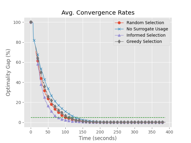
Figure 3: Convergence rates of a baseline BD, and Surrogate-MP with three selection methods (greedy, random, informed).

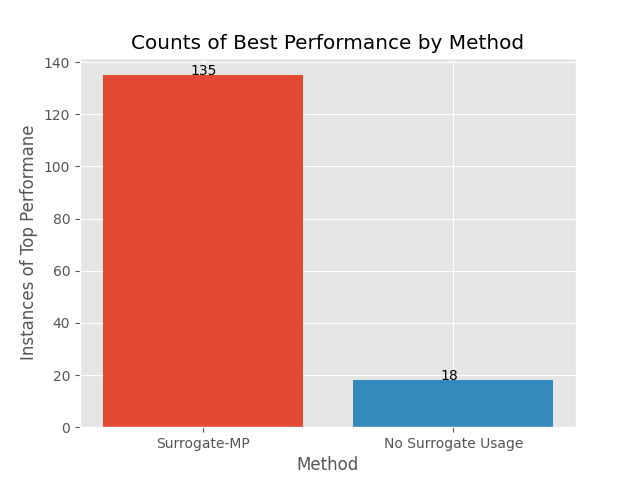
Figure 4: Count of instances with faster convergence between Surrogate-MP and a baseline BD implementation.

Acknowledging the strong performance of Surrogate-MP with informed selection, we continued our experiments by testing different frequencies of surrogate model usage. We leveraged three different rate parameters $\Gamma$ that control whether to use the surrogate model during each iteration ($[0,1]\sim\text{Bernoulli}(\Gamma)$). We experimented with $\Gamma=0.25,0.50,\text{and }0.75$. For every value of $\Gamma$ we use Surrogate-MP with informed selection. We observe in figures 5 and 6 that more frequent surrogate model usage results in improved convergence, with optimal convergence rates being generated by $\Gamma=0.75$.

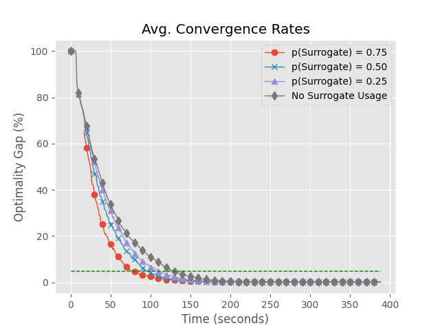
Figure 5: Convergence rates for different levels of informed surrogate usage. The dotted line indicates a gap of $5\%$ (the point at which we deactivate the Surrogate-MP).

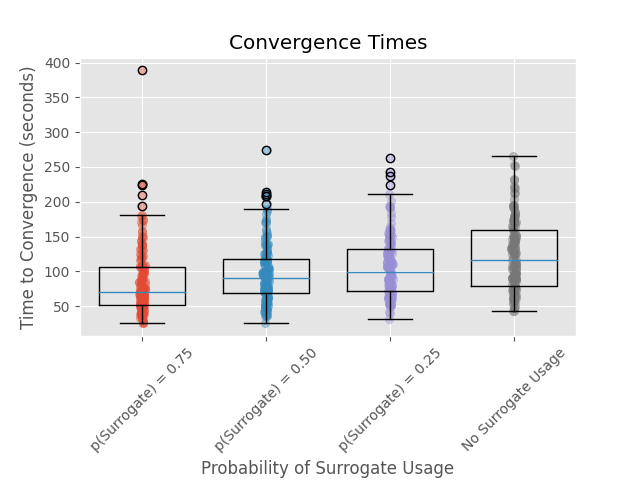
Figure 6: Convergence instances of BD accelerated by an informed Surrogate-MP, with different surrogate usages.

7 Conclusion & Future Work

In conclusion, by inserting a surrogate model in place of the MIMP we achieve a drastic reduction in convergence time. The proposed method is generalizable to any BD implementation, retreives certificates of optimality, and any surrogate capable of generating MP solutions can be used. We leverage an RL agent as our surrogate, and display results showing superiority in $88.24\%$ of instances with a $30\%$ reduction in average run time.

Observing the performance of our method, a promising extension of this work would be to design stronger integration between the surrogate model, SP, and MP. We took steps toward integration with the informed method of selecting surrogate solutions, and realized promising results. Some opportunities for integration we leave unexplored would be to directly inform the surrogate model on the strength of past solutions, offer sub-gradient information as a feature, or redesign the surrogate objective function to focus on weakly approximated areas of the SP loss as opposed to mirroring the BD objective directly. We are additionally eager to observe the performance of Surrogate-MP on other discrete SO problems.

Disclaimer.

This paper was prepared for informational purposes by the Artificial Intelligence Research group of JPMorgan Chase & Co. and its affiliates (“JP Morgan”), and is not a product of the Research Department of JP Morgan. JP Morgan makes no representation and warranty whatsoever and disclaims all liability, for the completeness, accuracy or reliability of the information contained herein. This document is not intended as investment research or investment advice, or a recommendation, offer or solicitation for the purchase or sale of any security, financial instrument, financial product or service, or to be used in any way for evaluating the merits of participating in any transaction, and shall not constitute a solicitation under any jurisdiction or to any person, if such solicitation under such jurisdiction or to such person would be unlawful.

References

- Adulyasak et al. [2015] Yossiri Adulyasak, Jean-François Cordeau, and Raf Jans. Benders decomposition for production routing under demand uncertainty. Operations Research, 63(4):851–867, 2015. doi: 10.1287/opre.2015.1401. URL https://doi.org/10.1287/opre.2015.1401.
- Arslan et al. [2021] Ayşe N Arslan, Walid Klibi, and Benoit Montreuil. Distribution network deployment for omnichannel retailing. European Journal of Operational Research, 294(3):1042–1058, 2021.
- Baena et al. [2020] Daniel Baena, Jordi Castro, and Antonio Frangioni. Stabilized benders methods for large-scale combinatorial optimization, with application to data privacy. Management Science, 66(7):3051–3068, 2020. doi: 10.1287/mnsc.2019.3341. URL https://doi.org/10.1287/mnsc.2019.3341.
- Crainic et al. [2016] Teodor Gabriel Crainic, Mike Hewitt, Francesca Maggioni, and Walter Rei. Partial benders decomposition strategies for two-stage stochastic integer programs. 2016.
- Delarue et al. [2020] Arthur Delarue, Ross Anderson, and Christian Tjandraatmadja. Reinforcement learning with combinatorial actions: An application to vehicle routing. Advances in Neural Information Processing Systems, 33:609–620, 2020.
- Gendreau et al. [1996] Michel Gendreau, Gilbert Laporte, and René Séguin. Stochastic vehicle routing. European journal of operational research, 88(1):3–12, 1996.
- Ghodrati et al. [2013] Ahmadreza Ghodrati, Hassan Abyak, and Abdorreza Sharifihosseini. Atm cash management using genetic algorithm. Management Science Letters, 3(7):2007–2041, 2013.
- Goel and Gutierrez [2011] Ankur Goel and Genaro J Gutierrez. Multiechelon procurement and distribution policies for traded commodities. Management Science, 57(12):2228–2244, 2011.
- Lee et al. [2021] Mengyuan Lee, Ning Ma, Guanding Yu, and Huaiyu Dai. Accelerating generalized benders decomposition for wireless resource allocation. IEEE Transactions on Wireless Communications, 20(2):1233–1247, 2021. doi: 10.1109/TWC.2020.3031920.
- Poojari and Beasley [2009] C.A. Poojari and J.E. Beasley. Improving benders decomposition using a genetic algorithm. European Journal of Operational Research, 199(1):89–97, 2009. ISSN 0377-2217. doi: https://doi.org/10.1016/j.ejor.2008.10.033. URL https://www.sciencedirect.com/science/article/pii/S0377221708009740.
- Schulman et al. [2017] John Schulman, Filip Wolski, Prafulla Dhariwal, Alec Radford, and Oleg Klimov. Proximal policy optimization algorithms. CoRR, abs/1707.06347, 2017. URL http://arxiv.org/abs/1707.06347.
- Sutton and Barto [2018] Richard S. Sutton and Andrew G. Barto. Reinforcement Learning: An Introduction. The MIT Press, second edition, 2018. URL http://incompleteideas.net/book/the-book-2nd.html.
- Sutton et al. [1999] Richard S Sutton, David McAllester, Satinder Singh, and Yishay Mansour. Policy gradient methods for reinforcement learning with function approximation. In S. Solla, T. Leen, and K. Müller, editors, Advances in Neural Information Processing Systems, volume 12. MIT Press, 1999. URL https://proceedings.neurips.cc/paper_files/paper/1999/file/464d828b85b0bed98e80ade0a5c43b0f-Paper.pdf.