Detecting Throat Cancer from Speech Signals Using Machine Learning: A Reproducible Literature Review

Abstract

In this work we perform a scoping review of the current literature on the detection of throat cancer from speech recordings using machine learning and artificial intelligence. We find 22 papers within this area and discuss their methods and results. We split these papers into two groups - nine performing binary classification, and 13 performing multi-class classification. The papers present a range of methods with neural networks being most commonly implemented. Many features are also extracted from the audio before classification, with the most common bring mel-frequency cepstral coefficients. None of the papers found in this search have associated code repositories and as such are not reproducible. Therefore, we create a publicly available code repository of our own classifiers. We use transfer learning on a multi-class problem, classifying three pathologies and healthy controls. Using this technique we achieve an unweighted average recall of 53.54%, sensitivity of 83.14%, and specificity of 64.00%. We compare our classifiers with the results obtained on the same dataset and find similar results.

Introduction

In the UK more than 2,000 people are diagnosed with laryngeal cancer each year (NHS, (2018)). Patients often present with a change in voice, painful or difficulty in swallowing, or a lump in the neck (NHS, (2018)). When patients present with these symptoms to their primary care provider they are referred on the two week wait (2WW) pathway. This means that they are referred to see a specialist within two weeks of the initial appointment with their primary care provider (Elliss-Brookes et al., (2012)). It has been found that a only 4.3 - 8.0% of patients referred on the 2WW pathway have head and neck cancer (Tikka et al., (2020)). Not only do such referrals cause stress and anxiety for patients, it could be argued that they also waste time and resources. Were patients able to be screened, the load on secondary care institutions may be eased and patients may be better served and by prioritising high risk patients appropriately. Earlier cancer diagnosis may be also be achieved.

Current diagnostic techniques include assessing the clinical history, clinicians assessment of voice, nasendoscopy, laryngoscopy, and biopsy (NHS, (2017)). Nasendoscopy is used to view the larynx using a small camera and is a standard out-patient procedure; a fibre-optic endoscope is inserted into the patient’s nose and passed into the throat to view the larynx and hypopharynx. If abnormalities are identifed then biopsies can be taken under local anaesthetic in the out-patient setting, or, by performing a laryngoscopy procedure requiring general anaesthesia. With the patient anaesthetised a comprehensive assessment of the larynx can be undertaken and biopsies performed as necessary(NHS, (2017)).

Speech assessment techniques are used to assist in the diagnosis of voice disorders and to measure the degree of abnormality. There are two main protocols commonly used. The first is the GRBAS scale. This is a reproducible clinical assessment of abnormal voice commonly used in clinical practice. Various aspects of the patient’s voice are scored on a scale of zero to three, where zero is normal, one is mild, two is moderate, and three is severe, across five different vocal elements; grade, roughness, breathiness, asthenia, and strain (Reghunathan and Bryson, (2019)). The second is the Consensus Auditory-Perceptual Evaluation of Voice (CAPE-V). This is an assessment tool which requires patients to perform three speech tasks. Six features of speech are assessed for each task - overall severity, roughness, breathiness, strain, pitch, and loudness. Each feature is rated on a scale from 0 (normal) to 100 (severe) (Kempster et al., (2009)).

Several machine learning (ML) and artificial intelligence (AI) methods have been implemented to detect throat cancer from speech recordings. Steps in the typical classification pipeline can be seen in Figure 1.

Figure 1: The classification pipeline generally used for the classification of pathological speech. Both preprocessing and feature selection are optional steps which are not performed by all papers.

In this work a scoping literature review is performed to document and analyse current machine learning and artificial intelligence methods for the classification of throat cancer verses benign pathology from speech.

1 Literature Search Criteria

1.1 Research Questions

In order to assess the current work in this field this literature review will address the research questions (RQ):

• RQ1: What machine learning and artificial intelligence algorithms have been used for the detection of vocal pathologies including throat cancer from patient speech?

• RQ2: What features of speech can be used to identify pathological speech including throat cancer?

RQ1 focuses on the identification of classification methods and RQ2 focuses on the feature extraction from patient speech.

1.2 Search Strategy

A literature search was conducted across three databases: Scopus, Web of Science, and PubMed. Search terms were discussed with both technical and clinical experts to ensure that they sufficiently covered the desired topics. The search terms can be seen in Table 1. The publication’s title, abstract, and keywords were searched using these terms.

Table 1: The search terms used in the literature review.

Cancer	Throat	Speech	Detection	Machine Learning
cancer*	throat	audio	classifi*	“machine learning”
carcinoma*	larynx	speech	diagnos*	“artificial intelligence”
tumour*	laryngeal	sound	detection	“neural networks”
tumor*	“voice box”	spectrograms		ml
neoplasm*	glottis	voice		ai
malignan*	glottic	vocal
	“vocal cord”	prosody
	supraglottis	acoustic
	supraglottic

1.3 Inclusion and Exclusion Criteria

All primary research study designs were included with review papers being excluded. Papers were excluded if they were not written in English and if a full version of the manuscript was not available.

The inclusion criteria were that the paper must:

• Specifically state that patients with throat cancer are included in their dataset.

• Use machine learning or artificial intelligence methods to classify patients with a vocal pathology.

• Use speech recordings (or features obtained from speech) as the primary input to the classification system.

1.4 Screening Process and Results

Using the search terms in Table 1 and assessment of appropriate conference procedings, relevant papers were identified. Figure 2 shows how the papers were screened.

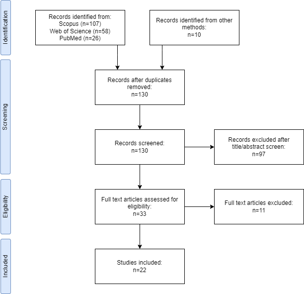
Figure 2: The Prisma diagram showing the steps taken to obtain relevant papers for this literature search.

1.5 Data Collection and Analysis

From each paper we extracted:

• The source and full reference.

• Any preprocessing steps performed.

• The features used in classification.

• The classification methods used.

• The results obtained.

The papers were grouped into two distinct types - those which performed binary classification, and those which performed multi-class classification.

2 Literature Review Results and Analysis

2.1 Results Summary

From our searches 130 papers were found. We first performed a title screening which excluded 91 papers. We then attempted to access the papers, we were unable to access 3. We assessed the abstracts of the remaining papers and excluded a further 3. During the full text screening 10 papers were rejected, 1 was a review paper, 2 did not use audio data, and 8 did not specifically state that cancer patients were included in their dataset. Of the remaining 22 papers 9 performed binary classification and 13 multi-class classification.

The results of the data extraction can be seen in Tables 2 and 3. Table 2 contains the results for the nine binary classification papers, while Table 3 contains the results for the 13 multi-class classification papers. The most common evaluation metrics used in the papers were accuracy, sensitivity, and specificity, as well as unweighted average recall (UAR) for the multi-class classification. In the below tables these metrics are listed (the best results attained in each paper). Each of these metrics is explained in more detail in Section 2.3.

Paper	Preprocessing	Features	Classification Method(s)	Accuracy	Sensitivity	Specificity
Hyun Bum Kim et al., (2020)	Normalization	Acoustic features MFCC	SVM XGBoost LightGBM ANN CNN (1D and 2D)	85.2	78.0	93.3
Wang et al., (2022)	X	MFCC	DNN	86.11	77.78	88.89
Godino-Llorente and Gomez-Vilda, (2004)	Antialiasing filter Windowing Endpoint detection	MFCC	MLP LVQ	96	94.90	95.89
Ezzine et al., (2016)	X	Glottal Parameters	MLP	98	X	X
Fang et al., 2019a	X	MFCC	DNN GMM SVM	99.14	X	X
Ben Aicha and Ezzine, (2016)	X	Glottal Parameters	ANN	96.9	X	X
Ritchings et al., (1999)	X	Fast Fourier transform	MLP	X	X	X
Gavidia-Ceballos and Hansen, (1996)	Wiener filter	Spectral features Acoustic features	HMM	90.75	X	X
Kwon et al., (2022)	X	MFCC	CNN Decision tree	87.88	94.12	81.25

Table 2: A summary of the papers found that performed binary classification. MFCC - Mel-frequency cepstral coefficients, SVM - support vector machine, XGBoost - extreme gradient boosting, LightGBM - light gradient-boosting machine, ANN - artificial neural network, CNN - convolutional neural network, DNN - deep neural network, MLP - multi-layered perceptron, LVQ - learning vector quantization, GMM - Gaussian mixture models, HMM - hidden Markov model

Paper	Preprocessing	Features	Classification Method(s)	Accuracy	Sensitivity	Specificity	UAR
Grzywalski et al., (2018)	Low-pass filtering Cropping Data augmentation	MFCC Acoustic features	DNN	X	89.4	66.0	71.2
Miliaresi et al., (2021)	Normalization Segmentation	MFCC Acoustic features Medical records	NN	57	X	X	X
Fang et al., 2019b	X	Medical records MFCC	DNN	87.26	X	X	81.59
Verikas et al., (2010)	X	Medical records Acoustic features Cosine transform coefficients	SVM	92.70	X	X	X
Ju et al., (2018)	Endpoint detection	Acoustic features MFCC Spectral features	MIL SVM Label propagation Transductive SVM	X	X	X	60.67
Islam et al., (2018)	Segmentation	Prosodic features MFCC Acoustic features	DBN SVM	X	94.9	20	59.77
Arias-Londoño et al., (2018)	Voice activity detection Normalization	Perturbation features MFCC Spectrum features Complexity features	GMM GBT SVM k-nn RF	X	92	54	61
Pham et al., (2018)	Endpoint detection	MFCC	SVM RF k-nn Gradient Boosting	68.48	X	X	X
Chuang et al., (2018)	X	MFCC	DNN	X	93.1	46	62.87
Bhat and Kopparapu, (2018)	X	Acoustic features MFCC Spectral features	BayesNet RF	X	96.6	66	68.67
Ramalingam et al., (2018)	X	Spectral features MFCC Time domain features	CNN RNN	93	96	18	X
Pishgar et al., (2018)	X	MFCC	SVM	X	88.60	78.23	59.00
Degila et al., (2018)	X	MFCC	SVM RF NN LR	X	89.4	54.0	71.30

Table 3: A summary of the papers found that performed multi-class classification. MFCC - Mel-frequency cepstral coefficients, DNN - deep neural network, NN - neural network, SVM - support vector machine, MIL - multi-instance learning, DBN - deep belief network, GMM - Guassian mixture model, GBT - gradient boosting tree, k-nn - k nearest neighbour, RF - random forest, LR - linear regression

Table 4 shows the number of cancer patients, healthy patients, and patients with non-cancer pathologies. The paper with the largest dataset is Ezzine et al., (2016) however within their work it is unclear how they obtain the number of samples from the dataset they use. The next largest dataset is Kwon et al., (2022) with 491 total patients.

Paper	Cancer	Healthy	Non-Cancer Pathology(s)
Hyun Bum Kim et al., (2020)	50	45	0
Wang et al., (2022)	43	0	129
Godino-Llorente and Gomez-Vilda, (2004)	3	53	79
Ezzine et al., (2016)	3009	3009	0
Fang et al., 2019a	48	60	354
Ben Aicha and Ezzine, (2016)	101	$>$100	0
Ritchings et al., (1999)	20	20	0
Gavidia-Ceballos and Hansen, (1996)	20	10	0
Kwon et al., (2022)	176	33	282
Grzywalski et al., (2018)	40	50	110
Miliaresi et al., (2021)	50	200	0
Fang et al., 2019b	84	0	173
Verikas et al., (2010)	22	25	193
Ju et al., (2018)	40	50	110
Islam et al., (2018)	40	50	110
Arias-Londoño et al., (2018)	40	50	110
Pham et al., (2018)	40	50	110
Chuang et al., (2018)	40	50	110
Bhat and Kopparapu, (2018)	40	50	110
Ramalingam et al., (2018)	40	50	110
Pishgar et al., (2018)	40	50	110
Degila et al., (2018)	40	50	110

Table 4: Dataset summary for each of the papers reviewed.

The classification methods used across the papers vary widely. However, neural networks and support vector machine (SVM) are the most widely used across all of the papers. Figure 3 shows the breakdown of the classification methods used in the papers. For clarity any method used only once was combined into the ‘other’ category. All neural network types were also combined into one category.

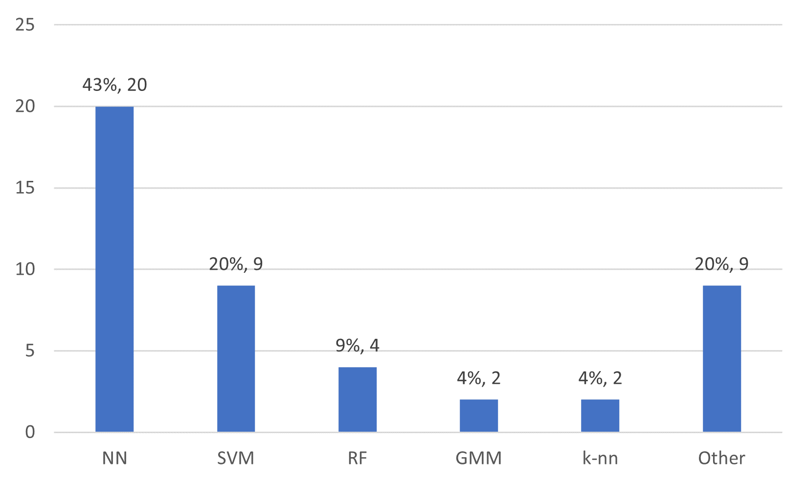
Figure 3: The classification methods used across all papers found in this review. The different neural network methods (ANN, BayesNet, CNN, DBN, DNN, LVQ, MLP, NN, RNN) were grouped and any method used only once was put into the other category for ease of visualisation. NN - neural network, SVM - support vector machine, RF - random forest, GMM - Gaussian mixture model, k-nn - k-nearest neighbour.

The features used across the papers vary greatly but the most widely used feature is Mel-frequency cepstral coefficients (MFCCs). Acoustic features is a category that contains many varied features. Generally acoustic features are those which are extracted directly from the speech signal without transforms taking place. These features are often derived from the signal’s fundamental frequency and can include jitter, shimmer, and harmonic features. Any feature used in only one paper was added to the ‘other’ category. Figure 4 shows the breakdown of features used across the papers.

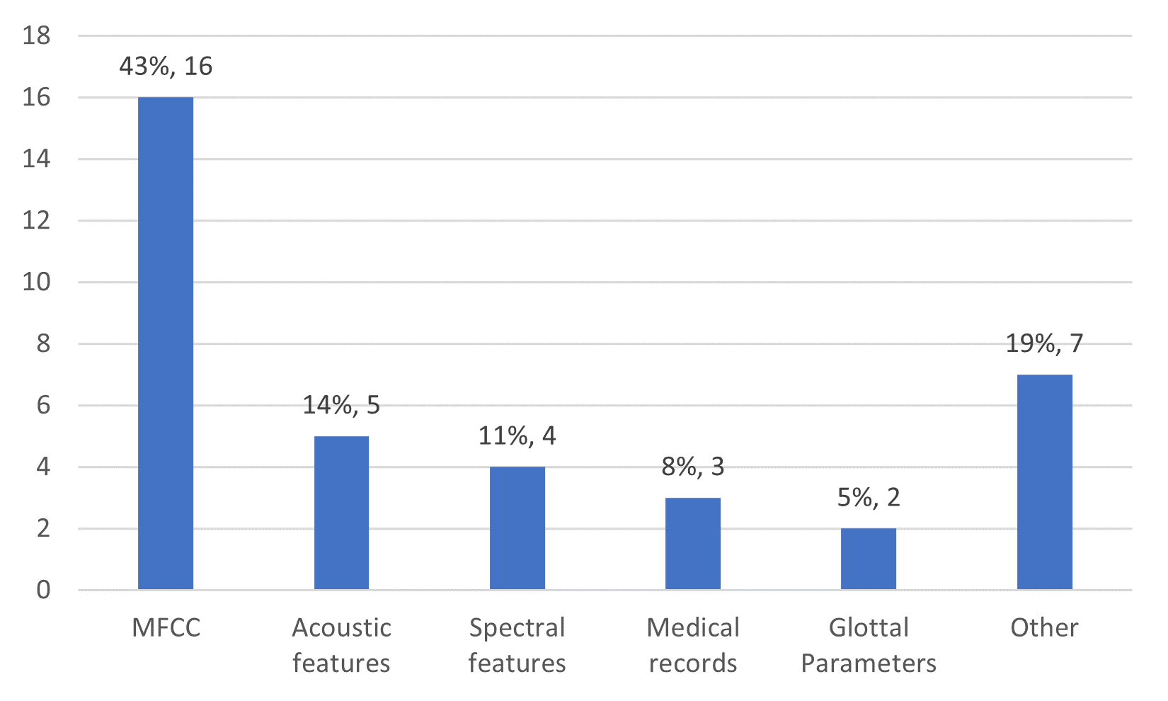
Figure 4: The features used across all papers found in this review. Any feature used only once was put into the other category for ease of visualisation. MFCC - Mel-frequency cepstral coefficients.

2.2 Features

The most common feature extracted from speech signals is Mel-frequency cepstral coefficients (MFCCs). The extraction method for MFCCs is explained in further detail below.

2.2.1 Mel-Frequency Cepstral Coefficients

The most common feature used in this literature is Mel-Frequency Cepstral Coefficients (MFCCs). Mel-Frequency refers to the Mel-scale which maps frequencies into human perception. Humans do not perceive pitch in a linear fashion, it’s easier to hear the differences between low pitches than high pitches. Figure 5 shows the conversion from frequency to the Mel scale.

Figure 5: The Mel scale - the perceptual scale of pitches.

Creating MFCCs uses fast Fourier transforms (FFTs) to transform signals from a time domain to a frequency domain. A cepstrum is defined as ”the power spectrum of the logarithm of the power spectrum” (Randall, (2017)). When creating MFCCs the audio must first be split into small overlapping sections and windowed (typically the Hanning function is applied). The FFT is then used to create magnitude spectrums for each window, these magnitude spectrums are then passed through Mel filter banks to generate Mel spectrums. Finally the discrete cosine transform is applied to produce the cepstral coefficients (Rao and K E, (2017)). Figure 6 shows the result of extracting MFCC from a speech signal.

(a) Signal of a person saying a short phrase.

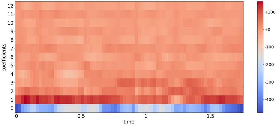
(b) MFCC generated from the above speech signal.

Figure 6: MFCCs generated from a short audio signal.

2.3 Metrics

Three metrics were widely used across the papers: accuracy, specificity, and sensitivity. The equations for these four metrics can be seen below.

$$\text{Accuracy}=\frac{\text{Correctly classified speech}}{\text{Total speech samples}}$$ (1)

$$\text{Specificity}=\frac{\text{Correctly classified healthy speech}}{\text{Total healthy speech}}$$ (2)

$$\text{Sensitivity}=\frac{\text{Correctly classified pathological speech}}{\text{Total pathological speech}}$$ (3)

Another metric was often used in the papers using multi-class classification - unweighted average recall (UAR). This metric is calculated by averaging the recall value for each of the specific pathologies included in the dataset. Equation 4 shows how it is calculated, where N is the number of pathologies in the dataset and $R_{i}$ is the recall of the ith pathology in the dataset.

$$\text{UAR}=\frac{\sum_{i=1}^{N}{R_{i}}}{N}$$ (4)

2.4 Binary Classification Literature

Hyun Bum Kim et al., (2020) investigate the classification of cancer patients from healthy controls using six machine learning algorithms. The dataset used includes recordings of the prolonged vowel /ah/ from 50 male laryngeal cancer patients and 45 male healthy controls. From these recordings 14 acoustic features were extracted as well as MFCCs. The methods used for classification are support vector machine (SVM), extreme gradient boosting (SGBoost), light gradient boosted machine (LightGBM), artificial neural network (ANN), one-dimensional convolutional neural network (1D-CNN), and two-dimensional convolutional neural network (2D-CNN). The best algorithm was found to be the 1D-CNN which took the raw signal as input, achieving an accuracy of 85.2%, sensitivity of 78.0%, and specificity of 93.3%. The performance of these models was compared to four human raters, two experts and two non-experts. The highest human accuracy was 70.9% which is outperformed by the LightGBM, 1D-CNN, and 2D-CNN.

Wang et al., (2022) classify cancer patients from patients with benign voice disorders using a deep neural network. The dataset used contains recordings of 43 cancer patients and 129 patients with benign voice disorders saying /a/. From these recordings MFCCs are extracted. The classifier achieved an accuracy of 86.11%, sensitivity of 77.78%, and specificity of 88.89% which was compared to the accuracy of two speech and language pathologists who achieved accuracies of 63% and 52%. In this work the non-cancer group was matched to the cancer group for age and sex to avoid the effects of the predominately elderly male cohort common in throat cancer, Wang et al., states that the misclassified instances are patients with smaller lesions and does not mention that patient age or gender effected the misclassification.

Godino-Llorente and Gomez-Vilda, (2004) use two deep learning methods to distinguish between healthy and pathological patients. The dataset contains 53 healthy controls and 82 pathological patients with 19 different pathologies. Within the dataset there are three patients with carcinoma. The dataset has recordings of each patient producing a sustained phonation of the vowel /ah/. From these recordings MFCCs are extracted to be used for classification. The number of MFCCs used is varied across tests, however there is no significant change in accuracy observed when this number is changed. The two deep learning methods used are multilayer perceptron (MLP) and learning vector quantization (LVQ). For these methods the number of nodes in the hidden layer (for MLP) and Kohonen layer (for LVQ) are varied. The LVQ performed significantly better than the MLP with the best model achieving 94.90% sensitivity and 95.89% specificity, although the results of the MLP are not specifically stated. The LVQ trains faster than the MLP, however, it is a larger network. Although the sensitivity and specificity achieved are impressive, there is no discussion of how well individual pathologies are classified and since some pathologies have very low numbers within the dataset, they may not appear in the test set and so the evaluation metrics may not take them into account.

Ezzine et al., (2016) use a neural network to classify speech from patients with a vocal pathology from healthy controls. The authors report 3009 healthy and 3009 cancer observations from Saarbrcker Stimmdatenbank pronouncing /a/. However, within the dataset there are only recordings available for 38 cancer patients it’s unclear how the observations were obtained. The glottal wave flow is extracted using iterative adaptive inverse filtering based on discrete all pole modelling. From the glottal wave flow several temporal and frequency descriptors were extracted. Feature selection was carried out using the distance between quartiles and correlation coefficient. The 13 optimal features were input into a multi-layered perceptron to classify the samples as cancerous or healthy. The best accuracy achieved is 98%.

Fang et al., 2019a () compares the performance of three machine learning methods to distinguish healthy and pathological patients. The dataset used includes 60 healthy controls and 402 patients with eight different pathologies, 48 of whom have a neoplasm. The subjects were recorded saying the prolonged vowel /ah/. MFCCs are extracted from these recordings as well as velocity features. The three methods used are deep neural network (DNN), support vector machine (SVM), and Gaussian mixture models (GMM). The best performance was found using a DNN with normalised MFCC and velocity features. The accuracy between male and female subjects is compared and for male subjects the accuracy is 94.26% whereas for female subjects the accuracy is only 90.52%. This is suggested to be caused by female subjects having a wider distribution in MFCC values when compared to male subjects. These models have also been validated on an external dataset and achieve similar accuracy (DNN with normalised MFCC and velocity features: 90.52%). However, on this external dataset the best performance is found using a DNN without the velocity features (99.14%). This difference is suggested to be caused by differing recording environments between the datasets, with the external dataset being recorded by a higher quality microphone in a more controlled, quieter environment. If this is the case this model would not be implementable as it’s not robust to background noise and low quality recording devices likely to be present in real world applications.

Ben Aicha and Ezzine, (2016) classify cancer patients from healthy controls using multi-layer perceptron (MLP). The dataset includes 101 utterance from cancer patients and over 100 utterances from healthy controls. From these utterances the glottal flow estimation was extracted and from this estimate temporal and frequency descriptors are calculated. An MLP is created taking each of the 14 extracted descriptors. The best accuracy is acheived using $T_{m}ax$ which is relative the maximum glottal flow. This method achieved an accuracy of 96.9%.

Ritchings et al., (1999) use a multilayer perceptron (MLP) to classify 20 male laryngeal cancer patients from 20 healthy controls. The participants were recorded saying the vowel sounds /i/ and /æ/ for up to three seconds. There is little detail about the feature extraction or construction of the MLP. It appears that the audio was framed, a fast Fourier transform was applied, and the fundamental and first five harmonics extracted. No specific performance metrics are given for the MLP just that this work “provides an improved classification of voice quality over earlier work where frequency components across the entire frequency range were used”.

Gavidia-Ceballos and Hansen, (1996) use hidden Markov models to differentiate vocal fold cancer patients from healthy controls. The dataset contains recordings of each of the 10 healthy patients and 20 vocal fold cancer patients sustaining the sound /e/ three times. From these recordings three features were extracted enhanced-spectral-pathology component, mean-area-peak-value, and weighted-slope. The best classifier used the enhanced-spectral-pathology component and achieved accuracy of 92.8% for the healthy participants and 88.7% for the cancer patients.

Kwon et al., (2022) use a combination of CNNs and decision tree to detect laryngeal cancer from speech. Within this paper laryngeal images are also used to detect cancer but in this review we only discuss the use of speech. Speech from a total of 431 patients were used in this work 176 of which have cancer and 255 which do not. The non-cancer patients consisted of patients with no pathology, cysts, palsy, edema, polyp, nodule, and other pathologies. Each patient was recorded pronouncing the vowel /a/ for at least 4 seconds. From the speech MFCCs were extracted and used as input to a CNN the best single CNN gave an accuracy of 81.08%, sensitivity of 68.97%, and specificity of 88.89%. Multiple CNNs were combined using a classification and regression tree which increased the accuracy to 87.88%, sensitivity to 94.12%, and specificity to 81.25%.

It is hard to compare the performance achieved in these papers since they use varying datasets and do not have available code to replicate their experiments. There is no clear advantage to using neural networks when compared to other machine learning methods. There is also no clear difference based on the features extracted.

2.5 Multiclass Classification Literature

Many of the papers that presented multiclass classification problems were a part of the IEEE FEMH Voice Data Challenge 2018. Therefore, we summarise the dataset used in this challenge before exploring the approaches used in these papers. Papers that conducted muticlass classification that were not a part of the challenge are detailed in Section 2.5.2.

2.5.1 IEEE FEMH Voice Data Challenge 2018

Fang et al., 2019b () present the Far Eastern Memorial Hospital (FEMH) dataset containing 589 samples and 3 pathologies: 99 neoplasm, 366 phonotrauma, and 124 vocal paralysis. In this paper the recordings of the prolonged vowel /a/ and the participant’s medical records were used to classify patients from this dataset into their specific pathologies. The medical records give 34 variables including age, gender, duration of dysphonia, symptoms, smoking and drinking habits, and a self-rating of their voice quality. From the recordings MFCCs were extracted, and the medical records were encoded. Two types of deep neural network (DNN) were created for the classification task. The first combined the MFCC and medical record features using Gaussian mixture models, this was then input into a DNN. The second used a two stage DNN, two DNNs were built, one taking the MFCC as input and the other the encoded medical record, the outputs of these DNNs were then taken as input for the final DNN which made the prediction. The highest accuracy was achieved by the two stage DNN which had an accuracy of 87.26% when differentiating between the three pathologies. The sensitivity for each of the individual classes is given, phonotrauma has a sensitivity of 95.36% which is higher than that of the neoplasm and vocal palsy classes (79.00% and 70.40% respectively) this is possibly due to the imbalance present in this dataset with there being more than three times the number of phonotrauma samples than neoplasm and almost three times the number of vocal paralysis samples.

The dataset presented by Fang et al., 2019b was used to create the IEEE FEMH Voice Data Challenge 2018. Participants were provided with 200 samples with a class breakdown shown in Table 5 to be used in training. The participant’s models were then tested on an undisclosed test set which included 50 normal, 50 neoplasm, 230 phonotrauma, and 70 vocal palsy patients.

	Neoplasm	Phonotrauma	Vocal Palsy	Healthy
Male	32	13	33	20
Female	8	47	17	30
Total	40	60	50	50

Table 5: The gender breakdown of the data provided to the challenge participants.

Ten entries to this competition were published. These ten papers are discussed below

Grzywalski et al., (2018) expanded the FEMH dataset using augmentation, for each of the pre-processed recordings three data augmentations were applied: a volume level change, a pitch shift, and a time stretch. These augmentations were applied using a random scale factor within a range. These augmentations created a training set with a total of 852 samples. Two types of feature extraction are used in this work. The first is extracting MFCCs from the recordings, the second extracted a set of acoustic features. Four types of jitter were calculated as well as the fundamental frequency and harmonics to noise ratio. The turbulent noise index and normalized first harmonic energy were also extracted. A deep neural network with two hidden layers was built and achieved a sensitivity of 89.4% and specificity of 66.0%. These measures are based on classifying pathological and healthy, not identifying which of the three pathologies the participant has. The unweighted average recall (UAR) was used to measure the model’s ability to distinguish between the three pathologies and the model had a 71.20% UAR.

Ju et al., (2018) created a pipeline of binary classifiers in which the samples are first classified into normal or pathological. Then if a sample is classified as pathological it is classified as vocal palsy or not, if the sample is not classified as vocal palsy it is then classified as either phonotrauma or neoplasm. At each stage of the pipeline the samples are classified using ensemble classifiers. The ensemble classifiers use a mixture of supervised, semi-supervised, and multiple instance learning. One supervised method was used - support vector machine (SVM), two semi-supervised methods were used - label propagation (LP) and transductive SVM, and one multiple instance methods was used - multiple-instance logistic regression (MI/LR). The MI/LR classifier had a very high AUC and so samples were labeled as positive if the probability output from the MI/LR was above 0.85 and labelled as negative if the probability was below 0.15. If the probability was between these values the sample is labelled using the majority vote of the other classifiers in the ensemble. 68 features were extracted from the signals including energy features, spectral features, MFCC, and chroma features. It was found that MFCC was the most important feature along with other features representing the signal ‘smoothness’. This approach achieved a UAR score of 60.67%.

Islam et al., (2018) use a support vector machine (SVM) to classify samples from features extracted using a deep belief network (DBN). Prosodic, vocal-tract, and excitation features are extracted from samples for a total of 54 features. Another 108 features are by taking the first and second time derivatives of each voice segment creating 162 features per segment. 15 of these segments are then concatenated making a vector of size 2430 for use in classification. The DBN was trained on the TIMIT dataset which comprises of 630 speakers of eight major dialects of American English, the dataset consists of 39 phoneme classes. Once the DBN as been trained the FEMH data is passed through it and an SVM is trained on the representations created in each layer of the DBN. The final system achieved a UAR of 59.77% with 94.90% sensitivity and 20.00% specificity.

Arias-Londoño et al., (2018) use multiple classifiers to differentiate first between normal and pathological samples, and then to differentiate the three different pathologies. Four sets of features were extracted from the samples: perturbation, spectral and cepstral, modulation spectrum, and complexity. The first classification stage is used to classify pathological and normal samples. A Gaussian mixture model (GMM) and gradient boosting tree (GBT) were used to produce scores for each sample, these scores were then fed into four classifiers: GBT, support vector machine (SVM), k-nearest neighbour (knn), and random forest (RF). The final classification is taken as the class with the highest joint probability across these four classifiers. The second classification stage takes the samples that were classified as pathological in the first stage and used one-vs-one classification with RFs trained on different subsets of features. This method achieved a sensitivity of 92%, specificity of 54% and UAR of 61%. The authors also include a confusion matrix which shows that the accuracy for each of the three pathologies is very similar (0.6 - 0.656).

Pham et al., (2018) use four machine learning methods: support vector machine (SVM), random forest (RF), k-nearest neighbor (knn), and gradient boosting (GB) to classify healthy samples and the three pathologies. The four methods were also combined using an ensemble method. MFCCs were extracted from each of the samples for input into the models. The ensemble method achieved the best accuracy of 68.48% with the best accuracy being for the healthy category and lowest for phonotrauma. Phonotrauma had the lowest accuracy across all of the methods.

Chuang et al., (2018) use a deep neural network (DNN) to both detect pathological samples from healthy samples and to detect the specific pathologies present in samples. MFCCs were extracted from the samples and taken as input to the DNN. This method achieved UAR of 62.87%, sensitivity of 93.1%, and specificity of 46%.

Bhat and Kopparapu, (2018) use a two step approach, first detecting pathological samples, and then classifying the type of pathology for each sample. For the first step of detecting pathological samples three BayesNet classifiers were trained. Each classifier classified each of samples as being healthy of one of the specific pathologies. Only samples classified as healthy by all three of the classifiers were considered healthy, all other samples continued to pathology classification. Pathology classification used a one-vs-one classification system using random forests (RF). 6552 features were extracted from the samples including MFCC, voice quality features, and spectral features. Feature selection was carried out for each of the classifiers separately and the top 20 features for each classifier selected. This method achieved UAR of 68.67%, sensitivity of 96.6%, and specificity of 66%.

Ramalingam et al., (2018) use three different neural networks for classification: multi-layer perceptron, convolutional neural network, and recurrent neural network. All three of these networks took MFCCs extracted from the samples as input as well as the MFCC deltas and simply classify smaples as healthy or pathological. The best of these models was the convolutional neural network which achieved an accuracy of 93%, sensitivity of 96%, and specificity of 18%

Pishgar et al., (2018) uses MFCCs and MFCC delta features to classify samples as being healthy or as one of the three pathologies using a support vector machine (SVM). This model achieved sensitivity of 88.60%, specificity of 78.23%, and UAR of 59.00% .

Degila et al., (2018) compare several classification methods: support vector machine (SVM), random forest, neural network, logistic regression, and ensemble methods using hard and soft voting. From the signals MFCCs with delta-delta features and MFCCs with spectral features were extracted and used as input to the classifiers. The best method was the SVM taking MFCC and spectral features as input achieving sensitivity of 89.4%, specificity of 54.0%, and UAR of 71.30%.

2.5.2 Other Multiclass Approaches

Miliaresi et al., (2021) also used the FEMH dataset but were not published as a part of the challenge. Miliaresi et al., list four pathologies, functional dysphonia, phonotrauma, laryngeal neoplasm and unilateral vocal paralysis. 50 recordings of each of the pathologies were used in training and a testing set of 200 recordings was available for testing. An undisclosed test set was used for the challenge. From the recordings MFCCs were extracted as well as three acoustic features (fundamental frequency, jitter, and harmonic to noise ratio). These features were combined with 34 medical measurements (e.g. age, gender, symptoms). The pathologies were classified using two sub-networks one taking the MFCCs as input and the other the three acoustic features and 34 medical measurements. The results of these two sub-networks were concatenated and fed into a dense layer and softmax output. This method achieved an accuracy of 57% on the undisclosed test set when differentiating between the four pathologies. In this paper there is no discussion of the difference in classification accuracies between classes. The paper recognises that the small training set is a problem with this method.

Verikas et al., (2010) use a dataset comprising of 22 cancer patients, 25 healthy patients, and 193 patients with a non-cancer pathology. The patients were asked to produce the /a/ sound for approximately two seconds, they also completed a questionnaire which gave 14 features including the patient’s age, duration of the voice disorder, and the patient’s education status. From the voice recordings 23 acoustic features were extracted as well as the average period shape, and discrete cosine transform coefficients. Two different support vector machine classifiers were built. The first exclusively used the questionnaire data. A genetic search process was used to perform feature selection and seven features were selected: age, duration of voice disorder, education level, duration of intensive speech use, cigarettes smoked per day, subjective voice function assessment by the patient, and maximum phonation time. This classifier achieved an accuracy of 92.7% when classifying the three patient groups, this classifier worked very well at differentiating the healthy and pathological patients. The second classifier used only the acoustic features extracted from the recordings and achieved an accuracy of 81.7% this model however classified many more of the patients as non-cancerous than the first model, possibly due to the imbalance in the dataset.

3 Our Contribution

None of the papers found in this review have publicly available models or code meaning that they are not reproducible. This also means that their methods and models cannot be tested externally or used by other researchers or clinicians. Therefore, we have created a publicly available repository containing the code used to create classifiers and the pretrained classifiers for a multiclass speech pathology classifier. The code and models can be found at github.com/mary-paterson/FEMH-Classification

We apply our methodology to the FEMH dataset as used in the IEEE FEMH Voice Data Challenge 2018 described in Section 2.5. We were also provided with the predictions made by each entry to the challenge as such we can directly compare our results to those made by the challenge participants. Note: the results stated in the papers presented by the participants may state slightly different results as some report results for a subset of the training data rather than the results on the unseen test data.

3.1 Methods

3.1.1 Feature Extraction

We conducted experiments using features presented in the above literature (MFCCs and acoustic features) and found that the experiments conducted using log spectrograms outperformed experiments conducted using these other features. From each recording the log spectrogram was extracted using the Python library Librosa. To obtain these spectrograms a short-time Fourier transform was applied, then scaled to remove complex numbers. The spectrogram is then displayed on a log scale. Each of the spectrograms are saved as images which are sized to 224 by 224. Figure 7 shows an example spectrogram extracted from each of the four classes.

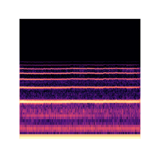
(a) Normal

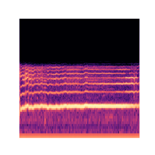
(b) Neoplasm

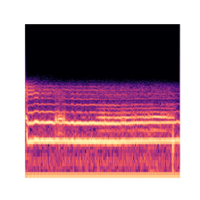
(c) Phonotrauma

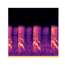
(d) Vocal palsy

Figure 7: Example spectrograms for each of the four pathologies.

3.1.2 Data Augmentation

In an attempt to improve the generalisability of our model we implemented two methods of data augmentation. First we augmented the initial training set. For each recording the pitch was shifted by a random number of steps between 0 and 0.5. Gaussian noise was then generated with a mean of 0 and standard deviation of 0.1 and added to each recording.

The second augmentation method was to add recordings from a second dataset. Recordings from the Saarbruecken Voice Database (SVD) were added to the dataset. Table 6 shows the pathologies included in each of the classes. 508 recordings from healthy patients were also added totalling 784 additional recordings for use in training.

Class	Pathologies	Number of recordings
Neoplasm	Carcinoma in situ	31
	Epiglottic cancer
	Hypopharyngeal tumor
	Larynx tumor
	Mesopharyngeal tumor
	Vocal cord cancer
Phonotrauma	Cyst	32
	Medial cervical cyst
	Phonation nodules
	Vocal fold polyp
Vocal palsy	Recurrent palsy	213
	Central-laryngeal movement disorder

Table 6: The pathologies added to the training set from the Saarbruecken Voice Database.

3.1.3 Classification

We wanted to make the implementation of our code as simple as possible, therefore, we use GoogLeNet which is widely available within libraries in both MatLab and Python.

We implemented transfer learning, using GoogLeNet to classify the audio. GoogLeNet is a 22 layer convolutional neural network Szegedy et al., (2014). GoogLeNet has been trained on ImageNet and Places365 Deng et al., (2009); Zhou et al., (2016). We edited the structure of GoogLeNet by increasing the dropout rate in the final dropout layer from 0.5 to 0.6 and replacing the output layer with a fully connected layer with an output size of four (the number of required classes). We used MatLab 2023a for the training of the models. All models were trained locally on a laptop with a Intel i7-1260P @ 2.10GHz and 16GB RAM. The models took between approximately 5 minutes and 2 hours based on the training data and model being trained.

We run four training instances using the GoogLeNet structure. The first two experiments used the pretrained GoogLeNet structure on ImageNet and Places365. We then pretrained the GoogLeNet model on the Mini Speech Commands Dataset (MSCD). The MSCD is a small excerpt of the Speech Commands Dataset (Warden, (2018)). The MSCD contains a total of 8000 recordings split equally between 8 classes (the words ’up’, ’down’, ’left’, ’right’, ’yes’, ’no’, ’go’, and ’stop’). Lastly we use the untrained GoogLeNet structure.

We used 20% of the training data as the validation set. Table 7 shows the parameters used when training the models. Early stopping was implemented such that if the validation loss does not improve over 25 validation instances training stops. The model with the lowest validation loss is saved.

Parameter	Value
Solver	SGDM
Batch Size	15
Max Epochs	200
Initial Learn Rate	1e-4
Learn Rate Drop Period	25
Learn Rate Drop Factor	0.1

Table 7: The parameters used when training the networks.

3.2 Results

Each of the models was trained on the three training datasets five times and the number of epochs and accuracy of each run recorded. Figures 8 and 9 show the mean accuracy and number of epochs for each of the training runs with the error bars corresponding to the standard deviation of the runs.

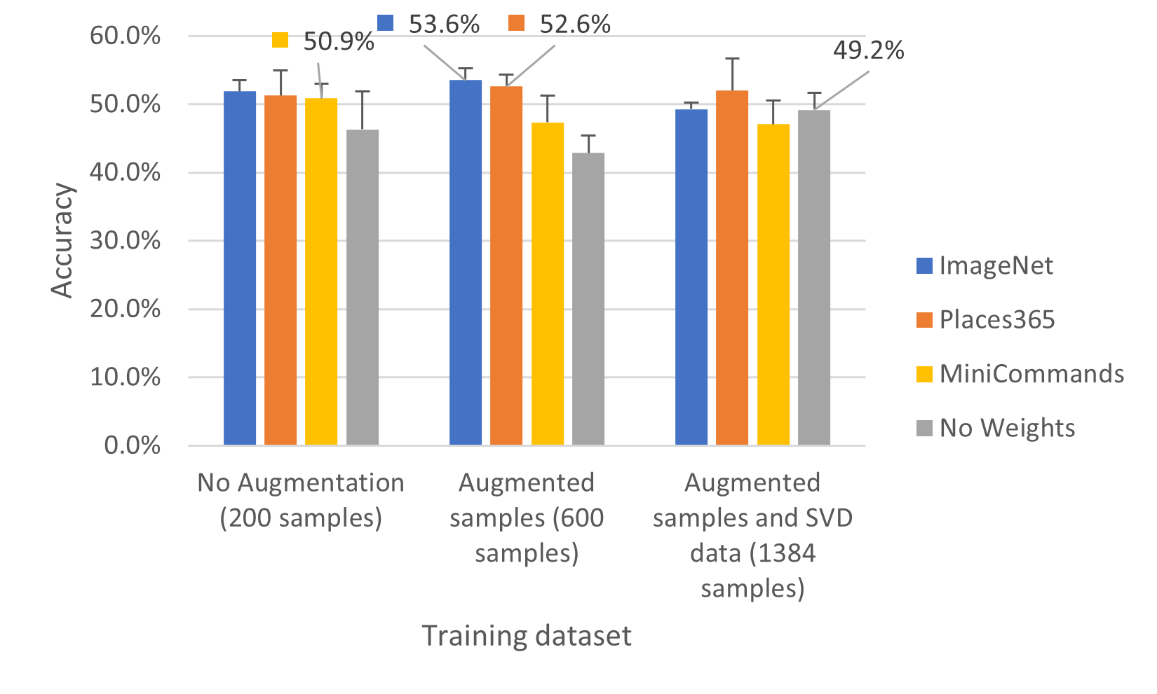
Figure 8: The accuracy of each classifier on the test set for each training dataset. The highest accuracy for each model is labelled.

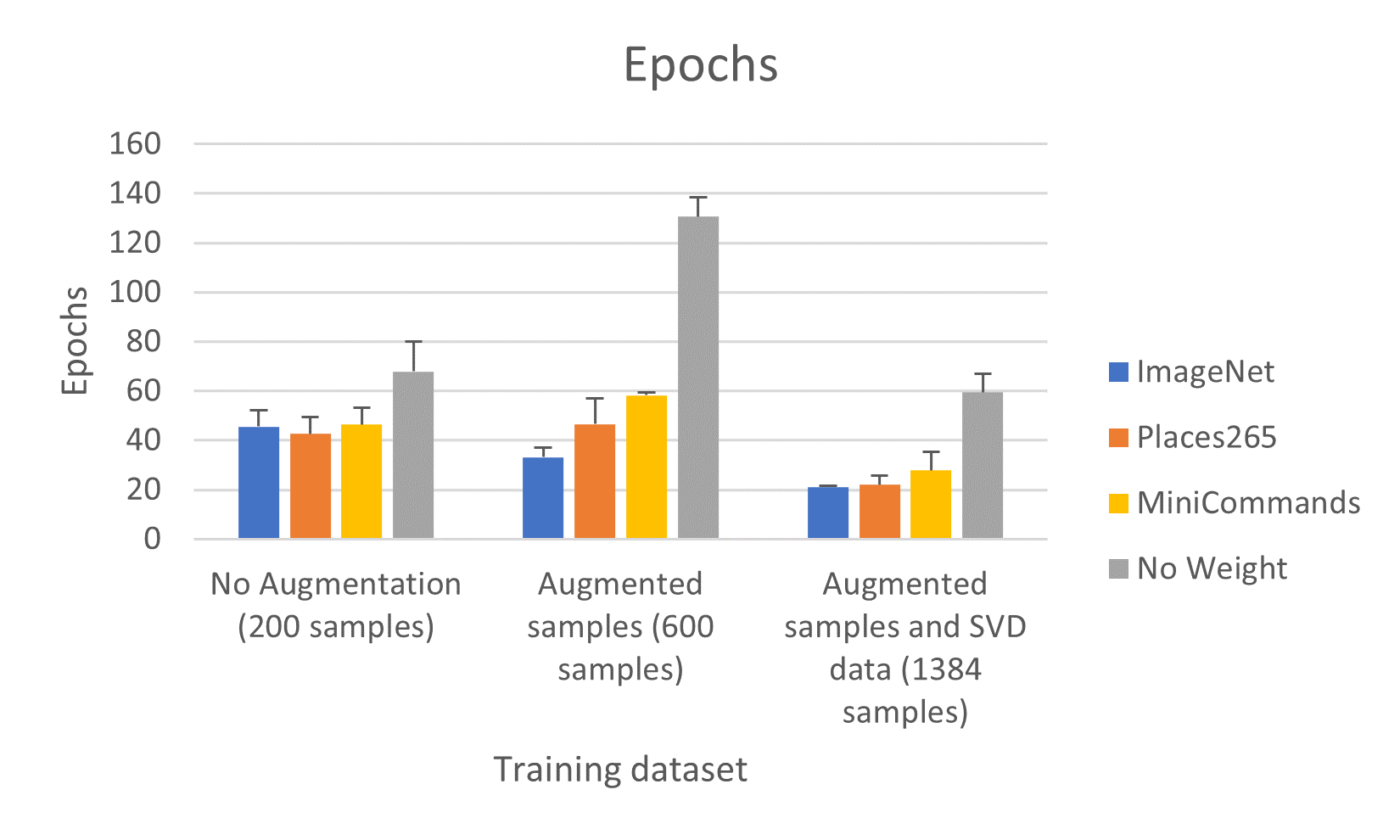
Figure 9: The epochs taken to train each classifier on each training dataset.

It can be seen in Figure 8 that the pretrained models performed considerably better than the untrained model for each of the training sets. The best average accuracy was achieved by the ImageNet model trained using the augmented dataset of 600 samples. Figure 9 also shows that the untrained model required significantly more epochs to train than the pretrained models.

The run with the highest accuracy for each model and training dataset was considered more thoroughly. For these models accuracy, specificity, sensitivity, and UAR were calculated. The equations for these metrics can be found in Section 2.3 (Equations 1, 2, 3, and 4).

Table 8 shows how each of the models performed when trained on the different training sets. The model pretrained on Places360 has a higher UAR than both of the other models although it has a generally lower specificity.

Model	Training samples	Sensitivity	Specificity	UAR
ImageNet	200	83.14%	64.00%	53.54%
	600	87.14%	54.00%	55.28%
	1384	79.14%	66.00%	49.75%
Places365	200	88.29%	32.00%	63.46%
	600	80.00%	58.00%	60.23%
	1384	82.86%	52.00%	60.61%
Mini Speech Commands	200	84.00%	54.00%	52.02%
	600	80.86%	56.00%	49.75%
	1384	73.71%	66.00%	45.84%
No Weights	200	98.57%	8.00%	46.54%
	600	72.86%	56.00%	37.76%
	1384	77.14%	40.00%	39.24%

Table 8: The results obtained by each model on the test set. The size of the training set (200 recordings in the initial training set, 600 after pitch shifting and adding noise, 1384 after adding data from the SVD) can be seen in the second column.

Figure 10 shows how we perform compared to the challenge participants. It can be seen that when using the two pretraineded models our specificity is significantly improved over the challenge participants however, this comes with a decrease in sensitivity.

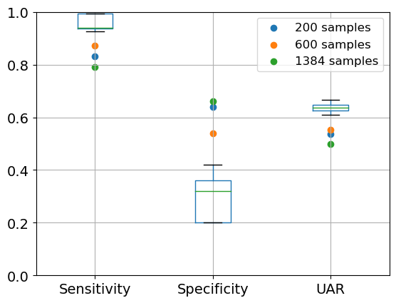
(a) ImageNet

(b) Places360

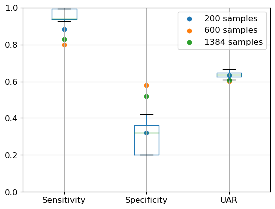
(c) Mini Speech Commands

(d) No Weights

Figure 10: Our results (the three coloured dots) compared to the challenge submissions (boxplot showing the distribution).

Conclusion

Within this scoping literature review we found 22 papers describing the classification of vocal pathologies using machine learning and speech recordings. 13 of these papers performed multi-class classification and 9 papers performed binary classification. All of these papers show that it is possible to use machine learning and artificial intelligence to detect vocal pathologies, including cancer, from speech. Varied preprocessing, feature extraction, and classification methods were used within the papers. The results of the papers vary with accuracy ranging from 85.2% to 98% for binary classification.

However, none of the papers found in this search include open source code or models and so it is not possible to recreate or verify their results. Therefore, we ran our own experiments using the dataset most commonly used in these papers and present the code and models on an open source repository such that the experiments can be recreated and verified. When comparing our results to those achieved by other authors using the same dataset we found that we significantly improved the sensitivity of the classification with a small decrease in specificity and UAR. In future work we will continue to improve the classification of vocal pathologies from speech using machine learning and artificial intelligence and freely share the code used in experiments on public repositories.

Appendix A Searches

Database	Search
Scopus	( TITLE-ABS-KEY ( cancer* OR carcinoma* OR tumour* OR tumor* OR neoplasm* OR malignan* ) ) AND ( TITLE-ABS-KEY ( throat OR larynx OR laryngeal OR ”voice box” OR glottis OR glottic OR ”vocal cord” OR supraglottis OR supraglottic ) ) AND ( TITLE-ABS-KEY ( audio OR speech OR sound OR spectrograms OR voice OR vocal OR prosody OR acoustic ) ) AND ( TITLE-ABS-KEY ( classifi* OR diagnos* OR detection ) ) AND ( TITLE-ABS-KEY ( ”machine learning” OR ”artificial intelligence” OR ”neural networks” OR ml OR ai ) ) AND ( LIMIT-TO ( LANGUAGE , ”English” ) )
Web of Science	((((TS=(cancer* OR carcinoma* OR tumour* OR tumor* OR neoplasm* OR malignant)) AND TS=(throat OR larynx OR laryngeal OR ”voice box” OR glottis OR glottic OR ”vocal cord” OR supraglottis OR supraglottic)) AND TS=(audio OR speech OR sound OR spectrograms OR voice OR vocal OR prosody OR acoustic)) AND TS=(classifi* OR diagnos* OR detection )) AND TS=(”machine learning” OR ”artificial intelligence” OR ”neural networks” OR ml OR ai) and English (Languages)
PubMed	(((((((((cancer*[Title/Abstract]) OR (carcinoma*[Title/Abstract])) OR (tumour*[Title/Abstract])) OR (tumor*[Title/Abstract])) OR (neoplasm*[Title/Abstract])) OR (malignan*[Title/Abstract])) AND (((((((((throat[Title/Abstract]) OR (larynx[Title/Abstract])) OR (laryngeal[Title/Abstract])) OR (”voice box”[Title/Abstract])) OR (glottis[Title/Abstract])) OR (glottic[Title/Abstract])) OR (”vocal cord”[Title/Abstract])) OR (supraglottis[Title/Abstract])) OR (supraglottic[Title/Abstract]))) AND ((((((((audio[Title/Abstract]) OR (speech[Title/Abstract])) OR (sound[Title/Abstract])) OR (spectrograms[Title/Abstract])) OR (voice[Title/Abstract])) OR (vocal[Title/Abstract])) OR (prosody[Title/Abstract])) OR (acoustic[Title/Abstract]))) AND (((classifi*[Title/Abstract]) OR (diagnos*[Title/Abstract])) OR (detection[Title/Abstract]))) AND (((((”machine learning”[Title/Abstract]) OR (”artificial intelligence”[Title/Abstract])) OR (”neural networks”[Title/Abstract])) OR (ml[Title/Abstract])) OR (ai[Title/Abstract]))

Table 9: The searches used in each of the databases.