Axion dark matter with explicit Peccei-Quinn symmetry breaking in the axiverse

Abstract

It is shown that the required high quality of the Peccei-Quinn (PQ) symmetry can be a natural outcome of the multiple QCD axion models. In the axiverse, a hypothetical mass mixing between the QCD axions and axion-like particles (ALPs) can occur, which leads to an interesting phenomenon called the level crossing. In this paper, we investigate this mass mixing between one QCD axion and one ALP with the explicit PQ symmetry breaking in the early Universe. The dynamics of the axions and their cosmological evolutions when the level crossing occurs in this scenario are studied in detail. Then we focus our attention on the axion dark matter (DM) abundance. With several typical parameter sets for level crossing, we find that in the presence of the explicit PQ symmetry breaking term in the mixing, the total axion DM abundance is dominated by ALP and significantly suppressed.

1 Introduction

The nature of dark matter (DM) is a long-standing mystery in particle physics, cosmology, and astrophysics. While the axion is one of the leading DM candidates, which was predicted by the Peccei-Quinn (PQ) mechanism with a spontaneously broken global $U(1)_{\rm PQ}$ symmetry Peccei:1977ur ; Peccei:1977hh to solve the strong CP problem in the Standard Model (SM), also called the QCD axion Weinberg:1977ma ; Wilczek:1977pj ; Kim:1979if ; Shifman:1979if ; Dine:1981rt ; Zhitnitsky:1980tq . The QCD axion is a light pseudo-Nambu-Goldstone boson, which acquires a tiny mass from the QCD anomaly tHooft:1976rip ; tHooft:1976snw . When the QCD instanton generates the QCD axion potential, the axion stabilizes at the CP conservation minimum value, which solves the strong CP problem. As the DM candidate, the QCD axion can be non-thermally produced in the early Universe through misalignment mechanism Preskill:1982cy ; Abbott:1982af ; Dine:1982ah . The QCD axion is massless at high cosmic temperatures, but as the temperature decreases, it gains a non-zero mass at the QCD phase transition and begins to oscillate when the mass is comparable to the Hubble parameter, which can explain the observed cold DM abundance. The misalignment mechanism gives the upper limit of the classical axion window, $10^{9}\,{\rm GeV}\lesssim f_{a}\lesssim 10^{12}\,{\rm GeV}$, where $f_{a}$ is the QCD axion decay constant, and the lower limit is given by the SN 1987A neutrino burst duration Mayle:1987as ; Raffelt:1987yt ; Turner:1987by and the cooling of the neutron star Leinson:2014ioa ; Hamaguchi:2018oqw ; Buschmann:2021juv . However, the origin of the PQ scale at this window is still unknown, which may come from the supersymmetry (SUSY) breaking scale and the Planck scale Carpenter:2009zs ; Yin:2020dfn . In the case with $f_{a}\sim\mathcal{O}(10^{16})\,{\rm GeV}$, the axion DM abundance will be overproduced if without fine-tuning of the initial misalignment angle, which is the problem of overproduction of the axion DM.

On the other hand, the PQ mechanism relies on the high quality of the global PQ symmetry, which works when the global PQ symmetry is explicitly broken and other explicit breaking effects are highly Planck-suppressed Kamionkowski:1992mf ; Barr:1992qq ; Ghigna:1992iv . There is a sharper argument that the continuous global symmetries should not exist in the quantum gravity theory Kallosh:1995hi ; Banks:2010zn ; Harlow:2018tng ; Reece:2023czb , and the PQ mechanism can be easily spoilt by the explicit PQ breaking operators Higaki:2016yqk ; Jeong:2022kdr . From the low energy perspective, it is difficult to explain why the breaking of PQ symmetry rather than QCD is so small, which is the problem of high quality of the PQ symmetry. Therefore, it is essential to investigate the explicit PQ symmetry breaking effects and their implications, and many works are studied. We are more concerned about a case that the required high quality of the PQ symmetry is a natural outcome of the multiple QCD axion models, $\rm e.g.$, the aligned QCD axion Choi:2014rja ; Higaki:2014pja ; Higaki:2014mwa , and the clockwork QCD axion Choi:2015fiu ; Kaplan:2015fuy ; Long:2018nsl . In refs. Higaki:2016yqk ; Higaki:2015jag , they show that the high quality PQ symmetry can be naturally explained in the aligned QCD axion models with the decay constants much smaller than the classical axion window. The implications of the explicit PQ symmetry breaking on QCD axion DM are also studied in refs. Nakagawa:2020zjr ; Jeong:2022kdr . Another effect of the explicit PQ symmetry breaking is reflected in the formation of QCD axion bubbles Kitajima:2020kig ; Li:2023det ; Li:2023zyc ; Kasai:2023ofh .

Several extensions of the SM, such as string theory Green:1984sg ; Witten:1984dg , predicted the axion-like particle (ALP), which has similar properties to QCD axion but not have to solve the strong CP problem. In addition, the ALP mass and its coupling to the SM particles are not relevant, $\rm e.g.$, coupling to photon Halverson:2019cmy ; Li:2020pcn ; Cyncynates:2021xzw ; Li:2022jgi ; Li:2022pqa , which are correlative in the QCD axion. The ALP is also the DM candidate and can be produced in the early Universe through misalignment mechanism Cadamuro:2011fd ; Arias:2012az ; Chao:2022blc . The Universe with a large number of axions and ALPs is called the axiverse Svrcek:2006yi ; Arvanitaki:2009fg ; Demirtas:2021gsq . In the axiverse, the cosmological evolution called the level crossing can take place if there is a non-zero mass mixing between the QCD axions and ALPs, which are extensively studied in refs. Hill:1988bu ; Kitajima:2014xla ; Daido:2015cba ; Ho:2018qur ; Daido:2015bva ; Murai:2023xjn ; Cyncynates:2023esj . Generally, the condition for level crossing is that the zero-temperature mass and decay constant of the ALP are both much smaller than that of the QCD axion Ho:2018qur . This may induce the adiabatic transition of these axions, which is similar to the Mikheyev-Smirnov-Wolfenstein (MSW) effect Wolfenstein:1977ue ; Mikheyev:1985zog ; Mikheev:1986wj in neutrino oscillations. The adiabatic transition can lead to the suppression of the axion energy density and isocurvature perturbations Kitajima:2014xla ; Daido:2015cba ; Ho:2018qur . The axion DM from the level crossing and the coupling to photon are studied in ref. Ho:2018qur . Furthermore, the domain wall formation from the level crossing is also discussed in ref. Daido:2015bva .

In this paper, we investigate the non-zero mass mixing between the QCD axions and ALPs in the axiverse with the explicit PQ symmetry breaking in the early Universe. Exactly, we consider the mixing with one QCD axion and one ALP. The dynamics of the axions and their cosmological evolutions when the level crossing occurs in this scenario are studied in detail. With several typical parameter sets for level crossing, we show the distributions of the mass eigenvalues and mass mixing angle, and also check the condition for adiabatic transition in this scenario. Then we focus our attention on the axion DM abundance. If there is no mass mixing between the QCD axion and ALP, the QCD axion dominates the total axion DM abundance. In the presence of the explicit PQ symmetry breaking term in the mixing, the total axion DM abundance is dominated by ALP and significantly suppressed.

The rest of this paper is organized as follows. In section 2, we first review the QCD axion and ALP DM, and introduce the mass mixing between them. In section 3, we investigate the explicit PQ symmetry breaking effects on axion mass mixing in the axiverse, focusing on the dynamics of the axions and their cosmological evolutions, and also the axion DM abundance. The conclusion is given in section 4.

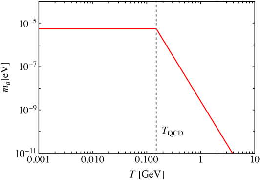
Figure 1: The temperature-dependent QCD axion mass $m_{a}(T)$ as a function of the cosmic temperature $T$ for $f_{a}=10^{12}\,{\rm GeV}$. The vertical gray line represents the temperature $T_{\rm QCD}$.

2 Axion mass mixing in the axiverse

In this section, we review the QCD axion and ALP DM produced by the misalignment mechanism, and then briefly introduce the mass mixing between them.

2.1 QCD axion and ALP dark matter

Here we consider the pre-inflationary scenario, $\rm i.e.$, the PQ symmetry is spontaneously broken during inflation. The QCD axion ($a$) effective potential $V_{\rm QCD}(\phi)$ from the QCD non-perturbative effects is given by

$$V_{\rm QCD}(\phi)=m_{a}^{2}(T)f_{a}^{2}\left[1-\cos\left(\frac{\phi}{f_{a}}\right)\right]\,,$$ (1)

where $\phi$ is the QCD axion field, $f_{a}$ is the QCD axion decay constant, $\theta=\phi/f_{a}$ is the QCD axion angle, $m_{a}(T)$ is the temperature-dependent QCD axion mass

$$m_{a}(T)\simeq m_{a,0}\left(\frac{T}{T_{\rm QCD}}\right)^{-n}\,,$$ (2)

for the cosmic temperature $T\gtrsim T_{\rm QCD}\simeq 150\,\rm MeV$ with $n\simeq 4.08$ Borsanyi:2016ksw , and $m_{a,0}$ is the zero-temperature QCD axion mass GrillidiCortona:2015jxo

$$m_{a,0}=\frac{m_{\pi}f_{\pi}}{f_{a}}\frac{\sqrt{m_{u}/m_{d}}}{1+m_{u}/m_{d}}\simeq 5.70(7)\,{\mu\rm eV}\left(\frac{f_{a}}{10^{12}\,{\rm GeV}}\right)^{-1}\,,$$ (3)

for $T<T_{\rm QCD}$, where $m_{\pi}$ and $f_{\pi}$ are the mass and decay constant of the pion, $m_{u}$ and $m_{d}$ are the up and down quark masses, respectively. Using eqs. (2) and (3), we show the QCD axion mass as a function of the cosmic temperature in figure 1 for later use.

As the cosmic temperature decreases, the QCD axion starts to oscillate when its mass $m_{a}(T)$ becomes comparable to the Hubble parameter $H(T)$, which is given by the Friedmann equation in the radiation-dominated era

$$3M_{\rm Pl}^{2}H^{2}(T)=\frac{\pi^{2}}{30}g_{*}(T)T^{4}\,,$$ (4)

where $M_{\rm Pl}$ is the reduced Planck mass, and $g_{*}$ is the number of effective degrees of freedom of the energy density. Using $3H(T_{{\rm osc},a})=m_{a}(T_{{\rm osc},a})$, then the oscillation temperature is given by

$$T_{{\rm osc},a}\simeq 0.96\,{\rm GeV}\left(\frac{g_{*}(T_{{\rm osc},a})}{61.75}\right)^{-0.082}\left(\frac{f_{a}}{10^{12}\,\rm GeV}\right)^{-0.16}\,.$$ (5)

The ratio of the QCD axion number density $n_{a}$ to the entropy density at $T_{{\rm osc},a}$ reads

$$\frac{n_{a}(T)}{s(T)}\bigg{|}_{T=T_{{\rm osc},a}}\simeq\frac{1}{2}\frac{m_{a}(T_{{\rm osc},a})}{s(T_{{\rm osc},a})}f_{a}^{2}\left\langle\theta_{i}^{2}f(\theta_{i})\right\rangle\chi\,,$$ (6)

where $s(T)=2\pi^{2}g_{*s}(T)T^{3}/45$ is the entropy density, $g_{*s}$ is the number of effective degrees of freedom of the entropy density, $\theta_{i}$ is the initial misalignment angle, $f(\theta_{i})$ is the anharmonicity factor Lyth:1991ub ; Visinelli:2009zm

$$f(\theta_{i})\simeq\left[\ln\left(\frac{e}{1-\theta_{i}^{2}/\pi^{2}}\right)\right]^{7/6}\,,$$ (7)

and $\chi\simeq 1.44$ is a numerical factor that models the temperature-dependent QCD axion mass around $T_{{\rm osc},a}$ and depends on the number of quark flavors at $T_{{\rm osc},a}$ Turner:1985si . Then the current QCD axion DM abundance is given by

$$\begin{aligned} \Omega_{a}h^{2}&=m_{a,0}\frac{n_{a}(T)}{s(T)}\bigg{|}_{T=T_{{\rm osc},a}}\frac{s(T_{0})}{\rho_{\rm crit}h^{-2}}\\ &\simeq 0.14\left(\frac{g_{*s}(T_{0})}{3.94}\right)\left(\frac{g_{*}(T_{{\rm osc},a})}{61.75}\right)^{-0.42}\left(\frac{f_{a}}{10^{12}\,\rm GeV}\right)^{1.16}\left\langle\theta_{i}^{2}f(\theta_{i})\right\rangle\,,\end{aligned}$$ (8)

where $T_{0}$ is the present CMB temperature, $\rho_{\rm crit}=3H^{2}(T_{0})M_{\rm Pl}^{2}$ is the critical energy density, and $h\simeq 0.68$ is the reduced Hubble constant. In order to explain the observed cold DM abundance, $\Omega_{\rm DM}h^{2}\simeq 0.12$ Planck:2018vyg , we have the initial misalignment angle

$$\theta_{i}\simeq 0.87\left(\frac{g_{*s}(T_{0})}{3.94}\right)^{1/2}\left(\frac{g_{*}(T_{{\rm osc},a})}{61.75}\right)^{0.21}\left(\frac{f_{a}}{10^{12}\,\rm GeV}\right)^{-0.58}\,.$$ (9)

The above misalignment mechanism can also be applied to the ALP DM. The ALP can be directly extended from the QCD axion, which may be the low-energy consequence of the string theory Green:1984sg ; Witten:1984dg . The string axiverse describes $N$ axion fields, which obtain the non-perturbative contributions to their collective potential from $M$ instantons with $M\gg N$ Arvanitaki:2009fg ; Cyncynates:2021xzw . The effective potential is given by

$$V_{A}(\psi_{1},\dots,\psi_{N})=\sum_{i=1}^{M}\Lambda_{i}^{4}\left[1-\cos\left(\sum_{j=1}^{N}\mathcal{Q}_{ij}\frac{\psi_{j}}{f_{A,j}}+\delta_{i}\right)\right]\,,$$ (10)

where $\psi$ is the ALP field, $f_{A}$ is the ALP decay constant, $\Lambda_{i}$ is the energy scale, $\mathcal{Q}_{ij}$ is the model parameter associated with the ALP charge, and $\delta_{i}$ is the constant phase. Here we consider the ALP field $\psi$ as a mass eigenstate that orthogonal to the state of QCD axion with an eigenvalue $m_{A}$ Ho:2018qur . For $N=1$ and $m_{A}=\rm const.$, the ALP DM abundance reads

$$\begin{aligned} \Omega_{A}h^{2}&=m_{A}\frac{n_{A}(T)}{s(T)}\bigg{|}_{T=T_{{\rm osc},A}}\frac{s(T_{0})}{\rho_{\rm crit}h^{-2}}\\ &\simeq 0.95\left(\frac{g_{*s}(T_{0})}{3.94}\right)\left(\frac{g_{*}(T_{{\rm osc},A})}{61.75}\right)^{-1}\left(\frac{m_{A}}{1\,\rm eV}\right)^{1/2}\left(\frac{f_{A}}{10^{12}\,\rm GeV}\right)^{2}\left\langle\theta_{i,A}^{2}f(\theta_{i})\right\rangle\,,\end{aligned}$$ (11)

where $n_{A}$ is the ALP number density, $T_{{\rm osc},A}$ is the ALP oscillation temperature that given by $3H(T_{{\rm osc},A})=m_{A}$, and $\theta_{i,A}$ is the initial misalignment angle of the ALP field.

2.2 Axion mass mixing

In this subsection, we briefly introduce the mass mixing between the QCD axion and ALP. In the axiverse, it is natural to take into account the cosmological evolution of multiple axions. In this case, the level crossing can occur if there is a hypothetical non-zero mass mixing between the QCD axions and ALPs Hill:1988bu ; Kitajima:2014xla . Here we consider the mass mixing for the minimal scenario, one QCD axion $\phi$ and one ALP $\psi$, with the following low-energy effective Lagrangian

$$\mathscr{L}=\frac{1}{2}\partial^{\mu}\phi\partial_{\mu}\phi+\frac{1}{2}\partial^{\mu}\psi\partial_{\mu}\psi-V_{\rm mix}(\phi,\psi)\,,$$ (12)

where $V_{\rm mix}(\phi,\psi)$ is the mixing potential Kitajima:2014xla

$$V_{\rm mix}(\phi,\psi)=m_{a}^{2}(T)f_{a}^{2}\left[1-\cos\left(\frac{n_{1}\phi}{f_{a}}+\frac{n_{2}\psi}{f_{A}}\right)\right]+m_{A}^{2}f_{A}^{2}\left[1-\cos\left(\frac{n_{3}\phi}{f_{a}}+\frac{n_{4}\psi}{f_{A}}\right)\right]\,,~{}~{}~{}$$ (13)

with the domain wall numbers $n_{i}$. For simplicity, one can take $n_{1}=n_{3}=n_{4}=1$ and $n_{2}=0$ to obtain the potential

$$V_{\rm mix}(\phi,\psi)=m_{a}^{2}(T)f_{a}^{2}\left[1-\cos\left(\frac{\phi}{f_{a}}\right)\right]+m_{A}^{2}f_{A}^{2}\left[1-\cos\left(\frac{\phi}{f_{a}}+\frac{\psi}{f_{A}}\right)\right]\,.$$ (14)

The dynamics and cosmological evolution of the axions in this case are studied in detail in refs. Kitajima:2014xla ; Daido:2015cba ; Ho:2018qur . In the mixing, the mass eigenvalues $m_{1}(T)$ and $m_{2}(T)$ of the mass eigenstates $a_{1}$ and $a_{2}$ would approach to each other under a certain condition, $\rm e.g.$, both the mass and decay constant of the ALP should be much smaller than the QCD axion, and then move away from each other due the cosmic temperature decreasing, which is called the level crossing. At level crossing, the adiabatic transition can occur between these two mass eigenstates when the adiabatic condition is satisfied. The final axion abundance and isocurvature perturbations can be suppressed by the adiabatic transition between them Kitajima:2014xla ; Ho:2018qur . Furthermore, the level crossing can also lead to the formation of domain wall, which is a more common phenomenon in the axiverse than previously thought Daido:2015bva . Recently, the heavy QCD axion DM from the avoided level crossing is studied in ref. Cyncynates:2023esj , in which the QCD axion mixes with the sterile axion, leading to an avoided level crossing of their mass eigenstates.

3 Effects of explicit Peccei-Quinn symmetry breaking

In this section, we investigate the effects of the explicit PQ symmetry breaking on axion mass mixing in the axiverse with one QCD axion and one ALP.

3.1 Explicit Peccei-Quinn symmetry breaking

We first briefly discuss the explicit PQ symmetry breaking effects on QCD axion DM, see ref. Jeong:2022kdr for more details. Here we consider the following explicit PQ symmetry breaking potential from the quantum gravity effects Higaki:2016yqk

$$V_{\cancel{\rm PQ}}(\phi)=m_{\cancel{\rm PQ}}^{2}f_{a}^{2}\left[1-\cos\left(N_{H}\left(\frac{\phi}{f_{a}}-\theta_{H}\right)\right)\right]\,,$$ (15)

where $m_{\cancel{\rm PQ}}$ is the corresponding effective mass, $N_{H}$ is an integer, and $\theta_{H}$ is the phase. In this case, the axion starts to oscillate when its mass becomes comparable to the Hubble parameter $H(T)$, $3H(T^{\prime}_{{\rm osc},a})=N_{H}m_{\cancel{\rm PQ}}$, with the oscillation temperature

$$T^{\prime}_{{\rm osc},a}\simeq 17.66\,{\rm GeV}\left(\frac{N_{H}}{1}\right)^{1/2}\left(\frac{g_{*}(T^{\prime}_{{\rm osc},a})}{61.75}\right)^{-1/4}\left(\frac{m_{\cancel{\rm PQ}}}{1\,\rm\mu eV}\right)^{1/2}\,.$$ (16)

Since we are more concerned about the case that the axion starts to oscillate before the conventional case, $\rm i.e.$, $T^{\prime}_{{\rm osc},a}>T_{{\rm osc},a}$, then we have the lower limit

$$m_{\cancel{\rm PQ}}>2.95\times 10^{-18}\,{\rm GeV}\left(\frac{N_{H}}{1}\right)^{-1}\left(\frac{g_{*}(T^{\prime}_{{\rm osc},a})}{61.75}\right)^{0.34}\left(\frac{f_{a}}{10^{12}\,\rm GeV}\right)^{-0.33}\,.$$ (17)

Using eq. (3), we also have the relation

$$\frac{m_{\cancel{\rm PQ}}}{m_{a,0}}>5.17\times 10^{-4}\left(\frac{N_{H}}{1}\right)^{-1}\left(\frac{g_{*}(T^{\prime}_{{\rm osc},a})}{61.75}\right)^{0.34}\left(\frac{f_{a}}{10^{12}\,\rm GeV}\right)^{0.67}\,.$$ (18)

For simplicity, we consider a case with $|\theta_{i}-\theta_{H}|<\pi/N_{H}$. The QCD axion DM abundance in this case is given by

$$\begin{aligned} \Omega_{a}h^{2}&\simeq 5.40\times 10^{-3}\left(\frac{N_{H}}{1}\right)^{-1/2}\left(\frac{g_{*s}(T_{0})}{3.94}\right)\left(\frac{g_{*}(T^{\prime}_{{\rm osc},a})}{61.75}\right)^{-1/4}\left(\frac{m_{\cancel{\rm PQ}}}{1\,\rm\mu eV}\right)^{-1/2}\\ &\times\left(\frac{f_{a}}{10^{12}\,\rm GeV}\right)\left\langle\left(\theta_{i}-\theta_{H}\right)^{2}f^{\prime}(\theta_{i})\right\rangle\,,\end{aligned}$$ (19)

with the anharmonicity factor Lyth:1991ub ; Visinelli:2009zm ; Jeong:2022kdr

$$f^{\prime}(\theta_{i})\simeq\left[\ln\left(\frac{e}{1-\left(\theta_{i}-\theta_{H}\right)^{2}/\left(\pi/N_{H}\right)^{2}}\right)\right]^{3/2}\,.$$ (20)

A more complicated case with $|\theta_{i}-\theta_{H}|>\pi/N_{H}$ is also discussed in ref. Jeong:2022kdr , in which the trapping effect on QCD axion DM abundance and isocurvature perturbations is significant, depending on around which vacuum the axion first starts to oscillate.

3.2 Effects on axion mass mixing in the axiverse

Here we investigate the effects of the above explicit PQ symmetry breaking on axion mass mixing in the axiverse. In this case, the axion mixing potential is given as follows with the notation

$$V_{\rm mix}(\phi,\psi)\to V^{\prime}_{\rm mix}(\phi,\psi)+V_{\cancel{\rm PQ}}(\phi)\,.$$ (21)

Using eq. (15), we derive the mixing potential in this model

$$\begin{aligned} V_{\rm mix}(\phi,\psi)&=m_{a}^{2}(T)f_{a}^{2}\left[1-\cos\left(\frac{\phi}{f_{a}}\right)\right]+m_{\cancel{\rm PQ}}^{2}f_{a}^{2}\left[1-\cos\left(N_{H}\left(\frac{\phi}{f_{a}}-\theta_{H}\right)\right)\right]\\ &+m_{A}^{2}f_{A}^{2}\left[1-\cos\left(\frac{\phi}{f_{a}}+N_{H}\left(\frac{\phi}{f_{a}}-\theta_{H}\right)+\frac{\psi}{f_{A}}\right)\right]\,.\end{aligned}$$ (22)

Substituting eq. (22) into the equations of motion (EOM)

$$\ddot{\phi}+3H\dot{\phi}+\frac{\partial V_{\rm mix}(\phi,\psi)}{\partial\phi}=0\,,\quad\ddot{\psi}+3H\dot{\psi}+\frac{\partial V_{\rm mix}(\phi,\psi)}{\partial\psi}=0\,,$$ (23)

we derive the EOM of $\phi$ and $\psi$

$$\begin{aligned} \ddot{\phi}+3H\dot{\phi}+m_{a}^{2}(T)f_{a}\sin\left(\frac{\phi}{f_{a}}\right)+N_{H}m_{\cancel{\rm PQ}}^{2}f_{a}\sin\left(N_{H}\left(\frac{\phi}{f_{a}}-\theta_{H}\right)\right)&\\ +\left(1+N_{H}\right)m_{A}^{2}\dfrac{f_{A}^{2}}{f_{a}}\sin\left(\frac{\phi}{f_{a}}+N_{H}\left(\frac{\phi}{f_{a}}-\theta_{H}\right)+\frac{\psi}{f_{A}}\right)=0&\,,\end{aligned}$$ (24)

$$\ddot{\psi}+3H\dot{\psi}+m_{A}^{2}f_{A}\sin\left(\frac{\phi}{f_{a}}+N_{H}\left(\frac{\phi}{f_{a}}-\theta_{H}\right)+\frac{\psi}{f_{A}}\right)=0\,,$$ (25)

where the dots represent derivatives with respect to the physical time $t$. Here we take $\theta_{H}=0$ without loss of generality. Considering the oscillation amplitudes of $\phi$ and $\psi$ are much smaller than the corresponding decay constants, we have the mass mixing matrix

$$\mathbf{M}^{2}=\left(\begin{array}[]{cc}m_{a}^{2}(T)+N_{H}^{2}m_{\cancel{\rm PQ}}^{2}+\left(1+N_{H}\right)^{2}m_{A}^{2}\dfrac{f_{A}^{2}}{f_{a}^{2}}&\quad\left(1+N_{H}\right)m_{A}^{2}\dfrac{f_{A}}{f_{a}}\\ \left(1+N_{H}\right)m_{A}^{2}\dfrac{f_{A}}{f_{a}}&\quad m_{A}^{2}\end{array}\right)\,.$$ (28)

Diagonalizing the mass mixing matrix, we derive the mass eigenstates $a_{1}$ and $a_{2}$

$$\left(\begin{array}[]{c}a_{1}\\ a_{2}\end{array}\right)=\left(\begin{array}[]{cc}\cos\alpha&\quad\sin\alpha\\ -\sin\alpha&\quad\cos\alpha\end{array}\right)\left(\begin{array}[]{c}\phi\\ \psi\end{array}\right)\,,$$ (35)

with the mass mixing angle $\alpha$

$$\cos^{2}\alpha(T)=\frac{1}{2}\left(1+\frac{m_{A}^{2}-m_{a}^{2}(T)-N_{H}^{2}m_{\cancel{\rm PQ}}^{2}-\left(1+N_{H}\right)^{2}m_{A}^{2}\dfrac{f_{A}^{2}}{f_{a}^{2}}}{m_{1}^{2}(T)-m_{2}^{2}(T)}\right)\,,$$ (36)

where $m_{1}(T)$ and $m_{2}(T)$ ($m_{1}(T)>m_{2}(T)$) are the corresponding mass eigenvalues

$$\begin{aligned} m_{1,2}^{2}(T)&=\frac{1}{2}\left[m_{a}^{2}(T)+N_{H}^{2}m_{\cancel{\rm PQ}}^{2}+m_{A}^{2}+\left(1+N_{H}\right)^{2}m_{A}^{2}\dfrac{f_{A}^{2}}{f_{a}^{2}}\right]\\ &\pm\frac{1}{2f_{a}^{2}}\bigg{[}-4m_{A}^{2}f_{a}^{4}\left(m_{a}^{2}(T)+N_{H}^{2}m_{\cancel{\rm PQ}}^{2}\right)\\ &+\left(\left(1+N_{H}\right)^{2}m_{A}^{2}f_{A}^{2}+f_{a}^{2}\left(m_{a}^{2}(T)+N_{H}^{2}m_{\cancel{\rm PQ}}^{2}+m_{A}^{2}\right)\right)^{2}\bigg{]}^{1/2}\,.\end{aligned}$$ (37)

Then we discuss the level crossing in the mixing. The timing for level crossing is that the difference of $m_{1}^{2}(T)-m_{2}^{2}(T)$ gets a minimum value at the level crossing temperature $T_{\times}$, $\rm i.e.$, ${\rm d}\left(m_{1}^{2}(T)-m_{2}^{2}(T)\right)/{\rm d}T=0$ Ho:2018qur , which is given by

$$T_{\times}\simeq T_{\rm QCD}\left(\frac{m_{A}^{2}}{m_{a,0}^{2}}-N_{H}^{2}\frac{m_{\cancel{\rm PQ}}^{2}}{m_{a,0}^{2}}-\frac{\left(1+N_{H}\right)^{2}m_{A}^{2}f_{A}^{2}}{m_{a,0}^{2}f_{a}^{2}}\right)^{-1/8.16}\,.$$ (38)

In this case, the QCD axion mass at $T_{\times}$ reads

$$m_{a}^{2}(T_{\times})=m_{A}^{2}-N_{H}^{2}m_{\cancel{\rm PQ}}^{2}-\frac{\left(1+N_{H}\right)^{2}m_{A}^{2}f_{A}^{2}}{f_{a}^{2}}\,.$$ (39)

Using $0<m_{a}(T_{\times})/m_{a,0}<1$, we derive the condition for level crossing

$$r_{m}^{2}-N_{H}^{2}R_{m}^{2}-\left(1+N_{H}\right)^{2}r_{m}^{2}r_{f}^{2}>0\,,$$ (40)

and

$$r_{m}^{2}-N_{H}^{2}R_{m}^{2}-\left(1+N_{H}\right)^{2}r_{m}^{2}r_{f}^{2}<1\,,$$ (41)

where we define $r_{m}=m_{A}/m_{a,0}$, $r_{f}=f_{A}/f_{a}$, and $R_{m}=m_{\cancel{\rm PQ}}/m_{a,0}$. We show the allowed regions for level crossing in figure 2. The left and right panels represent the cases $N_{H}=1$ and 2, respectively. The larger value of $N_{H}$ shows a smaller allowed region. Note that here we do not show the lower limit of $R_{m}$ [eq. 18] in the linear coordinate plots. Then we show the normalized mass eigenvalues $m_{1,2}(T)/m_{a,0}$ as functions of the cosmic temperature $T$ with several typical parameter sets for level crossing in figure 3. Since we are more interested in the parameters $r_{m}\ll 1$ and $r_{f}\ll 1$, here we set $r_{m}=0.01$ and $0.1$, $r_{f}=0.01$ and $0.1$, $R_{m}=0.001$ and $0.01$, and $N_{H}=1$ and $2$. The red and blue solid (dashed) lines correspond to the mass eigenvalues $m_{1}(T)$ and $m_{2}(T)$ with $N_{H}=1$ ($N_{H}=2$), respectively. The black dashed line corresponds to the temperature-dependent QCD axion mass $m_{a}(T)$ [eq. (2)]. We also show the level crossing temperature $T_{\times}$ and $T_{\rm QCD}$ in these plots. In each of these panels, since the values of $T_{\times}$ in the cases $N_{H}=1$ and 2 are almost coincident, we just show the line with $N_{H}=1$. Here we set $f_{a}=10^{12}\,\rm GeV$.

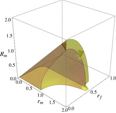
(a) $N_{H}=1$.

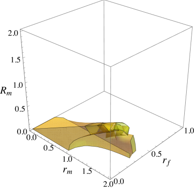
(b) $N_{H}=2$.

Figure 2: The allowed parameters ($r_{m}$, $r_{f}$, and $R_{m}$) regions for level crossing. The left and right panels correspond to $N_{H}=1$ and 2, respectively. Note that here we just show the regions with $0<r_{m}<2$, $0<r_{f}<1$, and $0<R_{m}<2$.

Let us discuss the temperature-dependent behaviors of the axions when the mass mixing occurs in figure 3. At high temperatures, the light axion eigenstate $a_{2}$ comprises the QCD axion, while the heavy axion eigenstate $a_{1}$ comprises the ALP. With the cosmic temperature decreasing, the level crossing would take place, the masse eigenvalues $m_{1}(T)$ and $m_{2}(T)$ would approach to each other at $T_{\times}$ and then move away from each other. After that, the $a_{2}$ comprises the ALP, and the $a_{1}$ comprises the QCD axion. The level crossing can lead to the adiabatic energy density transition between the two axion eigenstates Ho:2018qur , or between the QCD axion and ALP, which will be discussed next. Since $r_{m}$ determines the ALP mass $m_{A}$, it will mainly affect the temperature $T_{\times}$. For different values of $N_{H}$, we find that the values of $m_{2}(T)$ are different at high temperatures, while the values of $m_{1}(T)$ are almost coincident from high to low temperatures. For different values of $r_{f}$, the main difference is their behaviors at $T_{\times}$, which maybe the effect of avoided level crossing for larger $r_{f}$ as discussed in ref. Cyncynates:2023esj , but we will not discuss it more in this context. In order for the level crossing to occur, we note that there is a relation that should be satisfied, the value of $m_{2}(T)$ at high temperatures should not be larger than the ALP mass, $\rm i.e.$, $r_{m}>N_{H}R_{m}$. There is no level crossing in the case $r_{m}\leq N_{H}R_{m}$, which can be seen from figure 3. However, we find this is already given in eq. (40) with $r_{m}^{2}-N_{H}^{2}R_{m}^{2}>\left(1+N_{H}\right)^{2}r_{m}^{2}r_{f}^{2}>0$. Therefore, the allowed regions in figure 2 are still valid for level crossing.

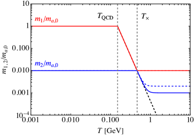
(a) $r_{m}=0.01$, $r_{f}=0.01$, $R_{m}=0.001$.

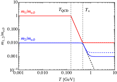
(b) $r_{m}=0.01$, $r_{f}=0.1$, $R_{m}=0.001$.

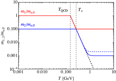
(c) $r_{m}=0.1$, $r_{f}=0.01$, $R_{m}=0.001$.

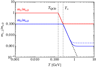
(d) $r_{m}=0.1$, $r_{f}=0.1$, $R_{m}=0.001$.

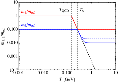
(e) $r_{m}=0.1$, $r_{f}=0.01$, $R_{m}=0.01$.

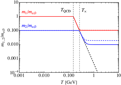
(f) $r_{m}=0.1$, $r_{f}=0.1$, $R_{m}=0.01$.

Figure 3: The normalized mass eigenvalues $m_{1,2}(T)/m_{a,0}$ as functions of the cosmic temperature $T$ with several typical parameter sets for level crossing. The red and blue solid (dashed) lines correspond to the mass eigenvalues $m_{1}(T)$ and $m_{2}(T)$ with $N_{H}=1$ ($N_{H}=2$), respectively. The black dashed line corresponds to the QCD axion mass $m_{a}(T)$. The two vertical gray lines represent the temperatures $T_{\rm QCD}$ and $T_{\times}$, respectively. Here we set $f_{a}=10^{12}\,\rm GeV$.

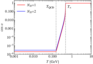
(a) $r_{m}=0.01$, $r_{f}=0.01$, $R_{m}=0.001$.

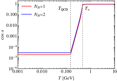
(b) $r_{m}=0.01$, $r_{f}=0.1$, $R_{m}=0.001$.

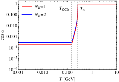
(c) $r_{m}=0.1$, $r_{f}=0.01$, $R_{m}=0.001$.

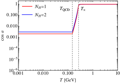
(d) $r_{m}=0.1$, $r_{f}=0.1$, $R_{m}=0.001$.

(e) $r_{m}=0.1$, $r_{f}=0.01$, $R_{m}=0.01$.

(f) $r_{m}=0.1$, $r_{f}=0.1$, $R_{m}=0.01$.

Figure 4: The mass mixing angle $\cos\alpha$ as functions of $T$ with the parameter sets in figure 3. The red and blue lines correspond to the cases $N_{H}=1$ and 2, respectively. The two vertical gray lines represent the temperatures $T_{\rm QCD}$ and $T_{\times}$, respectively. Note that the behaviors of the mixing angle in panels (e) and (f) almost coincide with that in (c) and (d), respectively.

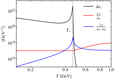
(a) $r_{m}=0.01$, $r_{f}=0.01$, $R_{m}=0.001$.

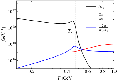
(b) $r_{m}=0.01$, $r_{f}=0.1$, $R_{m}=0.001$.

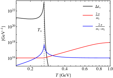
(c) $r_{m}=0.1$, $r_{f}=0.01$, $R_{m}=0.001$.

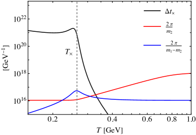
(d) $r_{m}=0.1$, $r_{f}=0.1$, $R_{m}=0.001$.

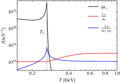
(e) $r_{m}=0.1$, $r_{f}=0.01$, $R_{m}=0.01$.

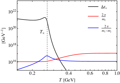
(f) $r_{m}=0.1$, $r_{f}=0.1$, $R_{m}=0.01$.

Figure 5: The three terms in eq. (43) as functions of $T$ with the parameter sets in figure 3. The black, red, and blue lines represent the values of $\Delta t_{\times}$, $2\pi/m_{2}(T)$, and $2\pi/\left(m_{1}(T)-m_{2}(T)\right)$, respectively. The vertical gray lines represent the temperature $T_{\times}$. Note that we just show the case $N_{H}=1$.

In addition, we also show the mass mixing angle $\cos\alpha$ as functions of the cosmic temperature in figure 4, in which the parameter sets correspond to figure 3. The red and blue lines correspond to the cases $N_{H}=1$ and 2, respectively. At high temperatures, we have the constant values of $\cos\alpha=1$ ($\alpha=0$) until the level crossing occurs at $T_{\times}$. Then the mass mixing angle drops rapidly and stabilizes at a small value, which lasts for a very short time, $\Delta t_{\times}$. We find that the behaviors of the mixing angle in panels (e) and (f) almost coincide with that in (c) and (d), respectively. This is because that, compared with the parameters $r_{m}$ and $r_{f}$, the $R_{m}$ has a little contribution to the temperature $T_{\times}$ and the mixing angle $\cos\alpha$. However, $R_{m}$ is important to determine the final axion DM abundance, which can be seen in next subsection. Note that the behaviors of the mass mixing angle are not always same as shown in figure 4, which are exactly the cases for level crossing in our scenario. In fact, the alteration in the mixing angle is not significant or even unchanged if there is no level crossing in the mixing, which is not the interest of this context and we do not show it.

Then we briefly discuss the adiabatic energy density transition between the two axion eigenstates in this scenario, it is necessary to determine the axion energy density. In the mass mixing, the adiabatic transition will take place if both the comoving axion numbers of the eigenstates $a_{1}$ and $a_{2}$ are separately conserved at the level crossing devaud:hal-00197565 , which lasts for a parametric duration

$$\Delta T_{\times}=\bigg{|}\frac{1}{\cos\alpha(T)}\frac{{\rm d}\cos\alpha(T)}{{\rm d}T}\bigg{|}^{-1}_{T=T_{\times}}\,,$$ (42)

corresponding to the time $\Delta t_{\times}$. The condition for adiabatic transition reads Ho:2018qur

$$\Delta t_{\times}\gg\max\left[\frac{2\pi}{m_{2}(T)}\bigg{|}_{T=T_{\times}},\,\frac{2\pi}{m_{1}(T)-m_{2}(T)}\bigg{|}_{T=T_{\times}}\right]\,,$$ (43)

which has a complicated analytical form, and we just check it numerically. We show the values of the three terms in eq. (43) in figure 5. The parameter sets correspond to figure 3 with $N_{H}=1$. The black, red, and blue lines represent the values of $\Delta t_{\times}$, $2\pi/m_{2}(T)$, and $2\pi/\left(m_{1}(T)-m_{2}(T)\right)$, respectively. In these plots, we find that eq. (43) can be satisfied at $T_{\times}$. Note that we do not show the case $N_{H}=2$, which has a similar distribution with $N_{H}=1$.

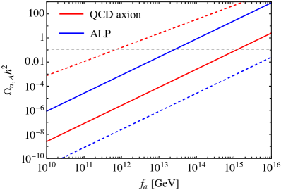
(a) $r_{m}=0.01$, $r_{f}=0.01$, $R_{m}=0.001$.

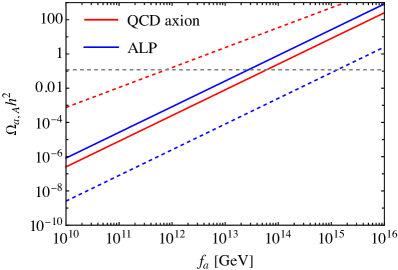
(b) $r_{m}=0.01$, $r_{f}=0.1$, $R_{m}=0.001$.

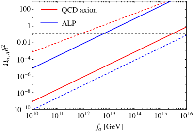
(c) $r_{m}=0.1$, $r_{f}=0.01$, $R_{m}=0.001$.

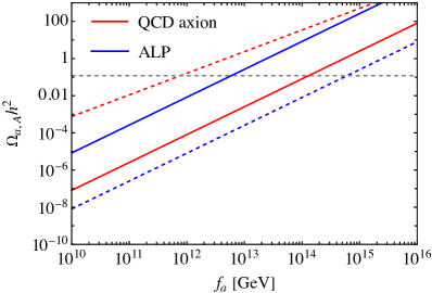
(d) $r_{m}=0.1$, $r_{f}=0.1$, $R_{m}=0.001$.

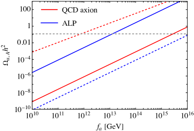
(e) $r_{m}=0.1$, $r_{f}=0.01$, $R_{m}=0.01$.

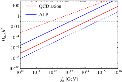
(f) $r_{m}=0.1$, $r_{f}=0.1$, $R_{m}=0.01$.

Figure 6: The axion DM abundances as functions of the QCD axion decay constant $f_{a}$ with the parameter sets in figure 3. The red and blue solid (dashed) lines represent the QCD axion and ALP abundances with (without) the mixing, respectively. The horizontal gray line represents the observed cold DM abundance, $\Omega_{\rm DM}h^{2}\simeq 0.12$. Here we just show the case $N_{H}=1$.

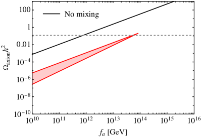
(a) $r_{m}=0.01$, $r_{f}=0.01$, $N_{H}=1$.

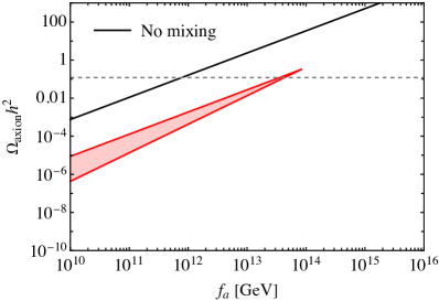
(b) $r_{m}=0.01$, $r_{f}=0.01$, $N_{H}=2$.

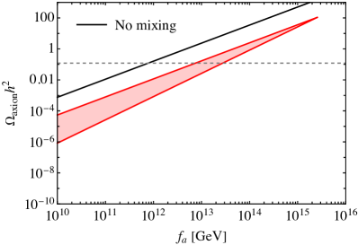
(c) $r_{m}=0.1$, $r_{f}=0.01$, $N_{H}=1$.

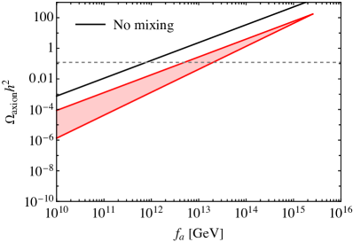
(d) $r_{m}=0.1$, $r_{f}=0.01$, $N_{H}=2$.

Figure 7: The total axion DM abundances as functions of $f_{a}$. The black solid lines represent the total axion DM abundance without the mixing. The red triangular areas represent the total axion DM abundances in the mixing set with the limits of $R_{m}$. The horizontal gray line represents the observed cold DM abundance.

3.3 Axion dark matter abundance

In this subsection, we investigate the axion DM abundance in our scenario. In this case, the ratios of the axion number density of the QCD axion and ALP to the entropy density at the corresponding oscillation temperatures are given by

$$\frac{n_{a}(T)}{s(T)}\bigg{|}_{T=T_{{\rm osc},A}}\simeq\frac{1}{2}\frac{m_{A}}{s(T_{{\rm osc},A})}f_{A}^{2}\left\langle\theta_{i,A}^{2}f(\theta_{i})\right\rangle\,,$$ (44)

and

$$\frac{n_{A}(T)}{s(T)}\bigg{|}_{T=T^{\prime}_{{\rm osc},a}}\simeq\frac{1}{2}\frac{N_{H}m_{\cancel{\rm PQ}}}{s(T^{\prime}_{{\rm osc},a})}f_{a}^{2}\left\langle\theta_{i}^{2}f^{\prime}(\theta_{i})\right\rangle\,,$$ (45)

where we set the initial misalignment angles $\theta_{i}=1$ and $\theta_{i,A}=1$. The QCD axion and ALP DM abundance at present are given by

$$\Omega_{a}h^{2}=m_{a,0}\frac{n_{a}(T)}{s(T)}\bigg{|}_{T=T_{{\rm osc},A}}\frac{s(T_{0})}{\rho_{\rm crit}h^{-2}}\,,$$ (46)

and

$$\Omega_{A}h^{2}=m_{A}\frac{n_{A}(T)}{s(T)}\bigg{|}_{T=T^{\prime}_{{\rm osc},a}}\frac{s(T_{0})}{\rho_{\rm crit}h^{-2}}\,.$$ (47)

We show the axion DM abundances as functions of the QCD axion decay constant $f_{a}$ in figure 6 with the parameter sets in figure 3. The red and blue solid lines represent the QCD axion and ALP abundances with the mixing in this work, respectively. While the corresponding dashed lines represent the abundances without the mixing, see eqs. (8) and (11). The horizontal gray line represents the observed cold DM abundance, $\Omega_{\rm DM}h^{2}\simeq 0.12$, which suggests an initial misalignment angle $\theta_{i}\sim\mathcal{O}(1)$ for the no-mixing QCD axion DM with $f_{a}=10^{12}\,\rm GeV$. For these parameter sets, we find that the QCD axion is dominated the axion abundance if there is no mixing (dashed lines), while the ALP is dominated in the mixing (solid lines). Since the parameter $N_{H}$ only has a little contribution to the mixing ALP abundance (the blue solid line), and the case $N_{H}=2$ almost coincide with $N_{H}=1$, we just show the case $N_{H}=1$ in these plots. However, $N_{H}$ has a contribution to determine the lower limit of $R_{m}$ [eq. 18], which will be discussed next.

Finally, we discuss the total axion DM abundance at present in this scenario, which is composed of the QCD axion and ALP DM abundances

$$\begin{aligned} \Omega_{\rm axion}h^{2}&=\Omega_{a}h^{2}+\Omega_{A}h^{2}\\ &=\left(m_{a,0}\frac{n_{a}(T)}{s(T)}\bigg{|}_{T=T_{{\rm osc},A}}+m_{A}\frac{n_{A}(T)}{s(T)}\bigg{|}_{T=T^{\prime}_{{\rm osc},a}}\right)\frac{s(T_{0})}{\rho_{\rm crit}h^{-2}}\,.\end{aligned}$$ (48)

We show the total axion DM abundance in figure 7. The black solid lines represent the total axion DM abundance without the mixing. Since the QCD axion is dominated in the no-mixing, the total axion DM abundance is mainly related to $f_{a}$ and $\theta_{i}$. Here we also set the initial misalignment angles $\theta_{i}=1$ and $\theta_{i,A}=1$. The red triangular areas represent the total axion DM abundances in the mixing set with the limits of $R_{m}$, the upper limit $R_{m}<r_{m}/N_{H}$ and the lower limit in eq. (18). Since the ALP is dominated in the mixing, the total axion DM abundance is mainly related to $r_{m}$, $R_{m}$, $N_{H}$, $f_{a}$, and $\theta_{i}$, but not to $r_{f}$ and $\theta_{i,A}$, we just show a typical value of $r_{f}=0.01$. Compared with the conventional case, the total axion DM abundance is significantly suppressed.

4 Conclusion

In this paper, we have investigated the axion mass mixing between the QCD axions and ALPs in the axiverse with the explicit PQ symmetry breaking in the early Universe. We first review the QCD axion and ALP DM with the misalignment mechanism, and introduce the mass mixing between them. Then we study this mass mixing with an explicit PQ symmetry breaking term. Exactly, we consider the mass mixing with one QCD axion and one ALP in this work.

We study the dynamics of the axions and their cosmological evolutions in detail when the level crossing occurs in this scenario. The allowed parameters ($r_{m}$, $r_{f}$, and $R_{m}$) regions of the condition for level crossing are shown. Since we consider a case that the QCD axion starts to oscillate due to the explicit PQ symmetry breaking term before the conventional case, the parameter $R_{m}$ has a lower limit. On the other hand, in order for the level crossing to take place in the mixing, there is a relation between $m_{\cancel{\rm PQ}}$ and $m_{A}$ that should be satisfied, which indicates that $R_{m}$ has an upper limit. Then we show the evolutions of the normalized mass eigenvalues and the mass mixing angle with several typical parameter sets for level crossing. We also check the condition for adiabatic transition with these parameter sets, which is necessary to determine the axion energy density. Finally, we focus our attention on the axion DM abundance and show the abundance distributions of the QCD axion and ALP DM. Also with above parameter sets, if there is no mass mixing between the QCD axion and ALP, the total axion DM abundance is dominated by the QCD axion. While with the mixing in our scenario, the ALP dominates the axion DM abundance. Using the limits of $R_{m}$, we also show the distributions of the total axion abundance. We find that, in the presence of the explicit PQ symmetry breaking term in the mixing, the total axion DM abundance is significantly suppressed.

References

- (1) R. Peccei and H. R. Quinn, Constraints Imposed by CP Conservation in the Presence of Instantons, Phys. Rev. D 16 (1977) 1791–1797.
- (2) R. Peccei and H. R. Quinn, CP Conservation in the Presence of Instantons, Phys. Rev. Lett. 38 (1977) 1440–1443.
- (3) S. Weinberg, A New Light Boson?, Phys. Rev. Lett. 40 (1978) 223–226.
- (4) F. Wilczek, Problem of Strong and Invariance in the Presence of Instantons, Phys. Rev. Lett. 40 (1978) 279–282.
- (5) J. E. Kim, Weak Interaction Singlet and Strong CP Invariance, Phys. Rev. Lett. 43 (1979) 103.
- (6) M. A. Shifman, A. I. Vainshtein and V. I. Zakharov, Can Confinement Ensure Natural CP Invariance of Strong Interactions?, Nucl. Phys. B 166 (1980) 493–506.
- (7) M. Dine, W. Fischler and M. Srednicki, A Simple Solution to the Strong CP Problem with a Harmless Axion, Phys. Lett. B 104 (1981) 199–202.
- (8) A. R. Zhitnitsky, On Possible Suppression of the Axion Hadron Interactions. (In Russian), Sov. J. Nucl. Phys. 31 (1980) 260.
- (9) G. ’t Hooft, Symmetry Breaking Through Bell-Jackiw Anomalies, Phys. Rev. Lett. 37 (1976) 8–11.
- (10) G. ’t Hooft, Computation of the Quantum Effects Due to a Four-Dimensional Pseudoparticle, Phys. Rev. D 14 (1976) 3432–3450. [Erratum: Phys.Rev.D 18, 2199 (1978)].
- (11) J. Preskill, M. B. Wise and F. Wilczek, Cosmology of the Invisible Axion, Phys. Lett. B 120 (1983) 127–132.
- (12) L. Abbott and P. Sikivie, A Cosmological Bound on the Invisible Axion, Phys. Lett. B 120 (1983) 133–136.
- (13) M. Dine and W. Fischler, The Not So Harmless Axion, Phys. Lett. B 120 (1983) 137–141.
- (14) R. Mayle, J. R. Wilson, J. R. Ellis, K. A. Olive, D. N. Schramm and G. Steigman, Constraints on Axions from SN 1987a, Phys. Lett. B 203 (1988) 188–196.
- (15) G. Raffelt and D. Seckel, Bounds on Exotic Particle Interactions from SN 1987a, Phys. Rev. Lett. 60 (1988) 1793.
- (16) M. S. Turner, Axions from SN 1987a, Phys. Rev. Lett. 60 (1988) 1797.
- (17) L. B. Leinson, Axion mass limit from observations of the neutron star in Cassiopeia A, JCAP 08 (2014) 031, [1405.6873].
- (18) K. Hamaguchi, N. Nagata, K. Yanagi and J. Zheng, Limit on the Axion Decay Constant from the Cooling Neutron Star in Cassiopeia A, Phys. Rev. D 98 (2018) 103015, [1806.07151].
- (19) M. Buschmann, C. Dessert, J. W. Foster, A. J. Long and B. R. Safdi, Upper Limit on the QCD Axion Mass from Isolated Neutron Star Cooling, Phys. Rev. Lett. 128 (2022) 091102, [2111.09892].
- (20) L. M. Carpenter, M. Dine and G. Festuccia, Dynamics of the Peccei Quinn Scale, Phys. Rev. D 80 (2009) 125017, [0906.1273].
- (21) W. Yin, Scale and quality of Peccei-Quinn symmetry and weak gravity conjectures, JHEP 10 (2020) 032, [2007.13320].
- (22) M. Kamionkowski and J. March-Russell, Planck scale physics and the Peccei-Quinn mechanism, Phys. Lett. B 282 (1992) 137–141, [hep-th/9202003].
- (23) S. M. Barr and D. Seckel, Planck scale corrections to axion models, Phys. Rev. D 46 (1992) 539–549.
- (24) S. Ghigna, M. Lusignoli and M. Roncadelli, Instability of the invisible axion, Phys. Lett. B 283 (1992) 278–281.
- (25) R. Kallosh, A. D. Linde, D. A. Linde and L. Susskind, Gravity and global symmetries, Phys. Rev. D 52 (1995) 912–935, [hep-th/9502069].
- (26) T. Banks and N. Seiberg, Symmetries and Strings in Field Theory and Gravity, Phys. Rev. D 83 (2011) 084019, [1011.5120].
- (27) D. Harlow and H. Ooguri, Symmetries in quantum field theory and quantum gravity, Commun. Math. Phys. 383 (2021) 1669–1804, [1810.05338].
- (28) M. Reece, TASI Lectures: (No) Global Symmetries to Axion Physics, 2304.08512.
- (29) T. Higaki, K. S. Jeong, N. Kitajima and F. Takahashi, Quality of the Peccei-Quinn symmetry in the Aligned QCD Axion and Cosmological Implications, JHEP 06 (2016) 150, [1603.02090].
- (30) K. S. Jeong, K. Matsukawa, S. Nakagawa and F. Takahashi, Cosmological effects of Peccei-Quinn symmetry breaking on QCD axion dark matter, JCAP 03 (2022) 026, [2201.00681].
- (31) K. Choi, H. Kim and S. Yun, Natural inflation with multiple sub-Planckian axions, Phys. Rev. D 90 (2014) 023545, [1404.6209].
- (32) T. Higaki and F. Takahashi, Natural and Multi-Natural Inflation in Axion Landscape, JHEP 07 (2014) 074, [1404.6923].
- (33) T. Higaki and F. Takahashi, Axion Landscape and Natural Inflation, Phys. Lett. B 744 (2015) 153–159, [1409.8409].
- (34) K. Choi and S. H. Im, Realizing the relaxion from multiple axions and its UV completion with high scale supersymmetry, JHEP 01 (2016) 149, [1511.00132].
- (35) D. E. Kaplan and R. Rattazzi, Large field excursions and approximate discrete symmetries from a clockwork axion, Phys. Rev. D 93 (2016) 085007, [1511.01827].
- (36) A. J. Long, Cosmological Aspects of the Clockwork Axion, JHEP 07 (2018) 066, [1803.07086].
- (37) T. Higaki, K. S. Jeong, N. Kitajima and F. Takahashi, The QCD Axion from Aligned Axions and Diphoton Excess, Phys. Lett. B 755 (2016) 13–16, [1512.05295].
- (38) S. Nakagawa, F. Takahashi and M. Yamada, Trapping Effect for QCD Axion Dark Matter, JCAP 05 (2021) 062, [2012.13592].
- (39) N. Kitajima and F. Takahashi, Primordial Black Holes from QCD Axion Bubbles, JCAP 11 (2020) 060, [2006.13137].
- (40) H.-J. Li, QCD axion bubbles from the hidden SU(N) gauge symmetry breaking, 2303.04537.
- (41) H.-J. Li, Y.-Q. Peng, W. Chao and Y.-F. Zhou, Can supermassive black holes triggered by general QCD axion bubbles?, 2304.00939.
- (42) K. Kasai, M. Kawasaki, N. Kitajima, K. Murai, S. Neda and F. Takahashi, Clustering of Primordial Black Holes from QCD Axion Bubbles, 2305.13023.
- (43) M. B. Green and J. H. Schwarz, Anomaly Cancellation in Supersymmetric D=10 Gauge Theory and Superstring Theory, Phys. Lett. B 149 (1984) 117–122.
- (44) E. Witten, Some Properties of O(32) Superstrings, Phys. Lett. B 149 (1984) 351–356.
- (45) J. Halverson, C. Long, B. Nelson and G. Salinas, Towards string theory expectations for photon couplings to axionlike particles, Phys. Rev. D 100 (2019) 106010, [1909.05257].
- (46) H.-J. Li, J.-G. Guo, X.-J. Bi, S.-J. Lin and P.-F. Yin, Limits on axion-like particles from Mrk 421 with 4.5-year period observations by ARGO-YBJ and Fermi-LAT, Phys. Rev. D 103 (2021) 083003, [2008.09464].
- (47) D. Cyncynates, T. Giurgica-Tiron, O. Simon and J. O. Thompson, Resonant nonlinear pairs in the axiverse and their late-time direct and astrophysical signatures, Phys. Rev. D 105 (2022) 055005, [2109.09755].
- (48) H.-J. Li, Probing photon-ALP oscillations from the flat spectrum radio quasar 4C+21.35, Phys. Lett. B 829 (2022) 137047, [2203.08573].
- (49) H.-J. Li and W. Chao, Axion effects on gamma-ray spectral irregularities with AGN redshift uncertainty, Phys. Rev. D 107 (2023) 063031, [2211.00524].
- (50) D. Cadamuro and J. Redondo, Cosmological bounds on pseudo Nambu-Goldstone bosons, JCAP 02 (2012) 032, [1110.2895].
- (51) P. Arias, D. Cadamuro, M. Goodsell, J. Jaeckel, J. Redondo and A. Ringwald, WISPy Cold Dark Matter, JCAP 06 (2012) 013, [1201.5902].
- (52) W. Chao, M. Jin, H.-J. Li and Y.-Q. Peng, Axion-like Dark Matter from the Type-II Seesaw Mechanism, 2210.13233.
- (53) P. Svrcek and E. Witten, Axions In String Theory, JHEP 06 (2006) 051, [hep-th/0605206].
- (54) A. Arvanitaki, S. Dimopoulos, S. Dubovsky, N. Kaloper and J. March-Russell, String Axiverse, Phys. Rev. D 81 (2010) 123530, [0905.4720].
- (55) M. Demirtas, N. Gendler, C. Long, L. McAllister and J. Moritz, PQ axiverse, JHEP 06 (2023) 092, [2112.04503].
- (56) C. T. Hill and G. G. Ross, Models and New Phenomenological Implications of a Class of Pseudogoldstone Bosons, Nucl. Phys. B 311 (1988) 253–297.
- (57) N. Kitajima and F. Takahashi, Resonant conversions of QCD axions into hidden axions and suppressed isocurvature perturbations, JCAP 01 (2015) 032, [1411.2011].
- (58) R. Daido, N. Kitajima and F. Takahashi, Level crossing between the QCD axion and an axionlike particle, Phys. Rev. D 93 (2016) 075027, [1510.06675].
- (59) S.-Y. Ho, K. Saikawa and F. Takahashi, Enhanced photon coupling of ALP dark matter adiabatically converted from the QCD axion, JCAP 10 (2018) 042, [1806.09551].
- (60) R. Daido, N. Kitajima and F. Takahashi, Domain Wall Formation from Level Crossing in the Axiverse, Phys. Rev. D 92 (2015) 063512, [1505.07670].
- (61) K. Murai, F. Takahashi and W. Yin, The QCD Axion: A Unique Player in the Axiverse with Mixings, 2305.18677.
- (62) D. Cyncynates and J. O. Thompson, Heavy QCD axion dark matter from avoided level crossing, 2306.04678.
- (63) L. Wolfenstein, Neutrino Oscillations in Matter, Phys. Rev. D 17 (1978) 2369–2374.
- (64) S. P. Mikheyev and A. Y. Smirnov, Resonance Amplification of Oscillations in Matter and Spectroscopy of Solar Neutrinos, Sov. J. Nucl. Phys. 42 (1985) 913–917.
- (65) S. P. Mikheev and A. Y. Smirnov, Resonant amplification of neutrino oscillations in matter and solar neutrino spectroscopy, Nuovo Cim. C 9 (1986) 17–26.
- (66) S. Borsanyi et al., Calculation of the axion mass based on high-temperature lattice quantum chromodynamics, Nature 539 (2016) 69–71, [1606.07494].
- (67) G. Grilli di Cortona, E. Hardy, J. Pardo Vega and G. Villadoro, The QCD axion, precisely, JHEP 01 (2016) 034, [1511.02867].
- (68) D. H. Lyth, Axions and inflation: Sitting in the vacuum, Phys. Rev. D 45 (1992) 3394–3404.
- (69) L. Visinelli and P. Gondolo, Dark Matter Axions Revisited, Phys. Rev. D 80 (2009) 035024, [0903.4377].
- (70) M. S. Turner, Cosmic and Local Mass Density of Invisible Axions, Phys. Rev. D 33 (1986) 889–896.
- (71) Planck collaboration, N. Aghanim et al., Planck 2018 results. VI. Cosmological parameters, Astron. Astrophys. 641 (2020) A6, [1807.06209]. [Erratum: Astron.Astrophys. 652, C4 (2021)].
- (72) M. Devaud, V. Leroy, J.-C. Bacri and T. Hocquet, “The adiabatic invariant of any harmonic oscillator : an unexpected application of Glauber’s formalism.” working paper or preprint, Dec., 2007.