Application of BERT in Wind Power Forecasting-Teletraan’s Solution in Baidu KDD Cup 2022

Abstract.

Nowadays, wind energy has drawn increasing attention as its important role in carbon neutrality and sustainable development. When wind power is integrated into the power grid, precise forecasting is necessary for the sustainability and security of the system. However, the unpredictable nature and long sequence prediction make it especially challenging. In this technical report, we introduce the BERT model applied for Baidu KDD Cup 2022, and the daily fluctuation is added by post-processing to make the predicted results in line with daily periodicity. Our solution achieves 3rd place of 2490 teams. The code is released at github.com/LongxingTan/KDD2022-Baidu

1. Introduction

Wind energy plays an important role in carbon neutrality. The precise prediction of wind power can help its integration into the power system with sustainability and security of supply (Hanifi et al., 2020). However, the unpredictable nature of wind makes it challenging, especially for long sequence forecasting.

Transformer models are proposed for long sequence forecasting in recent research (Wen et al., 2022). To utilize the advantage of its capturing long dependencies, we implement a BERT model for wind power future prediction. Our solution is a single model with a single BERT block, with both accuracy and efficiency.

1.1. Dataset

A unique spatial, dynamic wind power forecasting dataset-SDWPF (Zhou et al., 2022) is provided by Baidu and Longyuan for this competition. The training data consists of 245-day records for 134 turbines. Its interval is 10 minutes. Additionally, each sample has wind speed, wind direction, relative power, the temperature, in total ten parameters. The procedures of data preprocessing are introduced in Section 4.1.

1.2. Task

Given at most 14-day historical data, participants need to predict the future 2 days’ wind power for every turbine and every 10 minutes. There are 142 samples provided in the last phase to evaluate the model performance, and each sample is randomly sampled over several months. Inference on the test data needs to be finished in 10 hours in the online environment.

1.3. Evaluation

The performance is measured by the average of RMSE (root mean square error) and MAE (mean absolute error) for each turbine as metrics score. There are some invalid values in ground truth labels such as zero values, missing values, and unknown values. Based on the task description, the metrics score for those invalid values in ground truth is set to zero to ignore them.

2. Related Work

There is already a long history of wind power forecasting. The mainstream approaches include the physical approach, statistical approach and the ensemble approach (Kariniotakis et al., 2004). The physical approach uses the meteorological service and numerical weather prediction to predict the future in a short.

The statistical approach builds a model using statistical methods. The commonly used time series prediction methods include ARIMA, statistical models(Cao and Gui, 2018), and deep learning methods (Swaminathan et al., 2021). Besides, now the long sequence time series forecasting also catches lots of attention from the real-world requirements. Recently, the prediction capacity is increased by the latest transformer family, such as the Informer (Zhou et al., 2021) and Autoformer (Wu et al., 2021) model. Informer uses the sparse attention and one-time decoder to accelerate the inference. The Autoformer uses a decomposition method and frequency domain attention to improve its capacity in long sequence prediction. The spatial-temporal approach is also a promising way for wind power forecasting (Li and Armandpour, 2022). The spatial information can be used to improve the forecasting accuracy (Fang et al., 2020). So batches of new models are proposed and achieve good results with the development of graph neural networks, like GCN-LSTM, Graph Wavenet (Yu et al., 2017), Graph Convolutional Network (Stańczyk and Mehrkanoon, 2021) and Graph Attention Network (Zhou et al., 2020).

3. Solution Overview

In this section, we explain the main components of our solution. The overall architecture of our method is shown in Figure 1.

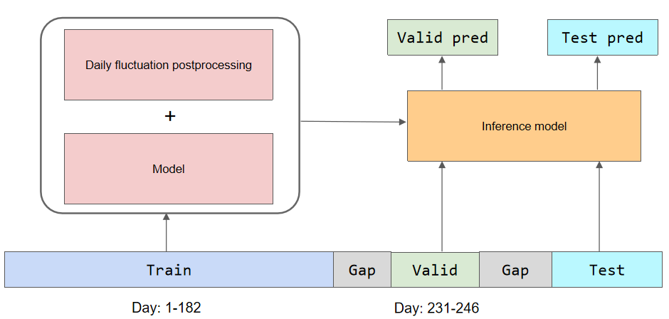
Figure 1. Solution architecture

Solution architecture

We implement two pipelines to treat the problem either as a multi-step time series prediction or a spatial-temporal prediction. What’s more, we can choose to predict the generated wind power directly or to predict the wind speed first and then transfer it into wind power(Wang et al., 2021b). Besides we tried training different time scale models to handle the long sequence prediction.

When it comes to a time series task, each turbine can generate its samples independently. Because the whole wind farm has a very similar trend, the time series model can capture the long-term seasonality better for long sequence prediction. We tried KNN, LightGBM, RNN, TCN, BERT, Seq2seq, Wavenet, and Transformer models.

When it comes to a spatial-temporal task, the promising models are like GCN-LSTM, ConvLSTM (Shi et al., 2015), GraphWavenet (Wu et al., 2019), Graph Transformer (Yun et al., 2019) and spatial CNN models. If spatial information and spatial distribution could be captured, it’s assumed to be helpful for future prediction as well (Wang et al., 2021a).

4. Detailed method

4.1. Data preprocessing

We create the samples for each turbine every 10 minutes by sliding the window to get more training data. There are NANs and invalid values in the data. We use the corresponding previous value to fill them for training and inference. And we use a min-max scaler to standardize the features into scope between zero and one, but leave the target column alone.

4.2. Features

To avoid over-fitting, we try to use as fewer features as possible. The commonly used lag features, rolling features, and time features are not helpful according to our experiments. The temperature is noisy, so the temperature feature is not involved.

Given the unpredictable nature, it’s hard to predict the future trend and seasonality perfectly. So we try to add spatial information and temporal information as features to improve the prediction performance. But they are not helpful in our experiments. So finally we only choose the wind speed and wind direction to train the model.

4.3. Models

We choose a single BERT model (Devlin et al., 2018) as our final model to handle the long dependencies for long sequence prediction. The BERT model has been widely used in all tasks in natural language processing since its publication. In computer vision, speech, and time series, it has also been widely investigated and it achieves fruitful results since then. The detailed model structure we use is shown in Figure 2.

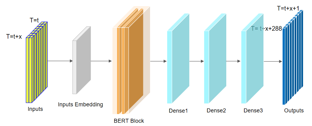
Figure 2. BERT model structure

BERT model structure

A token embedding layer without positional encoding can project the raw feature space into the attention space. The experiments show there is not a significant influence having positional encoding or not. The module following the embedding layer is a standard BERT encoder, with self-attention layer, feed-forward network, layer normalization and residual connection. Then 3 dense layers with dropout can capture the crossed information from time and features. The hidden sizes of the last dense layer are equal to the predicted steps 288. And our experiments show that layer normalization and residual connection are both important that can’t be ignored. The detailed model configuration is shown in Table 1.

Table 1. BERT model configuration

Hyper-parameters	Value
Train sequence lengths	288
Predict sequence lengths	288
Number of encoder layers	1
Attention hidden sizes	32
Number of attention heads	1
Attention drop out rate	0
Feed forward layer hidden sizes	32
Feed forward layer dropout rate	0
Dense1 hidden sizes	512
Dense1 dropout rate	0.25
Dense2 hidden sizes	1024
Dense2 dropout rate	0.25
Dense3 hidden sizes	288

4.4. Training

We use a GTX 1080Ti for training our models, and the BERT model costs about 90 minutes. An RMSE loss function and Adam optimizer are used for training as shown in Table 2.

Table 2. Training configuration

Training parameters	Value
Batch sizes	1024
Training epochs	3
Learning rate	0.005
Optimizer	Adam

4.5. Post-processing

A series of post-processing strategies are employed to further improve forecasting accuracy. We know it’s important for better prediction to capture the trend, seasonality, and spatial information. However, we find our forecasting results don’t have obvious daily periodicity, while the descriptive analysis in historical data shows it’s strong for most days. So we propose two ways to solve it. The first one is to add the daily fluctuation by post-processing. The daily average fluctuation is calculated and added to the prediction result directly. The second way is to optimize the model to make the model learn the daily fluctuation by itself, in which the time or wind information information is added as the decoder feature to decode the BERT output further. In the end, the latter methods in models are not as good as the first way in our experiments.

To give more details, we calculate the average wind power for every interval. Then the daily sequence is standardized to zero and one. Because the wind power is between 0 and 1620, a multiplier of 36 is chosen to magnify it according to local validation and the leaderboard. The multiplier could force the daily fluctuation to influence the predictions in a reasonable scope. For larger values, we further magnify them by multiplying a constant value like 1.1. Finally, the daily fluctuation sequence needs to match the predicted start time by shifting it, as not all predictions start from 00:00. In this way, the predicted future sequence could reflect the daily period with the same daily fluctuation level with historical data.

5. Experiment

5.1. Validation strategy

There are 3 phases of online test data in the competition, with a temporal relationship. So we leave a gap between offline training data and validation data to simulate this scenario. The training data we choose is between the 1st and 181st day, and the offline validation data is between the 231st and 245th day as shown in Figure1.

Considering we use 250982 valid samples as local validation, while the online test data use only 150-200 samples, we submit the model unless the local validation score is improved to decrease the risk of shaking down. Because the concept drift issue occurs for time-related task, in the last phase, we modified the model based on our best model in the second phase.

5.2. Results and comparison

In this section, we compare the different models’ performances from our experiments. The results of the time series model and spatial-temporal model are shown in Table 3. To make the local validation comparable with the leaderboard, the MAE, RMSE and metrics scores are transferred to the sum of 195 samples’ results.

Table 3. Performance comparison of models

Model	Local MAE	Local RMSE	Local score	Leaderboard score (phase II)
BERT	299	365	58.1	44.6
LSTM	305	369	58.9	44.8
TCN	310	371	59.4	45.1
KNN	316	368	60.6	unsubmit
LGB	319	386	61.4	unsubmit
Transformer	311	374	60.0	48.5
Seq2seq	296	366	57.6	47.1
Wavenet	306	370	59.1	47.9
GCN-LSTM	228	362	54.5	48.2

We can see that the deep learning methods behave better than statistical learning methods like KNN or LGB in our experiments. The wind power data is homogeneous, without important categorical information or crossed information, so the deep learning model can handle this task very well. The spatial information definitely could help more accurate predictions. As for the spatial relationship, we tried the spatial-temporal models to capture the spatial relationship automatically, but our implementations are not so successful in the leaderboard. Now that every turbine’s power trend is quite similar, we focus more on its temporal properties afterward.

6. Conclusion and future work

In this technical report, we introduce our BERT solution for Baidu KDD Cup 2022 wind power forecasting. The BERT model can predict the primary trend for the long sequence prediction, and the daily fluctuation is added by post-processing to make the prediction with daily periodicity. Though the single BERT model is accurate and efficient, it can still be enhanced in many ways like transfer learning or the graph model.

- (1)
- Cao and Gui (2018) Yukun Cao and Liai Gui. 2018. Multi-step wind power forecasting model using LSTM networks, similar time series and LightGBM. In 2018 5th International Conference on Systems and Informatics (ICSAI). IEEE, 192–197.
- Devlin et al. (2018) Jacob Devlin, Ming-Wei Chang, Kenton Lee, and Kristina Toutanova. 2018. Bert: Pre-training of deep bidirectional transformers for language understanding. arXiv preprint arXiv:1810.04805 (2018).
- Fang et al. (2020) Xiaomin Fang, Jizhou Huang, Fan Wang, Lingke Zeng, Haijin Liang, and Haifeng Wang. 2020. Constgat: Contextual spatial-temporal graph attention network for travel time estimation at baidu maps. In Proceedings of the 26th ACM SIGKDD International Conference on Knowledge Discovery & Data Mining. 2697–2705.
- Hanifi et al. (2020) Shahram Hanifi, Xiaolei Liu, Zi Lin, and Saeid Lotfian. 2020. A critical review of wind power forecasting methods—past, present and future. Energies 13, 15 (2020), 3764.
- Kariniotakis et al. (2004) Georges Kariniotakis, Pierre Pinson, Nils Siebert, Gregor Giebel, and Rebecca Barthelmie. 2004. The state of the art in short term prediction of wind power-from an offshore perspective. In SeaTech week-ocean energy conference ADEME-IFREMER.
- Li and Armandpour (2022) Jiangyuan Li and Mohammadreza Armandpour. 2022. Deep Spatio-Temporal Wind Power Forecasting. In ICASSP 2022-2022 IEEE International Conference on Acoustics, Speech and Signal Processing (ICASSP). IEEE, 4138–4142.
- Shi et al. (2015) Xingjian Shi, Zhourong Chen, Hao Wang, Dit-Yan Yeung, Wai-Kin Wong, and Wang-chun Woo. 2015. Convolutional LSTM network: A machine learning approach for precipitation nowcasting. Advances in neural information processing systems 28 (2015).
- Stańczyk and Mehrkanoon (2021) Tomasz Stańczyk and Siamak Mehrkanoon. 2021. Deep graph convolutional networks for wind speed prediction. arXiv preprint arXiv:2101.10041 (2021).
- Swaminathan et al. (2021) Alagappan Swaminathan, Venkatakrishnan Sutharsan, and Tamilselvi Selvaraj. 2021. Wind Power Projection using Weather Forecasts by Novel Deep Neural Networks. arXiv preprint arXiv:2108.09797 (2021).
- Wang et al. (2021a) Jingyuan Wang, Jiawei Jiang, Wenjun Jiang, Chao Li, and Wayne Xin Zhao. 2021a. Libcity: An open library for traffic prediction. In Proceedings of the 29th International Conference on Advances in Geographic Information Systems. 145–148.
- Wang et al. (2021b) Yun Wang, Runmin Zou, Fang Liu, Lingjun Zhang, and Qianyi Liu. 2021b. A review of wind speed and wind power forecasting with deep neural networks. Applied Energy 304 (2021), 117766.
- Wen et al. (2022) Qingsong Wen, Tian Zhou, Chaoli Zhang, Weiqi Chen, Ziqing Ma, Junchi Yan, and Liang Sun. 2022. Transformers in time series: A survey. arXiv preprint arXiv:2202.07125 (2022).
- Wu et al. (2021) Haixu Wu, Jiehui Xu, Jianmin Wang, and Mingsheng Long. 2021. Autoformer: Decomposition transformers with auto-correlation for long-term series forecasting. Advances in Neural Information Processing Systems 34 (2021), 22419–22430.
- Wu et al. (2019) Zonghan Wu, Shirui Pan, Guodong Long, Jing Jiang, and Chengqi Zhang. 2019. Graph wavenet for deep spatial-temporal graph modeling. arXiv preprint arXiv:1906.00121 (2019).
- Yu et al. (2017) Bing Yu, Haoteng Yin, and Zhanxing Zhu. 2017. Spatio-temporal graph convolutional networks: A deep learning framework for traffic forecasting. arXiv preprint arXiv:1709.04875 (2017).
- Yun et al. (2019) Seongjun Yun, Minbyul Jeong, Raehyun Kim, Jaewoo Kang, and Hyunwoo J Kim. 2019. Graph transformer networks. Advances in neural information processing systems 32 (2019).
- Zhou et al. (2021) Haoyi Zhou, Shanghang Zhang, Jieqi Peng, Shuai Zhang, Jianxin Li, Hui Xiong, and Wancai Zhang. 2021. Informer: Beyond efficient transformer for long sequence time-series forecasting. In Proceedings of the AAAI Conference on Artificial Intelligence, Vol. 35. 11106–11115.
- Zhou et al. (2020) Jingbo Zhou, Shuangli Li, Liang Huang, Haoyi Xiong, Fan Wang, Tong Xu, Hui Xiong, and Dejing Dou. 2020. Distance-aware molecule graph attention network for drug-target binding affinity prediction. arXiv preprint arXiv:2012.09624 (2020).
- Zhou et al. (2022) Jingbo Zhou, Xinjiang Lu, Yixiong Xiao, Jiantao Su, Junfu Lyu, Yanjun Ma, and Dejing Dou. 2022. SDWPF: A Dataset for Spatial Dynamic Wind Power Forecasting Challenge at KDD Cup 2022. Techincal Report (2022).