The Spectrum and Energy Levels of the Low-lying Configurations of Nd III

Abstract

Emission spectra of neodymium (Nd, $Z=60$) were recorded using Penning and hollow cathode discharge lamps in the region 11500-54000 cm^-1 (8695-1852 Å) by Fourier transform spectroscopy at resolving powers up to $10^{6}$. Wavenumber measurements were accurate to a few $10^{-3}$ cm^-1. Grating spectroscopy of Nd vacuum sliding sparks and stellar spectra were used to aid line and energy level identification. The classification of 433 transitions of doubly-ionised neodymium (Nd III) from the Penning lamp spectra resulted in the determination of 144 energy levels of the $4\text{f}^{4}$, $4\text{f}^{3}5\text{d}$, $4\text{f}^{3}6\text{s}$, and $4\text{f}^{3}6\text{p}$ configurations of Nd III, 105 of which were experimentally established for the first time. Of the 40 previously published Nd III levels, 1 was revised and 39 were confirmed. New Nd III atomic structure calculations were made using the Cowan code parameterised by newly established levels. These results will not only benchmark and improve future semi-empirical atomic structure calculations of Nd III, but also enable more reliable astrophysical applications of Nd III, such as abundance analyses of kilonovae and chemically peculiar stars, and studies of pulsational wave propagation in these stars.

1 Introduction

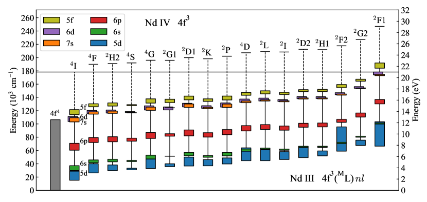
Figure 1: Gross structure of the singly excited system of Nd III, $4\text{f}^{3}(^{\text{M}}\text{L})nl$, up to $nl=\text{5f}$ and relative to the $LS$ terms of the Nd IV ground configuration 4f³. All levels are labeled according to the configurations and parent terms of their leading eigenvector components calculated during the present work using the Cowan code. The extent of each box merely shows the range of level energies within a given $4\text{f}^{3}(^{\text{M}}\text{L})nl$ sub-configuration. The ionisation potential is from Johnson & Nelson (2017) and the Nd IV 4f³ term energies are from Wyart et al. (2007).

The accuracy and availability of atomic data are crucial in the analyses of astrophysical spectra obtained by modern ground and space-based telescopes. The lanthanide elements ($Z=57-71$) are of great interest in the studies of nucleosynthesis, stellar evolution, and Galactic chemical evolution due to their still unsettled origins. Lines from the singly and doubly-ionised lanthanide species are present in spectra of hot chemically peculiar stars in large quantities, see for example, Przybylski’s star (Przybylski, 1977; Cowley et al., 2000). Numerous investigations on AT2017gfo (e.g., Valenti et al., 2017; Coulter et al., 2017), the EM-counter part of neutron star merger event GW170817 (Abbott et al., 2017), indicated large dependence of the kilonova opacity on lanthanide abundances (e.g., Kasen et al., 2013; Tanaka & Hotokezaka, 2013; Smartt et al., 2017; Tanaka et al., 2018; Watson et al., 2019). However, the need for more extensive and accurate heavy element atomic data was almost always emphasised as the limitation to more detailed kilonova modeling. Much effort has been spent to address this by means of large-scale atomic structure calculations of the heavy elements (e.g., Kasen et al., 2013; Fontes et al., 2020; Tanaka et al., 2020). Nevertheless, reliable identification of kilonova spectral features is still hindered by the incompleteness of experimental atomic data and insufficient accuracies of theoretical calculations (Tanaka et al., 2020; Gillanders et al., 2021).

Despite the astrophysical interests in lanthanide spectral data, progress in obtaining accurate experimental energy levels and wavelengths of these elements is slow. Empirical investigations of lanthanide atomic structure are challenging due to their extremely complex and line-rich spectra owing to their $4\text{f}$ valence electrons. Amongst the first few doubly-ionised lanthanide elements, the spectrum of doubly-ionised neodymium (Nd III, $Z=60$) is one of the most poorly known, with only 40 experimental energy levels established previously by Ryabchikova et al. (2006).

In this paper, we address the need for accurate lanthanide atomic data in astronomy, particularly for Nd III, primarily by Fourier transform (FT) spectroscopy of a Penning discharge lamp (e.g., Finley et al., 1979; Heise et al., 1994) between 11500-54000 cm^-1 (8695-1852 Å) using pure Nd cathodes. FT spectroscopy is capable of measuring spectra across a wide spectral range with high spectral resolution, ideal for investigating complex atomic spectra spanning from the IR to UV. At present, FT spectroscopy remains one of the best methods for extensive atomic energy level analysis. Recent examples include: Mn II by Liggins et al. (2021), Ni II by Clear et al. (2022), and Zr I-II by Lawler et al. (2022).

We present the empirical spectrum analysis for 144 energy levels of the $4\text{f}^{4}$, $4\text{f}^{3}5\text{d}$, $4\text{f}^{3}6\text{s}$, and $4\text{f}^{3}6\text{p}$ configurations of Nd III, 39 of 40 previously published energy levels were confirmed and 105 energy levels were established for the first time. In total, 433 Nd III transitions were observed in the FT spectra with uncertainties down to a few $10^{-3}$ cm^-1. We also aim to provide insight into how accurate and extensive lanthanide atomic data was obtained using existing spectroscopic techniques. This research were substantially aided by FT spectroscopy of a Nd hollow cathode discharge, grating spectroscopy of Nd vacuum sliding sparks and Nd-rich stars, consideration of Nd energy level isotope shifts, and calculations using the Cowan code (Cowan, 1981; Kramida, 2021) parameterised by newly established energy levels.

2 Energy Level Structure of Nd III

2.1 Background

Nd III is of the neutral cerium isoelectronic sequence, with even-parity ground configuration [Xe] $4\text{f}^{4}$ and singly excited configurations [Xe] $4\text{f}^{3}nl$. Figure 1 shows a schematic diagram of Nd III energy levels of singly excited configurations up to $nl=\text{5f}$, grouped by parent terms of the 3-electron core under the LS-coupling scheme - $4\text{f}^{3}(^{\text{M}}\text{L})nl$. Transitions and levels involving the ground configuration and $nl=\>$5d, 6s, 6p are the focus of this paper. The primary difficulty of investigating Nd III atomic structure had been, and still remains to be, disentangling the immense number of spectral lines, particularly those of the 4f⁴ - 4f³5d transitions, as the 4f³5d configuration is associated with hundreds of energy levels. In the visible-UV spectral region of the Nd discharge lamps, the 4f⁴ - 4f³5d lines of Nd III also coincide with the complex spectra of Nd I and Nd II due to the low ionisation potentials of Nd. In most cases, empirical atomic structure investigations of the lanthanides require more extensive experimental methodology and data, and more labour intensive spectral analyses, compared to those of the lighter and less complex atoms with open subshells in the $l=\text{s},\text{p},\text{d}$ orbitals.

2.2 Previous Experiments

The first experimental investigations of Nd III atomic structure were by Dieke et al. (1961) and Dieke & Crosswhite (1963) using grating spectroscopy of spark discharges. This led to an unpublished establishment of 29 levels by H. M. Crosswhite, she had provided them for the Martin et al. (1978) compilation and they are found in the NIST database. The 29 levels account for classified transitions from 24 levels of $4\text{f}^{3}5\text{d}$ to all 5 levels of the ground term $4\text{f}^{4}(^{5}\text{I})$, which were likely deduced from isolating Nd III lines by comparing spectra of discharges at various temperatures (Dieke et al., 1961). H. M. Crosswhite’s unpublished lists of 314 classified Nd III lines and 643 lines identified as belonging to Nd III also circulate within the astrophysical community, and the latter proved useful for the present work. Ryabchikova et al. (2006) later proposed revisions for 13 of the 29 levels and classifications for 11 brand new levels of the $4\text{f}^{3}5\text{d}$ configuration, based on stellar spectroscopy, parameterised Cowan code calculations and Fourier transform spectroscopy of Nd hollow cathode discharges by Aldenius (2001).

2.3 Energy Level Calculations

Theoretical calculations of atomic structure and transition probabilities are invaluable in the experimental establishment of energy levels and classification of observed spectral lines. Bord (2000), Zhang et al. (2002), and Dzuba et al. (2003) published the first theoretical investigations of the Nd III spectrum, all utilising the Cowan code (Cowan, 1981). Eigenvector compositions of the 4f³5d levels below 33000 cm^-1 were published by Zhang et al. (2002) and Ryabchikova et al. (2006) under the LS-coupling scheme. Gaigalas et al. (2019) and Silva et al. (2022) published calculations for many more higher-lying levels and configurations, and the readily available online data from Gaigalas et al. (2019) for level energies, leading LS term labels, and transition probabilities proved useful during the initial stages of the present empirical spectrum analysis of Nd III.

More accurate calculations of energy level values, level eigenvector compositions, and transition probabilities were required in the search for the experimentally unknown levels of Nd III in the present work. The Cowan code (Cowan, 1981; Kramida, 2021) was shown suitable for this purpose. The configuration interaction space consisted of the even parity configurations 4f⁴ + 4f²5d² + 4f³6p + 4f³5f and the odd parity configurations 4f³5d + 4f³6s + 4f³7s + 4f³6d + 4f²5d6p. First, the calculations were performed in the ab initio pseudo-relativistic Hartree-Fock (HFR) approximation with scaling factors of the Slater and configuration interaction parameters set at 0.85 and 0.70 respectively. To account for the incomplete interaction space, the Slater parameters and additional energy parameters $\alpha$, $\beta$, and $\gamma$ were then adjusted from considering calculations from Ryabchikova et al. (2006) for Nd III and from the calculations of the neighbouring spectra of Pr II (Mashonkina et al., 2009), Pr III (Palmeri et al., 2000; Wyart et al., 2010, unpublished calculations), Nd II (Wyart, 2010; Wyart et al., 2010, unpublished calculations), and Nd IV (Wyart et al., 2007). The energy parameters were adjusted in an iterative process by fitting newly established experimental energy levels when they became available during the empirical spectrum analysis.

The final energy parameters calculated for the 4f⁴, 4f³5d, 4f³6s, and 4f³6p configurations are listed in Table 1, remaining parameters are included in the machine-readable version online. The number of experimental levels was insufficient to fit all energy parameters; $\alpha$, $\beta$, and $\gamma$ were fixed at their estimated values for all configurations to allow the maximum number of Slater parameters to be fitted. There were enough core terms for all three F^2,4,6(4f,4f) electrostatic parameters only for the 4f³5d configuration. It was possible to fit the levels of the 4f⁴, 4f³6p and 4f³5f configurations with free F²(4f,4f) and F⁴(4f,4f) parameters and fixed F⁶(4f,4f) parameter at the 0.852 ratio (Fitted/HFR) obtained for the 4f³5d configuration. Only one core term (⁴I) was available for the 4f³6s, 4f³7s, and 4f³6d configurations, the F^2,4,6(4f,4f) of these configurations, and of the doubly-excited configurations 4f²5d² and 4f²5d6p, were fixed at their ratios obtained for the 4f³5d configuration.

Table 1: Parameters of the least-squares fit of energy levels of the 4f⁴, 4f³5d, 4f³6s, and 4f³6p configurations of Nd III of Cowan’s codes.

Conf.	Param.	LSFa	Gb	HFRa,c	Ratioa,d
		(cm-1)		(cm-1)
4f4	$E_{\text{av}}$	32348(22)		35503	-3156
	F2(4f,4f)	71335(105)		92636	0.770
	F4(4f,4f)	40755(201)		57680	0.707
	F6(4f,4f)	35267(f)	3	41372	0.852
	$\alpha$(4f)	8(f)		0
	$\beta$(4f)	-310(f)		0
	$\gamma$(4f)	1110(f)		0
	$\zeta$(4f)	782(4)		849	0.921
4f35d	$E_{\text{av}}$	44999(43)		36770	8229
	F2(4f,4f)	78070(397)	1	101378	0.770
	F4(4f,4f)	49616(383)	2	63552	0.781
	F6(4f,4f)	38949(554)	3	45705	0.852
	$\alpha$(4f)	22(f)		0
	$\beta$(4f)	-600(f)		0
	$\gamma$(4f)	1450(f)		0
	$\zeta$(4f)	882(2)	4	947	0.932
	$\zeta$(5d)	785(7)		831	0.945
	F1(4f,5d)	953(81)		0
	F2(4f,5d)	19310(119)		26408	0.731
	F3(4f,5d)	0(f)		0
	F4(4f,5d)	13958(275)		13022	1.072
	G1(4f,5d)	9138(39)		12824	0.713
	G2(4f,5d)	1689(198)		0
	G3(4f,5d)	9205(142)		10202	0.902
	G4(4f,5d)	0(f)		0
	G5(4f,5d)	5148(126)		7735	0.666
4f36s	$E_{\text{av}}$	55647(49)		47956	7691
	F2(4f,4f)	78723(400)	1	102226	0.770
	F4(4f,4f)	50064(387)	2	64126	0.781
	F6(4f,4f)	39310(559)	3	46129	0.852
	$\alpha$	22(f)		0
	$\beta$	-600(f)		0
	$\gamma$	1450(f)		0
	$\zeta$(4f)	886(2)	4	953	0.932
	G3(4f,6s)	2393(72)		2870	0.834
4f36p	$E_{\text{av}}$	88343(29)		79811	8544
	F2(4f,4f)	78655(146)		102329	0.769
	F4(4f,4f)	49923(164)		64196	0.778
	F6(4f,4f)	39344(f)	3	46180	0.852
	$\alpha$(4f)	22(f)		0
	$\beta$(4f)	-600(f)		0
	$\gamma$(4f)	1450(f)		0
	$\zeta$(4f)	888(2)		954	0.930
	$\zeta$(6p)	2467(10)		1989	1.240
	F1(4f,6p)	739(45)		0
	F2(4f,6p)	6396(359)		7861	0.814
	G2(4f,6p)	2082(55)		1981	1.051
	G3(4f,6p)	0(f)		0
	G4(4f,6p)	1490(93)		1791	0.832

Note. —

^a Parameter values determined in the ab initio pseudo-relativistic Hartree–Fock (HFR) and least-squares-fitted (LSF) calculations and their ratio. Standard deviation of the fitted LSF parameters are in brackets, where ‘f’ means the parameter is fixed.

^b Group of the parameter, where parameters in each numbered group were linked together by sharing the same ratios to their corresponding HFR values.

^c The average energies were adjusted so that the energy of the ground level 4f^{4 5}I₄ is zero in the HFR calculations with scaling of the Slater and configuration interaction parameters by factors of 0.85 and 0.70 respectively.

^d Differences between LSF and HFR parameters are given for $E_{\text{av}}$.

(This table is available in its entirety in machine-readable form)

Level energies of the 4f²5d² and 4f²5d6p configurations overlap greatly with other configurations. Corresponding configuration interactions may affect calculated level energies and transition probabilities, especially in cases of close proximity to particular levels. Regrettably, no level was established in these doubly-excited configurations, and their energy parameters were adjusted only using information from neighbouring ion spectra and from the other Nd III configurations. It should be noted that the estimated energies of the lowest ⁵L₆ levels in the 4f²5d² and 4f²5d6p configurations, 72827 and 126176 cm^-1 respectively, are in agreement with those predicted by Brewer (1971) at 72000$\pm$2000 and 126000$\pm$4000 cm^-1.

Using the energy and configuration interaction parameters from Table 1, the standard deviations of the predicted level energies from their experimental values were 29 and 36 cm^-1 for the even and odd level systems respectively. Corresponding level eigenvector compositions and transition probabilities were also calculated. In searching for experimentally unknown energy levels, these calculations addressed the insufficient accuracy in the theoretical predictions by Gaigalas et al. (2019), particularly for higher-lying energy levels at higher level densities.

3 Experimental Details

3.1 Fourier Transform Spectroscopy of Nd

All level energies within this publication were determined using spectral lines measured by the high-resolution f/25 Imperial College VUV FT spectrometer (Thorne et al., 1987), using a custom-built water-cooled Penning discharge lamp (PDL), designed by Heise et al. (1994), with 99.5% pure Nd cathodes (natural isotope abundances), a magnesium fluoride window, and argon as the sputtering carrier gas. The 0.5% impurities in the cathodes were primarily iron and praseodymium, however, no known lines of these species were observed. Stable lamp running pressures and currents were chosen such that the signal-to-noise ratios (SNRs) of the previously classified known Nd III transitions were maximised, which were (1.7-2.4)$\times 10^{-3}$ mbar and 650-750 mA respectively. The discharge remained stable for 2-3 hours under these conditions before the Nd cathodes were depleted. The PDL was chosen as the light source for its lower pressure and higher temperature stable discharge giving higher Nd III populations, compared to those produced by the alternative hollow cathode discharge lamp commonly used in FT spectroscopy. As far as we know, no previous records on producing Nd spectra using a PDL light source have been published previously.

Table 2: Nd-Ar PDL FT spectra parameters.

Spec.	Spec. Range	Res.	Pressure	Current	No. of	Photomult.	Optical	Int. Calib.	$k$eff
	(cm-1)	(cm-1)	($10^{-3}$ mbar)	(mA)	Co-adds	Tube	Filter	Lamp	($10^{-7}$)
(1)	(2)	(3)	(4)	(5)	(6)	(7)	(8)	(9)	(10)
A	11890-17687	0.045	1.7	750	8	R928	OG530	W	1.74 $\pm$ 0.14
B	17687-21300	0.050	2.2	750	7	R11586	GG475	W	1.39 $\pm$ 0.09
C	21300-25369	0.050	2.3	650-750	19	R11586	GG385+SP500	W	-3.10 $\pm$ 0.20
D	25369-32480	0.055	2.4	750	21	R11586	UG5-C	W	-2.95 $\pm$ 0.12
E	32480-44422	0.070	1.7	750	23	R7154	-	D2	-2.88 $\pm$ 0.19
F	44422-53822	0.080	2.0	750	32	R8486	180-B-1D	D2	-4.32 $\pm$ 0.38

Note. — Column (1) is the spectrum name, column (2) is the spectral range within which the corresponding transitions were measured, column (3)-(5) are the spectral resolution, running pressures and currents respectively, column (6) is the number of interferogram co-adds, and columns (7)-(9) are the detector, filter, and intensity calibration lamp used respectively, W indicates tungsten lamp and D₂ indicates deuterium lamp. The final column lists the wavenumber calibration factors and their uncertainties.

Nd-Ar PDL FT spectra were recorded in six separate spectral regions within 11500-54000 cm^-1 (8695-1852 Å). Spectral ranges spanning the visible were narrower (in cm^-1) compared to the UV regions, this was to reveal weaker lines by reducing photon noise from the intense and numerous Nd I-III lines in the visible. Spectral resolving power was limited by predominantly the Doppler line widths as no instrumental ringing was observed. Observed spectral lines from all 6 spectra were fitted to create a line list used in the energy level search. Most lines were fitted using the Voigt profile, where the Lorentzian components of the line widths were observed to be around one order of magnitude smaller than the Gaussian (Doppler) components. The statistical uncertainty in the wavenumber $\sigma_{\text{obs}}$ of a spectral line estimated by Voigt profile fitting is (Davis et al., 2001)

$$\Delta\sigma_{\text{obs}}=\frac{1}{\sqrt{N}}\frac{\text{FWHM}}{\text{SNR}},$$ (1)

where $N$ is the number of points within the full width at half maximum $\text{FWHM}$, and $\text{SNR}$ was capped at 100 to prevent unrealistically low uncertainties. Details regarding non-Voigt profile spectral line fitting will be discussed in section 4.3.

Experimental details of the six Nd-Ar PDL FT spectra, labeled alphabetically, are listed in Table 2. The final column lists wavenumber calibration factors $k$_eff of observed wavenumbers $\sigma$_obs in each spectrum, where the calibrated wavenumbers $\sigma$_cal are defined by (Haris & Kramida, 2017):

$$\sigma\textsubscript{cal}=(1+k\textsubscript{eff})\sigma\textsubscript{obs}.$$ (2)

This calibration factor mainly accounts for the finite aperture size of the FT spectrometer and any misalignment of the lamp and the spectrometer’s calibration laser (Learner & Thorne, 1988). Wavenumber calibration was carried out using 13 of the 28 Ar II reference lines recommended by Learner & Thorne (1988) within spectrum C, using their corresponding reference wavenumbers measured by Whaling et al. (1995). The remaining Ar II reference lines in spectrum C were unsuitable due to low SNRs and/or blending with Nd lines.

A calibration factor $k_{\text{eff},i}$ was determined for each reference wavenumber $\sigma_{\text{cal},i}$ in a spectrum using its observed wavenumber in (2), and then the $k_{\text{eff}}$ of the spectrum was the weighted average

$$k_{\text{eff}}=\frac{\sum_{i}w_{i}\,k_{\text{eff},i}}{\sum_{i}w_{i}},$$ (3)

with weights $w_{i}=(\Delta k_{\text{eff},i})^{-2}$, where the $\Delta k_{\text{eff},i}$ were the absolute uncertainties of $k_{\text{eff},i}$ determined by (2). The uncertainty in the calibration factor $k_{\text{eff}}$ was given by (Radziemski & Andrew, 1965; Haris & Kramida, 2017)

$$\Delta k_{\text{eff}}=\frac{\sqrt{\sum_{i}[w_{i}+w_{i}^{2}(k_{\text{eff}}-k_{\text{eff},i})^{2}]}}{\sum_{i}w_{i}}.$$ (4)

The systematic uncertainties $\Delta\sigma_{\text{sys}}$ in wavenumber calibration are given by $\sigma\textsubscript{obs}\Delta k\textsubscript{eff}$, which were added in quadrature with $\Delta\sigma_{\text{obs}}$ from (1) to yield the final wavenumber uncertainty for each line.

The above was repeated for each of the other spectra by using calibrated lines within overlapping spectral regions as wavenumber references. These were selected from lines that were non-blended, at intermediate SNRs, and with no evidence of self-absorption in their fit residuals. In this procedure, the $\Delta\sigma_{\text{sys}}$ of each other spectrum could become lower than that of spectrum C, e.g. low RMS residuals of $k_{\text{eff},i}$, higher SNRs and/or a larger number of reference lines $i$. This was addressed by conservatively estimating the systematic uncertainty of a spectrum to be a linear sum including all previous systematic uncertainties, e.g.,

$$\Delta\sigma_{\text{sys}}^{\text{F}}=\Delta\sigma_{\text{sys}}^{\text{F}}+\Delta\sigma_{\text{sys}}^{\text{E}}+\Delta\sigma_{\text{sys}}^{\text{D}}+\Delta\sigma_{\text{sys}}^{\text{C}},$$ (5)

where the values from previous spectra were from overlapping spectral regions. This procedure was later verified by the lack of any systematic offsets seen between the observed and Ritz wavenumbers of transitions from energy levels with transitions across multiple spectra (Ritz wavenumbers are the differences between level energies optimised using all observed wavenumbers, see Section 5.1.1 for details). Differences between all observed and Ritz wavenumbers also lay within 1.2 times the estimated final wavenumber uncertainties, which were no more than 0.003 cm^-1 ($\sim$0.0003 Å at 3000 Å) for unblended lines with SNR $>$100 and free from self-absorption.

All six Nd-Ar PDL FT spectra were intensity calibrated using either a tungsten standard lamp (IR to UV) or a deuterium standard lamp (UV to VUV). Intensities measured in different spectral regions were placed onto a common relative intensity scale set by spectrum C, using lines within overlapping regions of neighbouring spectra. When possible, only known Nd III lines were used. The observed relative line intensities from this work are recommended as only a rough guide, especially when comparing intensities between the different spectral regions listed in Table 2.

Spectra of a custom-built water-cooled hollow cathode discharge lamp (HCL) with the identical 99.5% Nd cathode composition were also recorded using Ar carrier gas, with similar numbers of co-adds and the identical six spectral ranges, detectors, filters, and intensity calibration lamps listed in Table 2, but at higher resolutions due to the narrower Doppler line widths of the HCL spectral lines. Stable conditions were chosen to maximise the SNRs of previously classified Nd III transitions at 0.43 mbar and 450 mA running pressure and current respectively. Under these conditions, the HCL ran stably for experiments over many weeks of use until cathode depletion. The HCL spectra were only used in this work as a guide for line intensities from a Nd-Ar plasma at a lower effective temperature compared to the Nd-Ar PDL plasma.

3.2 Grating Spectroscopy of Nd

Two sets of spectra of Nd vacuum sliding sparks (VS) of currents up to 1500 A were used for the analysis of Nd III atomic structure. The spectra in the 390-1525 Å and 1600-2536 Å ranges were taken on the 6.65 m normal incidence spectrometer at the Institute of Spectroscopy in Troitsk. The spectrometer is equipped with a 1200 lines/mm grating providing a 1.25 Å/mm plate factor. The spectra were recorded on Ilford Q photographic plates and measured on the automatic comparator with a scanning step of 0.3 µm controlled by the system for the automatic processing of photo-spectrograms designed by Azarov (1991). The other set of spectra consists of photographic plates from NIST, recorded on the 10 m normal incidence spectrograph and covered 2330-3250 Å. These spectra were scanned by an Epson Expression 1000 XL scanner, and the spectral line positions and intensities were measured using the GFit code (Engström, 1998).

Impurity lines of oxygen, carbon, nitrogen, and silicon in various ionisation stages (Kramida et al., 2022), as well as lines of Nd IV (Wyart et al., 2007) and Nd V (Meftah et al., 2008), were used for wavelength calibration initially. After the measurement and classification of Nd III lines by FT spectroscopy in this work, the Nd VS grating spectra were calibrated again with the addition of the Nd III Ritz wavelengths. The final uncertainties of unblended and symmetric lines of moderate intensity were estimated at 0.006 Å.

In contrast to the HCL spectra, the Nd VS grating spectra were a guide for relative line intensities at higher effective temperatures compared to the PDL. Furthermore, these grating spectra also contained weaker Nd III lines that were absent in the Nd-Ar PDL spectra.

3.3 Stellar Spectroscopy of Nd

The laboratory analysis of the Nd III spectrum was also supplemented by the analysis of high-resolution, high SNR spectra of the magnetic chemically peculiar Ap stars with large atmospheric Nd overabundance. Two tepid stars of similar atmospheric parameters (effective temperature and surface gravity) but different surface magnetic fields were chosen: HD 170973 with $T_{\rm eff}$=11200 K, $\log g$=3.8 (Ryabchikova et al., 2011) and HD 144897 with $T_{\rm eff}$=11250 K, $\log g$=4.0 (Ryabchikova et al., 2006). The spectra of both stars ranged from 3030 to 10400 Å and were recorded at resolving power R=80 000 by the UVES instrument at the ESO VLT under the program 68.D-0254. More details of the observations and spectrum reduction are given in Ryabchikova et al. (2008). The surface magnetic field $\langle B_{\rm s}\rangle$=8.8 kG in HD 144897 was estimated from Zeeman splitting of spectral lines (Ryabchikova et al., 2006), while the absence of any splitting in spectrum of HD 170973 together with one estimate of the longitudinal magnetic field $\langle B_{\rm z}\rangle$=392$\pm$5 G (G. Wade, private communication) did not indicate the presence of a surface magnetic field stronger than 1 kG in the atmosphere of HD 170973. Both stars rotate slowly with projected rotational velocity $v_{\rm e}\sin i$=8.5 km s^-1  (HD 170973) and $v_{\rm e}\sin i$=3 km s^-1  (HD 144897).

The atmospheres of the two stars are very rich in rare-earth elements, their average Nd abundances exceed the solar value by four orders of magnitude. In the solar photosphere, $\log\varepsilon_{\rm Nd}$=1.42 (Lodders, 2021), whereas $\log\varepsilon_{\rm Nd}$=5.39$\pm$0.18 for HD 170973 (Kato, 2003). In the present work, the reference Nd abundance of HD 170973 was recalculated at 5.63$\pm$0.14 using $T_{\rm eff}$=11200 K, $\log g$=3.8 (Ryabchikova et al., 2011), and equivalent widths of 30 Nd III lines previously classified by Ryabchikova et al. (2006) and observed in the Nd-Ar PDL FT spectra. The reference abundance for HD 144897 was estimated at $\log\varepsilon_{\rm Nd}$=5.59$\pm$0.20 (Ryabchikova et al., 2006). The temperatures, high Nd abundances, and differing surface magnetic field strengths of the two stars favoured the careful analysis of Nd III lines in their spectra.

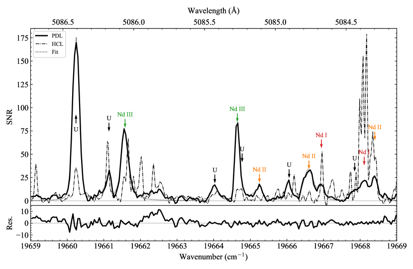
Figure 2: Emission spectrum of Nd recorded using Fourier transform spectroscopy between 19659-19669 cm^-1 (vacuum) containing lines with intermediate signal-to-noise ratios and showing weak and uncertain blended spectral lines. Penning discharge lamp (PDL) and hollow cathode lamp (HCL) spectra are solid and dash-dotted lines respectively. The dotted line shows fits to the 13 lines identified in the PDL spectrum, residuals are shown at the bottom. Lines identified and fitted in the PDL spectrum are indicated by vertical arrows and labels, those with label U are unclassified.

4 Spectrum of the Nd Penning Discharge Lamp

4.1 Spectrum and Line Identification

A total of 21584 lines were identified and fitted in the Nd-Ar PDL FT spectra by the peak-finding algorithm of Nave et al. (2015) and by manual fine-tuning. The line list contained transitions of Nd I-IV and Ar I-III and the numbers of observed known lines of each species are listed in Table 3. Apart from Nd III, the number of classified lines of each other species is uncertain due to the large quantity of unidentified blended and weak lines. For Nd I and Nd II, a significant number of matches with Ritz wavenumbers are expected to be coincidental and incorrect. Moreover, many levels from the NIST database are also uncertain with only configuration and $J$ value assignments. Figure 2 highlights the difficulties and uncertainties of line identification with a 10 cm^-1 section of the Nd FT spectrum, measured in both the PDL and HCL and representative of the most line-rich and intense regions 15000-30000 cm^-1 (6666-3333 Å), where a large fraction of the Nd III 4f⁴ - 4f³5d, Nd I, and Nd II transitions lie.

Table 3: Species and lines identified in Nd-Ar PDL FT spectra.

Species	No. of Linesa	Line List for Identification
Nd I	1636	NIST ASDb
Nd II	6574	NIST ASDb
Nd III	580c	This work
Nd IV	54	Wyart et al. (2007)
Ar I	48	Whaling et al. (2002)
Ar II	430	Saloman (2010)
Ar III	90	Saloman (2010)

Note. —

^a Number of lines whose wavenumbers matched known lines within $\pm 0.2$ cm^-1 for Nd IV, and $\pm 0.05$ cm^-1 for the other species.

^b Using Ritz wavenumbers allowed by $\Delta J=0,\pm 1$, but not $J=0\leftrightarrow 0$ and parity selection rules for E1 transitions of the energy levels that were mostly from Martin et al. (1978); Blaise et al. (1971, 1984).

^c 147 of these lines belong to the 4f³6p - 4f³7s and 4f³6p - 4f³6d transitions, which will be reported in a future publication.

Weak lines and weak blends such as the feature at 19662.5 cm^-1 of the PDL spectrum in Figure 2 were often missed by the peak finding algorithm and manual fine-tuning when fitting line profiles for the line list. The labour cost of analysing and fitting every single line around the noise level was considered not feasible due to their ubiquity and large uncertainties from high susceptibility to blending. For example, in the comparison between the PDL and HCL spectra of Figure 2, all 13 PDL lines of the 10 cm^-1 section were arguably blended to some extent. The incompleteness and inaccuracy of the list of observed wavenumbers were two of the most limiting factors in the empirical search for energy levels; expected transitions may be missing in the line list due to weak and unfitted lines or inaccurately fitted blends. Around 2000 of the 21559 lines were in fact fitted later during the empirical Nd III energy level analysis when more thorough spectrum fitting of blends and weak lines became necessary within spectral regions containing weak Nd III transitions of interest.

The primary assistance in line and blend identification was provided by the HCL spectra, which produced an Nd-Ar discharge at a lower temperature with narrower Doppler widths (this is more conveniently seen in the upper plot of Figure 3). Lines of Nd I could also be identified with reasonable certainty, as Nd I was the only Nd species with reduced relative intensities in the PDL compared to that of the HCL, and this is noticeable in Figure 2. Self-absorption was observed in the PDL for a fraction of Nd II transitions between the lowest-lying levels, evident from the self-reversals, flattened tops, or most commonly the reversed ‘W’ Voigt profile fit residuals of these line profiles. The line in Figure 2 at 19660.2 cm ^-1 was unclassified but showed features of self-absorption, indicating the possibility of it being an unclassified Nd II transition.

Compared to the line-rich visible-UV regions, the Nd-Ar PDL spectrum was relatively much less intense in the deeper UV (30000-50000 cm^-1, 3333-2000 Å) and was not plagued by a large number of blended and weak lines. This indicated lower populations of Nd III ions at the 4f³6p, 4f³7s, 4f³6d and doubly excited configurations, and of Nd IV ions at the 4f²5d and 4f²6p configurations; their transitions to lower levels were expected in this region but were observed at low SNRs. The lines with the highest SNRs in this region were the 4f^4 5I - 4f³(⁴G)5d transitions of Nd III around 35500 cm^-1.

4.2 Nd III Isotope Shifts

Many Nd lines of the FT spectra showed similar non-Voigt line profiles despite the likelihood of line blending. The cathodes of the PDL and HCL contained natural abundances of the 7 stable isotopes (Berglund & Wieser, 2011): Nd-142 (27.15%), Nd-143 (12.17%), Nd-144 (23.80%), Nd-145 (8.29%), Nd-146 (17.19%), Nd-148 (5.76%), and Nd-150 (5.64%), all of which have non-negligible abundance. Energy levels of Nd-143 and Nd-145 also have hyperfine structure. Consideration of isotope shifts of different transition arrays was a key component in the empirical atomic structure analyses of Nd I and Nd II (e.g., Blaise et al., 1971, 1984; Wyart, 2010). Likewise, isotope line profiles of the 4f⁴ - 4f³5d Nd III transitions were indispensable for their classifications in this work.

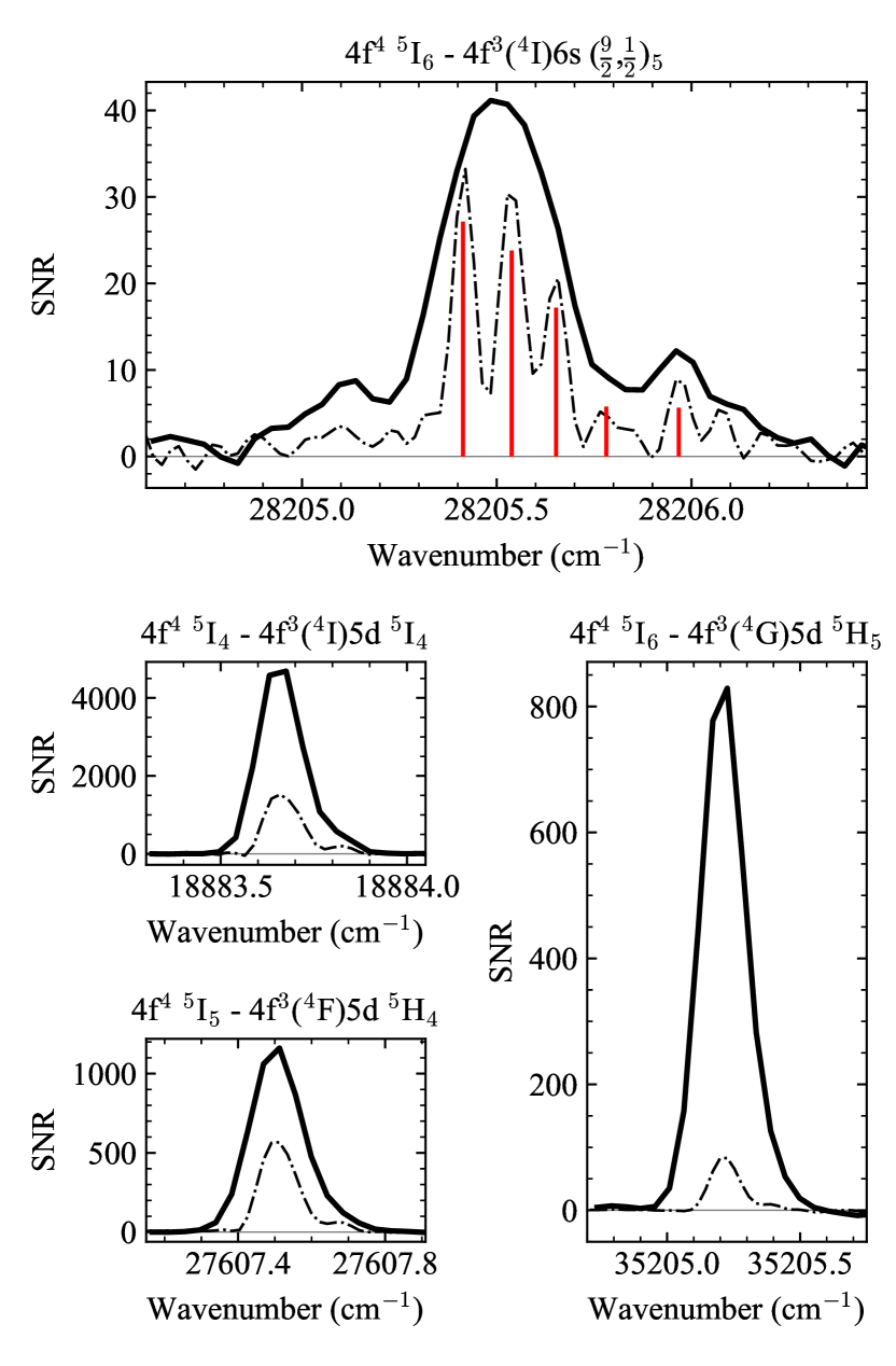
Figure 3: Isotope structure of 4 Nd III lines observed by Fourier transform spectroscopy of the Nd-Ar Penning discharge lamp (PDL, solid) and the Nd-Ar hollow cathode lamp (HCL, dash-dotted). For 4f^4 5I₆ - 4f³(⁴I)6s $(\frac{9}{2},\frac{1}{2})_{5}$, isotope components of Nd-142, Nd-144, Nd-146, Nd-148, and Nd-150 are marked tentatively from left to right with red vertical lines in relative abundance ratios from Berglund & Wieser (2011), remaining features are likely hyperfine structures of Nd-143 and Nd-145 or blended weak lines.

Observations of Nd III isotope structure were first made by Aldenius (2001). Examples observed in the FT spectra of the present work are shown in Figure 3. The transition 4f^4 5I₆ - 4f³(⁴I)6s $(\frac{9}{2},\frac{1}{2})_{5}$ was the only Nd III line observed in the HCL spectrum with resolved Nd-142, Nd-144, and Nd-146 isotope components. The Nd-148 and Nd-150 components at higher wavenumbers are uncertain due to smaller relative abundances, low SNRs, and hyperfine structure of the Nd-143 and Nd-145 isotopes. This pattern was a reflection of, but consistent with, many isotope profiles observed for Nd I (e.g., 19668.1 cm^-1 of Figure 2) and Nd II (e.g., Figure 2 of Koczorowski et al., 2005). Isotope shifts added another layer of complexity in line identification; in Figure 2, the unclassified line of 19667.9 cm^-1 was possibly misidentified as an individual line rather than a part of the isotope structure of the Nd I line. Almost all classified 4f⁴ - 4f³5d transitions of Nd III showed an unresolved Nd-150 right-side wing within the PDL spectra (e.g., see Figure 3), which was an essential clue to their classification when observed at a sufficient SNR.

4.3 Line Profile Fitting

Least-squares fitting using the Voigt profile was not suitable for all the observed PDL spectral line profiles. Lines showing significant isotope structure were fitted by using the centre-of-gravity (COG) wavenumber, i.e., an average of wavenumbers within a manually specified range weighted by SNR. For COG fitted lines, statistical uncertainties from equation (1) were doubled. However, the unresolved Nd-150 right-side wings of the 4f⁴ - 4f³5d Nd III transitions were not always obvious during visual inspections and manual corrections to the output of the peak-finding algorithm, particularly at intermediate and lower SNRs. In this case, not only would the isotope shift clue be lost, but the differences between wavenumbers from Voigt and COG fits were often larger than their statistical uncertainties. This again caused inaccuracies of wavenumbers in the line list, which obstructed the search for Nd III energy levels. Additionally, COG fitting may not be as accurate for blended and weak lines, as specifying wavenumber limits of such line profiles could range from non-trivial to impossible.

Instead, an asymmetric Voigt profile was used to quantify the unresolved Nd-150 right-side wings of the 4f⁴ - 4f³5d transitions, and to more accurately estimate wavenumbers of similarly asymmetric line profiles. The dominant Doppler width of the Voigt profile $w$ was varied as a sigmoid function of wavenumber parameterised by an asymmetry factor $a$ (Stancik & Brauns, 2008),

$$w(\sigma)=\frac{2w_{0}}{1+e^{a(\sigma-\sigma_{0})}},$$ (6)

where $w_{0}$ and $\sigma_{0}$ are the Doppler width and wavenumber of the usual Voigt profile ($a=0$) respectively. The wavenumber of the fitted line was estimated using the COG of this asymmetric Voigt profile. Lines resembling the Nd-150 right-side wing asymmetry would have $a<0$.

By no means was this asymmetric Voigt profile an accurate physical description of isotope shifts, but overall improvements in wavenumber fitting were achieved for the 4f⁴ - 4f³5d transitions. In the example shown in Figure 4, the choice of COG wavenumber limits was difficult due to slight blending with a second weaker line, the unresolved right wing was not obvious from inspection and only evident from Voigt fit residuals. When fitted using the Voigt profile, the observed wavenumber differed from Ritz and asymmetric Voigt fit values by more than the wavenumber uncertainty. The example in Figure 4 was fitted with $a=-1.62$. Statistical uncertainties from equation (1) were doubled for any lines with $|a|>1$, and $a$ was fixed at 0 for lines with SNRs lower than 10.

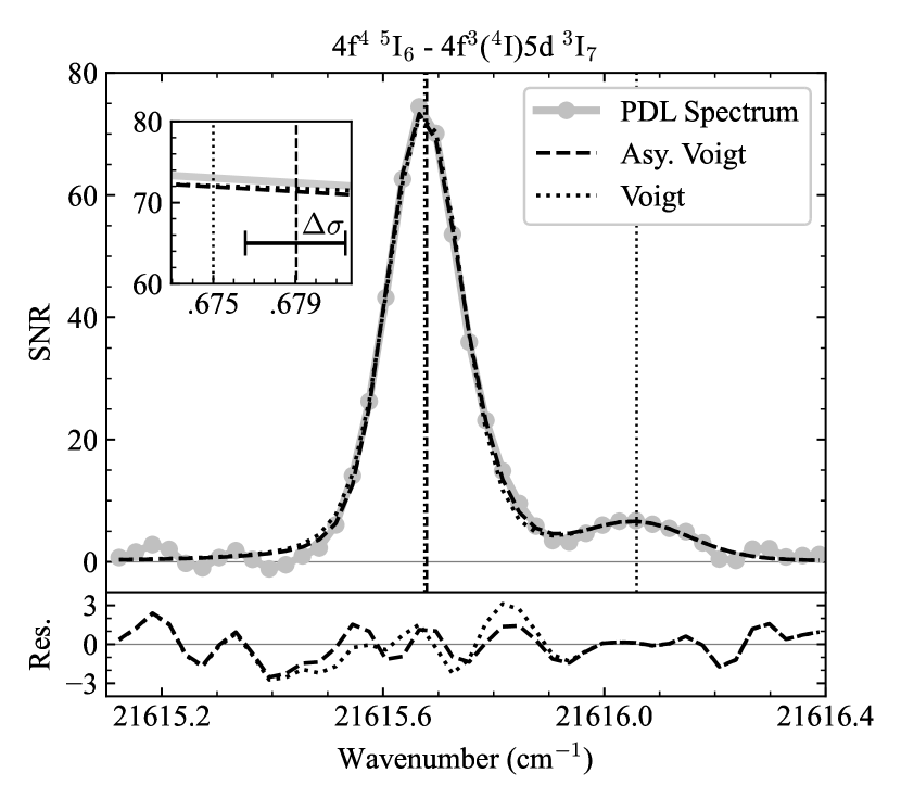
Figure 4: Nd III transition 4f⁴(⁵I₆) - 4f³(⁴I)5d ³I₇ at 21615.679 cm^-1, slightly blended with an unclassified line at 21616.058 cm^-1. Fits using asymmetric Voigt and normal Voigt profiles are shown in dashed and dotted lines respectively, their residuals are shown in the lower plot and their fitted wavenumbers are shown by the vertical lines. The wavenumber uncertainty of the asymmetric Voigt fit $\Delta\sigma$ is shown in the zoomed section.

Compared to using the normal Voigt function, wavenumbers from asymmetric Voigt fits were closer to and within uncertainties of manual COG values. This fitting method also alleviated a prohibitive amount of labour otherwise induced by manually specifying limits of COG wavenumbers of thousands of such lines. Flexible adjustments of the line list using all 3 line fitting methods were readily available using a custom computer program, where each line (row) of the line list contained the essential parameters (columns): SNR, FWHM, calibrated wavenumber (Voigt or COG) and its final uncertainty, calibrated relative intensity, method of fitting, and the asymmetry factor $a$.

5 Empirical Spectrum Analysis of Nd III

Initially, results from previously published experimental investigations of Nd III were used to classify Nd III lines, and then unclassified lines were used in the search for new energy levels using theoretical calculations as a guide. The methodology is discussed in more detail in Section 5.2.

5.1 Results

5.1.1 Energy Levels

Wavenumbers of classified Nd III transitions from the Nd-Ar PDL FT spectra were input into the program LOPT (Kramida, 2011) to estimate the optimum level energies and Ritz wavenumbers by minimisation of the squared difference between observed wavenumbers and their Ritz values. These observed wavenumbers were calibrated onto the same absolute scale, but systematic wavenumber shifts (below the systematic uncertainties) still remain between each spectrum. Initially, the systematic shifts of wavenumbers from each spectrum were assumed zero for the input of LOPT, and systematic uncertainties from calibration were only included as a part of the weights in the best fit by LOPT, therefore risking underestimation of calibration uncertainties for the Ritz wavenumbers. To address this, the systematic uncertainties $\Delta\sigma_{\text{sys}}$ from the six spectra were added in quadrature (yielding $\pm 0.0052$ cm^-1) and then in quadrature with all Ritz wavenumber uncertainties determined by LOPT for a more conservative estimate of line and level energy Ritz wavenumber uncertainties.

The experimentally established energy levels of the 4f⁴, 4f³5d, 4f³6s, and 4f³6p configurations of Nd III from this work are listed in Table 4 in order of ascending energy of their assigned configurations and terms. Pure LS-coupling basis functions were used to label energy levels of the 4f⁴, 4f³5d and 4f³6p configurations. Under this scheme, purity is high overall for the lowest-lying terms of the 4f⁴ and 4³5d configurations. Higher-lying levels of these two configurations, and the 4f³6p levels, were mixed; violation of the LS-coupling selection rules (i.e., $\Delta S=0$ and $\Delta L=0,\pm 1$ but not $L=0\leftrightarrow 0$) was thus very common. For the 4f³(⁴I)6s levels, jj-coupling of the 6s electron with the 4f³(⁴I) core was used for assignment as the basis functions under this coupling scheme better represented their assigned levels.

Table 4: Energy levels experimentally established for the 4f⁴, 4f³5d, 4f³6s, and 4f³6p configurations of Nd III.

Assignment			Energy	$N$	$\Delta E_{1}$	$\Delta E_{2}$	$g$	Eigenvector Composition
Conf.	Term	$J$	(cm-1)		(cm-1)			(%)
4f4	5I	4	0.000(   -)	22(5)	-8	0	0.604	97	4f4 5I	1	4f4 3H4	1	4f4 3H3
		5	1137.794(  5)	31(7)	-3	65	0.901	98	4f4 5I	1	4f4 3H4
		6	2387.544(  6)	34(7)	-4	124	1.071	99	4f4 5I
		7	3714.548(  6)	29(6)	-12	172	1.177	98	4f4 5I	1	4f4 3K2
		8	5093.257(  6)	18(5)	-23	209	1.247	96	4f4 5I	2	4f4 3K2	1	4f4 3K1
4f4	5F	2	10773.962(13)	4(3)	26	-1325	1.007	93	4f4 5F	3	4f4 3D1	1	4f4 3D2
		3	11424.605(  8)	9(1)	23	-1300	1.244	95	4f4 5F	1	4f4 3D1	1	4f4 3F3
		4	12181.327(  7)	13(2)	32	-1279	1.330	92	4f4 5F	3	4f4 3G2	1	4f4 3F3
		5	13210.278(  8)	10(4)	41	-1234	1.387	93	4f4 5F	3	4f4 3G2	1	4f4 3G1
4f4	3K2	6	14064.277(  6)	8(3)	-26	-1002	0.860	78	4f4 3K2	20	4f4 3K1
		7	15153.807(  7)	11(3)	2	-1027	1.005	69	4f4 3K2	18	4f4 3K1	11	4f4 3L
		8	16459.136(  8)	8(5)	66	-1007	1.105	63	4f4 3K2	14	4f4 3K1	11	4f4 3L
4f4	5G	3	15349.601(  6)	5(3)	-1	-2018	0.885	73	4f4 5G	14	4f4 3G2	7	4f4 3G3
		4	16831.344(10)	5(3)	-75	-1944	1.051	69	4f4 5G	13	4f4 3H4	10	4f4 3H3
		5	18313.004(  6)	7(3)	-26	-1825	1.167	57	4f4 5G	18	4f4 3H4	17	4f4 3H3
4f4	3H4	5	16622.337(  7)	7(1)	-11	-1316	1.157	36	4f4 5G	21	4f4 3H4	13	4f4 3H3
4f3(4I)5d	5L∘	6	15158.154(  8)	2(0)	-52	-100	0.724	93	(4I)5d 5L	3	(2H2)5d 3K	3	(4I)5d 3K
		7	16952.835(  8)	2(0)	-29	-32	0.914	97	(4I)5d 5L	2	(2H2)5d 3K	1	(4I)5d 3K
		8	18861.064(  8)	4(1)	-12	26	1.043	99	(4I)5d 5L	1	(2H2)5d 3K
		9	20859.732(  8)	2(0)	1	74	1.133	99	(4I)5d 5L
		10	22932.276(11)	1(0)	11	61	1.200	99	(4I)5d 5L	1	(2K)5d 3M
4f3(4I)5d	5K∘	5	15262.437(  6)	5(0)	17	134	0.688	87	(4I)5d 5K	8	(4I)5d 3I	3	(2H2)5d 3I
		6	16938.068(  8)	5(1)	36	217	0.912	94	(4I)5d 5K	4	(4I)5d 3I	2	(2H2)5d 3I
		7	18656.272(  6)	8(1)	46	273	1.054	97	(4I)5d 5K	1	(4I)5d 3I	1	(2H2)5d 3I
		8	20410.897(  6)	7(0)	49	306	1.150	97	(4I)5d 5K	1	(4I)5d 3L	1	(2K)5d 3L
		9	22197.115(  6)	5(1)	44	315	1.218	96	(4I)5d 5K	3	(4I)5d 3L	2	(2K)5d 3L
4f3(4I)5d	5I∘	4	18883.669(  5)	5(0)	76	170	0.634	83	(4I)5d 5I	13	(4I)5d 3H	1	(4G)5d 3H
		5	20348.742(  5)	7(0)	50	140	0.920	74	(4I)5d 5I	12	(4I)5d 3H	5	(4I)5d 3I
		6	21980.522(  6)	5(1)	24	136	1.081	68	(4I)5d 5I	11	(4I)5d 3I	8	(4I)5d 3H
		7	22702.777(  6)	12(0)	36	204	1.150	58	(4I)5d 5I	21	(4I)5d 3I	12	(4I)5d 3K
		8	24592.259(  6)	7(0)	16	291	1.231	85	(4I)5d 5I	12	(4I)5d 3K	2	(2K)5d 3K
4f3(4I)5d	5H∘	3	19593.094(  7)	3(1)	-15	-160	0.591	62	(4I)5d 5H	22	(4I)5d 3G	5	(4F)5d 5H
		4	20388.995(  5)	6(0)	-67	-76	0.836	43	(4I)5d 5H	32	(4I)5d 3H	9	(4I)5d 5I
		5	22181.299(12)	4(1)	-43	62	1.035	56	(4I)5d 5H	16	(4I)5d 3I	11	(4I)5d 3H
		6	24058.518(  6)	5(0)	-48	66	1.128	50	(4I)5d 5H	26	(4I)5d 3I	5	(4I)5d 3K
		7	26097.906(  6)	7(2)	-56	76	1.193	46	(4I)5d 5H	28	(4I)5d 3I	13	(4I)5d 3K
4f3(4I)5d	3I∘	5	19616.622(  6)	5(0)	-17	-5	0.865	54	(4I)5d 3I	17	(4I)5d 5I	9	(4I)5d 5K
		6	20799.349(  6)	8(3)	0	22	1.026	40	(4I)5d 3I	26	(4I)5d 5I	11	(4I)5d 3K
		7	24003.225(  6)	8(1)	10	61	1.171	37	(4I)5d 3I	33	(4I)5d 5I	16	(4I)5d 5H
4f3(4I)5d	5G∘	2	21477.328(  9)	1(0)	7	-9	0.344	93	(4I)5d 5G	3	(2H2)5d 3F	3	(4G)5d 5G
		3	21479.404(  5)	4(0)	1	-112	0.800	54	(4I)5d 5G	20	(4I)5d 5H	19	(4I)5d 3G
		4	23010.450(11)	5(2)	-2	-55	1.030	55	(4I)5d 5G	17	(4I)5d 3H	12	(4I)5d 5H
		5	24878.412(11)	5(1)	-14	-61	1.148	47	(4I)5d 5G	29	(4I)5d 3H	7	(4I)5d 5H
		6	26670.461(  9)	6(1)	-29	-150	1.243	48	(4I)5d 5G	26	(4I)5d 3H	6	(4G)5d 3H
4f3(4I)5d	3H∘	4	21491.882(  6)	6(1)	11	-201	0.952	31	(4I)5d 5H	20	(4I)5d 3G	19	(4I)5d 5G
		5	23347.721(  6)	5(0)	14	-126	1.149	37	(4I)5d 5G	20	(4I)5d 5H	18	(4I)5d 3H
		6	25034.832(  8)	6(3)	-30	-127	1.244	43	(4I)5d 5G	23	(4I)5d 3H	16	(4I)5d 5H
4f3(4I)5d	3K∘	6	23120.073(  6)	7(1)	-37	-52	0.931	57	(4I)5d 3K	12	(4I)5d 5H	8	(2H2)5d 3K
		7	25319.579(  7)	5(2)	-21	21	1.096	51	(4I)5d 3K	25	(4I)5d 5H	8	(2H2)5d 3K
		8	27441.911(  6)	5(0)	14	-23	1.138	69	(4I)5d 3K	12	(4I)5d 5I	11	(2H2)5d 3K
4f3(4I)5d	3G∘	3	23891.226(  6)	3(0)	11	-300	0.796	48	(4I)5d 3G	36	(4I)5d 5G	8	(4I)5d 5H
		4	26140.225(10)	4(2)	10	-382	1.060	66	(4I)5d 3G	20	(4I)5d 5G	5	(4I)5d 5H
		5	28440.047(  7)	3(0)	-4	-489	1.194	77	(4I)5d 3G	8	(4I)5d 5G	3	(4F)5d 3G
4f3(4I)5d	3L∘	7	24497.165(  7)	4(1)	-29	-454	0.891	82	(4I)5d 3L	7	(2K)5d 3L	3	(4I)5d 3K
		8	26676.685(  9)	5,(1)	1	-443	1.019	85	(4I)5d 3L	7	(2K)5d 3L	2	(4I)5d 5K
		9	28877.321(  8)	3(0)	21	-454	1.113	84	(4I)5d 3L	8	(2K)5d 3L	4	(4I)5d 5K
4f3(4F)5d	5H∘	3	27675.024(  6)	1(0)	-55	-1819	0.589	77	(4F)5d 5H	6	(4I)5d 5H	4	(2D1)5d 3G
		4	28745.307(  6)	2(1)	-54	-1761	0.907	86	(4F)5d 5H	6	(4I)5d 5H	2	(2D1)5d 3G
		5	30175.737(  6)	7(0)	-52	-1676	1.040	52	(4F)5d 5H	10	(2H2)5d 3I	5	(4I)6s 5I
		6	31146.457(  6)	4(1)	-50	-1494	1.111	56	(4F)5d 5H	18	(2H2)5d 3K	5	(4I)5d 5H
		7	32832.447(  6)	5(2)	-17	-1401	1.142	41	(4F)5d 5H	33	(2H2)5d 3K	7	(2K)5d 3K
4f3(4F)5d	5D∘	3	28118.535(  5)	2(0)	60	-1800	1.297	26	(4F)5d 5D	24	(4S)5d 5D	9	(4F)5d 5H
4f3(4F)5d	5F∘	2	31888.511(  9)	3(1)	-41	-2129	1.057	75	(4F)5d 5F	6	(4F)5d 3P	5	(4S)5d 3D
		3	32489.101(  8)	5(4)	-12	-2131	1.227	69	(4F)5d 5F	7	(4S)5d 3D	3	(4F)5d 5D
		4	33603.488(  7)	6(0)	60	-2264	1.121	48	(4F)5d 5F	18	(2H2)5d 3H	6	(2G1)5d 3H
		5	34511.186(  8)	4(1)	-35	-2116	1.237	54	(4F)5d 5F	13	(2H2)5d 1H	7	(4G)5d 5I
4f3(4F)5d	3H∘	4	32077.113(  7)	3(0)	11	-1678	0.950	12	(4F)5d 3H	12	(2H2)5d 1G	10	(2G1)5d 3H
		6	35154.437(  7)	4(0)	56	-1536	1.116	21	(4G)5d 5I	20	(4F)5d 3H	9	(2H2)5d 3H
4f3(4F)5d	5G∘	6	33210.660(13)	5(3)	-36	-1579	1.129	34	(2H2)5d 3I	34	(4F)5d 5G	7	(2H1)5d 3I
4f3(2H2)5d	3I∘	5	29397.423(  6)	6(1)	-113	-1501	0.995	32	(4F)5d 5H	16	(2H2)5d 3I	7	(2G1)5d 3I
		7	35188.278(13)	4(2)	-9	-969	1.136	54	(2H2)5d 3I	13	(2H1)5d 3I	4	(2G1)5d 3I
4f3(2H2)5d	3K∘	6	29643.186(  6)	5(1)	8	-1212	0.994	22	(2H2)5d 3K	15	(4I)5d 3K	8	(2H2)5d 1I
		7	31781.802(  8)	5(1)	9	-1352	1.154	37	(4F)5d 5H	23	(2H2)5d 3K	9	(2G1)5d 3I
		8	34534.549(  8)	3(0)	-0	-1188	1.129	58	(2H2)5d 3K	12	(2K)5d 3K	9	(4I)5d 3K
4f3(2H2)5d	1H∘	5	32605.894(  8)	10(6)	37	-1372	1.071	14	(2H2)5d 1H	11	(4F)5d 5F	9	(2H2)5d 3H
4f3(2H2)5d	1I∘	6	32823.701(  8)	3(0)	32	-1331	1.079	26	(2H2)5d 1I	19	(4F)5d 5G	13	(2H2)5d 3I
4f3(2H2)5d	3G∘	4	33135.917(  7)	6(1)	-38	-2324	1.043	27	(4F)5d 5F	14	(2H2)5d 3G	13	(4G)5d 5I
4f3(2H2)5d	3H∘	5	34994.015(  7)	5(1)	-22	-1995	1.100	23	(2H2)5d 3H	11	(4F)5d 3H	10	(2H2)5d 3G
4f3(2H2)5d	1G∘	4	36517.350(  6)	6(3)	-36	-2641	1.054	32	(4G)5d 5G	26	(4G)5d 5H	9	(2H2)5d 1G
4f3(2G1)5d	3H∘	6	31559.217(  6)	6(3)	48	-1402	1.120	20	(4F)5d 5G	18	(4F)5d 5H	16	(2H2)5d 3K
4f3(2G1)5d	3G∘	3	34856.862(  6)	3(2)	-20	-2332	0.780	29	(4G)5d 5H	16	(2G1)5d 3G	15	(4G)5d 5G
4f3(4S)5d	5D∘	1	32374.355(14)	1(0)	-15	-1850	1.036	37	(4S)5d 5D	12	(4F)5d 5D	11	(4S)5d 3D
		2	32905.369(  8)	2(1)	24	-1671	1.322	37	(4S)5d 5D	29	(4F)5d 5D	11	(2H2)5d 3F
		3	33400.822(  7)	2(0)	23	-1705	1.374	33	(4S)5d 5D	29	(4F)5d 5D	7	(4G)5d 5D
		4	34419.877(  8)	2(0)	65	-1826	1.352	29	(2H2)5d 3F	27	(4S)5d 5D	15	(4F)5d 5D
4f3(4G)5d	5I∘	4	32829.311(  7)	2(0)	1	-2053	0.786	61	(4G)5d 5I	6	(4F)5d 3F	5	(4G)5d 3F
		5	34017.306(  6)	4(1)	36	-2323	0.944	76	(4G)5d 5I	8	(4F)5d 5F	5	(2H2)5d 3I
		6	35549.565(  6)	3(0)	16	-2719	1.100	57	(4G)5d 5I	12	(4F)5d 3H	5	(4F)5d 5G
		7	36890.347(  9)	8(3)	42	-3010	1.146	44	(4G)5d 5I	43	(4I)6s 3I	4	(2K)5d 3K
		8	38517.773(  7)	3(1)	14	-2845	1.193	65	(4G)5d 5I	21	(2K)5d 3K	5	(2K)5d 3L
4f3(4G)5d	5H∘	3	35576.326(  6)	2(0)	53	-2129	0.692	48	(4G)5d 5H	25	(4G)5d 5G	9	(4F)5d 3G
		4	36235.179(  6)	3(1)	-29	-1689	1.005	33	(4G)5d 5H	8	(2H2)5d 3F	7	(2H2)5d 3G
		5	37592.759(  6)	5(1)	-28	-3092	1.109	67	(4G)5d 5H	14	(4G)5d 5G	4	(4F)5d 3H
		6	39058.274(  6)	4(0)	68	-2695	1.189	62	(4G)5d 5H	11	(4G)5d 5G	4	(2H2)5d 3I
		7	40505.082(  6)	3(1)	134	-2793	1.210	55	(4G)5d 5H	11	(4G)5d 3I	11	(2K)5d 3I
4f3(4G)5d	5G∘	4	36572.870(  6)	3(1)	-15	-3016	1.069	35	(4G)5d 5G	23	(4G)5d 5H	6	(2G1)5d 3G
		5	37977.641(  6)	6(1)	-37	-2649	1.208	50	(4G)5d 5G	8	(4G)5d 5H	4	(2H2)5d 3H
		6	39611.389(  6)	3(0)	-45	-2897	1.223	45	(4G)5d 5G	18	(4G)5d 5H	5	(2K)5d 1I
4f3(4G)5d	3I∘	6	44609.232(  7)	2(0)	21	-3380	1.018	34	(4G)5d 3I	16	(2K)5d 3I	7	(2H1)5d 3I
		7	45592.778(  9)	1(0)	-28	-3468	1.117	41	(4G)5d 3I	18	(2K)5d 3I	7	(2I)5d 3K
4f3(2K)5d	3I∘	7	41260.027(  6)	3(0)	17	-2715	1.173	49	(2K)5d 3I	26	(4G)5d 5H	8	(4G)5d 3I
4f3(4D)5d	5F∘	4	47404.355(  9)	3(0)	-35	-5744	1.217	47	(4D)5d 5F	18	(4D)5d 5G	8	(2D1)5d 1G
4f3(4I)6s	($\frac{9}{2}$,$\frac{1}{2}$)∘	4	29873.222(  8)	5(1)	15	-1108	0.607	96	(4I)6s ($\frac{9}{2}$,$\frac{1}{2}$)	2	(2H)6s ($\frac{9}{2}$,$\frac{1}{2}$)	1	(4G)5d ($\frac{5}{2}$,$\frac{3}{2}$)
		5	30593.085(  7)	7(0)	25	-999	0.903	74	(4I)6s ($\frac{9}{2}$,$\frac{1}{2}$)	12	(4I)6s ($\frac{11}{2}$,$\frac{1}{2}$)	3	(4F)5d ($\frac{5}{2}$,$\frac{5}{2}$)
4f3(4I)6s	($\frac{11}{2}$,$\frac{1}{2}$)∘	6	32075.658(  9)	6(0)	-23	-1056	1.063	90	(4I)6s ($\frac{11}{2}$,$\frac{1}{2}$)	6	(4I)6s ($\frac{13}{2}$,$\frac{1}{2}$)	1	(2H)5d ($\frac{11}{2}$,$\frac{3}{2}$)
		5	32309.729(10)	7(4)	-64	-930	0.873	81	(4I)6s ($\frac{11}{2}$,$\frac{1}{2}$)	11	(4I)6s ($\frac{9}{2}$,$\frac{1}{2}$)	1	(2H)5d ($\frac{9}{2}$,$\frac{5}{2}$)
4f3(4I)6s	($\frac{13}{2}$,$\frac{1}{2}$)∘	7	33906.143(10)	6(1)	-2	-1028	1.174	95	(4I)6s ($\frac{13}{2}$,$\frac{1}{2}$)	3	(4I)6s ($\frac{15}{2}$,$\frac{1}{2}$)
		6	34687.230(  9)	4(0)	28	-993	1.035	85	(4I)6s ($\frac{13}{2}$,$\frac{1}{2}$)	7	(4I)6s ($\frac{11}{2}$,$\frac{1}{2}$)	3	(4G)5d ($\frac{9}{2}$,$\frac{3}{2}$)
4f3(4I)6s	($\frac{15}{2}$,$\frac{1}{2}$)∘	8	35839.828(12)	5(2)	7	-1028	1.248	98	(4I)6s ($\frac{15}{2}$,$\frac{1}{2}$)	1	(2K)6s ($\frac{15}{2}$,$\frac{1}{2}$)
		7	37089.599(  7)	8(3)	-3	-832	1.148	50	(4I)6s ($\frac{15}{2}$,$\frac{1}{2}$)	27	(4G)5d ($\frac{9}{2}$,$\frac{5}{2}$)	8	(4G)5d ($\frac{11}{2}$,$\frac{3}{2}$)
4f3(4I)6p	5K	5	60526.067(  7)	14(0)	14	321	0.719	71	(4I)6p 5K	22	(4I)6p 3I	3	(4I)6p 5I
		6	62520.646(  7)	15(0)	21	358	0.941	67	(4I)6p 5K	17	(4I)6p 3I	9	(4I)6p 5I
		7	64622.006(  7)	15(2)	12	373	1.083	57	(4I)6p 5K	20	(4I)6p 5I	12	(4I)6p 3K
		8	68302.664(  8)	11(0)	18	524	1.168	62	(4I)6p 5K	21	(4I)6p 5I	17	(4I)6p 3K
		9	70141.009(  9)	6(0)	9	483	1.221	99	(4I)6p 5K	1	(2K)6p 3L
4f3(4I)6p	5I	4	60638.963(  6)	15(2)	-95	207	0.711	50	(4I)6p 5I	36	(4I)6p 3H	9	(4I)6p 5H
		5	62640.266(  6)	14(1)	89	411	0.977	48	(4I)6p 5I	26	(4I)6p 3H	20	(4I)6p 5H
		6	64549.620(  6)	11(0)	26	383	1.119	47	(4I)6p 5I	31	(4I)6p 5H	13	(4I)6p 3H
		7	66497.225(  7)	18(2)	15	509	1.122	41	(4I)6p 5I	28	(4I)6p 5K	19	(4I)6p 3K
		8	66792.024(  7)	17(3)	-8	368	1.182	37	(4I)6p 5K	37	(4I)6p 5I	24	(4I)6p 3K
4f3(4I)6p	5H	4	64243.914(  7)	17(1)	10	494	0.752	42	(4I)6p 5I	32	(4I)6p 5H	23	(4I)6p 3H
		3	64347.699(  8)	9(0)	-26	443	0.507	96	(4I)6p 5H	3	(2H2)6p 3G	1	(4G)6p 5H
		6	65023.633(  7)	17(1)	-7	542	0.950	40	(4I)6p 3K	24	(4I)6p 5K	16	(4I)6p 3I
		5	66272.802(  8)	12(0)	11	562	0.954	37	(4I)6p 5H	34	(4I)6p 3I	18	(4I)6p 5I
		7	66717.513(  7)	18(2)	-9	379	1.191	49	(4I)6p 5H	27	(4I)6p 3I	12	(4I)6p 5K
4f3(4I)6p	3I	5	64350.812(  7)	18(0)	16	525	0.850	36	(4I)6p 3I	25	(4I)6p 5I	22	(4I)6p 5K
		6	68347.584(  8)	14(2)	2	557	1.091	49	(4I)6p 3I	36	(4I)6p 5H	8	(4I)6p 5I
		7	70460.602(  8)	14(3)	-14	548	1.186	59	(4I)6p 3I	32	(4I)6p 5H	3	(4I)6p 5I
4f3(4I)6p	3H	4	66445.159(  8)	13(1)	3	519	0.851	56	(4I)6p 5H	37	(4I)6p 3H	4	(4I)6p 5I
		5	68613.221(  9)	11(0)	9	553	1.046	61	(4I)6p 3H	32	(4I)6p 5H	3	(4I)6p 5I
		6	70826.009(  9)	13(1)	-1	573	1.167	79	(4I)6p 3H	14	(4I)6p 5H	2	(4I)6p 3I
4f3(4I)6p	3K	6	66451.812(  7)	14(1)	-4	575	0.973	47	(4I)6p 3K	28	(4I)6p 5I	9	(4I)6p 5H
		7	68507.387(  8)	13(0)	-11	592	1.094	55	(4I)6p 3K	34	(4I)6p 5I	7	(4I)6p 5H
		8	70599.570(  8)	16(0)	-23	591	1.176	57	(4I)6p 3K	41	(4I)6p 5I	1	(2K)6p 1L
4f3(4F)6p	5G	2	72088.930(18)	1(0)	-22	-1939	0.427	77	(4F)6p 5G	14	(4F)6p 3F	4	(2D1)6p 3F
		3	73201.950(28)	1(0)	-11	-1919	0.947	73	(4F)6p 5G	12	(4F)6p 3F	6	(4F)6p 3G
		4	74258.973(23)	2(0)	-8	-1861	1.112	47	(4F)6p 5G	15	(4F)6p 3G	8	4f4 1G3
		5	75579.962(31)	1(0)	-41	-1681	1.175	30	(4F)6p 5G	26	(4F)6p 3G	16	(4F)6p 5F
		6	78974.826(24)	1(0)	-17	-938	1.217	61	(4F)6p 5G	16	(2H2)6p 1I	9	(2H2)6p 3I
4f3(2H2)6p	3I	5	73247.950(16)	2(0)	34	-1068	0.961	39	(2H2)6p 3I	10	(2H2)6p 1H	6	(2H1)6p 3I
		6	76644.575(28)	1(0)	-59	-1037	1.053	54	(2H2)6p 3I	9	(2H1)6p 3I	8	(2H2)6p 3H
4f3(2H2)6p	1H	5	77231.115(34)	1(0)	-44	-938	1.099	19	(2H2)6p 1H	18	(4F)6p 5G	11	(2H2)6p 3I
4f3(2H2)6p	1I	6	77236.125(24)	3(1)	86	-938	1.129	34	(2H2)6p 1I	19	(4F)6p 5G	16	(2H2)6p 3H
4f3(2H2)6p	3H	6	80593.604(33)	1(0)	2	-938	1.112	47	(2H2)6p 3H	21	(2H2)6p 1I	9	(2H1)6p 3H

Note. — The first 3 columns are the configuration, term and $J$ value assignments for the level, parent term of the 3 core electrons is in brackets, any number following a term symbol is used to distinguish recurrent terms of equivalent electrons and a ^∘ following a term symbol indicates a level of odd parity. The fourth column is the optimised energy and its associated uncertainty in brackets in units of $10^{-3}$ cm^-1, the fifth column lists the number of lines classified for each level in the Nd-Ar PDL FT spectra, the number in the bracket is the number of blended or weak lines omitted from energy level optimisation. The sixth and seventh columns are the differences between observed and calculated values of the present work using the parameterised Cowan code and of Gaigalas et al. (2019) respectively. The remaining columns list the Landé $g$-factors and 3 leading eigenvector percentages calculated using the Cowan code in this work. The level energies are optimised using LOPT using all 580 classified transitions listed in Table 3.

(This table is available in machine-readable form)

Level energies from the parameterised Cowan code calculations of this work generally differ less than $50$ cm^-1 from the observed levels used to fit the radial integrals. This deviation is expected to be up to a few factors larger for the remaining experimentally unknown levels of the 4f⁴, 4f³5f, 4f³6s and 4f³6p configurations. In contrast, deviations of observed level energies from Gaigalas et al. (2019) calculations were 1 or 2 orders larger in size but still on average within a few percent. Due to the increasing level density at higher energies, a few percent difference in higher-lying level energies may lead to changes in the calculated eigenvector compositions and transition probabilities which are key to the empirical spectrum analysis. For example, mixing between the 4f³5d and 4f³6s configurations was evident between the 4f³(⁴G)5d ⁵I₇ and 4f³(⁴I)6s $(\frac{15}{2},\frac{1}{2})_{7}$ levels. In Gaigalas et al. (2019), these two levels were predicted around 2000 cm^-1 apart, which was an order of magnitude larger than the observed energy difference. Transition probabilities of 4f³(⁴G)5d ⁵I₇ - 4f³(⁴I)6p and 4f⁴ - 4f³(⁴I)6s $(\frac{15}{2},\frac{1}{2})_{7}$ from Gaigalas et al. (2019) were up to almost 3 orders of magnitude lower compared to those calculated by the parameterised Cowan code, which were at the expected order of magnitude as found by comparison with the observed relative intensities.

5.1.2 Transitions Classified in Laboratory Sources

All 433 Nd III transitions originating from the 4f³5d, 4f³6s, and 4f³6p configurations classified from the Nd-Ar PDL FT spectra are listed in Table 5. Around half of these transitions were measured with wavenumber uncertainties less than $0.01$ cm^-1, uncertainties above $0.02$ cm^-1 were from weak lines around the noise level and constituted no more than 25% of this list.

All Nd III lines below 3250 Å classified in the Nd-Ar PDL FT spectra from Table 5 were observed in the Nd VS grating spectra. Additionally, 191 of the 4f³5d - 4f³6p and 4f³6s - 4f³6p transitions with $g_{u}A<10^{8}$ s^-1 unobserved in the Nd-Ar PDL FT spectra were present in the Nd VS grating spectra, and these are listed in Table 6. For convenience, the $g_{u}A$ values are given in $10^{6}$ s^-1 to compare with the observed grating line intensities. These intensities were derived from the measured line blackening using model response curves of the photographic plates, which were placed onto a linear relative scale approximately corresponding to the $g_{u}A$ values. These intensities could be roughly compared with those from the FT spectra via a division of 100, but they should only be considered qualitative due to the uncertainty of the response curve of the grating spectrometers and the non-linearity of the photographic plate response. Nevertheless, the relative intensities generally followed the $g_{u}A$ values, which is remarkable for these weak lines originating from the overall highly mixed 4f³6p levels.

=10mm

Table 5: Classified transitions of Nd III originating from the 4f³5d, 4f³6s, and 4f³6p configurations in the Nd-Ar PDL FT spectra.

SNR	Int.	$g_{u}A$	log($g_{l}f$)	FWHM	$\sigma$	$\sigma_{\text{Ritz}}$	$\sigma-\sigma_{\text{Ritz}}$	$\lambda^{\text{air}}_{\text{Ritz}}$	Lower Level		Upper Level		$E_{l}$	$E_{u}$	Note
	(arb.)	(s-1)		(cm-1)	(cm-1)	(cm-1)	(cm-1)	(Å)	Config.	TermJ	Config.	TermJ	(cm-1)	(cm-1)
10	20	$1.3\times 10^{7}$	-2.13	0.251	51599.527(28)	51599.538(  9)	-0.012	-	4f3(4I)5d	5L8	4f3(4I)6p	3I7	18861.064	70460.602	B/W
5	11	$6.1\times 10^{8}$	-0.42	0.259	49192.654(29)	49192.658(  9)	-0.004	2032.1699	4f3(4I)5d	5L6	4f3(4I)6p	3I5	15158.154	64350.812
8	6	$5.0\times 10^{8}$	-0.51	0.177	48981.473(32)	48981.477(  7)	-0.004	2040.9327	4f3(4I)5d	5K5	4f3(4I)6p	5H4	15262.437	64243.914
5	5	$7.4\times 10^{8}$	-0.33	0.158	48402.467(24)	48402.455(  8)	0.012	2065.3510	4f3(4I)5d	5K9	4f3(4I)6p	3K8	22197.115	70599.570
6	7	$6.5\times 10^{8}$	-0.37	0.179	48096.502(21)	48096.490(  8)	0.012	2078.4914	4f3(4I)5d	5K8	4f3(4I)6p	3K7	20410.897	68507.387
13	15	$9.2\times 10^{8}$	-0.22	0.159	48070.793(10)	48070.798(  8)	-0.005	2079.6024	4f3(4I)5d	5L7	4f3(4I)6p	5H6	16952.835	65023.633
13	18	$2.5\times 10^{9}$	0.22	0.193	47943.883(10)	47943.894(  9)	-0.011	2085.1077	4f3(4I)5d	5K9	4f3(4I)6p	5K9	22197.115	70141.009
8	11	$1.1\times 10^{9}$	-0.15	0.221	47891.776(17)	47891.766(  8)	0.010	2087.3775	4f3(4I)5d	5K8	4f3(4I)6p	5K8	20410.897	68302.664
7	7	$4.8\times 10^{8}$	-0.50	0.166	47856.459(17)	47856.449(  8)	0.010	2088.9181	4f3(4I)5d	5L8	4f3(4I)6p	5H7	18861.064	66717.513
3	5	$2.8\times 10^{8}$	-0.74	0.275	47840.961(53)	47840.953(  7)	0.009	2089.5948	4f3(4I)5d	5K7	4f3(4I)6p	5I7	18656.272	66497.225
7	9	$5.7\times 10^{8}$	-0.43	0.233	47795.548(20)	47795.539(  7)	0.009	2091.5805	4f3(4I)5d	5K7	4f3(4I)6p	3K6	18656.272	66451.812
15	23	$1.4\times 10^{9}$	-0.02	0.214	47636.162(10)	47636.161(  8)	0.001	2098.5793	4f3(4I)5d	5L8	4f3(4I)6p	5I7	18861.064	66497.225
26	32	$3.3\times 10^{9}$	0.35	0.224	47442.932(  7)	47442.932(  8)	-0.000	2107.1276	4f3(4I)5d	5L9	4f3(4I)6p	5K8	20859.732	68302.664
$\vdots$	$\vdots$	$\vdots$	$\vdots$	$\vdots$	$\vdots$	$\vdots$	$\vdots\quad$	$\vdots$	$\vdots\quad\quad$	$\vdots$	$\vdots\quad\quad$	$\vdots$	$\vdots\quad\quad$	$\vdots\quad\quad$
15	152	$7.1\times 10^{6}$	-1.34	0.123	15322.669(10)	15322.665(  8)	0.004	6524.4772	4f4	3K82	4f3(2H2)5d	3K7	16459.136	31781.802
12	134	$5.9\times 10^{5}$	-2.42	0.128	15317.632(13)	15317.640(  6)	-0.008	6526.6176	4f4	5I8	4f3(4I)5d	5K8	5093.257	20410.897
312	3428	$5.8\times 10^{6}$	-1.43	0.178	15262.437(  2)	15262.437(  6)	-0.000	6550.2239	4f4	5I4	4f3(4I)5d	5K5	0.000	15262.437
12	137	$6.3\times 10^{5}$	-2.37	0.141	14941.721(13)	14941.725(  6)	-0.004	6690.8204	4f4	5I7	4f3(4I)5d	5K7	3714.548	18656.272
5	37	$2.3\times 10^{6}$	-1.81	0.089	14822.931(26)	14822.913(  7)	0.019	6744.4507	4f4	5G5	4f3(2H2)5d	3G4	18313.004	33135.917	B/W
13	170	$1.9\times 10^{6}$	-1.88	0.145	14715.629(12)	14715.620(10)	0.009	6793.6254	4f4	5F3	4f3(4I)5d	3G4	11424.605	26140.225
12	175	$4.5\times 10^{5}$	-2.50	0.136	14550.517(13)	14550.524(  8)	-0.007	6870.7090	4f4	5I6	4f3(4I)5d	5K6	2387.544	16938.068
6	99	$3.2\times 10^{6}$	-1.64	0.151	14489.386(13)	14489.378(  7)	0.007	6899.7039	4f4	3K72	4f3(2H2)5d	3K6	15153.807	29643.186
4	72	$2.3\times 10^{5}$	-2.77	0.134	14124.631(17)	14124.644(  6)	-0.013	7077.8731	4f4	5I5	4f3(4I)5d	5K5	1137.794	15262.437
3	79	$1.3\times 10^{3}$	-3.73	0.122	13562.995(22)	13563.015(  6)	-0.020	7370.9613	4f4	5I8	4f3(4I)5d	5K7	5093.257	18656.272	B/W
11	421	$6.3\times 10^{6}$	-1.29	0.130	13460.188(15)	13460.183(10)	0.005	7427.2739	4f4	5F5	4f3(4I)5d	5G6	13210.278	26670.461
6	197	$1.8\times 10^{6}$	-1.81	0.110	13117.264(12)	13117.264(13)	0.000	7621.4429	4f4	5F2	4f3(4I)5d	3G3	10773.962	23891.226
4	340	$3.8\times 10^{6}$	-1.45	0.187	12697.081(22)	12697.085(11)	-0.004	7873.6571	4f4	5F4	4f3(4I)5d	5G5	12181.327	24878.412

Note. — The columns are: (1) signal-to-noise ratio, (2) approximate relative intensity, proportional to the photon rate, large uncertainties may apply when comparing intensities between the six spectra listed in Table 2 due to different lamp conditions, (3)-(4) weighted transition probability and log of the weighted (absorption) oscillator strength calculated using the Cowan code, where $g_{u}$ and $g_{l}$ refer to statistical weights of the upper and lower energy levels respectively, (5) full width at half maximum of the fitted line, (6)-(7) observed wavenumber and Ritz wavenumber optimised from energy level fitting, their uncertainties are given in brackets in units of ($10^{-3}$ cm^-1), (8) wavenumber difference between observed and Ritz values, (9) Ritz air wavelength ($>$200 nm) converted using the refractive index of air from Peck & Reeder (1972), (10)-(13) energy levels associated with the transition, their energies are in columns (14)-(15) respectively, and (16) contains comments of the observed transition, where B/W indicates blended or weak line with unreliable wavenumber and intensity, which was omitted from energy level fitting.

(The full version of this table is available in machine-readable form.)

Table 6: Transitions of Nd III originating from the 4f³6s and 4f³6p configurations observed only in the Nd VS grating spectra.

Int.	$g_{u}A$	log($g_{l}f$)	$\lambda$	$\lambda-\lambda_{\text{Ritz}}$	$\lambda^{\text{air}}$	$\sigma$	Lower Level	Upper Level	$E_{l}$	$E_{u}$
	($10^{6}$ s-1)		(Å)	(Å)	(Å)	(cm-1)			(cm-1)	(cm-1)
315	161	-1.06	1904.916	0.003	1904.916	52495.75	4f3(4I)5d 5H3	4f3(4F)6p 5G2	19593.094	72088.930
388	205	-0.95	1906.218	-0.001	1906.218	52459.91	4f3(4I)5d 3K6	4f3(4F)6p 5G5	23120.073	75579.962
65	65	-1.44	1933.861	0.001	1933.861	51710.03	4f3(4I)5d 3H4	4f3(4F)6p 5G3	21491.882	73201.950
103	55	-1.50	1950.555	-0.002	1950.555	51267.47	4f3(4I)5d 5I6	4f3(2H2)6p 3I5	21980.522	73247.948
114	97	-1.25	1977.631	0.004	1977.631	50565.56	4f3(4I)5d 5G6	4f3(2H2)6p 1I6	26670.462	77236.122
$\vdots\>$	$\vdots\>$	$\vdots$	$\vdots$	$\vdots\quad$	$\vdots$	$\vdots$	$\quad\quad\quad\vdots$	$\quad\quad\quad\vdots$	$\vdots$	$\vdots$
760	44	-1.17	3183.563	0.001	3182.643	31411.34	4f3(4F)5d 5G6	4f3(4I)6p 5K7	33210.659	64622.009
631	32	-1.31	3190.919	0.003	3189.996	31338.94	4f3(4F)5d 5G6	4f3(4I)6p 5I6	33210.659	64549.622
501	34	-1.28	3200.866	-0.000	3199.942	31241.54	4f3(2H2)5d 3I5	4f3(4I)6p 5I4	29397.423	60638.962
394	17	-1.59	3212.476	0.001	3211.549	31128.63	4f3(2H2)5d 3I5	4f3(4I)6p 5K5	29397.423	60526.066
692	186	-0.51	3213.624	-0.003	3212.696	31117.52	4f3(4I)6s ($\frac{13}{2}$,$\frac{1}{2}$)7	4f3(4I)6p 5H6	33906.143	65023.636

Note. — The columns are: (1) approximate relative intensity, proportional to the photon rate, (2)-(3) weighted transition probability and log of the weighted (absorption) oscillator strength calculated using the Cowan code, where $g_{u}$ and $g_{l}$ refer to statistical weights of the upper and lower energy levels respectively, (4) calibrated wavelength of the observed line, where uncertainties of unblended and symmetric lines of moderate intensity were estimated at 0.006 Å, (5) difference between observed wavelength and Ritz wavelength optimised from energy level fitting, (6) air wavelength converted using column (3) and the refractive index of air from Peck & Reeder (1972), vacuum wavelengths are given for values under 2000 Å, (7) observed and calibrated wavenumber (8)-(11) information of energy levels associated with the transition.

(The full version of this table is available in machine-readable form.)

5.2 Methodology of Analysis

The empirical spectrum analysis of complex atomic structures involves the classification of spectral lines belonging to the experimentally unknown energy levels of interest, primarily by matching theoretical and experimental relative intensity patterns at wavenumbers expected from theoretical level energies and energy separations.

With accurate transition probability calculations, one can expect the observed relative line intensities to be similar to those calculated for the lines. For example, the eighth and final rows of the top half of Table 5 are two lines at 47891.776 cm^-1 and 47442.932 cm^-1 originating from the upper level 4f³(⁴I)6p ⁵K₈, with observed relative intensities expected from their theoretical branching ratios of $g_{u}A$. Similarly, the final three rows of the bottom half of Table 5 show good agreement between the ratios of their $g_{u}A$ values and the ratios of their observed relative intensities, as the three lines were all in the same spectrum and with upper levels at similar energies.

To begin the analysis, a few energy levels of the ground and lowest-lying configurations must be established for an atom. This usually involves classifying the corresponding transitions which tend to be of the highest intensities and/or are self-absorbed in the discharge conditions that best populate the energy levels of the atom. The classification of these transitions is also often approached by looking for repeated wavenumber separations of observed lines (e.g., see the end of Chapter 1 of Cowan, 1981). Then, the level system could be expanded level by level by matching the expected intensity pattern and wavenumbers of lines connecting an unknown level to the known levels.

Due to the immense number of spectral lines observed from complex atoms, the number of ambiguous matches for a particular intensity pattern rises exponentially with increasing experimental and theoretical wavenumber uncertainties. This issue escalates further when looking for low-intensity lines, which tend to be much more common and have higher uncertainties in both wavenumber and intensity. The solution then is to find corroboration with other available experimental evidence; in the analysis of Nd III, the correct lines for transitions connecting a potential new level should:

1. match the energy differences between known levels and the level of interest, within a tolerance around the order of observed wavenumber uncertainties (0.05 cm^-1 was suitable in most cases as it was around the upper-bound of wavenumber uncertainties of the Nd-Ar PDL FT spectra line list),

2. satisfy the E1 transition selection rules in the absence of external fields, i.e., change of parity and $\Delta J=0\pm 1$ but not $J=0\leftrightarrow 0$,

3. be within the expected wavenumber range, subject to the accuracy of theoretical level energy predictions,

4. show agreement between observed and predicted relative intensity patterns,

5. correspond to a tentative energy level which would enable the establishment of other experimentally unknown levels from classifying transitions connecting to this tentative level,

6. have the expected isotope and/or hyperfine structure line profiles,

7. have the expected relative intensities in different thermal conditions, e.g., stars, the cooler HCL or hotter VS discharges,

8. have the expected Zeeman patterns in stellar spectra or other suitable light sources using theoretical Landé g-factors,

9. and not be lines from other atomic species.

In most cases, not all of the above conditions could be satisfied; the first four were generally considered necessary and the rest served as evidence for more confident classifications, which were subject to data availability. An energy level could also be established with only one line if the said line satisfied many of these conditions without ambiguities. The first 3 conditions were written as a computer program (similar to Azarov et al., 2018) to filter all observed wavenumbers to generate candidate level energies and their corresponding sets of candidate lines. Newly established energy levels were also used to empirically improve the theoretical calculations as the analysis progressed, which reduced the wavenumber and relative intensity search ranges.

The described methodology greatly depends on the completeness, spectral range, and accuracy of the observed wavenumbers and relative intensities. From the discussion in Section 4, the ubiquity of blended and weak lines of Nd could prevent the detection of crucial transitions or force an increase of uncertainty tolerances, resulting in an unresolvable number of ambiguous matches. The present work eventually reached a conclusion due to this reason.

5.3 Revision of Previously Published Energy Levels

The analysis began with the assumption of the correct establishment of the ground term, 4f^4 5I, by H. M. Crosswhite (Martin et al., 1978). This became more evident and was concluded indeed correct as the analysis progressed; the 5 levels of the 4f^4 5I term enabled the identification of more than 200 inter-connected levels of the singly-excited configurations up to $nl=\text{5f}$, consistent with observed spectra, isotope structure line profiles, and parameterised Cowan code calculations.

The immediate search for the 24 levels of the 4f³5d configuration from Martin et al. (1978) was aided by calculations from Zhang et al. (2002), Ryabchikova et al. (2006) and Gaigalas et al. (2019). Of the 35 4f³5d levels proposed by Ryabchikova et al. (2006) all were confirmed except for the 4f³(⁴I)5d ⁵H₃ level, which was revised using its transition to the ground level classified at 19593.094 cm^-1 and transitions from 4f³(⁴I)6p ⁵I₄ and 4f³(⁴I)6p ⁵H₃. A positive wavenumber shift of order 0.01 cm^-1 exists for most energy levels and transitions observed in this work compared to those of Aldenius (2001) and Ryabchikova et al. (2006). This was from the use of COG values to account for the observed Nd III isotope line profiles, rather than the peak wavenumbers used by Aldenius (2001) which did not consider energy level shifts from nuclear perturbations.

5.4 The Search for Previously Unknown Energy Levels

5.4.1 The 4f³(⁴I) sub-configuration

Theoretical calculations from Ryabchikova et al. (2006) and Gaigalas et al. (2019) aided the complete identification of all 40 levels of the 4f³(⁴I)5d, all 29 levels of the 4f³(⁴I)6p, and all 8 levels 4f³(⁴I)6s sub-configurations. Despite the 4f^4 5I - 4f³(⁴I)5d transitions lying within the line-rich and blend-rich visible regions, their classifications were possible due to their high relative intensities and the large number of 4f³(⁴I)5d - 4f³(⁴I)6p transitions observed and straightforwardly classified in the line-sparse and generally blend-free UV region.

5.4.2 The 4f³(⁵G)5d levels and Cowan code calculations

A group of lines with the highest SNRs in spectrum E around 35500 cm^-1 showed the 4f⁴ - 4f³5d isotope profile and resembled relative intensities of the 4f^4 5I - 4f³(⁴G)5d ⁵H transitions predicted from Gaigalas et al. (2019). All of the 4f³(⁴G)5d ⁵H levels were found around 2500 cm^-1 below the energies calculated in Gaigalas et al. (2019), this offset was then expected for the other 4f³(⁴G)5d levels, which led to the classification of weaker 4f^4 5I - 4f³(⁴G)5d transitions from a few levels of the 4f³(⁴G)5d ⁵G and 4f³(⁴G)5d ⁵I terms.

At this stage, many observable levels predicted by Gaigalas et al. (2019) appeared highly mixed, which was indicated by their missing or multiply assigned LS-coupling labels. Parameterised Cowan code calculations were then performed including the new levels established for the 4f³(⁴I)5d, 4f³(⁴I)6s, 4f³(⁴I)6p, and 4f³(⁴G)5d sub-configurations. LS labels of a handful of 4f³5d levels were re-assigned using the newly calculated eigenvector compositions, and the improved transition probabilities enabled the identification of more 4f³5d levels, all of these were assigned to the 4f³(⁴F)5d, 4f³(²H2)5d, 4f³(⁴G)5d, and 4f³(²K)5d sub-configurations. Remaining transitions of the experimentally unknown 4f³5d levels to the ground term 4f^4 5I were expected to be very weak in the PDL spectrum, so the focus shifted to identifying other low-lying levels of the 4f⁴ configuration.

5.4.3 The 4f⁴ levels

Levels of the low-lying ⁵F, ⁵G, ⁵H4, and ³K2 terms of the 4f⁴ configuration were identified. Their transitions from the 4f³5d levels were generally much weaker and lay within the most line-rich spectral regions in the visible. Isotope profiles and relative intensities of these transitions were much more uncertain due to low SNRs and high chances of significant line blending. Cowan code calculations were also less well constrained for the 4f⁴ configuration due to the lack of identified levels of this configuration. This was the final and most lengthy stage of the analysis, where Nd VS and stellar grating spectra became vital.

Initially, progress was made identifying 4f^4 5G₅, where the 5 lines observed in the Nd-Ar PDL spectrum (4 of which were at SNRs less than 10, 2 of which were blended) were supported by the spectral syntheses of HD 170973 and HD 144893 using transition probabilities and Landé $g$-factors predicted by the Cowan code. A nearly blend-free example is shown in Figure 5 containing the 4f^4 5G₅ - 4f³(⁴G)5d ⁵G₆ transition (SNR 5 in the PDL spectrum) at 4693.88 Å, where corroboration with stellar spectra is also shown for the later classified transition of 4f^4 5F₅ - 4f³(⁴F)5d ⁵F₅ at 4693.32 Å. The average Nd abundance from 4 mostly blend-free 4f^4 5G₅ lines in the spectrum of HD 170973 was estimated at $\log\varepsilon_{\rm Nd}$=5.65$\pm$0.09, in agreement with the reference value 5.63$\pm$0.14 (see Section 3.3). Except for the 4693.87 Å line, all lines of 4f^4 5G₅ in the spectrum of HD 144897 were blended by Zeeman components of nearby lines, but 3 of them provided an abundance estimate at $\log\varepsilon_{\rm Nd}$=5.66$\pm$0.13, which again was in agreement with average Nd abundance 5.59$\pm$0.20 derived in this star by Ryabchikova et al. (2006) from other Nd III lines. Such abundance estimates greatly supported the identification of 4f^4 5G₅ and other 4f⁴ levels.

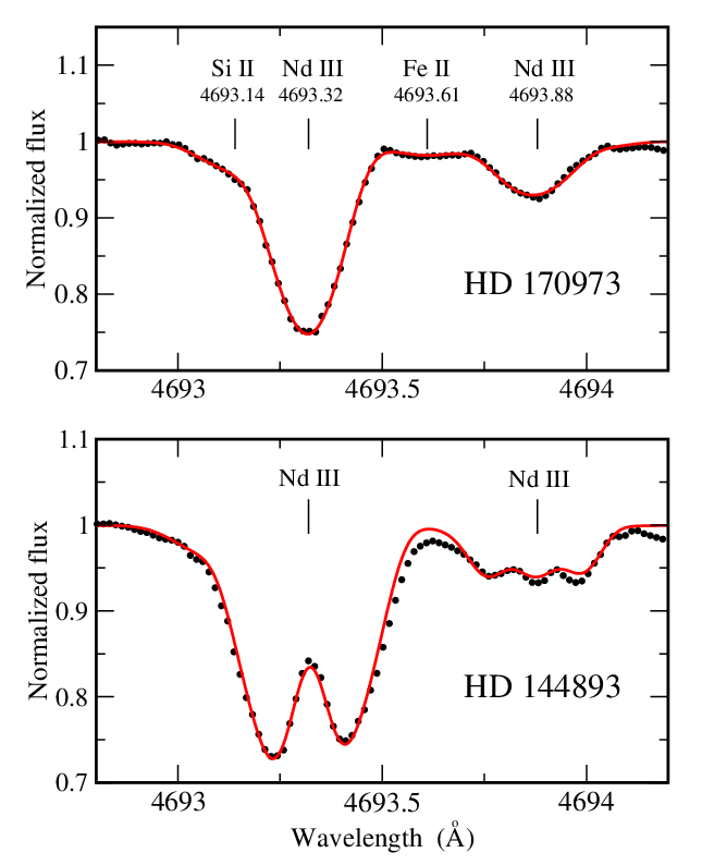
Figure 5: Observed (black dotted line) and synthesised (red line) spectra between 4692.5 - 4694.5 Å of HD 170973 and HD 144893 with surface magnetic fields $\langle B_{\rm z}\rangle$$<$1 kG and $\langle B_{\rm z}\rangle$=8.8 kG respectively, containing two newly classified transitions of Nd III: 4f^4 5F₅ - 4f³(⁴F)5d ⁵F₅ at 4693.32 Å and 4f^4 5G₅ - 4f³(⁴G)5d ⁵G₆ at 4693.88 Å.

The classification of transitions to 4f^4 5G₅ provided a useful guide on the expected relative intensities and SNRs of transitions from 4f³5d to other nearby low-lying 4f⁴ levels observed in the Nd-Ar PDL spectra. Subsequently, the 4f^4 3K_6,72 and 4f^4 5F₅ levels were confidently identified with support from H. M. Crosswhite’s unclassified list of 643 Nd III lines. Most notably, these lines from her sliding spark grating spectra indicated several transitions that were weak, blended, and/or not fitted in the Nd-Ar PDL spectra. The 4 levels belonging to 3 separate terms of the 4f⁴ configuration improved our Cowan code parameterisation, and the identifications of 4f^4 3K₈2, 4f^4 5G_3,4, and 4f^4 3H₅4 followed with confirmations from stellar spectra, which also enabled the identification of more levels of the 4f³(⁴F)5d, 4f³(²H2)5d, 4f³(⁴G)5d and 4f³(⁴D)5d (assigned) sub-configurations.

Identification of the 4f^4 5F_2,3,4 levels proved more challenging. The transitions 4f^4 5F_J - 4f³(⁴S)5d ⁵D_J-1 ($J>1$) were tentatively classified prior to the establishment of their energy levels, using their high intensities, isotope profiles, agreement in intensity and wavenumber with calculations, and presence in H. M. Crosswhite’s unclassified Nd III line list and the stars. But the 4f^4 5F_J - 4f³(⁴S)5d ⁵D_J transitions were expected around the noise level with too many candidate classifications, so the levels of 4f^4 5F and 4f³(⁴S)5d ⁵D terms could not be established using only the transitions between them. In looking for other evidence to resolve these ambiguities, the 4f³(⁴F)6p ⁵G_2,3,4,5 levels proved useful, which were identified using the VS grating spectra with the strongest lines to 4f³(⁴F)5d ⁵H_3,4,5,6 also observed in the PDL spectrum respectively (the same applied in the identifications of the 4f³(²H2)6p levels). The 4f³(⁴F)6p ⁵G levels aided the identification of the 4f³(⁴F)5d ⁵F_2,3,4 levels, which had transitions to 4f^4 5F_2,3,4 at intermediate SNRs. Even when additionally considering transitions from 4f³(⁴F)5d ⁵F_2,3,4, several attempts were made at classifying the 4f^4 5F_2,3,4 - 4f³5d transitions in the Nd-Ar PDL spectra before an agreement could be reached with lines observed in the stellar spectra.

6 Outlook

This extended analysis of the four low-lying configurations 4f⁴, 4f³5d, 4f³6s, and 4f³6p of Nd III will enable laboratory measurements of their lifetime and branching fractions for accurate transition probabilities. The experimentally established energy levels will improve future atomic structure calculations of Nd III by serving as benchmarks and semi-empirical constraints.

Attempts to identify levels of the doubly-excited configurations of Nd III were unsuccessful, the strongest predicted transitions originating from 4f²5d² are to the still unknown levels of the 4f³5d configuration. The remaining unknown 4f⁴ - 4f³5d transitions are expected to be very weak in the recorded Nd-Ar PDL FT spectra, with too many ambiguities in the expected intensity patterns and wavenumber ranges. Further large-scale experimental investigations of Nd III atomic structure would require extensions of the presented experimental and analysis methods, e.g., altering Nd discharge conditions to better populate higher-lying Nd III energy levels and to separate Nd III lines from other species, and/or establishing isolated energy level systems with strong lines which would eventually be connected to the current network of levels to the ground level.

Energy levels of the 4f³(⁴I)6d and 4f³(⁴I)7s sub-configurations have been identified in the Nd-Ar PDL FT spectra together with aid from the Nd VS grating spectra, they lie about 6000 cm^-1 lower than predicted by Gaigalas et al. (2019). Levels of the 4f³5f configuration are also being established from the classification of the 4f³5d - 4f³5f transitions in another set of Nd grating spectra recorded in the range 820-1159 Å. These results, totaling more than 100 energy levels, are being prepared for publication, where the energy level and transition probability calculations by Cowan’s codes will also be included in full.

Many energy levels of Nd I-III remain unknown experimentally, as more than $10^{4}$ lines are still unclassified in the Nd-Ar PDL spectra. The Penning discharge lamp design has shown to be a suitable source of Nd spectra, with particular enhancements of Nd II and Nd III populations compared to the alternative HCL at running conditions which maximised the Nd III resonance line intensities. For further investigations of Nd and other lanthanide elements, high-resolution spectroscopy of varying plasma conditions, accurate semi-empirical atomic structure calculations, and rigorous line list extraction methods are emphasised to be key strategies.

7 Summary

144 energy levels of Nd III have been determined from the classification of 433 Nd III transitions measured by Fourier transform spectroscopy of Nd Penning lamp discharges between 11500-54000 cm^-1 (8695-1852 Å) supplemented by grating spectroscopy of Nd vacuum sliding sparks and Nd-rich stars. 39 previously published energy levels were confirmed and 105 new levels of the 4f⁴, 4f³5d, 4f³6s, and 4f³6p configurations are reported here for the first time. These results are the most extensive and most accurate (to a few 10^-3 cm^-1) Nd III energy level and transition wavenumber data to date, which will enable the wider and more reliable application of Nd III atomic data in astronomy.

References

- Abbott et al. (2017) Abbott, B. P., Abbott, R., Abbott, T., et al. 2017, Phys. Rev. Lett., 119, 161101
- Aldenius (2001) Aldenius, M. 2001, Master’s thesis, University of Lund
- Azarov (1991) Azarov, V. 1991, Preprint of the Institute of Spectroscopy, Russian Academy of Sciences, Troitsk, 1, doi: 10.5281/zenodo.8108975
- Azarov et al. (2018) Azarov, V., Kramida, A., & Vokhmentsev, M. Y. 2018, CoPhC, 225, 149
- Berglund & Wieser (2011) Berglund, M., & Wieser, M. E. 2011, PApCh, 83, 397
- Blaise et al. (1984) Blaise, J., Wyart, J.-F., Djerad, M. T., & Ahmed, Z. B. 1984, PhyS, 29, 119
- Blaise et al. (1971) Blaise, J., Wyart, J.-F., Hoekstra, R., & Kruiver, P. 1971, JOSA, 61, 1335
- Bord (2000) Bord, D. 2000, A&AS, 144, 517
- Brewer (1971) Brewer, L. 1971, JOSA, 61, 1666
- Clear et al. (2022) Clear, C. P., Pickering, J. C., Nave, G., Uylings, P., & Raassen, T. 2022, ApJS, 261, 35
- Coulter et al. (2017) Coulter, D., Foley, R., Kilpatrick, C., et al. 2017, Sci, 358, 1556
- Cowan (1981) Cowan, R. D. 1981, The theory of atomic structure and spectra (Univ of California Press)
- Cowley et al. (2000) Cowley, C. R., Ryabchikova, T., Kupka, F., et al. 2000, MNRAS, 317, 299
- Davis et al. (2001) Davis, S. P., Abrams, M. C., & Brault, J. W. 2001, Fourier transform spectrometry (Elsevier)
- Dieke et al. (1961) Dieke, G., Crosswhite, H., & Dunn, B. 1961, JOSA, 51, 820
- Dieke & Crosswhite (1963) Dieke, G. H., & Crosswhite, H. 1963, Appl. Opt., 2, 675
- Dzuba et al. (2003) Dzuba, V., Safronova, U., & Johnson, W. 2003, Phys. Rev. A, 68, 032503
- Engström (1998) Engström, L. 1998, Lund Rep Atom Phys, LRAP
- Finley et al. (1979) Finley, D. S., Bowyer, S., Paresce, F., & Malina, R. F. 1979, Appl. Opt., 18, 649
- Fontes et al. (2020) Fontes, C., Fryer, C., Hungerford, A., Wollaeger, R., & Korobkin, O. 2020, MNRAS, 493, 4143
- Gaigalas et al. (2019) Gaigalas, G., Kato, D., Rynkun, P., Radžiūtė, L., & Tanaka, M. 2019, ApJS, 240, 29
- Gillanders et al. (2021) Gillanders, J. H., McCann, M., Sim, S., Smartt, S., & Ballance, C. P. 2021, MNRAS, 506, 3560
- Haris & Kramida (2017) Haris, K., & Kramida, A. 2017, ApJS, 233, 16
- Heise et al. (1994) Heise, C., Hollandt, J., Kling, R., Kock, M., & Kühne, M. 1994, Appl. Opt., 33, 5111
- Johnson & Nelson (2017) Johnson, D. A., & Nelson, P. G. 2017, JPCRD, 46, 013109
- Kasen et al. (2013) Kasen, D., Badnell, N., & Barnes, J. 2013, ApJ, 774, 25
- Kato (2003) Kato, K.-I. 2003, PASJ, 55, 1133
- Koczorowski et al. (2005) Koczorowski, W., Stachowska, E., Furmann, B., et al. 2005, AcSpA, 60, 447
- Kramida (2011) Kramida, A. 2011, CoPhC, 182, 419
- Kramida (2021) —. 2021, National Institute of Standards and Technology: Gaithersburg, MD, USA, doi: 10.18434/T4/1502500
- Kramida et al. (2022) Kramida, A., Ralchenko, Y., Reader, J., & the NIST ASD Team. 2022, NIST Atomic Spectra Database (version 5.10), National Institute of Standards and Technology, Gaithersburg, MD, doi: 10.18434/T4W30F
- Lawler et al. (2022) Lawler, J., Schmidt, J., & Den Hartog, E. 2022, J. Quant. Spec. Radiat. Transf., 289, 108283
- Learner & Thorne (1988) Learner, R., & Thorne, A. 1988, JOSAB, 5, 2045
- Liggins et al. (2021) Liggins, F. S., Pickering, J. C., Nave, G., Ward, J. W., & Tchang-Brillet, W.-Ü. L. 2021, ApJS, 252, 10
- Lodders (2021) Lodders, K. 2021, Space Sci. Rev., 217, 44
- Martin et al. (1978) Martin, W. C., Zalubas, R., & Hagan, L. 1978, Atomic Energy Levels - The Rare-Earth Elements (U.S.: Nat. Bur. Stand.), 422, doi: 10.6028/NBS.NSRDS.60
- Mashonkina et al. (2009) Mashonkina, L., Ryabchikova, T., Ryabtsev, A., & Kildiyarova, R. 2009, Astronomy & Astrophysics, 495, 297
- Meftah et al. (2008) Meftah, A., Wyart, J.-F., Sinzelle, J., et al. 2008, Physica Scripta, 77, 055302
- Nave et al. (2015) Nave, G., Griesmann, U., Brault, J., & Abrams, M. 2015, ascl soft, ascl:1511.004
- Palmeri et al. (2000) Palmeri, P., Quinet, P., Frémat, Y., Wyart, J.-F., & Biémont, E. 2000, The Astrophysical Journal Supplement Series, 129, 367
- Peck & Reeder (1972) Peck, E. R., & Reeder, K. 1972, JOSA, 62, 958
- Przybylski (1977) Przybylski, A. 1977, MNRAS, 178, 71
- Radziemski & Andrew (1965) Radziemski, L. J., & Andrew, K. L. 1965, JOSA, 55, 474
- Ryabchikova et al. (2008) Ryabchikova, T., Kochukhov, O., & Bagnulo, S. 2008, A&A, 480, 811
- Ryabchikova et al. (2011) Ryabchikova, T., LeBlanc, F., & Shulyak, D. 2011, in Magnetic Stars, 69–80
- Ryabchikova et al. (2006) Ryabchikova, T., Ryabtsev, A., Kochukhov, O., & Bagnulo, S. 2006, A&A, 456, 329
- Saloman (2010) Saloman, E. B. 2010, JPCRD, 39, 033101
- Silva et al. (2022) Silva, R. F., Sampaio, J. M., Amaro, P., et al. 2022, Atoms, 10, 18
- Smartt et al. (2017) Smartt, S., Chen, T.-W., Jerkstrand, A., et al. 2017, Nature, 551, 75
- Stancik & Brauns (2008) Stancik, A. L., & Brauns, E. B. 2008, Vib. Spectrosc., 47, 66
- Tanaka & Hotokezaka (2013) Tanaka, M., & Hotokezaka, K. 2013, ApJ, 775, 113
- Tanaka et al. (2020) Tanaka, M., Kato, D., Gaigalas, G., & Kawaguchi, K. 2020, MNRAS, 496, 1369
- Tanaka et al. (2018) Tanaka, M., Kato, D., Gaigalas, G., et al. 2018, ApJ, 852, 109
- Thorne et al. (1987) Thorne, A., Harris, C., Wynne-Jones, I., Learner, R., & Cox, G. 1987, JPhE, 20, 54
- Valenti et al. (2017) Valenti, S., David, J., Yang, S., et al. 2017, ApJ, 848, L24
- Watson et al. (2019) Watson, D., Hansen, C. J., Selsing, J., et al. 2019, Nature, 574, 497
- Whaling et al. (1995) Whaling, W., Anderson, W., Carle, M., Brault, J., & Zarem, H. 1995, J. Quant. Spec. Radiat. Transf., 53, 1
- Whaling et al. (2002) —. 2002, NISTJ, 107, 149
- Wyart (2010) Wyart, J.-F. 2010, PhyS, 82, 035302
- Wyart et al. (2007) Wyart, J.-F., Meftah, A., Tchang-Brillet, W.-Ü. L., et al. 2007, JPhB, 40, 3957
- Wyart et al. (2010) Wyart, J.-F., Tchang Brillet, W.-U., Ryabtsev, A. N., et al. 2010, Book of abstracts, 7th International Conference on Atomic and Molecular Data and their Applications, Vilnius.
- Zhang et al. (2002) Zhang, Z., Svanberg, S., Palmeri, P., Quinet, P., & Biémont, E. 2002, A&A, 385, 724