Noncompact uniform universal approximation

Abstract

The universal approximation theorem is generalised to uniform convergence on the (noncompact) input space $\mathbb{R}^{n}$. All continuous functions that vanish at infinity can be uniformly approximated by neural networks with one hidden layer, for all activation functions $\varphi$ that are continuous, nonlinear, and asymptotically linear at $\pm\infty$. When $\varphi$ is moreover bounded, we exactly determine which functions can be uniformly approximated by neural networks, with the following unexpected results. Let $\overline{\mathcal{N}_{\varphi}^{l}(\mathbb{R}^{n})}$ denote the vector space of functions that are uniformly approximable by neural networks with $l$ hidden layers and $n$ inputs. For all $n$ and all $l\geq 2$, $\overline{\mathcal{N}_{\varphi}^{l}(\mathbb{R}^{n})}$ turns out to be an algebra under the pointwise product. If the left limit of $\varphi$ differs from its right limit (for instance, when $\varphi$ is sigmoidal) the algebra $\overline{\mathcal{N}_{\varphi}^{l}(\mathbb{R}^{n})}$ ($l\geq 2$) is independent of $\varphi$ and $l$, and equals the closed span of products of sigmoids composed with one-dimensional projections. If the left limit of $\varphi$ equals its right limit, $\overline{\mathcal{N}_{\varphi}^{l}(\mathbb{R}^{n})}$ ($l\geq 1$) equals the (real part of the) commutative resolvent algebra, a C*-algebra which is used in mathematical approaches to quantum theory. In the latter case, the algebra is independent of $l\geq 1$, whereas in the former case $\overline{\mathcal{N}_{\varphi}^{2}(\mathbb{R}^{n})}$ is strictly bigger than $\overline{\mathcal{N}_{\varphi}^{1}(\mathbb{R}^{n})}$.

1 Introduction

Neural networks can uniformly approximate any continuous function only when the size of the input values is bounded by a predetermined constant. Typical universal approximation theorems that use the entire noncompact input space $\mathbb{R}^{n}$ make use of convergence ‘uniformly on compacts’ [1, 5, 6, 8, 9, 11, 13] or convergence with respect to an integral norm on $\mathbb{R}^{n}$ [8, 10]. Such theorems do not rule out errors in the approximation growing exponentially (or worse) in the size of the input values.

Noncompact and uniform approximation – which uses convergence with respect to the supremum norm over $\mathbb{R}^{n}$ – is a much stronger notion. In theory, it allows one to train a network up to a desired precision which is then respected by all input values. It also gives a more honest picture of the generalization capability of neural networks, as we shall see later.

It is a common misconception that every continuous function on $\mathbb{R}^{n}$ can be uniformly approximated; in fact many commonplace continuous functions cannot. The question remains: precisely which functions can be uniformly approximated?

Let the activation function $\varphi\mathrel{\mathop{\mathchar 58\relax}}\mathbb{R}\to\mathbb{R}$ be continuous and nonlinear, with asymptotically linear behaviour near $\pm\infty$. One-layer neural networks are by definition linear combinations of functions of the form

$$x\mapsto\varphi(a\cdot x+b)\qquad(a\in\mathbb{R}^{n},b\in\mathbb{R}),$$ (1)

where $\cdot$ is the standard inner product on $\mathbb{R}^{n}$. Such functions are constant in $n-1$ directions. If $n\geq 2$, a nonzero one-layer neural network will therefore never be in $C_{0}(\mathbb{R}^{n})$, the space of continuous functions that vanish at infinity, no matter the activation function or the amount of nodes. Our first result is that, nonetheless, all functions in $C_{0}(\mathbb{R}^{n})$ are uniformly approximable by one-layer neural networks (and therefore also by arbitrarily deep neural networks). This generalizes the universal approximation theorem to a truely noncompact statement.

We also precisely characterise the space of (uniformly) approximable functions in the case that $\varphi$ is moreover bounded. The above result already implies that the space of approximable functions is some vector space between $C_{0}(\mathbb{R}^{n})$ and the space of bounded continuous functions, $C_{\textnormal{b}}(\mathbb{R}^{n})$.

By giving an explicit characterisation, we shall prove that this vector space is an algebra under the usual pointwise operations. Equivalently, products of neural networks are approximable by neural networks.

This uncovers a novel connection between neural networks and the theory of C*-algebras [16], as any norm-closed subalgebra of $C_{\textnormal{b}}(\mathbb{R}^{n})$ is a real C*-algebra. We do not rely on the theory of C*-algebras in this paper, but one should know that this theory initiated these findings, and might have merit for the machine learning community for reasons discussed in [7].

Below, we discuss the explicit characterisation of the space of approximable functions, which notably does not depend greatly on the activation function $\varphi$, but only on the question whether $\varphi(-\infty)\mathrel{\mathop{\mathchar 58\relax}}=\lim_{x\to-\infty}\varphi(x)$ equals $\varphi(\infty)\mathrel{\mathop{\mathchar 58\relax}}=\lim_{x\to\infty}\varphi(x)$.

1.1 The case $\varphi(-\infty)=\varphi(\infty)$

We first consider the class of $\varphi$ satisfying $\varphi(-\infty)=\varphi(\infty)$. We find that, for any amount of hidden layers, the vector space of approximable functions is equal to the real part of the commutative resolvent algebra, defined in [17]. This is a space of bounded functions built up from copies of $C_{0}(V)$ on linear subspaces $V$ of $\mathbb{R}^{n}$.

In [2, 17, 18, 20], the commutative resolvent algebra is studied because it is the classical counterpart of the resolvent algebra, a quantum observable algebra that was introduced in [3, 4] for the purpose of (nonrelativistic) algebraic quantum field theory. This establishes a connection between machine learning and quantum algebra that seems unexplored so far, and for instance different from standard approaches to quantum neural networks [22]. A useful application of the noncompact uniform approximation theorem to mathematical quantum physics will be demonstrated in a separate paper [19].

1.2 The case $\varphi(-\infty)\neq\varphi(\infty)$

Our final main theorem expresses the space of approximable functions in the case of $\varphi(-\infty)\neq\varphi(\infty)$ and gives novel insight into the approximation capability and limitations of neural networks.

When using two or more hidden layers, the space of approximable functions equals the closed span of products of sigmoids composed with one-dimensional projections. A way to visualize these products is as the wedge-shaped functions appearing in Figure 2 and Definition 5.21, related to Voronoi diagrams [15] and tropical geometry [14, 23], and familiar to anyone who has ever visualised the approximation behavior of neural networks in cases were there is a sufficiently complicated structure in the data. Indeed, when a neural network is prioritizing the fitting of a small-scale structure, at a slightly larger scale one can often see the wedge functions of Definition 5.21 appearing. See, for example, Figure 1. In fact, the rigidity of these wedge functions can prevent the neural network from converging locally if there are not enough nodes or there is not enough time. Thus the proof in Section 5 (although mathematically focussed on the ‘infinitely large scale’) offers a very satisfying explanation to the appearance of such wedge shapes (whether features or artefacts) in practical applications.

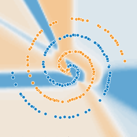
Figure 1: Example of a neural network in which wedge functions (cf. Definition 5.21 and Figure 2) are clearly visible in the contour plot. The network has been given insufficient nodes/layers/time to fit the data at all relevant scales, and has only succeeded on the small scale. At a slightly larger scale the wedge functions already become apparent, and this paper proves that this behaviour is in fact unavoidable at sufficiently large scale. This image was produced using matlabsolutions.com/visualize-neural-network/neural-network.html.

Opposite to the earlier case, in the present case ($\varphi(-\infty)\neq\varphi(\infty)$) there are two-layer neural networks which cannot be approximated by one-layer neural networks. We shall give a class of examples of such functions, some of which being quite simple.

2 Notation and summary of main results

We let $\mathbb{N}=\{1,2,\ldots\}$. We work over the field $\mathbb{R}$. For any $n\in\mathbb{N}$, we denote by $C(\mathbb{R}^{n})$, $C_{\textnormal{b}}(\mathbb{R}^{n})$, $C_{0}(\mathbb{R}^{n})$, and $C_{\textnormal{c}}(\mathbb{R}^{n})$ respectively the continuous functions from $\mathbb{R}^{n}$ to $\mathbb{R}$, the bounded ones, the ones vanishing at infinity (i.e., $\lim_{\|x\|\to\infty}f(x)=0$), and the compactly supported ones. The support of a function $f$ is denoted $\operatorname{supp}f$. By $\overline{S}$ we denote the uniform closure of a set $S$ of functions $\mathbb{R}^{n}\to\mathbb{R}$, i.e., the closure in the topology induced by the extended metric obtained from the supremum norm. We denote $\overline{\textnormal{span}}\,S\mathrel{\mathop{\mathchar 58\relax}}=\overline{\textnormal{span}\,S}$, where $\textnormal{span}\,S$ is the $\mathbb{R}$-linear span of $S$. For $a,x\in\mathbb{R}^{n}$, we denote by $a\cdot x\mathrel{\mathop{\mathchar 58\relax}}=\sum_{j=1}^{n}a_{j}x_{j}$ the Euclidean inner product, and define functions $p_{a}\mathrel{\mathop{\mathchar 58\relax}}\mathbb{R}^{n}\to\mathbb{R}$ by $p_{a}(x)\mathrel{\mathop{\mathchar 58\relax}}=a\cdot x$. We let $P_{V}\mathrel{\mathop{\mathchar 58\relax}}\mathbb{R}^{n}\to V$ denote the orthogonal projection onto any linear subspace $V\subseteq\mathbb{R}^{n}$.

Let $\varphi\mathrel{\mathop{\mathchar 58\relax}}\mathbb{R}\to\mathbb{R}$ be a function. We define the space of neural networks with $n$ input nodes, one hidden layer, one output node, and activation function $\varphi$, as the following subspace of the vector space of all functions $\mathbb{R}^{n}\to\mathbb{R}$:

$$\mathcal{N}_{\varphi}^{1}(\mathbb{R}^{n})\mathrel{\mathop{\mathchar 58\relax}}=\textnormal{span}\,\Big{\{}x\mapsto\varphi(a\cdot x+b)\leavevmode\nobreak\ \Big{|}\leavevmode\nobreak\ a\in\mathbb{R}^{n},\leavevmode\nobreak\ b\in\mathbb{R}\Big{\}}.$$ (2)

The space of networks with $l$ hidden layers can then be defined recursively:

$$\mathcal{N}_{\varphi}^{l}(\mathbb{R}^{n})\mathrel{\mathop{\mathchar 58\relax}}=\textnormal{span}\left\{x\mapsto\varphi(f(x)+b)\leavevmode\nobreak\ \middle|\leavevmode\nobreak\ f\in\mathcal{N}_{\varphi}^{l-1}(\mathbb{R}^{n}),\leavevmode\nobreak\ b\in\mathbb{R}\right\}.$$

The space of networks with an arbitrary amount of hidden layers is denoted by $\mathcal{N}_{\varphi}^{\leavevmode\nobreak\ }(\mathbb{R}^{n})\mathrel{\mathop{\mathchar 58\relax}}=\bigcup_{l=1}^{\infty}\mathcal{N}_{\varphi}^{l}(\mathbb{R}^{n}).$ Most results shall be stated for networks with only one output node, because extending these results to $m$ output nodes, i.e., to the spaces $\mathcal{N}_{\varphi}^{l}(\mathbb{R}^{n},\mathbb{R}^{m})\mathrel{\mathop{\mathchar 58\relax}}=\mathcal{N}_{\varphi}^{l}(\mathbb{R}^{n})^{\oplus m}$ and $\mathcal{N}_{\varphi}^{\leavevmode\nobreak\ }(\mathbb{R}^{n},\mathbb{R}^{m})\mathrel{\mathop{\mathchar 58\relax}}=\cup_{l}\mathcal{N}_{\varphi}^{l}(\mathbb{R}^{n},\mathbb{R}^{m})$, is straightforward.

The following theorem summarizes our first main result, which is formulated for the largest possible class of activation functions in Theorem 3.11.

Theorem 2.1.

Let $n,l\in\mathbb{N}$, and let $\varphi\in C(\mathbb{R})$ be nonlinear with $\lim_{x\to\infty}(\varphi(x)-a_{1}x-b_{1})=0$ and $\lim_{x\to-\infty}(\varphi(x)-a_{2}x-b_{2})=0$ for $a_{1},b_{1},a_{2},b_{2}\in\mathbb{R}$. Then,

$$C_{0}(\mathbb{R}^{n})\subseteq\overline{\mathcal{N}_{\varphi}^{l}(\mathbb{R}^{n})}.$$

The following theorem summarizes our second and third main result, which are written in stronger form as Theorem 4.15 and Theorem 5.23.

Theorem 2.2.

Let $n\in\mathbb{N}$, and let $\varphi\in C(\mathbb{R})$ be nonconstant such that $\varphi(-\infty)=\lim_{x\to-\infty}\varphi(x)$ and $\varphi(\infty)=\lim_{x\to\infty}\varphi(x)$ exist and are finite.

1. If $\varphi(-\infty)=\varphi(\infty)$ then $\overline{\mathcal{N}_{\varphi}^{1}(\mathbb{R}^{n})}=\overline{\mathcal{N}_{\varphi}^{\leavevmode\nobreak\ }(\mathbb{R}^{n})}$ and

   $$\overline{\mathcal{N}_{\varphi}^{\leavevmode\nobreak\ }(\mathbb{R}^{n})}=\overline{\textnormal{span}}\left\{x\mapsto g(P(x))\leavevmode\nobreak\ \middle|\leavevmode\nobreak\ \begin{aligned} &P\mathrel{\mathop{\mathchar 58\relax}}\mathbb{R}^{n}\to\mathbb{R}^{k}\text{ linear surjection,}\\ &g\in C_{0}(\mathbb{R}^{k}),\leavevmode\nobreak\ k\in\mathbb{N}\end{aligned}\right\}.$$

2. If $\varphi(-\infty)\neq\varphi(\infty)$ then $\overline{\mathcal{N}_{\varphi}^{1}(\mathbb{R}^{n})}\neq\overline{\mathcal{N}_{\varphi}^{2}(\mathbb{R}^{n})}=\overline{\mathcal{N}_{\varphi}^{\leavevmode\nobreak\ }(\mathbb{R}^{n})}$ and

   $$\overline{\mathcal{N}_{\varphi}^{\leavevmode\nobreak\ }(\mathbb{R}^{n})}=\overline{\textnormal{span}}\,\Bigg{\{}x\mapsto\prod_{j=1}^{m}\tanh(a_{j}\cdot x)\leavevmode\nobreak\ \Bigg{|}\leavevmode\nobreak\ m\in\mathbb{N},a_{1},\ldots,a_{m}\in\mathbb{R}^{n}\Bigg{\}}.$$

The sigmoid $\tanh$ is used for explicitness, but can be replaced by any sigmoid of choice, as will be discussed in Section 5.

Corollary 2.3.

Let $n,m\in\mathbb{N}$ and let $\varphi\in C(\mathbb{R})$ be such that $\lim_{x\to-\infty}\varphi(x)$ and $\lim_{x\to\infty}\varphi(x)$ exist and are finite. Then the vector space $\overline{\mathcal{N}_{\varphi}^{\leavevmode\nobreak\ }(\mathbb{R}^{n},\mathbb{R}^{m})}$ is an algebra. Equivalently, pointwise products of neural networks are uniformly approximable by neural networks.

Proof.

For $\varphi=0$, we have $\overline{\mathcal{N}_{\varphi}^{\leavevmode\nobreak\ }(\mathbb{R}^{n},\mathbb{R}^{m})}=\{0\}$ so the statement is trivial. Otherwise, the corollary follows from Theorem 2.2, by applying [17, Lemma 2.2] in the case of $\varphi(-\infty)=\varphi(\infty)$. ∎

A particular aspect of Theorem 2.2 is that, for $\varphi(-\infty)\neq\varphi(\infty)$, there exist functions in $\overline{\mathcal{N}_{\varphi}^{2}(\mathbb{R}^{n})}$ that are not in $\overline{\mathcal{N}_{\varphi}^{1}(\mathbb{R}^{n})}$. In §5.2 we give a class of explicit examples (including a mollified AND function) and thus prove the following stronger statement.

Theorem 2.4.

Let $n\in\mathbb{N}$, and let $\varphi\in C(\mathbb{R})$ be such that $\lim_{x\to-\infty}\varphi(x)$ and $\lim_{x\to\infty}\varphi(x)$ exist and are finite and distinct. For every $d>0$, there are two-layer networks $f\in\mathcal{N}_{\varphi}^{2}(\mathbb{R}^{n})$ with a fixed distance $d$ from the whole collection of one-layer networks, $\mathcal{N}_{\varphi}^{1}(\mathbb{R}^{n})$.

That is, no matter how hard you train the one-layer network $g$ to approximate $f$, no matter the amount of nodes, there will exist an input value $x$ such that $|f(x)-g(x)|>d$.

3 Approximation of continuous functions vanishing at infinity

The purpose of this section is to prove Theorem 3.11, which states that $C_{0}(\mathbb{R}^{n})$ can be approximated by neural networks with one hidden layer. This result holds for a slightly larger class of activation functions than mentioned in Theorem 2.1, allowing discontinuities and polynomial increase.

However, we shall first prove this approximation theorem in the simpler case that $\varphi\in C_{0}(\mathbb{R})\setminus\{0\}$. Furthermore, it will be useful to first consider $n=1$ and $n=2$.

Lemma 3.5.

Let $\varphi\in C_{0}(\mathbb{R})\setminus\{0\}$. We have $\overline{\mathcal{N}^{1}_{\varphi}(\mathbb{R})}=C_{0}(\mathbb{R})\oplus\mathbb{R}1$.

Proof.

We observe that any function

$$x\mapsto\varphi(ax+b)\qquad(a,b\in\mathbb{R})$$

is in $C_{0}(\mathbb{R})$ when $a\neq 0$. If $a=0$, then the above map is constant, i.e., in $\mathbb{R}1$. We conclude that $\mathcal{N}^{1}_{\varphi}(\mathbb{R})\subseteq C_{0}(\mathbb{R})\oplus\mathbb{R}1$, and since $C_{0}(\mathbb{R})\oplus\mathbb{R}1$ is closed with respect to the supremum norm, we find that $\overline{\mathcal{N}^{1}_{\varphi}(\mathbb{R})}\subseteq C_{0}(\mathbb{R})\oplus\mathbb{R}1$

The rest of the proof proceeds exactly as in the proof of [5, Theorem 1], replacing $C([0,1]^{n})$ with $C_{0}(\mathbb{R})$ and replacing [5, Lemma 1] with [8, Theorem 5] (quite similar to the proof of Proposition 3.9). It is however good to note that this strategy naively fails for $C_{0}(\mathbb{R}^{n})$ when $n>1$, as the functions $x\mapsto\varphi(a\cdot x+b)$ are not in $C_{0}(\mathbb{R}^{n})$ when $n>1$. ∎

For $n>1$, a noncompact uniform approximation theorem requires new ideas not considered by, e.g., [5, 8, 10].

The core idea in the case $n=2$ is to give meaning to the formal expression

$$\int_{0}^{2\pi}g\circ p_{(\cos\theta,\sin\theta)}\,d\theta,$$ (3)

for a suitable function $g$ such that (3) is in $\overline{\mathcal{N}_{\varphi}^{1}(\mathbb{R}^{2})}$ and in a way generates $C_{0}(\mathbb{R}^{2})$. What complicates the proof is that, whatever (3) means, it is not a Bochner integral with respect to the supremum norm. Worse yet, the integrand both has inseparable range and is discontinuous, because $\|g\circ p_{(\cos\theta,\sin\theta)}-g\circ p_{(\cos\theta^{\prime},\sin\theta^{\prime})}\|\geq\|g\|_{\infty}$ for every $\theta\neq\theta^{\prime}\in[0,\pi)$. The following result shows that it nevertheless has an interpretation as an element of $\overline{\mathcal{N}_{\varphi}^{1}(\mathbb{R}^{2})}$.

Lemma 3.6.

Let $g\in C_{\textnormal{c}}(\mathbb{R})$ be Lipschitz continous. Define

$$f(x,y)\mathrel{\mathop{\mathchar 58\relax}}=\int_{0}^{2\pi}(g\circ p_{(\cos\theta,\sin\theta)})(x,y)\,d\theta$$ (4)

for all $(x,y)\in\mathbb{R}^{2}$ and

$$f_{N}\mathrel{\mathop{\mathchar 58\relax}}=\frac{2\pi}{N}\sum_{k=1}^{N}g\circ p_{(\cos\frac{2\pi k}{N},\sin\frac{2\pi k}{N})}\in\overline{\mathcal{N}_{\varphi}^{1}(\mathbb{R}^{2})}.$$

Then the sequence $(f_{2^{m}})_{m\geq 1}$ converges uniformly to $f$.

Proof.

For all $(x,y)\in\mathbb{R}^{2}$, we define the number

$$\Phi_{N}(x,y)\mathrel{\mathop{\mathchar 58\relax}}=\#\left\{k\in\{1,\ldots,N\}\leavevmode\nobreak\ \middle|\leavevmode\nobreak\ p_{(\cos\frac{2\pi k}{N},\sin\frac{2\pi k}{N})}(x,y)\in\operatorname{supp}g\right\},$$

which leads to the bound

$$|f_{N}(x,y)|\leq\frac{2\pi\left\|g\right\|_{\infty}}{N}\Phi_{N}(x,y).$$ (5)

If $R_{\theta}\mathrel{\mathop{\mathchar 58\relax}}\mathbb{R}^{2}\to\mathbb{R}^{2}$ denotes the rotation by an angle $\theta$, we have

$$\Phi_{N}(x,y)=\sum_{k=1}^{N}\Phi_{1}\big{(}R_{\frac{2\pi k}{N}}(x,y)\big{)}.$$ (6)

By using (6) twice, we obtain, for every $m,p\in\mathbb{N}$,

$$\Phi_{2^{m+p}}(x,y) =\sum_{j=1}^{2^{p}}\sum_{k=1}^{2^{m}}\Phi_{1}\big{(}R_{\frac{2\pi k}{2^{m}}}\big{(}R_{\frac{2\pi j}{2^{m+p}}}(x,y)\big{)}\big{)}$$

$$=\sum_{j=1}^{2^{p}}\Phi_{2^{m}}\big{(}R_{\frac{2\pi j}{2^{m+p}}}(x,y)\big{)}.$$ (7)

Moreover, for all $m\in\mathbb{N}$ there exists a closed disc $\overline{B_{r}(0)}$ around 0 with radius $r>0$ such that $\Phi_{2^{m}}(x,y)\leq 1$ for all $(x,y)$ outside this disc. Because discs around 0 are rotation invariant, it follows from (7) that $\Phi_{2^{m+p}}(x,y)\leq 2^{p}$ for all $p\in\mathbb{N}$ and $(x,y)$ outside $\overline{B_{r}(0)}.$ By (5), we conclude that for all $m\in\mathbb{N}$ there exists an $r>0$ such that

$$|f_{2^{m+p}}(x,y)|\leq\frac{2\pi\left\|g\right\|_{\infty}}{2^{m}}\qquad(p\in\mathbb{N},(x,y)\in\mathbb{R}^{2}\setminus\overline{B_{r}(0)}).$$ (8)

Restricting to $\overline{B_{r}(0)}$, the function

$$[0,2\pi)\to C_{\textnormal{b}}(\overline{B_{r}(0)}),\qquad\theta\mapsto(g\circ p_{(\cos\theta,\sin\theta)})\!\upharpoonright_{\overline{B_{r}(0)}}$$

is $\left\|\cdot\right\|_{\infty}$-continuous and separable valued, and hence Bochner integrable for all $r>0$. We define simple functions $s_{N}\mathrel{\mathop{\mathchar 58\relax}}[0,2\pi)\to C_{\textnormal{b}}(\overline{B_{r}(0)})$ by

$$s_{N}\mathrel{\mathop{\mathchar 58\relax}}=\sum_{k=1}^{N}(g\circ p_{(\cos\frac{2\pi k}{N},\sin\frac{2\pi k}{N})})\!\upharpoonright_{\overline{B_{r}(0)}}\,\cdot\,1_{\big{[}\frac{2\pi(k-1)}{N},\frac{2\pi k}{N}\big{)}},$$

where $1$ is the indicator function. We obtain $\int_{[0,2\pi)}s_{N}=f_{N}\!\upharpoonright_{\overline{B_{r}(0)}}$ and

$$\|s_{N}(\theta)-(g\circ p_{(\cos\theta,\sin\theta)})\!\upharpoonright_{\overline{B_{r}(0)}}\|_{\infty}\leq cr\Big{(}\big{|}\cos\tfrac{2\pi k_{N}}{N}-\cos\theta\big{|}$$

$$\quad+\big{|}\sin\tfrac{2\pi k_{N}}{N}-\sin\theta\big{|}\Big{)},$$

where $c$ is the Lipschitz constant of $g$ and $k_{N}$ is the unique number such that $\theta\in\big{[}\frac{2\pi(k_{N}-1)}{N},\frac{2\pi k_{N}}{N}\big{)}$. The above norm converges uniformly in $\theta$. Hence, elementary properties of the Bochner integral imply that

$$f\!\upharpoonright_{\overline{B_{r}(0)}}\leavevmode\nobreak\ =\int_{0}^{2\pi}(g\circ p_{(\cos\theta,\sin\theta)})\!\upharpoonright_{\overline{B_{r}(0)}}\,d\theta=\lim_{N\to\infty}f_{N}\!\upharpoonright_{\overline{B_{r}(0)}}$$

uniformly. Combining this with (8), we obtain the lemma. ∎

Lemma 3.7.

Let $g\in C_{\textnormal{c}}(\mathbb{R})$ satisfy

$$\int_{\mathbb{R}}g(x)\,dx=0,$$ (9)

and define $f$ as in (4). Then $f\in C_{0}(\mathbb{R}^{2})$. In fact, there exists $C\in\mathbb{R}$ such that

$$|f(x,y)|\leq\frac{C}{1+\|(x,y)\|^{3}}\qquad((x,y)\in\mathbb{R}^{2}).$$ (10)

Proof.

From a substitution in (4) it follows that

$$f(x,y)=\int_{-\pi}^{\pi}g(R\sin\theta)\,d\theta,$$

where $R=\sqrt{x^{2}+y^{2}}$. Let $a>0$ be such that $\operatorname{supp}g\subseteq[-a,a]$. If $R>0$ is large enough, the substitution $u=\sin\theta$ is valid, and we obtain

$$f(x,y)=\int_{-a/R}^{a/R}g(Ru)\frac{1}{\sqrt{1-u^{2}}}\,du$$

As $\frac{1}{\sqrt{1-u^{2}}}=1+\mathcal{O}(u^{2})$, there exists a $C>0$ such that, for large enough $R$, we have $|\frac{1}{\sqrt{1-u^{2}}}-1|\leq Cu^{2}$ for all $u\in[-a/R,a/R]$. As $\int g(Ru)du=0$, we obtain

$$|f(x,y)|\leq\int_{-a/R}^{a/R}|g(Ru)|Cu^{2}\,du=R^{-3}\int_{-a}^{a}|g(u)|Cu^{2}\,du,$$

which implies the lemma. ∎

The importance of the following lemma can be appreciated by noting that, for all $f\in\mathcal{N}_{\varphi}^{1}(\mathbb{R}^{2})$, the corresponding $\psi$ is either constant or undefined.

Lemma 3.8.

Let $\varphi\in C_{0}(\mathbb{R})$, and let $g\in C_{\textnormal{c}}(\mathbb{R})$ be Lipschitz continuous and satisfy $\int g(x)=0$ and $\int g(x)x^{2}\neq 0$. Let $f$ be defined by (4). Then $f\in C_{0}(\mathbb{R}^{2})\cap\overline{\mathcal{N}_{\varphi}^{1}(\mathbb{R}^{2})}$ is $\mathcal{O}(-3)$. Furthermore, the integral

$$\psi(x)=\int_{\mathbb{R}}f(x,y)\,dy$$

defines a function $\psi\in L^{1}(\mathbb{R})\cap C_{0}(\mathbb{R})$. Lastly, $\psi$ is nonzero.

Proof.

All statements except the last follow directly from Lemmas 3.6 and 3.7. For the last statement, we note that the proof of Lemma 3.7 can be sharpened by using $\frac{1}{\sqrt{1-u^{2}}}=1+\tfrac{1}{2}u^{2}+\mathcal{O}(u^{4})$. Again denoting $R=\sqrt{x^{2}+y^{2}}$, we obtain

$$f(x,y)=R^{-3}\int_{-a}^{a}g(u)\tfrac{1}{2}u^{2}\,du+\mathcal{O}(R^{-5}).$$

Without loss of generality, $\int g(u)u^{2}>0$. We have $R\geq|x|$, so if $x$ is large enough, $f(x,y)>0$ for all $y\in\mathbb{R}$. Hence $\psi(x)>0$ for such $x$. ∎

Proposition 3.9.

For all $\varphi\in C_{0}(\mathbb{R})$ we have $C_{0}(\mathbb{R}^{2})\subseteq\overline{\mathcal{N}_{\varphi}^{1}(\mathbb{R}^{2})}$.

Proof.

With the intention of finding a contradiction, we assume that $\overline{\mathcal{N}_{\varphi}^{1}(\mathbb{R}^{2})}\cap C_{0}(\mathbb{R}^{2})\neq C_{0}(\mathbb{R}^{2})$. By the Hahn–Banach theorem, we obtain a continuous linear map $L\mathrel{\mathop{\mathchar 58\relax}}C_{0}(\mathbb{R}^{2})\to\mathbb{R}$ such that $L\left(\overline{\mathcal{N}_{\varphi}^{1}(\mathbb{R}^{2})}\cap C_{0}(\mathbb{R}^{2})\right)=\{0\}$ and $L\neq 0$. By the Riesz–Markov–Kakutani theorem, there exists a finite signed measure $\mu$ such that

$$L(f)=\int_{\mathbb{R}^{2}}f(x,y)d\mu(x,y)\qquad(f\in C_{0}(\mathbb{R}^{2})).$$

As $L\neq 0$, we obtain $\mu\neq 0$. Let $g,f,\psi$ be as in Lemma 3.8.

For all $a\in\mathbb{R}^{2}$ and $b,y\in\mathbb{R}$, let $a_{\perp}\in\mathbb{R}^{2}$ be any vector such that $a\cdot a_{\perp}=0$. Define $\tilde{f}_{a,a_{\perp},b,y}(v)\mathrel{\mathop{\mathchar 58\relax}}=f(a\cdot v+b,a_{\perp}\cdot v+y)$ for $v\in\mathbb{R}^{2}$. By translation invariance, $\tilde{f}_{a,a_{\perp},b,y}\in\overline{\mathcal{N}_{\varphi}^{1}(\mathbb{R}^{2})}\cap C_{0}(\mathbb{R}^{2})$. By a substitution, and (10), we find

$$\int_{\mathbb{R}^{2}}\psi(a\cdot v+b)\,d\mu(v) =\int_{\mathbb{R}^{2}}\int_{\mathbb{R}}f(a\cdot v+b,y)\,dy\,d\mu(v)$$

$$=\int_{\mathbb{R}}\int_{\mathbb{R}^{2}}f(a\cdot v+b,a_{\perp}\cdot v+y)\,d\mu(v)\,dy$$

$$=\int_{\mathbb{R}}L(\tilde{f}_{a,a_{\perp},b,y})\,dy=0.$$ (11)

But, since $\psi$ is bounded and nonconstant, [8, Theorem 5] implies that there exists no nonzero finite measure $\mu$ such that (3) holds. We obtain a contradiction, which implies the lemma. ∎

We now move to higher dimensions, and obtain a noncompact uniform approximation theorem in the case that $\varphi\in C_{0}(\mathbb{R})\setminus\{0\}$.

Proposition 3.10.

Let $\varphi\in C_{0}(\mathbb{R})\setminus\{0\}$, and let $n\in\mathbb{N}$. Any function in $C_{0}(\mathbb{R}^{n})$ is uniformly approximable on $\mathbb{R}^{n}$ by functions of the form

$$x\mapsto\sum_{j=1}^{k}c_{j}\,\varphi(a_{j}\cdot x+b_{j}),$$

for $k\in\mathbb{N}$, $b_{j},c_{j}\in\mathbb{R}$, and $a_{j}\in\mathbb{R}^{n}$. In fact, for any $l\in\mathbb{N}$,

$$C_{0}(\mathbb{R}^{n})\subseteq\overline{\mathcal{N}_{\varphi}^{l}(\mathbb{R}^{n})}.$$

Proof.

We use induction to $n$, and notice that $n=1$ is Lemma 3.5 and $n=2$ is Proposition 3.9. For $n>2$, we use $C_{0}(\mathbb{R}^{n})=\overline{C_{0}(\mathbb{R})\otimes C_{0}(\mathbb{R}^{n-1})}$, so in order to prove the first statement of the proposition it suffices to show that any function

$$(x_{1},\ldots,x_{n})\mapsto f_{1}(x_{1})f_{2}(x_{2},\ldots,x_{n})$$

can be uniformly approximated by one-layer networks, for $f_{1}\in C_{0}(\mathbb{R})$ and $f_{2}\in C_{0}(\mathbb{R}^{n-1})$. By induction hypothesis, $f_{2}$ can be uniformly approximated by linear combinations of $\varphi\circ p_{a}$ ($a\in\mathbb{R}^{n-1}$), so we may assume without loss of generality that $f_{2}=\varphi\circ p_{a}$ for $a\in\mathbb{R}^{n-1}$. It then suffices to approximate the function

$$(x_{1},\ldots,x_{n})\mapsto f_{1}(x_{1})(\varphi\circ p_{a})(x_{2},\ldots,x_{n}),$$

which equals $(f_{1}\otimes\varphi)\circ P$ for the linear surjection $P\mathrel{\mathop{\mathchar 58\relax}}\mathbb{R}^{n}\to\mathbb{R}^{2}$ given by $P(x_{1},\ldots,x_{n})=(x_{1},p_{a}(x_{2},\ldots,x_{n}))$. The function $f_{1}\otimes\varphi\in C_{0}(\mathbb{R}^{2})$ can be approximated by one-layer networks by using Proposition 3.9, and one-layer networks composed with $P$ are still one-layer networks, yielding the first statement of the proposition.

Let $f\in\overline{\mathcal{N}_{\varphi}^{l-1}(\mathbb{R}^{n})}$ and let $g\in C_{0}(\mathbb{R})$ equal the identity on the range of $f$. By Lemma 3.5, $g$ is approximated by one-layer networks, and hence $f=g\circ f$ is approximated by $l$-layer networks. A straightforward induction argument then proves the proposition. ∎

As a consequence, we obtain a noncompact uniform approximation theorem for all activation functions in the most general class, which – as argued below – has Theorem 2.1 as a special case.

Theorem 3.11.

For any $n,l\in\mathbb{N}$ and any function $\varphi\mathrel{\mathop{\mathchar 58\relax}}\mathbb{R}\to\mathbb{R}$ satisfying $\overline{\mathcal{N}^{1}_{\varphi}(\mathbb{R})}\cap C_{0}(\mathbb{R})\neq\{0\}$ we have

$$C_{0}(\mathbb{R}^{n})\subseteq\overline{\mathcal{N}_{\varphi}^{l}(\mathbb{R}^{n})}.$$

Proof.

Fix any $\tilde{\varphi}\in\overline{\mathcal{N}^{1}_{\varphi}(\mathbb{R})}\cap C_{0}(\mathbb{R})\setminus\{0\}$. By Proposition 3.10, we obtain $C_{0}(\mathbb{R}^{n})\subseteq\overline{\mathcal{N}_{\tilde{\varphi}}^{l}(\mathbb{R}^{n})}.$ By induction to $l$, it is straightforward to show that $\overline{\mathcal{N}_{\tilde{\varphi}}^{l}(\mathbb{R}^{n})}\subseteq\overline{\mathcal{N}_{\varphi}^{l}(\mathbb{R}^{n})}$, which completes the proof. ∎

We make the case that the assumption $\overline{\mathcal{N}^{1}_{\varphi}(\mathbb{R})}\cap C_{0}(\mathbb{R})\neq\{0\}$ is satisfied by most activation functions. First of all, we show that this assumption is implied by the assumptions of Theorem 2.1, which hold for activation functions like for instance ReLU, Leaky ReLU, ELU, GELU, Swish, Softplus, and all sigmoidal or $C_{0}$ functions.

Proof of Theorem 2.1..

We define $\tilde{\varphi}\mathrel{\mathop{\mathchar 58\relax}}=\varphi_{1}-\varphi\in C_{\textnormal{b}}(\mathbb{R})$, where $\varphi_{m}(x)\mathrel{\mathop{\mathchar 58\relax}}=\varphi(x-m)$. It follows that $\tilde{\varphi}$ has finite limits at $\pm\infty$. If $\tilde{\varphi}$ would be constant, then $\varphi$ (being asymptotically linear at $\infty$) would be linear, which it is not. Hence, $\tilde{\varphi}_{1}-\tilde{\varphi}=\varphi_{2}-2\varphi_{1}+\varphi\in C_{0}(\mathbb{R})\setminus\{0\}$, so the assumption of Theorem 3.11 is satisfied. ∎

The same argument repeated shows that continuous and nonpolynomial but asymptotically polynomial activation functions (converging to potentially different polynomials at $-\infty$ and $\infty$) satisfy $\overline{\mathcal{N}^{1}_{\varphi}(\mathbb{R})}\cap C_{0}(\mathbb{R})\neq\{0\}$. Another standard argument shows that $\overline{\mathcal{N}^{1}_{\varphi}(\mathbb{R})}\cap C_{0}(\mathbb{R})\neq\{0\}$ is satisfied by discontinuous activation functions like the binary step function as well.

4 Bounded activation functions with identical left and right limits

In this section we precisely characterise the space of uniformly approximable functions in the easiest situation, namely in the case that $\varphi(-\infty)$ and $\varphi(\infty)$ are finite and equal.

We recall the definition of the commutative resolvent algebra from [17]:

Definition 4.12.

For $n\in\mathbb{N}$, the (real-valued part of the) commutative resolvent algebra on $\mathbb{R}^{n}$ is given by

$$C_{\mathcal{R}}(\mathbb{R}^{n})=\overline{\textnormal{span}}\left\{g\circ P_{V}\leavevmode\nobreak\ \middle|\leavevmode\nobreak\ \begin{aligned} &V\subseteq\mathbb{R}^{n}\text{ linear subspace, }\\ &g\in C_{0}(V)\end{aligned}\right\},$$

where $P_{V}$ denotes the orthogonal projection onto the linear subspace $V\subseteq\mathbb{R}^{n}$.

A slightly different characterization of $C_{\mathcal{R}}(\mathbb{R}^{n})$ is given by

$$C_{\mathcal{R}}(\mathbb{R}^{n})=\overline{\textnormal{span}}\left\{g\circ P\leavevmode\nobreak\ \middle|\leavevmode\nobreak\ \begin{aligned} &P\mathrel{\mathop{\mathchar 58\relax}}\mathbb{R}^{n}\to\mathbb{R}^{k}\text{ linear surjection, }\\ &k\in\mathbb{N},\leavevmode\nobreak\ g\in C_{0}(\mathbb{R}^{k})\end{aligned}\right\}.$$ (12)

The (real part of the) commutative resolvent algebra is a closed subalgebra of $C_{\textnormal{b}}(\mathbb{R}^{n})$, as proven in [17]. Although [17] works over the complex numbers, the above remarks (over the real numbers) follow immediately by taking the real part.

Closed subalgebras of $C_{\textnormal{b}}(\mathbb{R}^{n})$ relate to deep neural networks in the following way.

Lemma 4.13.

Let $\varphi\in C_{\textnormal{b}}(\mathbb{R})$ and $n\in\mathbb{N}$. If $A$ is a (uniformly) closed subalgebra of $C_{\textnormal{b}}(\mathbb{R}^{n})$ with $\mathcal{N}_{\varphi}^{1}(\mathbb{R}^{n})\subseteq A$, then $\mathcal{N}_{\varphi}^{l}(\mathbb{R}^{n})\subseteq A$ for any $l\in\mathbb{N}$.

Proof.

For $l\geq 2$, assume that $\mathcal{N}_{\varphi}^{l-1}(\mathbb{R}^{n})\subseteq A$ and let $f\in\mathcal{N}_{\varphi}^{l-1}(\mathbb{R}^{n})$ and $b\in\mathbb{R}$. We are to prove that $\varphi\circ(f+b)\in A$. As $f+b$ is a bounded function, the Stone–Weierstrass theorem supplies a sequence of polynomials $(p_{k})_{k\geq 1}$ converging to $\varphi$ uniformly on the range of $f+b$. Hence $p_{k}\circ(f+b)$ converges uniformly to $\varphi\circ(f+b)$. Because $A$ is an algebra, $f+b\in A$ implies that

$$p_{k}\circ(f+b)=p_{k}(f+b)\in A.$$

As $A$ is closed, we obtain $\varphi\circ(f+b)\in A$, which by induction implies that $\mathcal{N}_{\varphi}^{l}(\mathbb{R}^{n})\subseteq A$ for every $l\geq 1$. ∎

We now turn to the case $\varphi(-\infty)=\varphi(\infty)$. Without loss of generality (because we are considering neural networks with biases $b$) we can assume that $\varphi(-\infty)=\varphi(\infty)=0$, i.e., $\varphi\in C_{0}(\mathbb{R})$.

Lemma 4.14.

For any $\varphi\in C_{0}(\mathbb{R})$ and $n\in\mathbb{N}$ we have

$$\mathcal{N}_{\varphi}^{\leavevmode\nobreak\ }(\mathbb{R}^{n})\subseteq C_{\mathcal{R}}(\mathbb{R}^{n})\,.$$

Proof.

Any network in $\mathcal{N}_{\varphi}^{1}(\mathbb{R}^{n})$ is a linear combination of functions of the form

$$x\mapsto\varphi(a\cdot x+b),$$ (13)

for $a\in\mathbb{R}^{n}$ and $b\in\mathbb{R}$. By taking $P(x)\mathrel{\mathop{\mathchar 58\relax}}=a\cdot x$ and $g(y)\mathrel{\mathop{\mathchar 58\relax}}=\varphi(y+b)$, we find that the function (13) equals $g\circ P\in C_{\mathcal{R}}(\mathbb{R}^{n})$. Hence, $\mathcal{N}_{\varphi}^{1}(\mathbb{R}^{n})\subseteq C_{\mathcal{R}}(\mathbb{R}^{n})$. By Lemma 4.13, this completes the proof. ∎

An immediate corollary of the above lemma is

$$\overline{\mathcal{N}_{\varphi}^{\leavevmode\nobreak\ }(\mathbb{R}^{n})}\subseteq C_{\mathcal{R}}(\mathbb{R}^{n}).$$

The following theorem is the main result of this section, and states that the above inclusion is an equality. In fact, equality is already obtained with one hidden layer.

Theorem 4.15.

For any $n\in\mathbb{N}$ and any $\varphi\in C_{0}(\mathbb{R})\setminus\{0\}$ we have

$$\overline{\mathcal{N}_{\varphi}^{\leavevmode\nobreak\ }(\mathbb{R}^{n})}=\overline{\mathcal{N}_{\varphi}^{1}(\mathbb{R}^{n})}=C_{\mathcal{R}}(\mathbb{R}^{n}).$$

Regarding systems with $m$ output nodes, we therefore have

$$\overline{\mathcal{N}_{\varphi}^{\leavevmode\nobreak\ }(\mathbb{R}^{n},\mathbb{R}^{m})}=C_{\mathcal{R}}(\mathbb{R}^{n})^{\oplus m}\,.$$

Proof.

Let $g\circ P\in C_{\mathcal{R}}(\mathbb{R}^{n})$ be a function of the form of (12), namely with $P\mathrel{\mathop{\mathchar 58\relax}}\mathbb{R}^{n}\to\mathbb{R}^{k}$ a linear surjection and $g\in C_{0}(\mathbb{R}^{k})$. By Proposition 3.10, $g\in\overline{\textnormal{span}}\{x\mapsto\varphi(a\cdot x+b)\leavevmode\nobreak\ |\leavevmode\nobreak\ a\in\mathbb{R}^{k},b\in\mathbb{R}\}$. Hence, by the continuity of the map $g\mapsto g\circ P$,

$$g\circ P \in\overline{\textnormal{span}}\left\{x\mapsto\varphi(a\cdot P(x)+b)\leavevmode\nobreak\ \middle|\leavevmode\nobreak\ a\in\mathbb{R}^{k},b\in\mathbb{R}\right\}$$

$$\subseteq\overline{\textnormal{span}}\left\{x\mapsto\varphi(\tilde{a}\cdot x+b)\leavevmode\nobreak\ \middle|\leavevmode\nobreak\ \tilde{a}\in\mathbb{R}^{n},b\in\mathbb{R}\right\},$$

where the inclusion is obtained by taking any $\tilde{a}\in\mathbb{R}^{n}$ such that $P(\tilde{a})=a$. ∎

The following corollary will be used in Section 5.

Corollary 4.16.

For any $n,l\in\mathbb{N}$ and any nonconstant $\varphi\in C(\mathbb{R})$ with finite left and right limits we have

$$C_{\mathcal{R}}(\mathbb{R}^{n})\subseteq\overline{\mathcal{N}_{\varphi}^{l}(\mathbb{R}^{n})}.$$

Proof.

If $\varphi_{1}(x)\mathrel{\mathop{\mathchar 58\relax}}=\varphi(x-1)$ denotes the shift of $\varphi$, we have $\varphi-\varphi_{1}\in C_{0}(\mathbb{R})\setminus\{0\}$. Furthermore, we see that $\mathcal{N}_{\varphi-\varphi_{1}}^{l}(\mathbb{R}^{n})\subseteq\mathcal{N}_{\varphi}^{l}(\mathbb{R}^{n})$ for any number of hidden layers $l$. Hence, the result follows from Theorem 4.15. ∎

5 Bounded activation functions with distinct left and right limits

For this section, we let $\varphi$ be continuous with finite and distinct left and right limits. In this case, describing the set of uniformly approximable functions is slightly more involved.

Definition 5.17.

We define

$$\mathfrak{S}(\mathbb{R})\mathrel{\mathop{\mathchar 58\relax}}=\left\{f\in C(\mathbb{R})\leavevmode\nobreak\ \middle|\leavevmode\nobreak\ \lim_{x\to-\infty}f(x)\text{ and }\lim_{x\to\infty}f(x)\text{ exist in $\mathbb{R}$}\right\}\,.$$

More generally, for $n\in\mathbb{N}$, we define

$$\mathfrak{S}(\mathbb{R}^{n})\mathrel{\mathop{\mathchar 58\relax}}=\overline{\textnormal{span}}\,\Bigg{\{}\prod_{j=1}^{m}g_{j}\circ p_{a_{j}}\leavevmode\nobreak\ \Bigg{|}\leavevmode\nobreak\ m\in\mathbb{N},g_{j}\in\mathfrak{S}(\mathbb{R}),a_{j}\in\mathbb{R}^{n}\Bigg{\}}.$$

We note that $\mathfrak{S}(\mathbb{R}^{n})$ is a closed subalgebra of $C_{\textnormal{b}}(\mathbb{R}^{n})$. A more explicit characterisation of $\mathfrak{S}(\mathbb{R}^{n})$, namely the formula

$$\mathfrak{S}(\mathbb{R}^{n})=\overline{\textnormal{span}}\,\Bigg{\{}\prod_{j=1}^{m}\tanh\circ p_{a_{j}}\leavevmode\nobreak\ \Bigg{|}\leavevmode\nobreak\ m\in\mathbb{N},a_{j}\in\mathbb{R}^{n}\Bigg{\}},$$

in which $\tanh$ can be replaced by any strictly monotonous element of $\mathfrak{S}(\mathbb{R})$, follows from the locally compact version of Stone–Weierstrass.

Remark 5.18.

The above remarks can be formulated in C*-algebraic language quite concisely. Namely, for any fixed strictly monotonous $\sigma\in\mathfrak{S}(\mathbb{R})$, $\mathfrak{S}(\mathbb{R}^{n})$ is the smallest C*-subalgebra of the real C*-algebra $C_{\textnormal{b}}(\mathbb{R}^{n})$ that contains the functions $\sigma\circ p_{a}$ $(a\in\mathbb{R}^{n})$.

The algebra $\mathfrak{S}(\mathbb{R})$ is closely related to the space of one-layer neural networks.

Lemma 5.19.

For any $\varphi\in\mathfrak{S}(\mathbb{R})$ we have $\overline{\mathcal{N}^{1}_{\varphi}(\mathbb{R})}\subseteq\mathfrak{S}(\mathbb{R}).$ If moreover $\varphi(-\infty)\neq\varphi(\infty)$, then we have $\overline{\mathcal{N}^{1}_{\varphi}(\mathbb{R})}=\mathfrak{S}(\mathbb{R})$.

Proof.

For any $\varphi\in\mathfrak{S}(\mathbb{R})$, the space $\mathcal{N}^{1}_{\varphi}(\mathbb{R})$ is spanned by functions

$$x\mapsto\varphi(ax+b)\qquad(a,b\in\mathbb{R}),$$

which are also functions in $\mathfrak{S}(\mathbb{R})$. Since $\mathfrak{S}(\mathbb{R})$ is a closed linear space, we obtain $\overline{\mathcal{N}^{1}_{\varphi}(\mathbb{R})}\subseteq\mathfrak{S}(\mathbb{R})$.

If we furthermore assume that $\varphi(-\infty)\neq\varphi(\infty)$, then for every $f\in\mathfrak{S}(\mathbb{R})$ there exist $a,b\in\mathbb{R}$ such that $f-a\varphi-b\in C_{0}(\mathbb{R})$. Hence, by using Lemma 3.5,

$$f\in a\varphi+b+C_{0}(\mathbb{R})\subseteq\overline{\mathcal{N}^{1}_{\varphi}(\mathbb{R})}.$$

The combination of both inclusions finishes the proof. ∎

One of the two desired inclusions is now derived as follows.

Proposition 5.20.

For every $n\in\mathbb{N}$ and every $\varphi\in\mathfrak{S}(\mathbb{R})$, we have

$$\overline{\mathcal{N}_{\varphi}^{\leavevmode\nobreak\ }(\mathbb{R}^{n})}\subseteq\mathfrak{S}(\mathbb{R}^{n}).$$

Proof.

The space $\mathcal{N}_{\varphi}^{1}(\mathbb{R}^{n})$ is spanned by functions of the form $f=g\circ p_{a}$ for $g\in\mathcal{N}^{1}_{\varphi}(\mathbb{R})$ and $a\in\mathbb{R}^{n}$. By Lemma 5.19, we have $g\in\mathfrak{S}(\mathbb{R})$, which implies that $f\in\mathfrak{S}(\mathbb{R}^{n})$. Therefore, $\mathcal{N}_{\varphi}^{1}(\mathbb{R}^{n})\subseteq\mathfrak{S}(\mathbb{R}^{n})$, and since $\mathfrak{S}(\mathbb{R}^{n})$ is a closed subalgebra of $C_{\textnormal{b}}(\mathbb{R}^{n})$, Lemma 4.13 implies the proposition. ∎

We proceed with the converse inclusion, in order to obtain equality of the spaces $\overline{\mathcal{N}_{\varphi}^{\leavevmode\nobreak\ }(\mathbb{R}^{n})}$ and $\mathfrak{S}(\mathbb{R}^{n})$.

5.1 Converse inclusion

Denote by $\mathfrak{S}_{\text{c}}(\mathbb{R})$ the set of functions $f\in\mathfrak{S}(\mathbb{R})$ such that $f(\mathbb{R})=[0,1]$ and $f^{-1}((0,1))$ is bounded. The span of $\mathfrak{S}_{\text{c}}(\mathbb{R})$ is dense in $\mathfrak{S}(\mathbb{R})$ by standard arguments.

Definition 5.21.

Let $J$ be a finite set. A wedge function with support vectors $\{a_{j}\}_{j\in J}\subseteq\mathbb{R}^{n}$ is a function of the form

$$(g\circ P_{V})\prod_{j\in J}(g_{j}\circ p_{a_{j}}),$$

for some linear subspace $V\subseteq\mathbb{R}^{n}$, $g\in C_{\textnormal{c}}(V)$ and $g_{j}\in\mathfrak{S}_{\textnormal{c}}(\mathbb{R})$ for each $j\in J$.

Figure 2: Contour plot of two wedge functions on $\mathbb{R}^{2}$.

The following proposition is the key to Theorem 5.23.

Proposition 5.22.

Fix $\varphi\in\mathfrak{S}(\mathbb{R})$ with $\varphi(-\infty)\neq\varphi(\infty)$ and let $m\in\mathbb{N}$. Any wedge function with $m$ support vectors is in $\overline{\mathcal{N}_{\varphi}^{2}(\mathbb{R}^{n})}$.

Proof.

The proof proceeds by induction to $m$. The induction basis follows immediately, since wedge function with no support vectors are in $\overline{\mathcal{N}_{\varphi}^{2}(\mathbb{R}^{n})}$ by Corollary 4.16.

Let $J$ be an index set of support vectors $\{a_{j}\}_{j\in J}$ such that all wedge functions with strictly less support vectors are in $\overline{\mathcal{N}_{\varphi}^{2}(\mathbb{R}^{n})}$ – this is the induction hypothesis. To obtain the induction step, we shall fix a generic wedge function $(g\circ P_{V})\prod_{j\in J}(g_{j}\circ p_{a_{j}})$ and prove that it is in $\overline{\mathcal{N}_{\varphi}^{2}(\mathbb{R}^{n})}$. That is, we fix a linear subspace $V\subseteq\mathbb{R}^{n}$, functions $g\in C_{\textnormal{c}}(V)$ and $g_{j}\in\mathfrak{S}_{\text{c}}(\mathbb{R})$ and support vectors $a_{j}\in\mathbb{R}^{n}$ for all $j\in J$. We define a function $h\in C_{\textnormal{b}}(\mathbb{R})$ by

$$h(x)\mathrel{\mathop{\mathchar 58\relax}}=\begin{cases}0\quad&\text{if}\quad x\leq 0,\\ x&\text{if}\quad 0\leq x\leq 1,\\ 1&\text{if}\quad 1\leq x,\end{cases}$$

as well as the shifts $h_{m}(x)\mathrel{\mathop{\mathchar 58\relax}}=h(x-m)$. For every $I\subseteq J$, we recursively define

$$f_{\emptyset}\mathrel{\mathop{\mathchar 58\relax}}=\leavevmode\nobreak\ 0$$

$$f_{I}\mathrel{\mathop{\mathchar 58\relax}}=\leavevmode\nobreak\ (g\circ P_{V})\prod_{j\in I}(g_{j}\circ p_{a_{j}})-h_{\#I}\circ\bigg{(}g\circ P_{V}+\sum_{j\in I}(g_{j}\circ p_{a_{j}})\bigg{)}$$

$$-\sum_{H\subsetneq I}f_{H}\prod_{j\in I\setminus H}(g_{j}\circ p_{a_{j}})\,.$$ (14)

We also define the space $W_{I}\mathrel{\mathop{\mathchar 58\relax}}=V+\textnormal{span}\{a_{j}\leavevmode\nobreak\ |\leavevmode\nobreak\ j\in I\}$. By induction to $\#I$, and using that $p_{a_{j}}=p_{a_{j}}\circ P_{W_{I}}$ for every $j\in I$, we find that $f_{I}=f_{I}\circ P_{W_{I}}$. Moreover, we claim that $f_{I}\!\upharpoonright_{W_{I}}\,\in C_{\textnormal{c}}(W_{I})$. The latter claim is shown by proving the following statement by induction (i.e., we are using nested induction). Here, $x\in\mathbb{R}^{n}$ is fixed.

$$\boxed{\alpha(I)\mathrel{\mathop{\mathchar 58\relax}}\qquad\begin{aligned} &\text{``If either }g(P_{V}(x))=0\\ &\text{or }g_{j_{0}}(a_{j_{0}}\cdot x)\in\{0,1\}\text{ for some $j_{0}\in I$,}\\ &\text{then $f_{I}(x)=0$."}\end{aligned}}$$

We prove $\alpha(I)$ by induction to $\#I$. By definition, $\alpha(\emptyset)$ is true. Now suppose $\alpha(H)$ is true for all $H\subsetneq I$. Then $\alpha(I)$ follows from the following three statements:

• If $g(P_{V}(x))=0$, then $f_{H}(x)=0$, so (14) gives $f_{I}(x)=0$.

• If $g_{j_{0}}(a_{j_{0}}\cdot x)=0$ for a certain $j_{0}\in I$, then the first and second term of (14) drop out, leaving us with

  $$f_{I}(x)=-\sum_{H\subsetneq I}f_{H}(x)\prod_{j\in I\setminus H}g_{j}(a_{j}\cdot x)\,.$$

  If $j_{0}\in H$, then we have $f_{H}(x)=0$, and if $j_{0}\notin H$, then $\prod_{j\in I\setminus H}g_{j}(a_{j}\cdot x)=0$. Hence, in both cases, $f_{I}(x)=0$.

• If $g_{j_{0}}(x_{j_{0}}\cdot x)=1$ for a certain $j_{0}\in I$, then

  $$f_{I}(x)= g(P_{V}(x))\prod_{j\in{I\setminus\{j_{0}\}}}g_{j}(a_{j}\cdot x)$$

  $$-h_{\#I-1}\bigg{(}g(P_{V}(x))+\sum_{j\in I\setminus\{j_{0}\}}g_{j}(a_{j}\cdot x)\bigg{)}$$

  $$-\sum_{H\subsetneq I}f_{H}(x)\prod_{j\in I\setminus H}g_{j}(a_{j}\cdot x).$$

  For all $H\subsetneq I$ with $j_{0}\in H$ we have $f_{H}(x)=0$, so the third term becomes

  $$- \sum_{H\subsetneq I}f_{H}(x)\prod_{j\in I\setminus H}g_{j}(a_{j}\cdot x)$$

  $$=-\sum_{H\subsetneq I\setminus\{j_{0}\}}f_{H}(x)\prod_{j\in I\setminus H}g_{j}(a_{j}\cdot x)-f_{I\setminus\{j_{0}\}}(x)\,.$$

  We conclude that $f_{I}(x)=f_{I\setminus\{j_{0}\}}(x)-f_{I\setminus\{j_{0}\}}(x)=0$.

Therefore $\alpha(H)$ is true for every $H\subseteq J$, which by compactness of $\operatorname{supp}g$ and $\overline{g_{j}^{-1}((0,1))}$ ($j\in H$) implies that every $f_{H}$ is of the form

$$f_{H}=\tilde{g}_{H}\circ P_{W_{H}}\qquad\text{for}\quad\tilde{g}_{H}\mathrel{\mathop{\mathchar 58\relax}}=f_{H}\!\upharpoonright_{W_{H}}\,\in C_{\textnormal{c}}(W_{H}).$$ (15)

By rearranging (14) in the case $I=J$, we obtain

$$(g\circ P_{V})\prod_{j\in J}(g_{j}\circ p_{a_{j}})= \sum_{\emptyset\neq H\subseteq J}f_{H}\prod_{j\in J\setminus H}(g_{j}\circ p_{a_{j}})$$

$$+h_{\#J}\circ\Big{(}g\circ P_{V}+\sum_{j\in J}(g_{j}\circ p_{a_{j}})\Big{)}\,.$$ (16)

We can summarize (15) and (16) by saying that any wedge function can be written as a sum of wedge functions with strictly less support vectors (that are therefore in $\overline{\mathcal{N}_{\varphi}^{2}(\mathbb{R}^{n})}$ by the induction hypothesis) plus a remainder term which we denote by

$$r\mathrel{\mathop{\mathchar 58\relax}}=h_{\#J}\circ\Big{(}g\circ P_{V}+\sum_{j\in J}(g_{j}\circ p_{a_{j}})\Big{)}\,.$$

We now show that $r\in\overline{\mathcal{N}_{\varphi}^{2}(\mathbb{R}^{n})}$. Corollary 4.16 implies that $g\circ P_{V},g\circ p_{a_{j}}\in C_{\mathcal{R}}(\mathbb{R}^{n})\subseteq\overline{\mathcal{N}_{\varphi}^{1}(\mathbb{R}^{n})}$, and therefore $g\circ P_{V}+\sum_{j\in J}(g_{j}\circ p_{a_{j}})\in\overline{\mathcal{N}_{\varphi}^{1}(\mathbb{R}^{n})}$. By Lemma 5.19, $h_{\#J}\in\overline{\mathcal{N}^{1}_{\varphi}(\mathbb{R})}$. By uniform continuity of elements in $\mathcal{N}^{1}_{\varphi}(\mathbb{R})$, it follows that $r\in\overline{\mathcal{N}_{\varphi}^{2}(\mathbb{R}^{n})}$.

Hence, the function in (16) is in $\overline{\mathcal{N}_{\varphi}^{2}(\mathbb{R}^{n})}$, which completes the induction step initiated at the beginning of this proof. We conclude that all wedge functions are in $\overline{\mathcal{N}_{\varphi}^{2}(\mathbb{R}^{n})}$. ∎

Theorem 5.23.

Let $\varphi\in C(\mathbb{R})$ be such that $\lim_{x\to-\infty}\varphi(x)$ and $\lim_{x\to\infty}\varphi(x)$ are finite and unequal. We have

$$\overline{\mathcal{N}_{\varphi}^{\leavevmode\nobreak\ }(\mathbb{R}^{n})}=\overline{\mathcal{N}_{\varphi}^{2}(\mathbb{R}^{n})}=\mathfrak{S}(\mathbb{R}^{n}).$$

Regarding systems with $m$ output nodes, we therefore have

$$\overline{\mathcal{N}_{\varphi}^{\leavevmode\nobreak\ }(\mathbb{R}^{n},\mathbb{R}^{m})}=\mathfrak{S}(\mathbb{R}^{n})^{\oplus m}.$$

Proof.

By Proposition 5.22 we know that all wedge functions belong to $\overline{\mathcal{N}_{\varphi}^{2}(\mathbb{R}^{n})}$. In particular, taking $V=0$, wedge functions of the form $\prod_{j\in J}(g_{j}\circ p_{a_{j}})$ belong to $\overline{\mathcal{N}_{\varphi}^{2}(\mathbb{R}^{n})}$. By using density of $\textnormal{span}\,\mathfrak{S}_{\text{c}}(\mathbb{R})$ in $\mathfrak{S}(\mathbb{R})$, this implies that $\mathfrak{S}(\mathbb{R}^{n})\subseteq\overline{\mathcal{N}_{\varphi}^{2}(\mathbb{R}^{n})}$. Combining the latter inclusion with the inclusion from Proposition 5.20, we obtain equality. ∎

5.2 Difference between one-layer and two-layer networks

Let $\varphi\in\mathfrak{S}(\mathbb{R})$ with $\varphi(-\infty)\neq\varphi(\infty)$. Let $h\in\mathfrak{S}(\mathbb{R})$ be a continuous function satisfying $h(x)=0$ for $x\leq 0$ and $h(x)=1$ for $x\geq 1$. Then

$$f(x,y)\mathrel{\mathop{\mathchar 58\relax}}=h(x)h(y)$$

(a mollified AND function) is approximable by two-layer neural networks by Theorem 5.23. However, the following reasoning shows that it is at least a (supremum norm) distance of 1/4 from all one-layer neural networks.

Theorem 5.24.

We have $\|f-g\|_{\infty}\geq\frac{1}{4}$ for all $g\in\mathcal{N}_{\varphi}^{1}(\mathbb{R}^{2})$.

Proof.

For any function $g\in C(\mathbb{R})$ we define

$$l_{g}(v)\mathrel{\mathop{\mathchar 58\relax}}=\lim_{t\to\infty}\left(g(tv)+g(-tv)\right),$$

for the $v\in S^{1}\subseteq\mathbb{R}^{2}$ for which this limit exists.

If $g(x)=c\varphi(a\cdot x+b)$, then $l_{g}$ will be defined on the full unit circle $S^{1}$, and constant almost everywhere, namely on all $v\in S^{1}$ satisfying $a\cdot v\neq 0$. Taking a sum, linearity of limits implies that, for all $g\in\mathcal{N}_{\varphi}^{1}(\mathbb{R}^{2})$, the partial function $l_{g}$ is defined everywhere and constant almost everywhere on $S^{1}$. (In fact, this holds for all $g\in\overline{\mathcal{N}_{\varphi}^{1}(\mathbb{R}^{2})}$.) However,

$$l_{f}((\cos\theta,\sin\theta))=\begin{cases}1\qquad\theta\in(0,\tfrac{1}{2}\pi)\cup(\pi,\tfrac{3}{2}\pi)\\ 0\qquad\theta\in(\tfrac{1}{2}\pi,\pi)\cup(\tfrac{3}{2}\pi,2\pi),\end{cases}$$

which is manifestly not constant almost everywhere. Hence, there exists a $v\in S^{1}$ with

$$\left|\lim_{t\to\infty}g(tv)-\lim_{t\to\infty}f(tv)\right|\geq\frac{1}{4},$$

which implies that $\|g-f\|_{\infty}\geq\frac{1}{4}$. ∎

The above reasoning will work for all $f\in C(\mathbb{R}^{n})$ with $l_{f}$ not constant almost everywhere on $S^{n-1}$, hence supplying a large list of examples of functions not uniformly approximable by one-layer neural networks. By scaling, the uniform distance can be made arbitrary large, so there are functions in $\mathcal{N}_{\varphi}^{2}(\mathbb{R}^{n})$ with arbitrarily large distance from $\mathcal{N}_{\varphi}^{1}(\mathbb{R}^{n})$, proving Theorem 2.4.

6 Open questions

The uniform approximation of $C_{0}(\mathbb{R}^{n})$ is important in situations where one wants large inputs (like outliers) to trigger a consistent response by the neural network, and in practice can be realised e.g. by synthetic data. It would be very interesting to get theoretical bounds on the number of nodes that are needed to obtain a certain precision (possibly constraining the amount of nodes per layer [10]). Note that in decision problems, typically a precision of $1/2$ suffices, one might not need too many nodes, and uniform convergence might actually occur quite rapidly.

The results of Sections 3 and 5 suggest that deep neural networks can be represented well as one-layer or two-layer neural networks without significant information loss at any scale – thus preserving the generalisation behavior. The question arises whether this leads to a practically feasible compression method. A similar question applies to Sum Of Product Neural Networks as in [12, 13], which one might imagine to be more light-weight than the corresponding deep neural network.

If one restricts the architecture of the neural network (for instance, when considering convolutional neural networks or finite impulse recurrent neural networks), the ‘upper bound’ part of Theorem 2.2 still holds. For instance, if a certain class of convolutional neural networks can be expressed as feedforward ANNs (the neural networks considered in this paper) with activation function in $\mathfrak{S}(\mathbb{R})$, we can be sure that a function outside $\mathfrak{S}(\mathbb{R}^{n})$ will not be uniformly approximated. The question remains whether all functions in $\mathfrak{S}(\mathbb{R}^{n})$ can be uniformly approximated by convolutional neural networks.

Acknowledgements
The author thanks Marjolein Troost for the crucial observations that sparked this paper, and for providing important guidance. The author is moreover indebted to Klaas Landsman, Walter van Suijlekom, and Wim Wiegerinck for helpful comments. This work was supported in part by NWO Physics Projectruimte 680-91-101, in part by NSF grant DMS-1554456, and in part by ARC grant FL17010005.

References

[1]
Barron, A. R. (1993). Universal approximation bounds for superpositions of a sigmoidal function. IEEE Transactions on Information Theory,39(3), 930–945.
[2]
Bauer W., & Fulsche R. (2022).
Resolvent algebra in Fock-Bargmann
representation. ArXiv preprint, 2208.06591 [math.FA].
[3]
Buchholz, D., & Grundling, H. (2007).
Algebraic supersymmetry: a case study.
Communications in Mathematical Physics,272(3), 699–750.
[4]
Buchholz, D., & Grundling, H. (2008).
The resolvent algebra: a new approach to canonical quantum systems.
Journal of Functional Analysis,254(11), 2725–2779.
[5]
Cybenko, G. (1989). Approximation by superpositions of a sigmoidal function. Mathematics of Control, Signals, and Systems,2, 303–314.
[6]
Hartman, E. J., Keeler, J. D., & Kowalski, J. M. (1990). Layered neural networks with Gaussian hidden units as universal approximations. Neural computation,2(2), 210–215.
[7]
Hashimoto, Y., Wang, Z., & Matsui, T. (2022). C*-algebra Net: A New Approach Generalizing Neural Network Parameters to C*-algebra. In
Proceedings of the 39th International Conference on Machine Learning, PMLR 162, 8523–8534.
[8]
Hornik, K. (1991). Approximation capabilities of multilayer feedforward networks. Neural Networks,4(2), 251–257.
[9]
Hornik, K., Stinchcombe, M., & White, H. (1989). Multilayer feedforward networks are universal approximators. Neural Networks,2(5), 359–366.
[10]
Kidger, P., & Lyons, T. (2020). Universal approximation with deep narrow networks. In: Proceedings of Thirty Third Conference on Learning Theory, PMLR 125, 2306–2327.
[11]
Leshno, M., Lin, V. Y., Pinkus, A., & Schocken, S. (1993). Multilayer feedforward networks with a nonpolynomial activation function can approximate any function. Neural Networks,6(6), 861–867.
[12]
Lin, C. S., & Li, C. K. (2000). A sum-of-product neural network (SOPNN). Neurocomputing,30(1-4), 273–291.
[13]Long, J., Wu, W., & Nan, D. (2007). Uniform approximation capabilities of sum-of-product and sigma-pi-sigma neural networks. In International Symposium on Neural Networks, 1110–1116. Springer, Berlin, Heidelberg.
[14]
Maragos, P., Charisopoulos, V., & Theodosis, E. (2021).
Tropical Geometry and Machine Learning.
Proceedings of the IEEE,109(5), 728–755.
[15]
Montufar, G. F., Pascanu, R., Cho, K., & Bengio, Y. (2014).
On the number of linear regions of deep neural networks.
Advances in neural information processing systems,27, 2924–2932.
[16]
Murphy, G. J. (1990). C*-algebras and operator theory.
Academic Press Inc., Boston, MA.
[17]van Nuland, T. D. H. (2019).
Quantization and the resolvent algebra.
Journal of Functional Analysis,277(8), 2815–2838.
[18]van Nuland, T. D. H. (2022).
Strict deformation quantization of abelian lattice gauge fields.
Letters in Mathematical Physics,112(34), 1–29.
[19]
van Nuland, T. D. H.
Norm-approximating the compact operators by sums of resolvents of linear combinations of position and momentum
Manuscript in preparation.
[20]van Nuland, T. D. H., & Stienstra, R. (2020).
Classical and quantised resolvent algebras for the cylinder.
arXiv preprint. ArXiv preprint, 2003.13492 [math-ph].
[21]
Raghu, M., Poole, B., Kleinberg, J., Ganguli, S., & Sohl-Dickstein, J. (2017). On the expressive power of deep neural networks. In Proceedings of the 34th International Conference on Machine Learning, PMLR 70, 2847–2854.
[22]
Schuld, M., Sinayskiy, I., & Petruccione, F. (2014). The quest for a quantum neural network. Quantum Information Processing, 13, 2567–2586.
[23]
Zhang, L., Naitzat, G., & Lim, L. H. (2018).
Tropical geometry of deep neural networks.
In Proceedings of the 35th international Conference on Machine Learning, PMLR 80,
5824–5832.