Locality-Aware Classification

Abstract

image classification is gaining popularity for high-precision vision tasks in remote sensing, thanks to their ability to capture visual information available in a wide continuum of spectra. Researchers have been working on automating image classification, with recent efforts leveraging Vision-Transformers. However, most research models only spectra information and lacks attention to the locality (i.e., neighboring pixels), which may be not sufficiently discriminative, resulting in performance limitations. To address this, we present three contributions: i) We introduce the Hyperspectral Locality-aware Image TransformEr (HyLITE), a vision transformer that models both local and spectral information, ii) A novel regularization function that promotes the integration of local-to-global information, and iii) Our proposed approach outperforms competing baselines by a significant margin, achieving up to $10\%$ gains in accuracy. The trained models and the code are available at HyLITE.

1 Introduction

Imaging (HSI) is capable of remotely capturing a large field of view by sampling the continuum of the electromagnetic spectrum. As a result, HSI provides fine-grained information that is not typically available in conventional RGB images. This ability to leverage such fine-grained information has led to breakthroughs in various industries, including monitoring plants in agriculture (Dale et al., 2013; Xie et al., 2015; Furbank et al., 2021; Wang et al., 2019; Nagasubramanian et al., 2019; Wang et al., 2019), remote sensing of the Earth’s surface (Goetz, 2009; Transon et al., 2018), and better navigation and vision in robotics (Jakubczyk et al., 2022; Trierscheid et al., 2008).

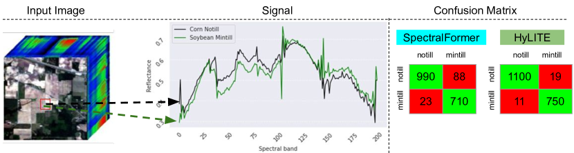
Figure 1: (Left) A image cube, with the spectral signals of two pixels from separate categories (‘notill’ and ‘mintill’) from the Indian Pines dataset (Graña et al., ). Observe how their spectral signature is highly similar. (Right) Confusion matrices of SpectralFormer (Hong et al., 2021) and HyLITE (Ours). SpectralFormer confuses these two classes, as it solely relies on the spectral signal. HyLITE disambiguates the classes by incorporating locality information.

The first deep HSI-based techniques adopted Convolutional Neural Networks (CNNs) to learn representations, either in a discriminative (Zhang et al., 2016; Li et al., 2017; Zhong et al., 2017; Nagasubramanian et al., 2019; Zhang et al., 2017; Paoletti et al., 2018; Zhao and Du, 2016) or generative manner (Wang et al., 2019; Ding et al., 2021). However, the performance of CNNs has been limited, due to the limited receptive field of CNNs (Dosovitskiy et al., 2020; Aleissaee et al., 2023), which cannot model long-range dependencies across spatial-spectral dimensions. To model long-range dependencies, self-attention is incorporated into CNNs (Mei et al., 2019; Sun et al., 2019; Zhu et al., 2020; Xie et al., 2021; Zheng et al., 2022), significantly increasing the receptive field of CNNs by enabling any pixel or spectrum to aggregate information from any other pixel or spectrum within the input cube. However, the receptive field of the backbone CNN representation is still too limited for HSI.

To overcome this limitation, most recent techniques rely solely on the Vision-Transformer (Dosovitskiy et al., 2020), which is a stack of multi-head self-attention modules. One notable example is SpectralFormer, which models the interactions across spectral bands to classify an input pixel (Hong et al., 2021). However, modeling spectral interactions alone can be insufficient for classification when pixels with different classes have very similar spectral signatures.

For instance, in Figure 1, we show the spectral signal of two pixels from the Indian Pines dataset (Graña et al., ), belonging to the ‘notill’ and ‘mintill’ classes, respectively. These pixels exhibit highly similar spectral signatures, which confuses the SpectralFormer (Hong et al., 2021). Fortunately, besides the spectral signal, images also provide the local information around a pixel, such as the representation of nearby pixels, which may help in disambiguating the target categories. Additionally, the global information within the signal, such as the set of potential categories present within the input image, could be useful. Hence, modeling the relationship between local and spectral information can help discriminate between the possible classes for a given pixel.

We propose a Hyperspectral Locality-aware Image TransformEr (HyLITE), which extends SpectralFormer in three major ways. Firstly, HyLITE models the relationships between local (spatial) and spectral representations, so that when spectral information is insufficient, local information can come into play. Secondly, we model the relationships between local and global representations with a novel regularization objective. Our regularization loss enforces local and distant pixels and spectra to aggregate information from each other, effectively improving representational capacity. Finally, we extensively evaluate our method on three standard HSI benchmarks and show that HyLITE establishes a new State-of-the-Art in HSI classification.

In summary, this paper makes three main contributions:

1. We propose Hyperspectral Locality-aware Image TransformEr (HyLITE), a novel architecture that can model the local-spectral relationships in data.

2. We equip HyLITE with a novel local-global regularization objective, to balance global and local spectral information.

3. We conduct experiments on three well-established benchmarks, and show that HyLITE significantly improves over the competitive SpectralFormer baseline, across all benchmarks and metrics. For example, we improve the overall accuracy by $10.83\%$ on Indian Pines (Graña et al., ), by $3.41\%$ on Houston2013 (hou, ), and by $6.64\%$ on Pavia (Graña et al., ).

2 Related Work

Vision Transformers. Vision-Transformers (ViTs) are a direct translation of language transformers in NLP (Manning and Schutze, 1999; Devlin et al., 2018) to computer vision (Dosovitskiy et al., 2020). The key building block of ViT is the self-attention layer (Vaswani et al., 2017), which consists of three subnetworks, namely Query, Key and Value networks. Query and Key networks compute the attention across the input signal, which is then used to modulate the input signal using the Value network. Since the release of ViT, many variants have been proposed (Touvron et al., 2021; Liu et al., 2021; Chen et al., 2020; Yuan et al., 2021; Bao et al., 2021; Wang et al., 2021). However, the majority of these are limited to processing RGB images. In this work, our model input consists of pre-processed image patches, which have a much lower spatial resolution (i.e., $7\times 7$ vs. $512\times 512$) and much higher spectral resolution (i.e., $200$ vs. $3$). These fundamental differences demand specialized architectures and loss functions. To that end, in this work, we develop new components combined with a novel loss function to learn the relationships between local and spectral information.

Image Transformers. ViTs have previously been used in state-of-the-art image classification architectures (Hong et al., 2021; Sun et al., 2022; Ibanez et al., 2022). Hong et al. (Hong et al., 2021) propose SpectralFormer, which treats each spectrum as a distinct token, and models spectrum-to-spectrum attention. However, HSI offers much more than spectrum-only information: it also contains spatial information, such as the local neighborhood of a pixel. To that end, Sun et al. (Sun et al., 2022) augment SpectralFormer with spatial attention. However, the mere combination of spectral and spatial attention is suboptimal. As we will demonstrate, regularizing local pixel representations with respect to global information matters greatly. Finally, Ibanez et al. (Ibanez et al., 2022) propose MAEST, which pre-trains a transformer backbone by predicting masked wavebands with Masked-AutoEncoders (He et al., 2022) prior to labeled fine-tuning. Such pre-training promotes locality and improves performance. However, self-supervised pre-training is computationally costly (Singh et al., 2023). Our HyLITE model combines spectral and spatial attention while also introducing local-global regularization, which achieves better performance without requiring pre-training.

3 Hyperspectral Locality-aware Image TransformEr

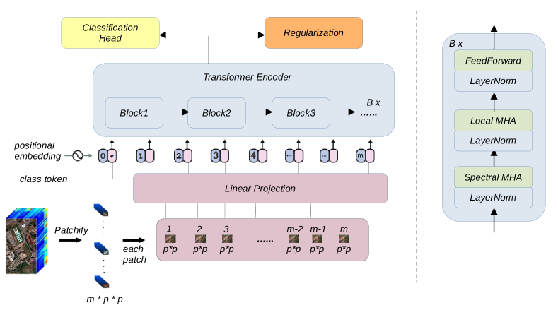
Figure 2: An overview of HyLITE. i). Preprocessing: The input image is patchified, linearly projected, and appended with a classifier token and a positional embedding. ii). Representation: The input is processed by identical spectral and local multi-head attention (MHA) blocks. iii). Classification: At the end, the representation of the classifier token is mapped to a distinct category, such as $\{grass,road\}$. iv). Regularization: To further promote locality, we apply our novel regularization on top of the learned token representations.

An overview of HyLITE is given in Figure 2. We strictly follow the protocol in (Hong et al., 2021), treating HSI as an image-level classification task. Given an image-label pair $({\bm{X}}\in\mathbb{R}^{p\times p\times m},{\bm{y}}\in\mathbb{R}^{c})$ where input ${\bm{X}}$ is a low-resolution square image with spatial resolution $p\times p$ (i.e., $7\times 7$) and spectral resolution $m$ (i.e., $200$), sampled from a high-resolution image by overlapping patchifying. Each patch is labeled by the category of its center pixel from $c$ potential classes, such as grass, road, etc. The goal is to train a vision transformer $f_{\theta}$ with parameters $\theta$ to predict the image label ${\bm{y}}^{\prime}=f_{\theta}({\bm{X}})$, where ${\bm{y}}^{\prime}\in\mathbb{R}^{c}$ denotes the predictions. We train our network in four main steps, which are detailed below.

1) Preprocessing. We first transform the input image by transposing and flattening it in the spatial dimension: ${\bm{X}}\in\mathbb{R}^{m\times p^{2}}$, thus yielding $m$ spectral tokens with dimensionality $p^{2}$: ${\bm{X}}=[{\bm{z}}^{1};{\bm{z}}^{2};...;{\bm{z}}^{m}]$ where ${\bm{z}}^{i}\in\mathbb{R}^{1\times p^{2}}$. We use ${\bm{X}}^{i}_{j}$ to denote the spectral token ${\bm{z}}^{i}$ at the $j$th transformer block. Next, we embed the tokens in $\mathbb{R}^{d}$ using a linear projection ${\bm{\mathsfit{W}}}\in\mathbb{R}^{p^{2}\times d}$, insert a learnable global classifier token ${\bm{z}}^{0}\in\mathbb{R}^{1\times d}$, and add a learnable position tensor ${\bm{\mathsfit{P}}}\in\mathbb{R}^{(m+1)\times d}$ to each token. As such, the first transformer block takes the form:

$${\bm{X}}_{0}=[{\bm{z}}^{0};{\bm{z}}^{1}{\bm{\mathsfit{W}}};...,{\bm{z}}^{m}{\bm{\mathsfit{W}}}]+{\bm{\mathsfit{P}}}$$ (1)

2) Representation. Each of the $B$ transformer blocks consists of three subsequent layers, namely Spectral-Attention $\text{S}(\cdot)$, Local-Attention $\text{L}(\cdot)$ and Feed-Forward $\text{F}(\cdot)$ layers, applied one after the other: ${\bm{X}}_{b}=\text{F}(\text{L}(\text{S}({\bm{X}}_{b-1})))\in\mathbb{R}^{(m+1)\times d}$ where $b=1\ldots B$. Before each layer, a LayerNorm (Ba et al., 2016) is applied, which we omit for clarity. Below, we detail each layer.

First, the spectral Multi-Head Attention (MHA) layer combines information from across the spectral dimension. It is implemented via self-attention. Formally:

$$\text{S}({\bm{X}})=\text{softmax}(\frac{({\bm{X}}{\bm{\mathsfit{W}}}_{q}^{s})({\bm{X}}{\bm{\mathsfit{W}}}_{k}^{s})^{T}}{\sqrt{d}})({\bm{X}}{\bm{\mathsfit{W}}}_{v}^{s})$$ (2)

where $\{{\bm{\mathsfit{W}}}_{q}^{s},{\bm{\mathsfit{W}}}_{k}^{s},{\bm{\mathsfit{W}}}_{v}^{s}\}$ are the linear query-key-value projections, respectively, all with tensor dimensionality $\mathbb{R}^{d\times d}$, where $\sqrt{d}$ is a scaling factor, and $\text{softmax}(\cdot)$ is the softmax operator.

Second, the local MHA layer combines information across the local (spatial) dimension. It is also implemented via self-attention. Formally:

$$\text{L}({\bm{X}})=\left(\text{softmax}(\frac{({\bm{X}}^{T}{\bm{\mathsfit{W}}}_{q}^{l})({\bm{X}}^{T}{\bm{\mathsfit{W}}}_{k}^{l})^{T}}{\sqrt{d}})({\bm{X}}^{T}{\bm{\mathsfit{W}}}_{v}^{l})\right)^{T}$$ (3)

where $\{{\bm{\mathsfit{W}}}_{q}^{l},{\bm{\mathsfit{W}}}_{k}^{l},{\bm{\mathsfit{W}}}_{v}^{l}\}$ are again linear query-key-value projections, with tensor dimensionality $\mathbb{R}^{(m+1)\times(m+1)}$.

Finally, the feed-forward layer consists of two linear layers and generates the output of each block with dimensionality $\mathbb{R}^{(m+1)\times d}$. After the last block, the token representations are passed to both a classification and regularization head.

3) Classification. We generate predictions by learning a linear mapping from the global token representation of the last layer to the classification labels: ${\bm{y}}^{\prime}={\bm{X}}^{0}_{B}C$, where $C\in\mathbb{R}^{d\times c}$ is the classifier head. Using the predictions and the final representations, the model is trained by minimizing the following objective:

$$\mathcal{O}=\text{CE}({\bm{y}},{\bm{y}}{\prime})+\lambda\cdot\text{Reg}({\bm{X}}_{B})$$ (4)

where $\text{CE}(\cdot)$ is the standard cross-entropy loss, $\text{Reg}(\cdot)$ is our novel local-global regularization objective, and $\lambda$ attenuates the regularization strength. In the remainder of this paper, we set $\lambda=1$. The effects of different $\lambda$ values are reported in the supplemental materials.

4) Regularization. During the training of HyLITE, we observed that the spectral tokens mostly attend to their self-representation, hence focusing on the local context and ignoring the global context. Moreover, the global token mostly attends to a few specific tokens, ignoring the rest of the local context. This indicates that the spectral and global token representations diverge throughout the blocks, and hence we name this phenomenon "attentional divergence". To prevent such divergence and improve performance, we propose the following regularization objective:

$$\text{Reg}({\bm{X}}_{B})=\left\|{\bm{X}}_{B}^{0}-\frac{1}{m}\sum_{i=1}^{m}{\bm{X}}_{B}^{i}\right\|_{2}^{2}$$ (5)

To minimize this loss function, the global output token ${\bm{X}}_{B}^{0}$ should be close to the center of the spectral tokens. Hence, the gradients will nudge the representations of the global and spectral tokens closer together, causing them to converge rather than diverge, and aggregating information from each other, thus incorporating globality in the learning process. Notably, the use of a learned global token works differently (and performs much better) than simply applying average pooling over all spectral tokens. It better balances acquired global and local knowledge, while average pooling might cause information loss. As we will demonstrate, this approach has a significant positive effect on classification performance.

4 Experimental Setup

We evaluate our method on multiple datasets, with multiple metrics, and against multiple strong baselines. The supplementary provides further details on implementation and setup.

$\triangleright$Datasets: We evaluate our model on three well-established HSI datasets. i). Indian Pines (Graña et al., ): consists of $224$ spectral bands with $145\times 145$ spatial resolution. It includes $16$ classes, $695$ training, and $9k$ testing samples. ii). Houston2013 (hou, ): consists of $144$ spectral bands with $349\times 1905$ spatial resolution. It includes $15$ classes, $2k$ training, and $12k$ testing samples. iii). Pavia University (Graña et al., ): consists of $103$ spectral bands with $610\times 340$ spatial resolution. It includes $15$ classes, $3k$ training, and $40k$ testing samples.

$\triangleright$Metrics: We rely on the standard metrics, namely Overall Accuracy (OA), Average Accuracy (AA) and Kappa Coefficient ($k$). OA denotes the total number of correctly predicted samples over all samples, while AA denotes the average accuracy of each class.

$\triangleright$Baselines: We mainly compare HyLITE against the state-of-the-art methods SpectralFormer (Hong et al., 2021) and $MAEST^{*}$ (Ibanez et al., 2022). We also compare against conventional methods (i.e., kNN, RF), and CNN-based techniques (N-D CNNs) for the sake of completeness.

5 Image Classification

5.1 Comparison to the State-of-the-Art

Firstly, we compare our method against several baselines from the HSI literature in Table 5.1. We use the exact same evaluation procedure as used in (Hong et al., 2021) to get a fair comparison. We can make four observations based on these results: i). HyLITE achieves State-of-the-Art performance by a significant margin across all three datasets and all three metrics. ii). Our performance surpasses that of the most competitive baseline, SpectralFormer, by $3-10\%$ in overall accuracy in the respective benchmarks, confirming our hypothesis that SpectralFormer lacks crucial locality information. iii). Third, the improvement of HyLITE is particularly noteworthy on the Indian Pines dataset, with Overall Accuracy and Average Accuracy improving by $10.83\%$ and $9.30\%$, respectively. This suggests that adding locality information helps to learn more effectively from small amounts of training data, since Indian Pines has the smallest amount of training data among the three benchmarks, with only $695$ instances. We will further explore this in the next section. iv). HyLITE even outperforms $MAEST$ (Ibanez et al., 2022), which performs computationally expensive self-supervised pre-training prior to fine-tuning. This indicates that once discriminative inductive biases are present within the model, self-supervised pre-training is no longer needed.

We conclude that incorporating locality is highly valuable for image classification, as evidenced by the significant improvement over competitive baselines across all benchmarks.

	Indian Pines			Houston2013			Pavia University
	OA	AA	Kappa	OA	AA	Kappa	OA	AA	Kappa
kNN	59.17	63.90	0.54	77.30	78.28	0.75	70.53	79.68	0.62
RF	69.80	76.78	0.65	77.48	80.35	0.75	69.67	80.18	0.62
SVM	72.36	83.16	0.68	76.91	78.99	0.79	70.82	84.44	0.64
1-10 1-D CNN	70.43	79.60	0.66	80.04	82.74	0.78	75.50	86.26	0.69
2-D CNN	75.89	86.64	0.72	83.72	84.35	0.82	86.05	88.99	0.81
RNN	70.66	76.37	0.66	82.23	85.04	0.81	77.13	84.29	0.71
miniGCN	75.11	78.03	0.71	81.71	83.09	0.80	79.79	85.07	0.73
1-10 ViT	71.86	78.97	0.68	80.41	82.50	0.78	76.99	80.22	0.70
SpectralFormer	78.97	85.39	0.76	85.08	86.39	0.83	84.64	86.75	0.79
HyLITE (Ours)	$89.80$	$94.69$	$0.88$	$88.49$	$89.74$	$0.87$	$91.28$	$92.25$	$0.88$
$\Delta$	$10.83$	$9.30$	$0.12$	$3.41$	$3.35$	$0.03$	$6.64$	$5.50$	$0.08$
1-10 $MAEST$	82.12	87.63	0.79	83.61	84.89	0.82	87.20	89.91	0.83

Table 1: Comparison against the State-of-the-Art. We provide the results from all baselines, as well as the performance gap ($\Delta$) with SpectralFormer. Our model consistently outperforms all techniques by a wide margin across all datasets and evaluation metrics. Notably, our model most significantly outperforms SpectralFormer when the training set is small (e.g., only $695$ training instances in Indian Pines). Surprisingly, our model even outperforms the computationally much more expensive self-supervised pre-training approach of $MAEST$. These findings support our hypothesis that spatial locality plays a crucial role in image classification.

5.2 Evaluation of Sample Efficiency

In the previous section, we focused on learning on all available data. However, in imaging, sample efficiency matters greatly, as data collection and annotation are costly. To that end, we compare the performance of HyLITE with SpectralFormer on Indian Pines, by varying the size of the training set within $\{10\%,20\%,...,100\%\}$. We repeat the experiment $4$ times with different random training samples, and present the mean and standard deviation in Figure 3.

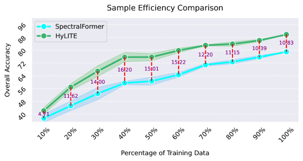
Figure 3: Comparing the sample efficiency of HyLITE and SpectralFormer (Hong et al., 2021) on Indian Pines (Graña et al., ). HyLITE outperforms across all subsets, confirming the efficacy of locality for learning from limited examples.

From this, we can make two observations: i). The performance of both models degrades drastically as the size of the training set shrinks (i.e., $10\%$). This is expected, as Vision-Transformers require a sufficient number of exemplars to generalize. ii). HyLITE is always superior to SpectralFormer across all subsets. This indicates that incorporating locality is useful in improving the sample efficiency of image classifiers.

Hence, we conclude that incorporating locality not only improves accuracy, but also improved sample efficiency of imaging, which is promising for low-shot learning applications.

5.3 Ablation Analysis

We ablate the position and the components of HyLITE in Table 5.3.

	Indian Pines			Houston2013			Pavia University
	OA	AA	Kappa	OA	AA	Kappa	OA	AA	Kappa
Positional Embedding
1-10 No Embedding	79.63	85.35	0.77	84.09	85.96	0.83	84.69	87.18	0.79
Fixed Embedding	85.30	88.56	0.83	83.46	85.26	0.82	87.36	85.64	0.83
Learned Embedding	89.80	94.69	0.88	88.49	89.74	0.88	91.28	92.25	0.88
Components
1-10 local-att(✗) & local-reg(✗)	78.97	85.39	0.76	85.08	86.39	0.83	84.64	86.75	0.79
local-att(✓) & local-reg(✗)	85.37	90.09	0.83	87.69	89.18	0.87	87.78	91.06	0.84
local-att(✗) & local-reg(✓)	83.00	89.40	0.81	87.13	88.33	0.86	87.76	91.72	0.84
local-att(✓) & local-reg(✓)	89.80	94.69	0.88	88.49	89.74	0.88	91.28	92.25	0.88

Table 2: Ablation Study. Learning the positional embedding, as well as combining our local attention (local-att) with local-global regularization (local-reg) matters.

Positional Embedding. Here, we try to understand the contribution of positional information in HyLITE. First, removing positional information leads to a drastic performance drop, as expected. This indicates HyLITE greatly utilizes location information. Secondly, learning positional information yields much better performance than fixing positional information. This indicates HyLITE learns to adjust the relative contribution of each token within the input.

Components. We ablate the local attention (local-att) and regularization (local-reg) components to understand their relative contribution. Firstly, including either local attention or local-global regularization helps greatly. However, incorporating both leads to a significant gain, indicating that regularizing the local-attention representation matters in image classification.

We conclude that HyLITE is able to incorporate positional information efficiently, and regularizing the local-attentional representation is critical for classification accuracy.

5.4 Category-level Analysis

Here, we provide a category-level comparison with SpectralFormer on Indian Pines. Results are presented in Figure 4. The comparison results on Houston2013 and Pavia University datasets are presented in Section 3 of the supplementary material.

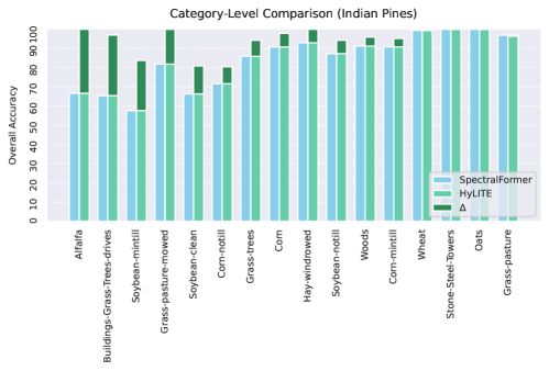
Figure 4: Category-level comparison to the SpectralFormer on Indian Pines. The contribution of HyLITE is generic, with fine-grained categories of ‘Alfalfa’, ‘Buildings-Grass-Trees-drives’, and ‘Soybean-mintill’ receiving the highest benefits.

As can be seen, the contribution of HyLITE is generic, as it improves over all (non-saturated) categories. The improvement is more pronounced for easily misclassified classes by SpectralFormer, such as ‘Alfalfa’, ‘Buildings-Grass-Trees-drives’, and ‘Soybean-mintill’. This indicates that local, fine-grained details matter to distinguish such categories.

5.5 Architectural Analysis

In this section, we provide further analysis to justify architectural choices in this paper (see Section 3). The results are presented in Table 5.5.

	Indian Pines			Houston2013			Pavia University
	OA	AA	Kappa	OA	AA	Kappa	OA	AA	Kappa
Order of Attention
1-10 Local-to-Spectral	87.44	92.25	0.86	87.14	88.18	0.86	85.60	91.29	0.81
Spectral-to-Local	89.80	94.69	0.88	88.49	89.74	0.87	91.28	92.25	0.88
Global Token
1-10 Local-token	83.54	92.61	0.81	85.85	87.26	0.85	91.05	92.16	0.88
Spectral-token	89.80	94.69	0.88	88.49	89.74	0.87	91.28	92.25	0.88
Fusion
1-10 Class-level	81.05	89.86	0.79	86.05	87.83	0.85	87.41	88.20	0.83
Feature-level	89.80	94.69	0.88	88.49	89.74	0.87	91.28	92.25	0.88

Table 3: Architectural Analysis. It is important to incorporate spectral attention prior to local, using a global spectral token as opposed to local, and combining representations at the feature-level rather than class-level.

Order of Attention. Firstly, we observe that the order of attentional blocks matters. Including spectral information prior to spatial information leads to better performance. This is expected, since in imaging, most of the information is present within the spectrum, and the input image may exhibit low spatial resolution.

Global Token. Originally, the additional global classifier token for HyLITE is spectral. Here, we test the performance with local tokens by transposing the dimensions and adding a global classifier token to the local dimension. We observe that pooling the representation from the spectral token matters, as opposed to local. This indicates that even though locality matters, spectral information carries more discriminative information for classification.

Fusion. In HyLITE, we combine spectral and local information directly within the block (i.e., feature-level). We also experiment with late-fusion, where one model only includes spectral attention and the other only local attention, whose output is combined at the class-level. As is evident from Table 5.5, feature-level fusion outperforms the class-level counterpart by a large-margin, indicating the importance of spectral-to-local interactions for HSI.

6 Conclusion

In this paper, we tackled image classification. Motivated by the limited local information in state-of-the-art image transformers, we incorporated the locality by attending to the local pixels as well as regularizing the local-to-global representations with our novel loss function. Evaluated on three well-established benchmarks, we observe that HyLITE is highly accurate, as it improves state-of-the-art across all datasets and all metrics. Secondly, we observe that HyLITE is highly efficient, as it learns much better from less number of examples. Finally, we highlight the importance of our architectural choices, for a principled inclusion of locality into transformers. We conclude that locality is crucial for image classification.

Acknowledgements. This work was supported by the Dutch Science Foundation (NWO) under grant 700. Furthermore, we are grateful for the valuable and constructive feedback provided by our anonymous reviewers and the meta reviewer. Their input significantly contributed to the enhancement of our manuscript.

References

- (1) 2013 IEEE GRSS Data Fusion Contest – Fusion of Hyperspectral and LiDAR Data. URL https://hyperspectral.ee.uh.edu/?page_id=459.
- Aleissaee et al. (2023) Abdulaziz Amer Aleissaee, Amandeep Kumar, Rao Muhammad Anwer, Salman Khan, Hisham Cholakkal, Gui-Song Xia, and Fahad Shahbaz Khan. Transformers in remote sensing: A survey. Remote Sensing, 15(7):1860, 2023.
- Ba et al. (2016) Jimmy Lei Ba, Jamie Ryan Kiros, and Geoffrey E Hinton. Layer normalization. arXiv preprint arXiv:1607.06450, 2016.
- Bao et al. (2021) Hangbo Bao, Li Dong, Songhao Piao, and Furu Wei. Beit: Bert pre-training of image transformers. arXiv preprint arXiv:2106.08254, 2021.
- Chen et al. (2020) Mark Chen, Alec Radford, Rewon Child, Jeffrey Wu, Heewoo Jun, David Luan, and Ilya Sutskever. Generative pretraining from pixels. In International conference on machine learning, pages 1691–1703. PMLR, 2020.
- Dale et al. (2013) Laura M Dale, André Thewis, Christelle Boudry, Ioan Rotar, Pierre Dardenne, Vincent Baeten, and Juan A Fernández Pierna. Hyperspectral imaging applications in agriculture and agro-food product quality and safety control: A review. Applied Spectroscopy Reviews, 48(2):142–159, 2013.
- Devlin et al. (2018) Jacob Devlin, Ming-Wei Chang, Kenton Lee, and Kristina Toutanova. Bert: Pre-training of deep bidirectional transformers for language understanding. arXiv preprint arXiv:1810.04805, 2018.
- Ding et al. (2021) Fanchang Ding, Baofeng Guo, Xiangxiang Jia, Haoyu Chi, and Wenjie Xu. Improving gan-based feature extraction for hyperspectral images classification. Journal of Electronic Imaging, 30(6):063011–063011, 2021.
- Dosovitskiy et al. (2020) Alexey Dosovitskiy, Lucas Beyer, Alexander Kolesnikov, Dirk Weissenborn, Xiaohua Zhai, Thomas Unterthiner, Mostafa Dehghani, Matthias Minderer, Georg Heigold, Sylvain Gelly, et al. An image is worth 16x16 words: Transformers for image recognition at scale. arXiv preprint arXiv:2010.11929, 2020.
- Furbank et al. (2021) Robert T Furbank, Viridiana Silva-Perez, John R Evans, Anthony G Condon, Gonzalo M Estavillo, Wennan He, Saul Newman, Richard Poiré, Ashley Hall, and Zhen He. Wheat physiology predictor: predicting physiological traits in wheat from hyperspectral reflectance measurements using deep learning. Plant Methods, 17:1–15, 2021.
- Goetz (2009) Alexander FH Goetz. Three decades of hyperspectral remote sensing of the earth: A personal view. Remote sensing of environment, 113:S5–S16, 2009.
- (12) M Graña, MA Veganzons, and B Ayerdi. Hyperspectral remote sensing scenes. Hyperspectral Remote Sensing Scenes - Grupo de Inteligencia Computacional (GIC). URL https://www.ehu.eus/ccwintco/index.php/Hyperspectral_Remote_Sensing_Scenes.
- He et al. (2022) Kaiming He, Xinlei Chen, Saining Xie, Yanghao Li, Piotr Dollár, and Ross Girshick. Masked autoencoders are scalable vision learners. In Proceedings of the IEEE/CVF Conference on Computer Vision and Pattern Recognition, pages 16000–16009, 2022.
- Hong et al. (2021) Danfeng Hong, Zhu Han, Jing Yao, Lianru Gao, Bing Zhang, Antonio Plaza, and Jocelyn Chanussot. Spectralformer: Rethinking hyperspectral image classification with transformers. IEEE Transactions on Geoscience and Remote Sensing, 60:1–15, 2021.
- Ibanez et al. (2022) Damian Ibanez, Ruben Fernandez-Beltran, Filiberto Pla, and Naoto Yokoya. Masked auto-encoding spectral–spatial transformer for hyperspectral image classification. IEEE Transactions on Geoscience and Remote Sensing, 60:1–14, 2022.
- Jakubczyk et al. (2022) Kacper Jakubczyk, Barbara Siemiątkowska, Rafał Więckowski, and Jerzy Rapcewicz. Hyperspectral imaging for mobile robot navigation. Sensors, 23(1):383, 2022.
- Li et al. (2017) Ying Li, Haokui Zhang, and Qiang Shen. Spectral–spatial classification of hyperspectral imagery with 3d convolutional neural network. Remote Sensing, 9(1):67, 2017.
- Liu et al. (2021) Ze Liu, Yutong Lin, Yue Cao, Han Hu, Yixuan Wei, Zheng Zhang, Stephen Lin, and Baining Guo. Swin transformer: Hierarchical vision transformer using shifted windows. In Proceedings of the IEEE/CVF international conference on computer vision, pages 10012–10022, 2021.
- Manning and Schutze (1999) Christopher Manning and Hinrich Schutze. Foundations of statistical natural language processing. MIT press, 1999.
- Mei et al. (2019) Xiaoguang Mei, Erting Pan, Yong Ma, Xiaobing Dai, Jun Huang, Fan Fan, Qinglei Du, Hong Zheng, and Jiayi Ma. Spectral-spatial attention networks for hyperspectral image classification. Remote Sensing, 11(8):963, 2019.
- Nagasubramanian et al. (2019) Koushik Nagasubramanian, Sarah Jones, Asheesh K Singh, Soumik Sarkar, Arti Singh, and Baskar Ganapathysubramanian. Plant disease identification using explainable 3d deep learning on hyperspectral images. Plant methods, 15:1–10, 2019.
- Paoletti et al. (2018) Mercedes E Paoletti, Juan Mario Haut, Ruben Fernandez-Beltran, Javier Plaza, Antonio J Plaza, and Filiberto Pla. Deep pyramidal residual networks for spectral–spatial hyperspectral image classification. IEEE Transactions on Geoscience and Remote Sensing, 57(2):740–754, 2018.
- Singh et al. (2023) Mannat Singh, Quentin Duval, Kalyan Vasudev Alwala, Haoqi Fan, Vaibhav Aggarwal, Aaron Adcock, Armand Joulin, Piotr Dollár, Christoph Feichtenhofer, Ross Girshick, et al. The effectiveness of mae pre-pretraining for billion-scale pretraining. arXiv preprint, 2023.
- Sun et al. (2019) Hao Sun, Xiangtao Zheng, Xiaoqiang Lu, and Siyuan Wu. Spectral–spatial attention network for hyperspectral image classification. IEEE Transactions on Geoscience and Remote Sensing, 58(5):3232–3245, 2019.
- Sun et al. (2022) Le Sun, Guangrui Zhao, Yuhui Zheng, and Zebin Wu. Spectral–spatial feature tokenization transformer for hyperspectral image classification. IEEE Transactions on Geoscience and Remote Sensing, 60:1–14, 2022.
- Touvron et al. (2021) Hugo Touvron, Matthieu Cord, Matthijs Douze, Francisco Massa, Alexandre Sablayrolles, and Hervé Jégou. Training data-efficient image transformers & distillation through attention. In International conference on machine learning, pages 10347–10357. PMLR, 2021.
- Transon et al. (2018) Julie Transon, Raphaël d’Andrimont, Alexandre Maugnard, and Pierre Defourny. Survey of hyperspectral earth observation applications from space in the sentinel-2 context. Remote Sensing, 10(2):157, 2018.
- Trierscheid et al. (2008) Marina Trierscheid, Johannes Pellenz, Dietrich Paulus, and Dirk Balthasar. Hyperspectral imaging or victim detection with rescue robots. In 2008 IEEE International Workshop on Safety, Security and Rescue Robotics, pages 7–12. IEEE, 2008.
- Vaswani et al. (2017) Ashish Vaswani, Noam Shazeer, Niki Parmar, Jakob Uszkoreit, Llion Jones, Aidan N Gomez, Łukasz Kaiser, and Illia Polosukhin. Attention is all you need. Advances in neural information processing systems, 30, 2017.
- Wang et al. (2019) Dongyi Wang, Robert Vinson, Maxwell Holmes, Gary Seibel, Avital Bechar, Shimon Nof, and Yang Tao. Early detection of tomato spotted wilt virus by hyperspectral imaging and outlier removal auxiliary classifier generative adversarial nets (or-ac-gan). Scientific reports, 9(1):1–14, 2019.
- Wang et al. (2021) Wenhai Wang, Enze Xie, Xiang Li, Deng-Ping Fan, Kaitao Song, Ding Liang, Tong Lu, Ping Luo, and Ling Shao. Pyramid vision transformer: A versatile backbone for dense prediction without convolutions. In Proceedings of the IEEE/CVF international conference on computer vision, pages 568–578, 2021.
- Xie et al. (2015) Chuanqi Xie, Yongni Shao, Xiaoli Li, and Yong He. Detection of early blight and late blight diseases on tomato leaves using hyperspectral imaging. Scientific reports, 5(1):1–11, 2015.
- Xie et al. (2021) Zhuojun Xie, Jianwen Hu, Xudong Kang, Puhong Duan, and Shutao Li. Multilayer global spectral–spatial attention network for wetland hyperspectral image classification. IEEE Transactions on Geoscience and Remote Sensing, 60:1–13, 2021.
- Yuan et al. (2021) Li Yuan, Yunpeng Chen, Tao Wang, Weihao Yu, Yujun Shi, Zi-Hang Jiang, Francis EH Tay, Jiashi Feng, and Shuicheng Yan. Tokens-to-token vit: Training vision transformers from scratch on imagenet. In Proceedings of the IEEE/CVF international conference on computer vision, pages 558–567, 2021.
- Zhang et al. (2017) Haokui Zhang, Ying Li, Yuzhu Zhang, and Qiang Shen. Spectral-spatial classification of hyperspectral imagery using a dual-channel convolutional neural network. Remote sensing letters, 8(5):438–447, 2017.
- Zhang et al. (2016) Liangpei Zhang, Lefei Zhang, and Bo Du. Deep learning for remote sensing data: A technical tutorial on the state of the art. IEEE Geoscience and remote sensing magazine, 4(2):22–40, 2016.
- Zhao and Du (2016) Wenzhi Zhao and Shihong Du. Spectral–spatial feature extraction for hyperspectral image classification: A dimension reduction and deep learning approach. IEEE Transactions on Geoscience and Remote Sensing, 54(8):4544–4554, 2016.
- Zheng et al. (2022) Xiangtao Zheng, Hao Sun, Xiaoqiang Lu, and Wei Xie. Rotation-invariant attention network for hyperspectral image classification. IEEE Transactions on Image Processing, 31:4251–4265, 2022.
- Zhong et al. (2017) Zilong Zhong, Jonathan Li, Zhiming Luo, and Michael Chapman. Spectral–spatial residual network for hyperspectral image classification: A 3-d deep learning framework. IEEE Transactions on Geoscience and Remote Sensing, 56(2):847–858, 2017.
- Zhu et al. (2020) Minghao Zhu, Licheng Jiao, Fang Liu, Shuyuan Yang, and Jianing Wang. Residual spectral–spatial attention network for hyperspectral image classification. IEEE Transactions on Geoscience and Remote Sensing, 59(1):449–462, 2020.