Shear viscosity of rotating, hot, and dense spin-half fermionic systems from quantum field theory

Abstract

In this study, we calculate the shear viscosity for rotating fermions with spin-half under conditions of high temperature and density. We employ the Kubo formalism, rooted in finite-temperature quantum field theory, to compute the field correlation functions essential for this evaluation. The one-loop diagram pertinent to shear viscosity is analyzed within the context of curved space, utilizing tetrad formalism as an effective approach in cylindrical coordinates. Our findings focus on extremely high angular velocities, ranging from 0.1 to 1 GeV, which align with experimental expectations. Furthermore, we explore the inter-relationship between the chemical potential and angular velocity within the scope of this study.

I Introduction

The study of Quark Gluon Plasma (QGP), formed during heavy-ion collisions and particularly in high electromagnetic fields or significant angular velocities, is a critical area of research [1, 2, 3, 4, 5, 6, 7, 8, 9, 10]. High angular velocities in off-center collisions, leading to angular momentum of $10^{3\sim 5}\hbar$, have been observed by the STAR collaboration, adding complexity to the study of these extreme matter states [11]. Advances from RHIC and LHC experiments show that QGP rapidly evolves from a glasma state to equilibrium, and then into hadrons [2, 3, 5, 4]. Theoretically, relativistic hydrodynamics supports the view of QGP as the smallest fluid droplets with almost perfect fluidity, leading to new explorations in off-equilibrium hydrodynamics [12, 13, 14, 15, 16, 17].

Furthermore, measurements by the STAR collaboration indicate that emitted particles, such as $\Lambda$ hyperons, show spin polarization, highlighting QGP as the most vortical system observed in heavy-ion collisions to date [18, 19, 20, 21, 22, 23]. This spin alignment, corresponding with their angular momentum, has intensified interest in the underlying dynamics. Extensive research using various methodologies has been conducted to explore these dynamics [24, 25, 26, 27, 28, 29, 30, 31, 32, 33, 34, 35, 36, 37, 38, 39, 40, 41, 42, 43, 44, 45, 46, 47, 48, 49, 50, 51, 38, 41, 52, 53, 35, 36, 37, 54, 55, 56, 57, 58, 59, 39, 60, 42, 61, 62, 63, 64, 65, 66, 57, 67, 68, 69, 40, 41, 70, 71, 72, 73, 74]. Recent reviews have provided insights into both local and global spin polarization, and developments in spin hydrodynamics, from holographic and quantum field theoretical perspectives, have further enriched this field of study. Recent trends in the field have expanded to include the exploration of spin polarization within nuclear matter and its interaction with electromagnetic fields. These new measurements have significantly enhanced our comprehension of the Quark Gluon Plasma (QGP), concurrently driving numerous theoretical developments. Consequently, the study of QGP, particularly in extreme conditions, continues to be a dynamic and intriguing area of scientific research.

Theoretical research predicts numerous intriguing phenomena in extreme conditions, like the chiral vortical effect [25, 75, 76, 77], chiral vortical wave [78], mass splitting under rotation [79], magnetic chiral density wave [80], and vortical effects in AdS space [81]. These anomalous processes, reliant on experimental signatures, are observable in heavy-ion collision experiments. High angular velocities in the QCD medium provide an opportunity to explore these properties in detail, facilitating the extraction of experimental signatures. Another intriguing research area is the QCD phase diagram under rotation [11, 82, 83]. Studies have shown that rotation affects the confining and deconfining phases of QGP. For instance, the deconfining transition occurs at a specific distance from the rotation axis [82]. There is evidence of a mixed inhomogeneous phase with spatially separated confinement and deconfinement regions, leading to the prediction of two deconfining temperatures. In the context of lattice SU(3) gauge theory, the isothermal moment of inertia for a rigidly rotating QGP has been computed, revealing negative values below the supervortical temperature, which is 1.5 times the critical temperature [84]. This suggests that a rigidly rotating system becomes thermodynamically unstable beyond a certain temperature.

In the study of rotating QCD matter, transport coefficients are vital for hydrodynamic simulations [56]. These coefficients can be calculated using approaches like kinetic theory, based on the relativistic Boltzmann equation [34, 33], and field theoretic formulations, which focus on correlation function calculations [70, 85, 86, 87, 88]. Recent studies using Zubarev’s non-equilibrium statistical operator formalism have reported Kubo formulas for various transport coefficients in first-order spin hydrodynamics, introducing new coefficients such as rotational viscosity and boost heat conductivity in addition to traditional coefficients like shear viscosity, bulk viscosity, and thermal conductivity [56]. These formulations are essential for understanding the impact of rotational effects, which induce background torsion, interacting with fermionic fields. However, gauge fields do not couple with torsion due to the SU(3)${}_{\text{c}}$ gauge invariance [89, 70]. The influence of rotation in field theory is akin to the effects of a background magnetic field, altering the propagator’s translational symmetry between two spacetime points [90, 91, 92, 93]. For magnetic fields, this alteration manifests as the Schwinger phase factor, an exponential function indicating a phase shift. In a rotating environment, a similar factor appears in the fermion propagator. Interestingly, translational symmetry is restored at high angular velocities, simplifying the computation of field correlation functions [94].

In our study, we investigate how finite rotation impacts transport coefficients, particularly focusing on shear viscosity in a fermion-dominated medium subject to high angular velocity. Employing the Kubo formalism, we incorporate the influence of rotation in our calculations by using the momentum space propagator for fermions, derived via the Fock-Schwinger method. The role of angular velocity is notably apparent in two areas: it modifies the distribution function through the summation of Matsubara frequencies, and it is also present in the numerator of the shear viscosity expression via trace evaluations. Our initial findings suggest that both temperature and angular velocity lead to an increase in shear viscosity, while an increase in chemical potential results in its reduction. Interestingly, the study uncovers that chemical potential and angular velocity, though functionally similar, exert opposite effects on shear dissipation within fermionic systems.

This paper is structured as follows: Section II explores the dynamics of fermions in a rotating environment. Next, in Section III, we delve into the calculations of the spectral function and the shear viscosity of fermions. Section IV is devoted to discussing the results of our study. Finally, we provide a summary in Section V.

II Fermions in a rotating medium

In this section, we provide a concise introduction to the behavior of fermions in a rotating setting. To investigate this complex system, our approach will be based in curved spacetime. The metric tensor, akin to that of a curved spacetime, serves as a useful tool for characterizing the geometric properties of the region generated following non-central collisions, which rotates at an angular velocity $\Omega$ about the $z$-axis. For this specific system, the metric tensor $g^{\mu\nu}$ is represented by

$$g_{\mu\nu}=\begin{pmatrix}1-\left(x^{2}+y^{2}\right)\Omega^{2}&y\Omega&-x\Omega&0\\ y\Omega&-1&0&0\\ -x\Omega&0&-1&0\\ 0&0&0&-1\end{pmatrix},$$ (1)

and the Dirac equation describing a massive fermion with mass $m$ and spin-$\frac{1}{2}$ in cylindrical coordinates [94, 95] is

$$\left(i\widetilde{\gamma}^{\mu}\widetilde{D}_{\mu}-m\right)\psi=0\,,$$ (2)

where $\widetilde{\gamma}^{\mu}$ are the gamma matrices and $\widetilde{D}_{\mu}$ is the covariant derivative

$$\widetilde{D}_{\mu}=\partial_{\mu}+\Gamma_{\mu}\,.$$ (3)

Here, $\Gamma_{\mu}=(1/8)\,\omega_{\mu ab}\big{[}\gamma^{a},\gamma^{b}\big{]}$ is the affine connection with $\omega_{\mu ab}$ being the spin connection. To compute $\omega_{\mu ab}$ one has to use the definition of vierbein (also known as tetrad) and metric tensor $g_{\mu\nu}$ which are given as

$$e_{a}^{~{}\mu} = \delta_{a}^{~{}\mu}-\delta_{a}^{~{}0}\delta_{i}^{~{}\mu}v_{i}\,,\quad\text{with}\quad(i=1,2,3)$$

$$e^{a}_{~{}\mu} = \delta^{a}_{~{}\mu}+\delta^{a}_{~{}i}\delta^{0}_{~{}\mu}v_{i}\,,$$

$$g_{\mu\nu} = \eta_{ab}e^{a}_{~{}\mu}e^{b}_{~{}\nu}\,,$$ (4)

where $\eta_{ab}=\text{diag}(1,-1,-1,-1)$ is the Minkowski spacetime metric tensor. Thus, one obtains

$$\omega_{\mu ab}=g_{\alpha\beta}e_{a}^{~{}\alpha}\left[\partial_{\mu}e_{b}^{~{}\beta}+\Gamma^{\beta}_{~{}\mu\nu}e_{b}^{~{}\nu}\right],$$ (5)

where $\Gamma^{\beta}_{~{}\mu\nu}$ is the Christoffel symbol defined as [96]

$$\Gamma^{\beta}_{~{}\mu\nu}=\frac{g^{\beta\alpha}}{2}\left[\partial_{\nu}g_{\alpha\mu}+\partial_{\mu}g_{\alpha\nu}-\partial_{\alpha}g_{\mu\nu}\right].$$ (6)

In curved spacetime the energy-momentum tensor is given as [95]

$$T^{\mu\nu}=\frac{i}{4}\left(\overline{\psi}\widetilde{\gamma}^{\mu}\widetilde{D}^{\nu}\psi+\overline{\psi}\widetilde{\gamma}^{\nu}\widetilde{D}^{\mu}\psi\right)+\rm{h.c},$$ (7)

where $\psi$ and $\overline{\psi}$ are the Dirac field operator and its conjugate, respectively, and h.c denotes the Hermitian conjugate. In a uniformly rotating frame, $\widetilde{D}^{\mu}$ is

$$\widetilde{D}_{\mu}=\left(\partial_{t}-i\frac{\Omega\Sigma_{3}}{2},-\partial_{x},-\partial_{y},-\partial_{z}\right),$$ (8)

where $\Sigma_{3}=(i/2)\left[\gamma^{1},\gamma^{2}\right]$. The spacetime dependent gamma matrices $\widetilde{\gamma}^{\mu}$ [95, 94] in tetrad system present in Eq. (7) are defined as

$$\widetilde{\gamma}^{0}=\gamma^{0}\,,\quad\quad\quad~{}\quad\widetilde{\gamma}_{0}=\gamma^{0}-x\Omega\gamma^{2}+y\Omega\gamma^{1}\,,$$

$$\widetilde{\gamma}^{1}=\gamma^{1}+y\Omega\gamma^{0}\,,\quad\widetilde{\gamma}_{1}=-\gamma^{1}\,,$$

$$\widetilde{\gamma}^{2}=\gamma^{2}-x\Omega\gamma^{0}\,,\quad\widetilde{\gamma}_{2}=-\gamma^{2}\,,$$

$$\widetilde{\gamma}^{3}=\gamma^{3}\,,\quad\quad\quad~{}~{}\quad\widetilde{\gamma}_{3}=-\gamma^{3}\,,$$ (9)

where $\gamma^{\mu}$ are the gamma matrices in Minkowski space. In off-central heavy-ion collisions the direction of rotation is perpendicular to the reaction $(x-y)$ plane. Following the above mentioned details, the Lagrangian with finite chemical potential $\mu$ for a medium rotating with constant angular velocity $\Omega$ is expressed as [97]

$$\mathcal{L}=\overline{\psi}\left[i\gamma^{\mu}\partial_{\mu}+\gamma^{0}\left(\Omega J_{z}+\mu\right)-m\right]\psi\,,$$ (10)

with $J_{z}$ being the third component of the total angular momentum given by $\vec{J}=\vec{x}\times\vec{p}+\vec{S}$ where $\vec{S}=(1/2)\begin{pmatrix}\vec{\sigma}&0\\ 0&\vec{\sigma}\end{pmatrix}$. The fermion propagator in the momentum space derived from the above Lagrangian using Fock-Schwinger method is given by [93, 94]

$$S(p) = \frac{\big{(}p_{0}+\frac{\Omega}{2}-p_{z}+ip_{\perp}\big{)}\big{(}\gamma_{0}+\gamma_{3}\big{)}+m\big{(}1+\gamma_{5}\big{)}}{\big{(}p_{0}+\frac{\Omega}{2}\big{)}^{2}-\vec{p}^{2}-m^{2}+i\epsilon}\mathcal{O}^{+}+\frac{\big{(}p_{0}-\frac{\Omega}{2}+p_{z}-ip_{\perp}\big{)}\big{(}\gamma_{0}-\gamma_{3}\big{)}+m\big{(}1+\gamma_{5}\big{)}}{\big{(}p_{0}-\frac{\Omega}{2}\big{)}^{2}-\vec{p}^{2}-m^{2}+i\epsilon}\mathcal{O}^{-}\,,$$ (11)

where $p_{0}$ is the temporal component, $p_{z}$ is the $z$ component, parallel to the axis of rotation, and $p_{\perp}=\sqrt{p_{x}^{2}+p_{y}^{2}}$ is the transverse component of the four-momentum, and $\mathcal{O}^{\pm}\equiv(1/2)\left[1\pm i\gamma^{1}\gamma^{2}\right]$. In the following, we employ Eq. (11) to perform calculations at finite temperature using Imaginary Time Formalism (ITF).

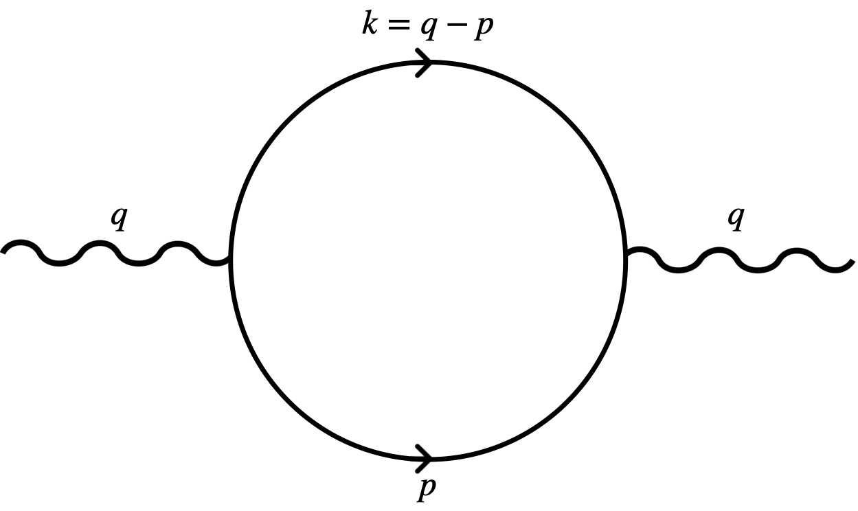
Figure 1: One loop diagram representing the photon polarization tensor with $q$ being the momentum of the photon, and $k$ and $p$ being the momentum of the anti-fermion and fermion, respectively.

III Spectral function and Shear viscosity of fermionic systems from correlation functions

This section demonstrates calculating the shear viscosity of a rotating, hot, and dense fermionic system using the Kubo formalism, which involves computing correlation functions in finite temperature quantum field theory.

We begin with the Kubo formula for shear viscosity

$$\eta=-\frac{1}{10}\displaystyle{\lim_{q_{0}\to 0}}\frac{\rho_{\eta}(q_{0})}{q_{0}}\,,$$ (12)

where $\rho_{\eta}(q)$ is the spectral function of shear viscosity calculated from the two-point correlation function of the shear stress tensor, $\pi^{\mu\nu}=\Delta^{\mu\nu}_{~{}~{}~{}\alpha\beta}\,T^{\alpha\beta}$, and $q_{0}$ is the temporal component of the four-momentum. The expression of $\rho_{\eta}(q)$ is given by

$$\rho_{\eta}(q)=\text{Im}\left[\Pi_{\eta}(q)\right]\,,$$ (13)

where

$$\Pi_{\eta}(q)=i\int d^{4}r~{}e^{iq\cdot r}\big{\langle}\pi^{\mu\nu}(0)\pi_{\mu\nu}(r)\big{\rangle}_{R}\,.$$ (14)

The term $\big{\langle}\mathcal{O}_{1}(x)\mathcal{O}_{2}(y)\big{\rangle}_{R}$ represents the retarded thermal average of the composite field expressions $\mathcal{O}_{1}(x)$ and $\mathcal{O}_{2}(y)$, positioned at spacetime points $x$ and $y$, respectively. The subscript ‘R’ indicates a retarded two-point function.

Equation (13) is formulated in cylindrical coordinates, with the spacetime coordinate at any point denoted as $r=(t,\rho,\phi,z)$. To advance the calculations, it’s necessary to carry out Wick’s contraction of fields, as follows

$$\wick{\c{\psi}(0)\c{\ovpsi}(r)}=S(0,r)=\int\frac{d^{4}p}{(2\pi)^{4}}e^{-ip\cdot r}\left(-iS(p)\right)\,,$$ (15)

where $S(0,r)$ and $S(p)$ is the fermion propagator in coordinate and momentum space, respectively. Using Eq. (15), the two-point correlation function of energy-momentum tensors at two spacetime points is calculated as

$$\langle T^{\mu\nu}(x)T^{\alpha\beta}(y)\rangle = -\frac{1}{16}\Big{\langle}\left[\overline{\psi}\widetilde{\gamma}^{\{\mu}(\widetilde{D}^{\nu\}}\psi)-(\widetilde{D}^{\{\mu}\overline{\psi})\widetilde{\gamma}^{\nu\}}\psi\right]_{x}\left[\overline{\psi}\widetilde{\gamma}^{\{\alpha}(\widetilde{D}^{\beta\}}\psi)-(\widetilde{D}^{\{\alpha}\overline{\psi})\widetilde{\gamma}^{\beta\}}\psi\right]_{y}\Big{\rangle}\,,$$ (16)

$$= -\frac{1}{16}\Big{[}\big{[}\wick{\c{2}\overline{\psi}\widetilde{\gamma}^{\{\mu}(\widetilde{D}^{\nu\}}\c{1}\psi)\big{]}_{x}\big{[}\c{1}\overline{\psi}\widetilde{\gamma}^{\{\alpha}(\widetilde{D}^{\beta\}}\c{2}\psi)\big{]}_{y}}-\wick{\big{[}\c{2}\overline{\psi}\widetilde{\gamma}^{\{\mu}(\widetilde{D}^{\nu\}}\c{1}\psi)\big{]}_{x}\big{[}(\widetilde{D}^{\{\alpha}\c{1}\overline{\psi})\widetilde{\gamma}^{\beta\}}\c{2}\psi\Big{]}_{y}}$$

$$-\wick{\big{[}(\widetilde{D}^{\{\mu}\c{2}\overline{\psi})\widetilde{\gamma}^{\nu\}}\c{1}\psi\big{]}_{x}\big{[}\c{1}\overline{\psi}\widetilde{\gamma}^{\{\alpha}(\widetilde{D}^{\beta\}}\c{2}\psi)\big{]}_{y}}+\wick{\big{[}(\widetilde{D}^{\{\mu}\c{2}\overline{\psi})\widetilde{\gamma}^{\nu\}}\c{1}\psi\big{]}_{x}\big{[}(\widetilde{D}^{\{\alpha}\c{1}\overline{\psi})\widetilde{\gamma}^{\beta\}}\c{2}\psi\big{]}_{y}}\Big{]}\,,$$

where $A^{\{\alpha\beta\}}=A^{\alpha\beta}+A^{\beta\alpha}$. In Eq. (16) we have considered the general spacetime points $x$ and $y$, which can be specified for cylindrical coordinates at the points $r$ and $r^{\prime}$, where $r=(t,\rho,\phi,z)$. Here, $t$ is the time, $\rho$ is the cylinder radius, $\phi$ is the azimuthal angle and $z$ is the height of the cylinder. On substituting Eq. (15) in Eq. (16), the general expression for the two-point function of energy-momentum tensors in cylindrical coordinates is

$$\big{\langle}T^{\mu\nu}(0)T^{\alpha\beta}(r)\big{\rangle} = -\frac{1}{16}\Big{[}\operatorname{Tr}\big{\{}\widetilde{\gamma}^{\{\mu}\widetilde{D}^{\nu\}}S(0,r)\widetilde{\gamma}^{\{\alpha}\widetilde{D}^{\beta\}}S(r,0)\big{\}}-\operatorname{Tr}\big{\{}\widetilde{\gamma}^{\{\mu}\widetilde{D}^{\nu\}}\widetilde{D}^{\{\alpha}S(0,r)\widetilde{\gamma}^{\beta\}}S(r,0)\big{\}}$$ (17)

$$-\operatorname{Tr}\big{\{}\widetilde{\gamma}^{\{\mu}S(0,r)\widetilde{\gamma}^{\{\alpha}\widetilde{D}^{\beta\}}\widetilde{D}^{\nu\}}S(r,0)\big{\}}+\operatorname{Tr}\big{\{}\widetilde{\gamma}^{\{\mu}\widetilde{D}^{\{\alpha}S(0,r)\widetilde{\gamma}^{\beta\}}\widetilde{D}^{\nu\}}S(r,0)\big{\}}\Big{]}.$$

Ref. [94] demonstrates that under rotation, the propagator’s translational invariance is compromised due to the rotation axis favoring a specific direction. A parallel phenomenon occurs in the presence of a background magnetic field [90, 91, 92], where the translational invariance of the propagator is disrupted by a phase shift known as the Schwinger phase factor. In our case, considering a very large $\Omega$ around 0.1 GeV, the phase factor effectively vanishes resulting in the propagator’s dependence solely on relative coordinates

$$S(r,r^{\prime})\xrightarrow{\text{Large~{}}\Omega}S(r-r^{\prime}).$$

Such a situation can be anticipated in the early stages of off-central heavy-ion collisions where $\Omega$ is very large. Using Eq. (17) in Eq. (14) and utilizing the translational invariance property of the propagator, $\Pi_{\eta}(q)$ can be calculated as

$$\Pi_{\eta}(q) = i\int d^{4}r~{}e^{iq\cdot r}\big{\langle}\Delta^{\mu\nu\alpha\beta}T_{\alpha\beta}\Delta_{\mu\nu\rho\lambda}T^{\rho\lambda}\big{\rangle}_{R}$$ (18)

$$= \frac{i}{40}\int d^{4}r\int\int\frac{d^{4}k}{(2\pi)^{4}}\frac{d^{4}p}{(2\pi)^{4}}e^{i(q-p-k)\cdot r}\Bigg{[}(k_{z}-p_{z})^{2}\Big{\{}\operatorname{Tr}\big{\{}\widetilde{\gamma}_{1}S(p)\widetilde{\gamma}^{1}S(k)+\widetilde{\gamma}_{3}S(p)\widetilde{\gamma}^{3}S(k)\big{\}}\Big{\}}$$

$$+\frac{1}{3}\,\Bigg{\{}-2\operatorname{Tr}\Big{\{}\widetilde{\gamma}^{0}\Big{(}p_{0}+\frac{\Omega\Sigma_{3}}{2}\Big{)}S(p)\widetilde{\gamma}^{0}\Big{(}k_{0}+\frac{\Omega\Sigma_{3}}{2}\Big{)}S(k)\Big{\}}+\operatorname{Tr}\Big{\{}\widetilde{\gamma}^{0}\Big{(}p_{0}+\frac{\Omega\Sigma_{3}}{2}\Big{)}^{2}S(p)\widetilde{\gamma}_{0}S(k)\Big{\}}$$

$$+\operatorname{Tr}\Big{\{}\widetilde{\gamma}^{0}S(p)\widetilde{\gamma}_{0}\Big{(}k_{0}+\frac{\Omega\Sigma_{3}}{2}\Big{)}^{2}S(k)\Big{\}}+\operatorname{Tr}\Big{\{}\widetilde{\gamma}^{0}\Big{(}p_{0}+\frac{\Omega\Sigma_{3}}{2}\Big{)}S(p)\widetilde{\gamma}^{3}k_{z}S(k)\Big{\}}$$

$$+\operatorname{Tr}\Big{\{}\widetilde{\gamma}^{0}p_{z}\Big{(}p_{0}+\frac{\Omega\Sigma_{3}}{2}\Big{)}S(p)\widetilde{\gamma}_{3}S(k)\Big{\}}-\operatorname{Tr}\Big{\{}\widetilde{\gamma}_{0}S(p)\widetilde{\gamma}^{3}k_{z}\Big{(}k_{0}+\frac{\Omega\Sigma_{3}}{2}\Big{)}S(k)\Big{\}}$$

$$+\operatorname{Tr}\Big{\{}\widetilde{\gamma}_{0}p_{z}S(p)\widetilde{\gamma}_{3}\Big{(}k_{0}+\frac{\Omega\Sigma_{3}}{2}\Big{)}S(k)\Big{\}}+\operatorname{Tr}\Big{\{}\widetilde{\gamma}^{3}p_{z}S(p)\widetilde{\gamma}^{0}\Big{(}k_{0}+\frac{\Omega\Sigma_{3}}{2}\Big{)}S(k)\Big{\}}$$

$$-\operatorname{Tr}\Big{\{}\widetilde{\gamma}^{3}p_{z}\Big{(}p_{0}+\frac{\Omega\Sigma_{3}}{2}\Big{)}S(p)\widetilde{\gamma}_{0}S(k)\Big{\}}-\operatorname{Tr}\Big{\{}\widetilde{\gamma}_{3}S(p)\widetilde{\gamma}_{0}k_{z}\Big{(}k_{0}+\frac{\Omega\Sigma_{3}}{2}\Big{)}S(k)\Big{\}}$$

$$-\operatorname{Tr}\Big{\{}\widetilde{\gamma}_{3}\Big{(}p_{0}+\frac{\Omega\Sigma_{3}}{2}\Big{)}S(p)\widetilde{\gamma}_{0}k_{z}S(k)\Big{\}}-(p_{z}+k_{z})^{2}\operatorname{Tr}\Big{\{}\widetilde{\gamma}^{3}S(p)\widetilde{\gamma}^{3}S(k)\Big{\}}$$

$$+\operatorname{Tr}\Big{\{}\widetilde{\gamma}^{0}\Big{(}p_{0}+\frac{\Omega\Sigma_{3}}{2}\Big{)}S(p)\widetilde{\gamma}^{0}\Big{(}k_{0}+\frac{\Omega\Sigma_{3}}{2}\Big{)}S(k)\Big{\}}-\operatorname{Tr}\Big{\{}\widetilde{\gamma}^{0}\Big{(}p_{0}+\frac{\Omega\Sigma_{3}}{2}\Big{)}^{2}S(p)\widetilde{\gamma}^{0}S(k)\Big{\}}$$

$$-\operatorname{Tr}\Big{\{}\widetilde{\gamma}^{0}S(p)\widetilde{\gamma}^{0}\Big{(}k_{0}+\frac{\Omega\Sigma_{3}}{2}\Big{)}^{2}S(k)\Big{\}}-\operatorname{Tr}\Big{\{}\widetilde{\gamma}^{3}p_{z}S(p)\widetilde{\gamma}^{0}\Big{(}k_{0}+\frac{\Omega\Sigma_{3}}{2}\Big{)}S(k)\Big{\}}$$

$$+\operatorname{Tr}\Big{\{}\widetilde{\gamma}^{3}p_{z}\Big{(}p_{0}+\frac{\Omega\Sigma_{3}}{2}\Big{)}S(p)\widetilde{\gamma}_{0}S(k)\Big{\}}-\operatorname{Tr}\Big{\{}\widetilde{\gamma}_{3}S(p)\widetilde{\gamma}^{0}k_{z}\Big{(}k_{0}+\frac{\Omega\Sigma_{3}}{2}\Big{)}S(k)\Big{\}}$$

$$+\operatorname{Tr}\Big{\{}\widetilde{\gamma}_{3}\Big{(}p_{0}+\frac{\Omega\Sigma_{3}}{2}\Big{)}S(p)\widetilde{\gamma}_{0}k_{z}S(k)\Big{\}}-\operatorname{Tr}\Big{\{}\widetilde{\gamma}_{0}\Big{(}p_{0}+\frac{\Omega\Sigma_{3}}{2}\Big{)}^{2}S(p)\widetilde{\gamma}_{0}S(k)\Big{\}}$$

$$-\operatorname{Tr}\Big{\{}\widetilde{\gamma}_{0}S(p)\widetilde{\gamma}^{0}\Big{(}k_{0}+\frac{\Omega\Sigma_{3}}{2}\Big{)}^{2}S(k)\Big{\}}+\operatorname{Tr}\Big{\{}\widetilde{\gamma}_{0}\Big{(}p_{0}+\frac{\Omega\Sigma_{3}}{2}\Big{)}S(p)\widetilde{\gamma}_{0}\Big{(}k_{0}+\frac{\Omega\Sigma_{3}}{2}\Big{)}S(k)\Big{\}}$$

$$+\operatorname{Tr}\Big{\{}\widetilde{\gamma}_{0}\Big{(}p_{0}+\frac{\Omega\Sigma_{3}}{2}\Big{)}S(p)\widetilde{\gamma}^{3}k_{z}S(k)\Big{\}}+\operatorname{Tr}\Big{\{}\widetilde{\gamma}_{0}\Big{(}p_{0}+\frac{\Omega\Sigma_{3}}{2}\Big{)}p_{z}S(p)\widetilde{\gamma}_{3}S(k)\Big{\}}$$

$$-\operatorname{Tr}\Big{\{}\widetilde{\gamma}_{0}S(p)\widetilde{\gamma}^{3}k_{z}\Big{(}k_{0}+\frac{\Omega\Sigma_{3}}{2}\Big{)}S(k)\Big{\}}-\operatorname{Tr}\Big{\{}\widetilde{\gamma}_{0}p_{z}S(p)\widetilde{\gamma}_{3}\Big{(}k_{0}+\frac{\Omega\Sigma_{3}}{2}\Big{)}S(k)\Big{\}}$$

$$-\operatorname{Tr}\Big{\{}\widetilde{\gamma}_{0}\Big{(}p_{0}+\frac{\Omega\Sigma_{3}}{2}\Big{)}S(p)\widetilde{\gamma}^{0}\Big{(}k_{0}+\frac{\Omega\Sigma_{3}}{2}\Big{)}S(k)\Big{\}}+\operatorname{Tr}\Big{\{}\widetilde{\gamma}_{0}\Big{(}p_{0}+\frac{\Omega\Sigma_{3}}{2}\Big{)}^{2}S(p)\widetilde{\gamma}^{0}S(k)\Big{\}}$$

$$-\operatorname{Tr}\Big{\{}\widetilde{\gamma}_{0}S(p)\widetilde{\gamma}^{0}\Big{(}k_{0}+\frac{\Omega\Sigma_{3}}{2}\Big{)}^{2}S(k)\Big{\}}\Bigg{\}}\Bigg{]}\,.$$

Upon integrating over $d^{4}r$ and $d^{4}k$, we obtain a delta function $(2\pi)^{4}\delta(q-p-k)$, ensuring momentum conservation at the vertex. This conservation sets specific relationships between $p$, $k$, and $q$: $k_{0}=q_{0}-p_{0}$, $k_{z}=q_{z}-p_{z}$, and $k_{\perp}=q_{\perp}-p_{\perp}$, consistent with the one-loop diagram for photon polarization shown in Fig. 1. The spectral function, Eq. (13), is then computed using Eq. (18) and is expressed as

$$\rho_{\eta}(q) = \text{Im~{}}i\int d^{4}r~{}e^{iq\cdot r}\big{\langle}\Delta^{\mu\nu\alpha\beta}T_{\alpha\beta}\Delta_{\mu\nu\rho\lambda}T^{\rho\lambda}\big{\rangle}_{R}$$ (19)

$$= \text{Im}\frac{i}{40}\int d^{4}r\int\frac{d^{4}p}{(2\pi)^{4}}\Bigg{[}(q_{z}-2p_{z})^{2}\Big{\{}\operatorname{Tr}\big{\{}\widetilde{\gamma}_{1}S(p)\widetilde{\gamma}^{1}S(q-p)+\widetilde{\gamma}_{3}S(p)\widetilde{\gamma}^{3}S(q-p)\big{\}}\Big{\}}$$

$$+\frac{1}{3}\Bigg{\{}-2\operatorname{Tr}\Big{\{}\widetilde{\gamma}^{0}\Big{(}p_{0}+\frac{\Omega\Sigma_{3}}{2}\Big{)}S(p)\widetilde{\gamma}^{0}\Big{(}q_{0}-p_{0}+\frac{\Omega\Sigma_{3}}{2}\Big{)}S(q-p)\Big{\}}+\operatorname{Tr}\Big{\{}\widetilde{\gamma}^{0}\Big{(}p_{0}+\frac{\Omega\Sigma_{3}}{2}\Big{)}^{2}S(p)\widetilde{\gamma}_{0}S(q-p)\Big{\}}$$

$$+\operatorname{Tr}\Big{\{}\widetilde{\gamma}^{0}S(p)\widetilde{\gamma}_{0}\Big{(}q_{0}-p_{0}+\frac{\Omega\Sigma_{3}}{2}\Big{)}^{2}S(q-p)\Big{\}}+\operatorname{Tr}\Big{\{}\widetilde{\gamma}^{0}\Big{(}p_{0}+\frac{\Omega\Sigma_{3}}{2}\Big{)}S(p)\widetilde{\gamma}^{3}k_{z}S(q-p)\Big{\}}$$

$$+\operatorname{Tr}\Big{\{}\widetilde{\gamma}^{0}p_{z}\Big{(}p_{0}+\frac{\Omega\Sigma_{3}}{2}\Big{)}S(p)\widetilde{\gamma}_{3}S(q-p)\Big{\}}-\operatorname{Tr}\Big{\{}\widetilde{\gamma}_{0}S(p)\widetilde{\gamma}^{3}(q_{z}-p_{z})\Big{(}q_{0}-p_{0}+\frac{\Omega\Sigma_{3}}{2}\Big{)}S(q-p)\Big{\}}$$

$$+\operatorname{Tr}\Big{\{}\widetilde{\gamma}_{0}p_{z}S(p)\widetilde{\gamma}_{3}\Big{(}q_{0}-p_{0}+\frac{\Omega\Sigma_{3}}{2}\Big{)}S(q-p)\Big{\}}+\operatorname{Tr}\Big{\{}\widetilde{\gamma}^{3}p_{z}S(p)\widetilde{\gamma}^{0}\Big{(}q_{0}-p_{0}+\frac{\Omega\Sigma_{3}}{2}\Big{)}S(q-p)\Big{\}}$$

$$-\operatorname{Tr}\Big{\{}\widetilde{\gamma}^{3}p_{z}\Big{(}p_{0}+\frac{\Omega\Sigma_{3}}{2}\Big{)}S(p)\widetilde{\gamma}_{0}S(q-p)\Big{\}}-\operatorname{Tr}\Big{\{}\widetilde{\gamma}_{3}S(p)\widetilde{\gamma}_{0}(q_{z}-p_{z})\Big{(}q_{0}-p_{0}+\frac{\Omega\Sigma_{3}}{2}\Big{)}S(q-p)\Big{\}}$$

$$-\operatorname{Tr}\Big{\{}\widetilde{\gamma}_{3}\Big{(}p_{0}+\frac{\Omega\Sigma_{3}}{2}\Big{)}S(p)\widetilde{\gamma}_{0}(q_{z}-p_{z})S(q-p)\Big{\}}-q_{z}^{2}\operatorname{Tr}\Big{\{}\widetilde{\gamma}^{3}S(p)\widetilde{\gamma}^{3}S(q-z)\Big{\}}$$

$$+\operatorname{Tr}\Big{\{}\widetilde{\gamma}^{0}\Big{(}p_{0}+\frac{\Omega\Sigma_{3}}{2}\Big{)}S(p)\widetilde{\gamma}^{0}\Big{(}q_{0}-p_{0}+\frac{\Omega\Sigma_{3}}{2}\Big{)}S(q-p)\Big{\}}-\operatorname{Tr}\Big{\{}\widetilde{\gamma}^{0}\Big{(}p_{0}+\frac{\Omega\Sigma_{3}}{2}\Big{)}^{2}S(p)\widetilde{\gamma}^{0}S(q-p)\Big{\}}$$

$$-\operatorname{Tr}\Big{\{}\widetilde{\gamma}^{0}S(p)\widetilde{\gamma}^{0}\Big{(}q_{0}-p_{0}+\frac{\Omega\Sigma_{3}}{2}\Big{)}^{2}S(q-p)\Big{\}}-\operatorname{Tr}\Big{\{}\widetilde{\gamma}^{3}p_{z}S(p)\widetilde{\gamma}^{0}\Big{(}q_{0}-p_{0}+\frac{\Omega\Sigma_{3}}{2}\Big{)}S(q-p)\Big{\}}$$

$$+\operatorname{Tr}\Big{\{}\widetilde{\gamma}^{3}p_{z}\Big{(}p_{0}+\frac{\Omega\Sigma_{3}}{2}\Big{)}S(p)\widetilde{\gamma}_{0}S(q-p)\Big{\}}-\operatorname{Tr}\Big{\{}\widetilde{\gamma}_{3}S(p)\widetilde{\gamma}^{0}(q_{z}-p_{z})\Big{(}q_{0}-p_{0}+\frac{\Omega\Sigma_{3}}{2}\Big{)}S(q-p)\Big{\}}$$

$$+\operatorname{Tr}\Big{\{}\widetilde{\gamma}_{3}\Big{(}p_{0}+\frac{\Omega\Sigma_{3}}{2}\Big{)}S(p)\widetilde{\gamma}_{0}(q_{z}-p_{z})S(q-p)\Big{\}}-\operatorname{Tr}\Big{\{}\widetilde{\gamma}_{0}\Big{(}p_{0}+\frac{\Omega\Sigma_{3}}{2}\Big{)}^{2}S(p)\widetilde{\gamma}_{0}S(q-p)\Big{\}}$$

$$-\operatorname{Tr}\Big{\{}\widetilde{\gamma}_{0}S(p)\widetilde{\gamma}^{0}\Big{(}q_{0}-p_{0}+\frac{\Omega\Sigma_{3}}{2}\Big{)}^{2}S(q-p)\Big{\}}+\operatorname{Tr}\Big{\{}\widetilde{\gamma}_{0}\Big{(}p_{0}+\frac{\Omega\Sigma_{3}}{2}\Big{)}S(p)\widetilde{\gamma}_{0}\Big{(}q_{0}-p_{0}+\frac{\Omega\Sigma_{3}}{2}\Big{)}S(q-p)\Big{\}}$$

$$+\operatorname{Tr}\Big{\{}\widetilde{\gamma}_{0}\Big{(}p_{0}+\frac{\Omega\Sigma_{3}}{2}\Big{)}S(p)\widetilde{\gamma}^{3}(q_{z}-p_{z})S(q-p)\Big{\}}+\operatorname{Tr}\Big{\{}\widetilde{\gamma}_{0}\Big{(}p_{0}+\frac{\Omega\Sigma_{3}}{2}\Big{)}p_{z}S(p)\widetilde{\gamma}_{3}S(q-p)\Big{\}}$$

$$-\operatorname{Tr}\Big{\{}\widetilde{\gamma}_{0}S(p)\widetilde{\gamma}^{3}(q_{z}-p_{z})\Big{(}q_{0}-p_{0}+\frac{\Omega\Sigma_{3}}{2}\Big{)}S(q-p)\Big{\}}-\operatorname{Tr}\Big{\{}\widetilde{\gamma}_{0}p_{z}S(p)\widetilde{\gamma}_{3}\Big{(}q_{0}-p_{0}+\frac{\Omega\Sigma_{3}}{2}\Big{)}S(q-p)\Big{\}}$$

$$-\operatorname{Tr}\Big{\{}\widetilde{\gamma}_{0}\Big{(}p_{0}+\frac{\Omega\Sigma_{3}}{2}\Big{)}S(p)\widetilde{\gamma}^{0}\Big{(}q_{0}-p_{0}+\frac{\Omega\Sigma_{3}}{2}\Big{)}S(q-p)\Big{\}}+\operatorname{Tr}\Big{\{}\widetilde{\gamma}_{0}\Big{(}p_{0}+\frac{\Omega\Sigma_{3}}{2}\Big{)}^{2}S(p)\widetilde{\gamma}^{0}S(q-p)\Big{\}}$$

$$-\operatorname{Tr}\Big{\{}\widetilde{\gamma}_{0}S(p)\widetilde{\gamma}^{0}\Big{(}q_{0}-p_{0}+\frac{\Omega\Sigma_{3}}{2}\Big{)}^{2}S(q-p)\Big{\}}\Bigg{\}}\Bigg{]}\,.$$

To execute the integration in Eq. (19), we will carry out the Matsubara frequency summation, considering finite angular velocity and chemical potential. In the following we present details the Matsubara frequency summation process applied to compute the spectral function of energy-momentum tensors. At finite temperature

$$p_{0} \to i\widetilde{\omega}_{N}=(2N+1)\pi T\,,\quad q_{0}\to i\nu_{N}=2\pi NT\,,$$

$$\int\frac{d^{4}p}{(2\pi)^{4}} \equiv \sum\!\!\!\!\!\!\!\!\!\int\limits_{\{P\}}=iT\sum_{N=-\infty}^{+\infty}\int\frac{d^{3}p}{(2\pi)^{3}},$$ (20)

where $N\in\mathbb{Z}$, and $p_{0}$ and $q_{0}$ are the temporal components of the four-momentum of the fermion and boson, respectively, in the photon polarization. In one-loop calculations of spectral functions, the fermion propagator under rotation, Eq. (11), leads to fermionic Matsubara frequency summations of the type

$$(a) T\sum_{\{p_{N}\}}\frac{1}{\big{[}i\widetilde{\omega}_{N}+\frac{\Omega}{2}+\mu\big{]}^{2}-\vec{p}^{2}-m^{2}}\frac{1}{\big{[}i\nu_{N}-i\widetilde{\omega}_{N}+\frac{\Omega}{2}-\mu\big{]}^{2}-\vec{k}^{2}-m^{2}}\,,$$ (21)

$$(b) T\sum_{\{p_{N}\}}\frac{1}{\big{[}i\widetilde{\omega}_{N}+\frac{\Omega}{2}+\mu\big{]}^{2}-\vec{p}^{2}-m^{2}}\frac{1}{\big{[}i\nu_{N}-i\widetilde{\omega}_{N}-\frac{\Omega}{2}-\mu\big{]}^{2}-\vec{k}^{2}-m^{2}}\,,$$ (22)

$$(c) T\sum_{\{p_{N}\}}\frac{1}{\big{[}i\widetilde{\omega}_{N}-\frac{\Omega}{2}+\mu\big{]}^{2}-\vec{p}^{2}-m^{2}}\frac{1}{\big{[}i\nu_{N}-i\widetilde{\omega}_{N}+\frac{\Omega}{2}-\mu\big{]}^{2}-\vec{k}^{2}-m^{2}}\,,$$ (23)

$$(d) T\sum_{\{p_{N}\}}\frac{1}{\big{[}i\widetilde{\omega}_{N}-\frac{\Omega}{2}+\mu\big{]}^{2}-\vec{p}^{2}-m^{2}}\frac{1}{\big{[}i\nu_{N}-i\widetilde{\omega}_{N}-\frac{\Omega}{2}-\mu\big{]}^{2}-\vec{k}^{2}-m^{2}}\,.$$ (24)

Utilizing the Saclay method for evaluating Matsubara frequency sums [98], we derive the results for the frequency summations, Eqs. (21)-(24), expressed as

$$(a)\quad T\sum_{\{p_{N}\}}\frac{1}{\big{[}i\widetilde{\omega}_{N}+\frac{\Omega}{2}+\mu\big{]}^{2}-\vec{p}^{2}-m^{2}}\frac{1}{\big{[}i\nu_{N}-i\widetilde{\omega}_{N}+\frac{\Omega}{2}-\mu\big{]}^{2}-\vec{k}^{2}-m^{2}}$$

$$=\frac{1}{4E_{p}E_{k}}\Bigg{\{}\frac{n_{F}(E_{p}+\mu+\Omega/2)+n_{F}(E_{k}-\mu+\Omega/2)-1}{q_{0}-E_{p}-E_{k}}+\frac{n_{F}(E_{k}+\mu+\Omega/2)-n_{F}(E_{p}+\mu+\Omega/2)}{q_{0}+E_{k}-E_{p}}$$

$$+\frac{n_{F}(E_{p}-\mu-\Omega/2)-n_{F}(E_{k}-\mu-\Omega/2)}{q_{0}+E_{p}-E_{k}}+\frac{1-n_{F}(E_{p}-\mu-\Omega/2)-n_{F}(E_{k}+\mu-\Omega/2)}{q_{0}+E_{k}+E_{p}}\Bigg{\}}\,,$$ (25)

$$(b)\quad T\sum_{\{p_{N}\}}\frac{1}{\big{[}i\widetilde{\omega}_{N}+\frac{\Omega}{2}+\mu\big{]}^{2}-\vec{p}^{2}-m^{2}}\frac{1}{\big{[}i\nu_{N}-i\widetilde{\omega}_{N}-\frac{\Omega}{2}-\mu\big{]}^{2}-\vec{k}^{2}-m^{2}}$$

$$=\frac{1}{4E_{p}E_{k}}\Bigg{\{}\frac{n_{F}(E_{p}+\mu+\Omega/2)+n_{F}(E_{k}-\mu-\Omega/2)-1}{q_{0}-E_{p}-E_{k}}+\frac{n_{F}(E_{k}+\mu+\Omega/2)-n_{F}(E_{p}+\mu+\Omega/2)}{q_{0}+E_{k}-E_{p}}$$

$$+\frac{n_{F}(E_{p}-\mu-\Omega/2)-n_{F}(E_{k}-\mu-\Omega/2)}{q_{0}+E_{p}-E_{k}}+\frac{1-n_{F}(E_{p}-\mu-\Omega/2)-n_{F}(E_{k}+\mu+\Omega/2)}{q_{0}+E_{k}+E_{p}}\Bigg{\}}\,,$$ (26)

$$(c)\quad T\sum_{\{p_{N}\}}\frac{1}{\big{[}i\widetilde{\omega}_{N}-\frac{\Omega}{2}+\mu\big{]}^{2}-\vec{p}^{2}-m^{2}}\frac{1}{\big{[}i\nu_{N}-i\widetilde{\omega}_{N}+\frac{\Omega}{2}-\mu\big{]}^{2}-\vec{k}^{2}-m^{2}}$$

$$=\frac{1}{4E_{p}E_{k}}\Bigg{\{}\frac{n_{F}(E_{p}+\mu-\Omega/2)+n_{F}(E_{k}-\mu+\Omega/2)-1}{q_{0}-E_{p}-E_{k}}+\frac{n_{F}(E_{k}+\mu-\Omega/2)-n_{F}(E_{k}+\mu-\Omega/2)}{q_{0}+E_{k}-E_{p}}$$

$$+\frac{n_{F}(E_{p}-\mu+\Omega/2)-n_{F}(E_{k}-\mu+\Omega/2)}{q_{0}+E_{p}-E_{k}}+\frac{1-n_{F}(E_{p}-\mu+\Omega/2)-n_{F}(E_{k}+\mu-\Omega/2)}{q_{0}+E_{k}+E_{p}}\Bigg{\}}\,,$$ (27)

$$(d)\quad T\sum_{\{p_{N}\}}\frac{1}{\big{[}i\widetilde{\omega}_{N}-\frac{\Omega}{2}+\mu\big{]}^{2}-\vec{p}^{2}-m^{2}}\frac{1}{\big{[}i\nu_{N}-i\widetilde{\omega}_{N}-\frac{\Omega}{2}-\mu\big{]}^{2}-\vec{k}^{2}-m^{2}}$$

$$=\frac{1}{4E_{p}E_{k}}\Bigg{\{}\frac{n_{F}(E_{p}+\mu-\Omega/2)+n_{F}(E_{k}-\mu-\Omega/2)-1}{q_{0}-E_{p}-E_{k}}+\frac{n_{F}(E_{k}+\mu-\Omega/2)-n_{F}(E_{k}+\mu-\Omega/2)}{q_{0}+E_{k}-E_{p}}$$

$$+\frac{n_{F}(E_{p}-\mu+\Omega/2)-n_{F}(E_{k}-\mu+\Omega/2)}{q_{0}+E_{p}-E_{k}}+\frac{1-n_{F}(E_{p}-\mu+\Omega/2)-n_{F}(E_{k}+\mu-\Omega/2)}{q_{0}+E_{k}+E_{p}}\Bigg{\}}.$$ (28)

In the above equations, there are four different combinations of $q_{0}$, $E_{k}$, and $E_{p}$ in the denominators: $q_{0}\pm E_{k}\pm E_{p}$ and $q_{0}\mp E_{k}\pm E_{p}$, which can be interpreted as energy limit values from the upper half plane. By transforming $\nu_{N}\to-i(q_{0}+i0^{+})$ through the analytic continuation of discrete Matsubara frequencies to continuous energies, we can extract the imaginary part as needed in Eq. (19), utilizing the relation

$$\frac{1}{\Delta\pm i0^{+}}=\mathbb{P}\left(\frac{1}{\Delta}\right)\mp i\pi\delta(\Delta).$$ (29)

where $\mathbb{P}$ is the principal part of the function. Employing Eq. (29), $\rho_{\eta}(q)$ is given as

$$\rho_{\eta}(q) = -\pi\int\frac{d^{3}p}{(2\pi)^{3}}\Big{(}\frac{\mathcal{C}(p_{\perp},p_{z},p_{0},q_{\perp},q_{z},q_{0})}{4E_{p}E_{q-p}}\Big{)}\Bigg{[}\Big{\{}n_{F}(E_{q-p}+\bar{\mu})-n_{F}(E_{p}+\bar{\mu})\Big{\}}\Big{\{}\delta(q_{0}+E_{q-p}-E_{p})\Big{\}}$$ (30)

$$+\,\Big{\{}n_{F}(E_{p}-\bar{\mu})-n_{F}(E_{q-p}-\bar{\mu})\Big{\}}\Big{\{}\delta(q_{0}+E_{p}-E_{q-p})\Big{\}}$$

$$+\,\Big{\{}n_{F}(E_{q-p}+\bar{\mu})+n_{F}(E_{p}-\bar{\mu})-1\Big{\}}\Big{\{}\delta(q_{0}-E_{q-p}-E_{p})\Big{\}}$$

$$+\,\Big{\{}n_{F}(E_{q-p}-\bar{\mu})+n_{F}(E_{p}+\bar{\mu})-1\Big{\}}\Big{\{}\delta(q_{0}+E_{q-p}+E_{p})\Big{\}}\Bigg{]}$$

$$-\,\pi\int\frac{d^{3}p}{(2\pi)^{3}}\Big{(}\frac{\mathcal{D}(p_{\perp},p_{z},p_{0},q_{\perp},q_{z},q_{0})}{4E_{p}E_{q-p}}\Big{)}\Bigg{[}\Big{\{}n_{F}(E_{q-p}+\widetilde{\mu})-n_{F}(E_{p}+\widetilde{\mu})\Big{\}}\Big{\{}\delta(q_{0}+E_{q-p}-E_{p})\Big{\}}$$

$$+\,\Big{\{}n_{F}(E_{p}-\widetilde{\mu})-n_{F}(E_{q-p}-\widetilde{\mu})\Big{\}}\Big{\{}\delta(q_{0}+E_{p}-E_{q-p})\Big{\}}$$

$$+\,\Big{\{}n_{F}(E_{q-p}+\widetilde{\mu})+n_{F}(E_{p}-\widetilde{\mu})-1\Big{\}}\Big{\{}\delta(q_{0}-E_{q-p}-E_{p})\Big{\}}$$

$$+\,\Big{\{}n_{F}(E_{q-p}-\widetilde{\mu})+n_{F}(E_{p}+\widetilde{\mu})-1\Big{\}}\Big{\{}\delta(q_{0}+E_{q-p}+E_{p})\Big{\}}\Bigg{]}\,,$$

where $\bar{\mu}=\mu+\frac{\Omega}{2}\text{~{}~{}and~{}~{}}\widetilde{\mu}=\mu-\frac{\Omega}{2}$ are the combinations of chemical potential and angular velocity. $\mathcal{C}(p_{\perp},p_{z},p_{0},q_{\perp},q_{z},q_{0})$ and $\mathcal{D}(p_{\perp},p_{z},p_{0},q_{\perp},q_{z},q_{0})$ are functions expressed as

$$\mathcal{C}(p_{\perp},p_{z},p_{0},q_{\perp},q_{z},q_{0})=-\frac{1}{480}\Big{\{}2(p_{z}-q_{z})\big{(}q_{0}-p_{0}+8p_{z}-2p_{0}+\Omega\big{)}+8(q_{z}-p_{z})^{2}+3(q_{0}-p_{0})\Omega$$

$$+\,p_{z}\big{(}8p_{z}-2p_{0}+\Omega\big{)}\big{]}\big{[}(q_{z}-p_{z})\big{(}4p_{z}+4p_{0}-2\Omega\big{)}-4(q_{\perp}-p_{\perp})p_{\perp}+\big{(}2q_{0}-2p_{0}-\Omega\big{)}\big{(}2p_{z}+2p_{0}-\Omega\big{)}\big{]}$$

$$+\frac{1}{10}\big{[}p_{z}\big{(}q_{z}-2p_{z}\big{)}\big{]}\big{[}(q_{z}-p_{z})\big{(}4p_{z}-4p_{0}-2\Omega\big{)}-4(q_{\perp}-p_{\perp})p_{\perp}+\big{(}2q_{0}-2p_{0}-\Omega\big{)}\big{(}2p_{z}+2p_{0}+\Omega\big{)}\Big{\}}\,,$$ (31)

$$\mathcal{D}(p_{\perp},p_{z},p_{0},q_{\perp},q_{z},q_{0})=-\frac{1}{480}\Big{\{}2(p_{z}-q_{z})\big{(}q_{0}-p_{0}+8p_{z}+2p_{0}+\Omega\big{)}+8(q_{z}-p_{z})^{2}+3(q_{0}-p_{0})\Omega$$

$$+\,p_{z}\big{(}8p_{z}+2p_{0}+\Omega\big{)}\big{]}\big{[}-k_{z}\big{(}-4p_{z}+4p_{0}+2\Omega\big{)}-4(q_{\perp}-p_{\perp})p_{\perp}+\big{(}2q_{0}-2p_{0}+\Omega\big{)}\big{(}-2p_{z}+2p_{0}+\Omega\big{)}\big{]}$$

$$+\frac{1}{10}\big{[}p_{z}\big{(}q_{z}-2p_{z}\big{)}\big{]}\big{[}(q_{z}-p_{z})\big{(}4p_{z}+4p_{0}+2\Omega\big{)}-4(q_{\perp}-p_{\perp})p_{\perp}+\big{(}2q_{0}-2p_{0}+\Omega\big{)}\big{(}-2p_{z}+2p_{0}+\Omega\big{)}\Big{\}}.$$ (32)

It’s important to note that $\rho_{\eta}(q)$, as determined in Eq. (30) through analytic continuation and the cut of a Euclidean correlator, represents real scatterings of on-shell particles. These scatterings are kinematically allowed and their distribution is described by the Fermi-Dirac distribution function. More precisely, the imaginary parts are associated with real particle scatterings, information about which is conveyed by the delta functions in Eq. (30). The delta functions $\delta(q_{0}\pm E_{p}\mp E_{k})$, known as Landau cuts, and $\delta(q_{0}\pm E_{p}\pm E_{k})$, known as unitary cuts. Landau cuts only occur at finite temperature, while unitary cuts, also present due to vacuum contributions, don’t contribute to transport coefficient calculations and are thus omitted here [99]. From Eq. (12), the shear viscosity, as calculated using Eq. (30), is

$$\eta = \displaystyle{\lim_{q_{0}\to 0,\,\vec{q}=\vec{0}}}\text{Im}\Bigg{[}-\pi\int\frac{d^{3}p}{(2\pi)^{3}}\frac{\mathcal{C}(p_{\perp},p_{z},p_{0},q_{\perp},q_{z},q_{0})}{4E_{q-p}E_{p}}$$ (33)

$$\displaystyle{\lim_{\Gamma\to 0}}\Bigg{\{}\frac{\big{(}n_{F}(E_{q-p}+\bar{\mu})-n_{F}(E_{p}+\bar{\mu})\big{)}/q_{0}}{q_{0}+E_{q-p}-E_{p}+i\Gamma}+\frac{\big{(}n_{F}(E_{q-p}-\bar{\mu})-n_{F}(E_{p}-\bar{\mu})\big{)}/q_{0}}{q_{0}+E_{p}-E_{q-p}+i\Gamma}\Bigg{\}}\Bigg{]}$$

$$+ \displaystyle{\lim_{q_{0}\to 0,\,\vec{q}=\vec{0}}}\text{Im}\Bigg{[}-\pi\int\frac{d^{3}p}{(2\pi)^{3}}\frac{\mathcal{D}(p_{\perp},p_{z},p_{0},q_{\perp},q_{z},q_{0})}{4E_{q-p}E_{p}}$$

$$\displaystyle{\lim_{\Gamma\to 0}}\Bigg{\{}\frac{\big{(}n_{F}(E_{q-p}+\widetilde{\mu})-n_{F}(E_{p}+\widetilde{\mu})\big{)}/q_{0}}{q_{0}+E_{q-p}-E_{p}+i\Gamma}+\frac{\big{(}n_{F}(E_{q-p}-\widetilde{\mu})-n_{F}(E_{p}-\widetilde{\mu})\big{)}/q_{0}}{q_{0}+E_{p}-E_{q-p}+i\Gamma}\Bigg{\}}\Bigg{]}\,.$$

In the equation, we use the representation $\delta(x)=-(1/\pi)\lim_{\Gamma\to 0}\frac{1}{x+i\Gamma}$, where $\Gamma$ is the thermal width of the medium. This width arises from interactions within the medium at finite temperature, with high system temperatures effectively generating interactions (i.e., a finite $\Gamma$). Notably, $\Gamma$ is essentially the inverse of the relaxation time $\tau$, i.e., $\Gamma=1/\tau$ [99]. In this work, $\Gamma$ is introduced via the Breit-Wigner form, and a similar approach can be applied by including a half-width $i\Gamma/2$ [100] in the momentum space propagators. This involves considering the expression for the inverse of the retarded momentum space propagator $G^{-1}_{\text{R}}(p)$ with the complex self-energy $\Sigma_{\text{R}}(p)$: $G_{\text{R}}^{-1}(p)=p^{2}-m_{0}^{2}-\text{Re}\Sigma_{\text{R}}(p)-i\text{Im}\Sigma_{\text{R}}(p)\sim(p_{0}+i\gamma(p))^{2}-E_{p}^{2}$, where $\gamma=-\frac{1}{2p_{0}}\text{Im}\Sigma_{\text{R}}(p)=\frac{\Gamma}{2}$. This indicates that $\Gamma$ is inherent in the theory’s propagator. In our calculations, we use a specific form of the $\delta(x)$ function to incorporate this information. $\Gamma$ can be calculated using an interacting Lagrangian and thermal field theory techniques [98, 100]. At the $\vec{q}=\vec{0},\,q_{0}\to 0$ limit, $\eta$ appears indeterminate (0/0 form), which is unphysical. To address this, we apply L’Hospital’s rule. In a free theory where interaction is absent ($\Gamma\to 0$), shear viscosity becomes infinite. Thus, a finite $\Gamma$ is necessary to yield a non-divergent shear viscosity. The final expression for $\eta(T,\mu,\Omega)$ is then

$$\eta(T,\mu,\Omega)=\frac{1}{240}\int\frac{d^{3}p}{(2\pi)^{3}}\left(\frac{1}{4E_{p}^{2}\Gamma T}\right)$$ (34)

$$\Bigg{\{}\Big{\{}160p_{z}^{4}+4p_{\perp}^{2}\Omega^{2}+\big{(}\Omega-E_{p}-3p_{z}\big{)}\Omega^{3}+8p_{\perp}^{2}p_{z}\big{(}\Omega-4E_{p}\big{)}+32p_{z}^{3}\big{(}\Omega+5E_{p}\big{)}-8p_{z}^{2}\Omega\big{(}2E_{p}+3\Omega\big{)}\Big{\}}\mathcal{N}_{\pm\mu,\mp\Omega/2}$$

$$+\Big{\{}160p_{z}^{4}+4p_{\perp}^{2}\Omega^{2}+\big{(}\Omega-E_{p}-3p_{z}\big{)}\Omega^{3}+8p_{\perp}^{2}p_{z}\big{(}\Omega-4E_{p}\big{)}+32p_{z}^{3}\big{(}\Omega-5E_{p}\big{)}-8p_{z}^{2}\Omega\big{(}2E_{p}-3\Omega\big{)}\Big{\}}\mathcal{N}_{\pm\mu,\pm\Omega/2}\Bigg{\}}\,,$$

where

$$\mathcal{N}_{\pm\mu,\pm\Omega/2}=\sum_{s=\pm 1}n_{F}(E_{p}+s\mu+s\Omega/2)\big{\{}1-n_{F}(E_{p}+s\mu+s\Omega/2)\big{\}}$$

$$\mathcal{N}_{\pm\mu,\mp\Omega/2}=\sum_{\lambda=\pm 1}n_{F}(E_{p}+\lambda\mu-\lambda\Omega/2)\big{\{}1-n_{F}(E_{p}+\lambda\mu-\lambda\Omega/2)\big{\}},$$ (35)

and $n_{F}(x)$ is the Fermi-Dirac distribution function. Equation (34) provides the formula for calculating the shear viscosity in a rotating, hot, and dense fermionic system. This formula is particularly relevant for a hadronic medium consisting of spin-$1/2$ particles. However, it’s crucial to maintain the magnitude of $\Omega$ at or above $0.1$ GeV to apply this result effectively. In Eq. (34), the influence of $\Omega$ is incorporated both in the Fermi-Dirac distribution function and the numerator of the expression. This indicates that $\Omega$ functions similarly to an effective chemical potential within the medium.

IV Results

In this section, we present the numerical results on the temperature ($T$), chemical potential ($\mu$), and angular velocity ($\Omega$) dependence of the shear viscosity ($\eta$) for a system of spin-$1/2$ fermions subjected to a high angular frequency. The quantum field theoretical approach to studying $\eta$ allows us to explore the roles of $\mu$ and its effective counterpart $\Omega$ from a first-principles perspective. Both $\mu$ and $\Omega$ enter the distribution function via Matsubara frequency summation, but $\Omega$ also influences the momentum space propagator, as evident from Eq. (11), acting as an effective, rather than exact, chemical potential.

We consider temperatures in the range of $0.15-0.6$ GeV, approximately the regime where deconfined QCD matter exists, with $0.6$ GeV being the upper limit of achievable temperature. In this deconfined state, we explore $\mu$ values of $0.05$, $0.2$, and $0.4$ GeV. Given the focus on large angular velocity, $\Omega$ is set in the order of $0.1-1$ GeV.

It’s crucial to note that $\Omega$ cannot be excessively large for two key reasons. Firstly, a very high $\Omega$ would breach causality, disrupting global equilibrium. For thermal equilibrium under rotation, the local temperature $T$ should vary so that $T/\gamma$ ($\gamma$ being the time dilation factor, where $\gamma=1/\sqrt{(1-\Omega^{2}r^{2})}$ and $r$ the cylinder radius) remains constant. Hence, $\Omega<1/r$ is necessary for valid Lorentz transformation, preventing $T$ from becoming imaginary. For $\Omega=1/r$, $T$ approaches infinity, an unphysical scenario. Therefore, $\Omega$ must be balanced with other system energy scales like $T$ and $\mu$ to maintain equilibrium.

Secondly, as reported in Ref. [84], rotational instabilities can occur in a rotating QGP. Here, the moment of inertia is negative below a super-vortical temperature ($T_{s}=1.5T_{c}$, with $T_{c}$ being the deconfining transition temperature for non-rotating plasma), akin to findings for spinning Kerr and Myers-Perry black holes. This negative moment of inertia depends on the system’s velocity ($v=\Omega r$), with $r$ indicating system size. Since $\Omega$, $T$, $\mu$, and $\Lambda_{\rm QCD}$ are interdependent, care is needed in handling thermodynamic and transport quantities to avoid negative values from rotational instabilities.

Our work aims to demonstrate the interplay between $\eta$ and $\Omega$, with $\eta(T,\mu,\Omega$) showing a complex dependence on $\Omega$ (see Eq. (34)). Therefore, a thoughtful approach is required to manage $\Omega$’s range without impacting the system’s physical properties.

Chemical potential $\mu$ vs Effective chemical potential $\Omega$

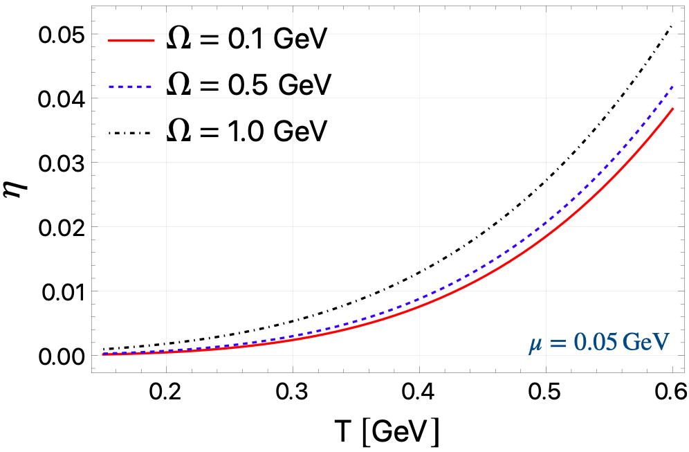
Figure 2: Behaviour of $\eta$ with $T$ for $\Omega$ = 0.1, 0.5, 1.0 GeV at $\mu$ = 0.05 GeV.

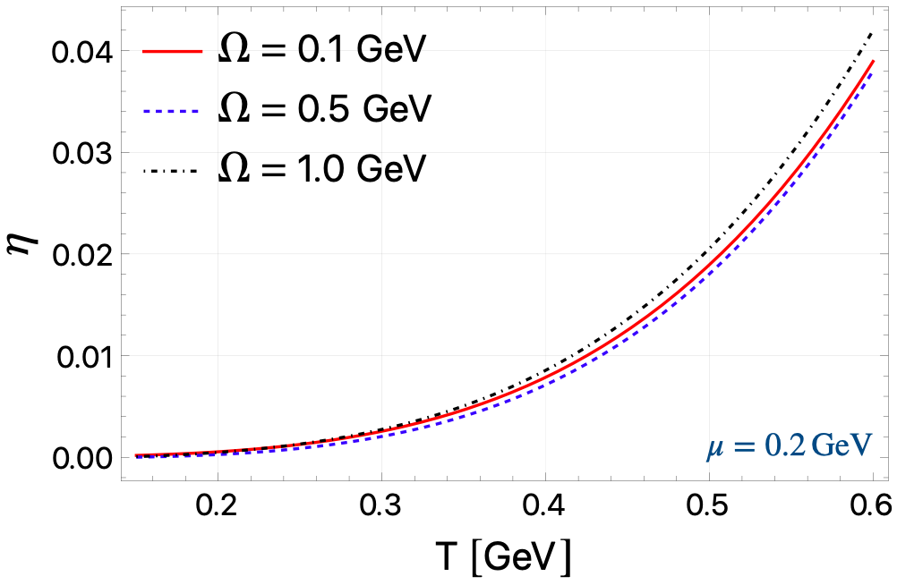
Figure 3: Same as fig. 2 but for $\mu$ = 0.2 GeV.

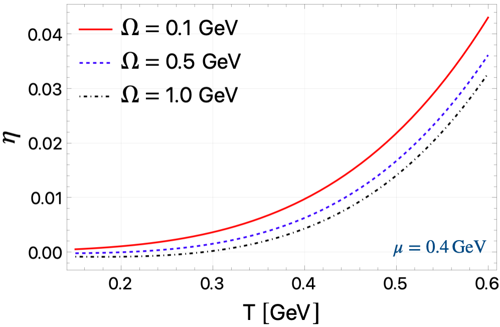
Figure 4: Same as fig. 2 but for $\mu$ = 0.4 GeV.

Our investigation predominantly characterizes QGP through its shear viscosity, although both shear and bulk viscosities are crucial. For a more comprehensive understanding of QGP’s phenomenological properties, it’s essential to focus on specific viscosities like shear viscosity to entropy density ratio ($\eta/s$) and bulk viscosity to entropy density ratio ($\zeta/s$). Our study provides a universal framework for examining the shear viscosity ($\eta$) in fermionic systems. It’s adaptable for exploring the dynamics of quarks and spin-$1/2$ baryons, offering insights into the broader scope of QGP properties.

In our study, as depicted in Figures 2 to 4, we analyze the variation of $\eta$ with $T$ across different $\mu$. In Figure 2, focusing on $\mu=0.05$ GeV, $\eta$ is examined over a temperature range from 0.15 to 0.6 GeV for various angular velocities ($\Omega$ values of 0.1, 0.5, and 1 GeV). This analysis reveals that $\eta$ typically increases with temperature, a characteristic behavior of relativistic fluids. Notably, $\eta$ also shows an increase with $\Omega$, particularly in the lower temperature range. This trend aligns with expectations, but may not hold for smaller $\Omega$ values (below 0.1 GeV), considering the limitations of our employed propagator, which is more accurate for larger $\Omega$ values. The increasing nature of $\eta$ with $\Omega$ may be deduced mathematically from Eq. (34), where the expression shows that there is a $\mathcal{O}(\Omega^{4})$ dependence of $\eta$ on $\Omega$. Additionally, in a rotating fluid, the shear flow induced by velocity gradients is further amplified by the rotation, as the velocity $v=\Omega r$ and its gradient $\vec{\nabla}v\sim\mathcal{O}(\Omega)$ introduce an extra $\Omega$-dependent velocity gradient into the system, contributing to an increase in shear viscosity.

In Figures 3 and 4, we observe a similar increasing trend of shear viscosity ($\eta$) with temperature ($T$) but with notable differences. In Figure 3, plotted for $\mu=0.2$ GeV, the curve for $\Omega=0.1$ GeV interestingly positions itself between the curves for $\Omega=0.5$ GeV and $1.0$ GeV. The trend completely reverses in Fig. 4 as compared to Fig. 2.

These observations reveal a complex interplay between the $\mu$ and $\Omega$. Both factors influence the distribution functions, but $\Omega$ additionally appears in the numerator of the $\eta$ expression, subtly altering its impact. As $\mu$ increases, its influence seems to suppress the effects of $\Omega$. This behavior is constrained by physical limits, particularly causality concerns, which restrict the allowable values of $\Omega$. Excessively large $\Omega$ values could lead to particles escaping the system’s confines, violating physical constraints. These results suggest that while temperature and angular velocity generally enhance each other, leading to potentially higher angular velocities at higher temperatures in collider experiments, the chemical potential exerts a contrasting effect. As $\mu$ increases, the suppression of $\Omega$’s influence becomes more pronounced, indicating a delicate balance between these parameters in the dynamics of rotating fermionic systems like the QGP.

V Summary

In a medium undergoing finite rotation, transport coefficients are influenced and exhibit a dependency on the medium’s angular velocity. Utilizing the Kubo formalism, this study quantifies the shear viscosity in a generalized fermionic system subjected to high angular velocity. The impact of angular velocity is integrated into the calculations through the momentum space propagator of the fermion, obtained via the Fock-Schwinger approach. This influence manifests in the distribution function via Matsubara frequency summation and also appears in the numerator of the shear viscosity expression through trace evaluations. Our findings indicate that shear viscosity rises with increasing temperature and angular velocity, while it diminishes with higher chemical potential. Notably, the chemical potential and its functional equivalent, the angular velocity, exert contrasting effects on the dissipation via shear viscosity in fermionic systems. Research to generalize these findings for arbitrary strengths of angular velocity is ongoing, and those outcomes will be reported in future work.

References

- [1] S. A. Bass, M. Gyulassy, H. Stoecker, and W. Greiner, “Signatures of quark gluon plasma formation in high-energy heavy ion collisions: A Critical review,” J. Phys. G 25 (1999) R1–R57, arXiv:hep-ph/9810281.
- [2] D. Kharzeev and M. Nardi, “Hadron production in nuclear collisions at RHIC and high density QCD,” Phys. Lett. B 507 (2001) 121–128, arXiv:nucl-th/0012025.
- [3] U. W. Heinz and P. F. Kolb, “Early thermalization at RHIC,” Nucl. Phys. A 702 (2002) 269–280, arXiv:hep-ph/0111075.
- [4] E. V. Shuryak, “What RHIC experiments and theory tell us about properties of quark-gluon plasma?,” Nucl. Phys. A 750 (2005) 64–83, arXiv:hep-ph/0405066.
- [5] M. Gyulassy and L. McLerran, “New forms of QCD matter discovered at RHIC,” Nucl. Phys. A 750 (2005) 30–63, arXiv:nucl-th/0405013.
- [6] W. Florkowski, Phenomenology of ultra-relativistic heavy-ion collisions. World Scientific, Singapore, 2010. https://cds.cern.ch/record/1321594.
- [7] B. V. Jacak and B. Muller, “The exploration of hot nuclear matter,” Science 337 (2012) 310–314.
- [8] D. Kharzeev, K. Landsteiner, A. Schmitt, and H.-U. Yee, eds., Strongly Interacting Matter in Magnetic Fields, vol. 871. Springer, 2013.
- [9] K. Hattori and X.-G. Huang, “Novel quantum phenomena induced by strong magnetic fields in heavy-ion collisions,” Nucl. Sci. Tech. 28 no. 2, (2017) 26, arXiv:1609.00747 [nucl-th].
- [10] Y. Hidaka, S. Pu, Q. Wang, and D.-L. Yang, “Foundations and applications of quantum kinetic theory,” Prog. Part. Nucl. Phys. 127 (2022) 103989, arXiv:2201.07644 [hep-ph].
- [11] F. Becattini, J. Liao, and M. Lisa, “Strongly Interacting Matter Under Rotation: An Introduction,” Lect. Notes Phys. 987 (2021) 1–14, arXiv:2102.00933 [nucl-th].
- [12] P. Romatschke and U. Romatschke, “Viscosity Information from Relativistic Nuclear Collisions: How Perfect is the Fluid Observed at RHIC?,” Phys. Rev. Lett. 99 (2007) 172301, arXiv:0706.1522 [nucl-th].
- [13] U. Heinz and R. Snellings, “Collective flow and viscosity in relativistic heavy-ion collisions,” Ann. Rev. Nucl. Part. Sci. 63 (2013) 123–151, arXiv:1301.2826 [nucl-th].
- [14] D. T. Son and A. O. Starinets, “Hydrodynamics of r-charged black holes,” JHEP 03 (2006) 052, arXiv:hep-th/0601157.
- [15] T. Schäfer and D. Teaney, “Nearly Perfect Fluidity: From Cold Atomic Gases to Hot Quark Gluon Plasmas,” Rept. Prog. Phys. 72 (2009) 126001, arXiv:0904.3107 [hep-ph].
- [16] B. Schenke, “The smallest fluid on Earth,” Rept. Prog. Phys. 84 no. 8, (2021) 082301, arXiv:2102.11189 [nucl-th].
- [17] W. Florkowski, M. P. Heller, and M. Spalinski, “New theories of relativistic hydrodynamics in the LHC era,” Rept. Prog. Phys. 81 no. 4, (2018) 046001, arXiv:1707.02282 [hep-ph].
- [18] STAR Collaboration, L. Adamczyk et al., “Global hyperon polarization in nuclear collisions: evidence for the most vortical fluid,” Nature 548 (2017) 62–65, arXiv:1701.06657 [nucl-ex].
- [19] STAR Collaboration, J. Adam et al., “Global polarization of hyperons in Au+Au collisions at = 200 GeV,” Phys. Rev. C98 (2018) 014910, arXiv:1805.04400 [nucl-ex].
- [20] STAR Collaboration, J. Adam et al., “Polarization of () hyperons along the beam direction in Au+Au collisions at = 200 GeV,” Phys. Rev. Lett. 123 no. 13, (2019) 132301, arXiv:1905.11917 [nucl-ex].
- [21] ALICE Collaboration, S. Acharya et al., “Evidence of Spin-Orbital Angular Momentum Interactions in Relativistic Heavy-Ion Collisions,” Phys. Rev. Lett. 125 no. 1, (2020) 012301, arXiv:1910.14408 [nucl-ex].
- [22] ALICE Collaboration, S. Acharya et al., “Global polarization of hyperons in Pb-Pb collisions at = 2.76 and 5.02 TeV,” Phys. Rev. C 101 no. 4, (2020) 044611, arXiv:1909.01281 [nucl-ex].
- [23] ALICE Collaboration, S. Acharya et al., “Polarization of and Hyperons along the Beam Direction in Pb-Pb Collisions at =5.02 TeV,” Phys. Rev. Lett. 128 no. 17, (2022) 172005, arXiv:2107.11183 [nucl-ex].
- [24] D. T. Son and P. Surowka, “Hydrodynamics with Triangle Anomalies,” Phys. Rev. Lett. 103 (2009) 191601, arXiv:0906.5044 [hep-th].
- [25] D. E. Kharzeev and D. T. Son, “Testing the chiral magnetic and chiral vortical effects in heavy ion collisions,” Phys. Rev. Lett. 106 (2011) 062301, arXiv:1010.0038 [hep-ph].
- [26] W. Florkowski, B. Friman, A. Jaiswal, and E. Speranza, “Relativistic fluid dynamics with spin,” Phys. Rev. C 97 no. 4, (2018) 041901, arXiv:1705.00587 [nucl-th].
- [27] W. Florkowski, B. Friman, A. Jaiswal, R. Ryblewski, and E. Speranza, “Spin-dependent distribution functions for relativistic hydrodynamics of spin-1/2 particles,” Phys. Rev. D97 no. 11, (2018) 116017, arXiv:1712.07676 [nucl-th].
- [28] W. Florkowski, A. Kumar, and R. Ryblewski, “Thermodynamic versus kinetic approach to polarization-vorticity coupling,” Phys. Rev. C98 no. 4, (2018) 044906, arXiv:1806.02616 [hep-ph].
- [29] W. Florkowski, A. Kumar, and R. Ryblewski, “Relativistic hydrodynamics for spin-polarized fluids,” Prog. Part. Nucl. Phys. 108 (2019) 103709, arXiv:1811.04409 [nucl-th].
- [30] W. Florkowski, A. Kumar, R. Ryblewski, and R. Singh, “Spin polarization evolution in a boost invariant hydrodynamical background,” Phys. Rev. C 99 no. 4, (2019) 044910, arXiv:1901.09655 [hep-ph].
- [31] R. Singh, M. Shokri, and R. Ryblewski, “Spin polarization dynamics in the Bjorken-expanding resistive MHD background,” Phys. Rev. D 103 no. 9, (2021) 094034, arXiv:2103.02592 [hep-ph].
- [32] W. Florkowski, R. Ryblewski, R. Singh, and G. Sophys, “Spin polarization dynamics in the non-boost-invariant background,” Phys. Rev. D 105 no. 5, (2022) 054007, arXiv:2112.01856 [hep-ph].
- [33] S. Bhadury, W. Florkowski, A. Jaiswal, A. Kumar, and R. Ryblewski, “Relativistic dissipative spin dynamics in the relaxation time approximation,” Phys. Lett. B 814 (2021) 136096, arXiv:2002.03937 [hep-ph].
- [34] S. Bhadury, W. Florkowski, A. Jaiswal, A. Kumar, and R. Ryblewski, “Dissipative Spin Dynamics in Relativistic Matter,” Phys. Rev. D 103 no. 1, (2021) 014030, arXiv:2008.10976 [nucl-th].
- [35] K. Hattori, M. Hongo, X.-G. Huang, M. Matsuo, and H. Taya, “Fate of spin polarization in a relativistic fluid: An entropy-current analysis,” Phys. Lett. B 795 (2019) 100–106, arXiv:1901.06615 [hep-th].
- [36] K. Fukushima and S. Pu, “Spin hydrodynamics and symmetric energy-momentum tensors – A current induced by the spin vorticity –,” Phys. Lett. B 817 (2021) 136346, arXiv:2010.01608 [hep-th].
- [37] S. Li, M. A. Stephanov, and H.-U. Yee, “Nondissipative Second-Order Transport, Spin, and Pseudogauge Transformations in Hydrodynamics,” Phys. Rev. Lett. 127 no. 8, (2021) 082302, arXiv:2011.12318 [hep-th].
- [38] D. Montenegro and G. Torrieri, “Linear response theory and effective action of relativistic hydrodynamics with spin,” Phys. Rev. D 102 no. 3, (2020) 036007, arXiv:2004.10195 [hep-th].
- [39] N. Weickgenannt, E. Speranza, X.-l. Sheng, Q. Wang, and D. H. Rischke, “Generating Spin Polarization from Vorticity through Nonlocal Collisions,” Phys. Rev. Lett. 127 no. 5, (2021) 052301, arXiv:2005.01506 [hep-ph].
- [40] M. Garbiso and M. Kaminski, “Hydrodynamics of simply spinning black holes & hydrodynamics for spinning quantum fluids,” JHEP 12 (2020) 112, arXiv:2007.04345 [hep-th].
- [41] A. D. Gallegos, U. Gürsoy, and A. Yarom, “Hydrodynamics of spin currents,” SciPost Phys. 11 (2021) 041, arXiv:2101.04759 [hep-th].
- [42] X.-L. Sheng, N. Weickgenannt, E. Speranza, D. H. Rischke, and Q. Wang, “From Kadanoff-Baym to Boltzmann equations for massive spin-1/2 fermions,” Phys. Rev. D 104 no. 1, (2021) 016029, arXiv:2103.10636 [nucl-th].
- [43] E. Speranza and N. Weickgenannt, “Spin tensor and pseudo-gauges: from nuclear collisions to gravitational physics,” Eur. Phys. J. A 57 no. 5, (2021) 155, arXiv:2007.00138 [nucl-th].
- [44] F. Becattini, I. Karpenko, M. Lisa, I. Upsal, and S. Voloshin, “Global hyperon polarization at local thermodynamic equilibrium with vorticity, magnetic field and feed-down,” Phys. Rev. C95 no. 5, (2017) 054902, arXiv:1610.02506 [nucl-th].
- [45] I. Karpenko and F. Becattini, “Study of polarization in relativistic nuclear collisions at –200 GeV,” Eur. Phys. J. C77 no. 4, (2017) 213, arXiv:1610.04717 [nucl-th].
- [46] L.-G. Pang, H. Petersen, Q. Wang, and X.-N. Wang, “Vortical Fluid and Spin Correlations in High-Energy Heavy-Ion Collisions,” Phys. Rev. Lett. 117 no. 19, (2016) 192301, arXiv:1605.04024 [hep-ph].
- [47] Y. Xie, D. Wang, and L. P. Csernai, “Global polarization in high energy collisions,” Phys. Rev. C 95 no. 3, (2017) 031901, arXiv:1703.03770 [nucl-th].
- [48] F. Becattini and I. Karpenko, “Collective Longitudinal Polarization in Relativistic Heavy-Ion Collisions at Very High Energy,” Phys. Rev. Lett. 120 no. 1, (2018) 012302, arXiv:1707.07984 [nucl-th].
- [49] B. Fu, K. Xu, X.-G. Huang, and H. Song, “Hydrodynamic study of hyperon spin polarization in relativistic heavy ion collisions,” Phys. Rev. C 103 no. 2, (2021) 024903, arXiv:2011.03740 [nucl-th].
- [50] W. Florkowski, A. Kumar, A. Mazeliauskas, and R. Ryblewski, “Effect of thermal shear on longitudinal spin polarization in a thermal model,” Phys. Rev. C 105 no. 6, (2022) 064901, arXiv:2112.02799 [hep-ph].
- [51] D. Montenegro and G. Torrieri, “Causality and dissipation in relativistic polarizable fluids,” Phys. Rev. D 100 no. 5, (2019) 056011, arXiv:1807.02796 [hep-th].
- [52] W. M. Serenone, J. a. G. P. Barbon, D. D. Chinellato, M. A. Lisa, C. Shen, J. Takahashi, and G. Torrieri, “ polarization from thermalized jet energy,” Phys. Lett. B 820 (2021) 136500, arXiv:2102.11919 [hep-ph].
- [53] G. Torrieri and D. Montenegro, “Linear response hydrodynamics of a relativistic dissipative fluid with spin,” Phys. Rev. D 107 no. 7, (2023) 076010, arXiv:2207.00537 [hep-th].
- [54] A. Daher, A. Das, W. Florkowski, and R. Ryblewski, “Canonical and phenomenological formulations of spin hydrodynamics,” Phys. Rev. C 108 no. 2, (2023) 024902, arXiv:2202.12609 [nucl-th].
- [55] Z. Cao, K. Hattori, M. Hongo, X.-G. Huang, and H. Taya, “Gyrohydrodynamics: Relativistic spinful fluid with strong vorticity,” PTEP 2022 no. 7, (2022) 071D01, arXiv:2205.08051 [hep-th].
- [56] J. Hu, “Kubo formulae for first-order spin hydrodynamics,” Phys. Rev. D 103 no. 11, (2021) 116015, arXiv:2101.08440 [hep-ph].
- [57] Y. Hidaka and D.-L. Yang, “Nonequilibrium chiral magnetic/vortical effects in viscous fluids,” Phys. Rev. D 98 no. 1, (2018) 016012, arXiv:1801.08253 [hep-th].
- [58] D.-L. Yang, K. Hattori, and Y. Hidaka, “Effective quantum kinetic theory for spin transport of fermions with collsional effects,” JHEP 20 (2020) 070, arXiv:2002.02612 [hep-ph].
- [59] Z. Wang, X. Guo, and P. Zhuang, “Equilibrium Spin Distribution From Detailed Balance,” Eur. Phys. J. C 81 no. 9, (2021) 799, arXiv:2009.10930 [hep-th].
- [60] N. Weickgenannt, E. Speranza, X.-l. Sheng, Q. Wang, and D. H. Rischke, “Derivation of the nonlocal collision term in the relativistic Boltzmann equation for massive spin-1/2 particles from quantum field theory,” Phys. Rev. D 104 no. 1, (2021) 016022, arXiv:2103.04896 [nucl-th].
- [61] J. Hu, “Relativistic first-order spin hydrodynamics via the Chapman-Enskog expansion,” Phys. Rev. D 105 no. 7, (2022) 076009, arXiv:2111.03571 [hep-ph].
- [62] A. Das, W. Florkowski, A. Kumar, R. Ryblewski, and R. Singh, “Semi-classical Kinetic Theory for Massive Spin-half Fermions with Leading-order Spin Effects,” Acta Phys. Polon. B 54 no. 8, (2023) 8–A4, arXiv:2203.15562 [hep-th].
- [63] N. Weickgenannt, D. Wagner, E. Speranza, and D. H. Rischke, “Relativistic second-order dissipative spin hydrodynamics from the method of moments,” Phys. Rev. D 106 no. 9, (2022) 096014, arXiv:2203.04766 [nucl-th].
- [64] M. A. Stephanov and Y. Yin, “Chiral Kinetic Theory,” Phys. Rev. Lett. 109 (2012) 162001, arXiv:1207.0747 [hep-th].
- [65] J.-Y. Chen, D. T. Son, M. A. Stephanov, H.-U. Yee, and Y. Yin, “Lorentz Invariance in Chiral Kinetic Theory,” Phys. Rev. Lett. 113 no. 18, (2014) 182302, arXiv:1404.5963 [hep-th].
- [66] E. V. Gorbar, D. O. Rybalka, and I. A. Shovkovy, “Second-order dissipative hydrodynamics for plasma with chiral asymmetry and vorticity,” Phys. Rev. D95 no. 9, (2017) 096010, arXiv:1702.07791 [hep-th].
- [67] S. Shi, C. Gale, and S. Jeon, “From chiral kinetic theory to relativistic viscous spin hydrodynamics,” Phys. Rev. C 103 no. 4, (2021) 044906, arXiv:2008.08618 [nucl-th].
- [68] M. P. Heller, A. Serantes, M. Spaliński, V. Svensson, and B. Withers, “Convergence of hydrodynamic modes: insights from kinetic theory and holography,” SciPost Phys. 10 no. 6, (2021) 123, arXiv:2012.15393 [hep-th].
- [69] A. D. Gallegos and U. Gürsoy, “Holographic spin liquids and Lovelock Chern-Simons gravity,” JHEP 11 (2020) 151, arXiv:2004.05148 [hep-th].
- [70] M. Hongo, X.-G. Huang, M. Kaminski, M. Stephanov, and H.-U. Yee, “Relativistic spin hydrodynamics with torsion and linear response theory for spin relaxation,” JHEP 11 (2021) 150, arXiv:2107.14231 [hep-th].
- [71] A. D. Gallegos, U. Gursoy, and A. Yarom, “Hydrodynamics, spin currents and torsion,” JHEP 05 (2023) 139, arXiv:2203.05044 [hep-th].
- [72] R. Singh, “Collective dynamics of polarized spin-half fermions in relativistic heavy-ion collisions,” Int. J. Mod. Phys. A 38 no. 20, (2023) 2330011, arXiv:2212.06569 [hep-ph].
- [73] R. Singh, M. Shokri, and S. M. A. T. Mehr, “Relativistic hydrodynamics with spin in the presence of electromagnetic fields,” Nucl. Phys. A 1035 (2023) 122656, arXiv:2202.11504 [hep-ph].
- [74] R. Singh, “Theoretical Aspects of Relativistic Perfect-fluid Spin Hydrodynamic Framework,” Acta Phys. Polon. Supp. 15 no. 3, (2022) 35.
- [75] D. Kharzeev and A. Zhitnitsky, “Charge separation induced by P-odd bubbles in QCD matter,” Nucl. Phys. A 797 (2007) 67–79, arXiv:0706.1026 [hep-ph].
- [76] Y. Burnier, D. E. Kharzeev, J. Liao, and H.-U. Yee, “Chiral magnetic wave at finite baryon density and the electric quadrupole moment of quark-gluon plasma in heavy ion collisions,” Phys. Rev. Lett. 107 (2011) 052303, arXiv:1103.1307 [hep-ph].
- [77] D. E. Kharzeev, J. Liao, S. A. Voloshin, and G. Wang, “Chiral magnetic and vortical effects in high-energy nuclear collisions – status report,” Prog. Part. Nucl. Phys. 88 (2016) 1–28, arXiv:1511.04050 [hep-ph].
- [78] Y. Jiang, X.-G. Huang, and J. Liao, “Chiral vortical wave and induced flavor charge transport in a rotating quark-gluon plasma,” Phys. Rev. D 92 no. 7, (2015) 071501, arXiv:1504.03201 [hep-ph].
- [79] Y. J. Minghua Wei and and M. Huang, “Mass splitting of vector mesons and spontaneous spin polarization under rotation *,” Chin. Phys. C 46 no. 2, (2022) 024102, arXiv:2011.10987 [hep-ph].
- [80] H. M. Ghalati and N. Sadooghi, “The magnetic dual chiral density wave phase in a rotating quark matter,” arXiv:2306.04472 [nucl-th].
- [81] V. E. Ambrus and E. Winstanley, “Vortical Effects for Free Fermions on Anti-De Sitter Space-Time,” Symmetry 13 (2021) 2019, arXiv:2107.06928 [hep-th].
- [82] M. N. Chernodub, “Inhomogeneous confining-deconfining phases in rotating plasmas,” Phys. Rev. D 103 no. 5, (2021) 054027, arXiv:2012.04924 [hep-ph].
- [83] N. Sadooghi, S. M. A. Tabatabaee Mehr, and F. Taghinavaz, “Inverse magnetorotational catalysis and the phase diagram of a rotating hot and magnetized quark matter,” Phys. Rev. D 104 no. 11, (2021) 116022, arXiv:2108.12760 [hep-ph].
- [84] V. V. Braguta, M. N. Chernodub, A. A. Roenko, and D. A. Sychev, “Negative moment of inertia and rotational instability of gluon plasma,” arXiv:2303.03147 [hep-lat].
- [85] A. Harutyunyan and A. Sedrakian, “Bulk Viscosity of Hot Quark Plasma from Non-Equilibrium Statistical Operator,” Particles 1 no. 1, (2018) 212–229, arXiv:1808.06403 [nucl-th].
- [86] A. Harutyunyan, A. Sedrakian, and D. H. Rischke, “Relativistic second-order dissipative hydrodynamics from Zubarev’s non-equilibrium statistical operator,” Annals Phys. 438 (2022) 168755, arXiv:2110.04595 [nucl-th].
- [87] A. Czajka, K. Dasgupta, C. Gale, S. Jeon, A. Misra, M. Richard, and K. Sil, “Bulk Viscosity at Extreme Limits: From Kinetic Theory to Strings,” JHEP 07 (2019) 145, arXiv:1807.04713 [hep-th].
- [88] F. Becattini, M. Buzzegoli, and E. Grossi, “Reworking the Zubarev’s approach to non-equilibrium quantum statistical mechanics,” Particles 2 no. 2, (2019) 197–207, arXiv:1902.01089 [cond-mat.stat-mech].
- [89] F. W. Hehl, P. Von Der Heyde, G. D. Kerlick, and J. M. Nester, “General Relativity with Spin and Torsion: Foundations and Prospects,” Rev. Mod. Phys. 48 (1976) 393–416.
- [90] A. Kuznetsov and N. Mikheev, “Electroweak processes in external electromagnetic fields,” Springer Tracts Mod. Phys. 197 (2004) 1–120.
- [91] A. Kuznetsov and N. Mikheev, eds., Electroweak Processes in External Active Media, vol. 252 of Springer Tracts in Modern Physics. 2013.
- [92] T.-K. Chyi, C.-W. Hwang, W. F. Kao, G.-L. Lin, K.-W. Ng, and J.-J. Tseng, “The weak field expansion for processes in a homogeneous background magnetic field,” Phys. Rev. D 62 (2000) 105014, arXiv:hep-th/9912134.
- [93] S. N. Iablokov and A. V. Kuznetsov, “Charged massive vector boson propagator in a constant magnetic field in arbitrary -gauge obtained using the modified Fock-Schwinger method,” Phys. Rev. D 102 no. 9, (2020) 096015, arXiv:2008.07890 [hep-th].
- [94] A. Ayala, L. A. Hernández, K. Raya, and R. Zamora, “Fermion propagator in a rotating environment,” Phys. Rev. D 103 no. 7, (2021) 076021, arXiv:2102.03476 [hep-ph]. [Erratum: Phys.Rev.D 104, 039901 (2021)].
- [95] R.-H. Fang, “Thermodynamics for a Rotating Chiral Fermion System in the Uniform Magnetic Field,” Symmetry 14 no. 6, (2022) 1106, arXiv:2112.03468 [hep-th].
- [96] R. Singh, G. Sophys, and R. Ryblewski, “Spin polarization dynamics in the Gubser-expanding background,” Phys. Rev. D 103 no. 7, (2021) 074024, arXiv:2011.14907 [hep-ph].
- [97] M. Wei, C. A. Islam, and M. Huang, “Production rate and ellipticity of lepton pairs from a rotating hot and dense QCD medium,” Phys. Rev. D 105 no. 5, (2022) 054014, arXiv:2111.05192 [hep-ph].
- [98] M. Laine and A. Vuorinen, Basics of Thermal Field Theory, vol. 925. Springer, 2016. arXiv:1701.01554 [hep-ph].
- [99] S. Mallik and S. Sarkar, Hadrons at Finite Temperature. Cambridge University Press, Cambridge, 2016.
- [100] R. Lang, N. Kaiser, and W. Weise, “Shear Viscosity of a Hot Pion Gas,” Eur. Phys. J. A 48 (2012) 109, arXiv:1205.6648 [hep-ph].