Solving Systems of Linear Equations: HHL from a Tensor Networks Perspective

Abstract

We present an algorithm for solving systems of linear equations based on the HHL algorithm with a novel qudits methodology, a generalization of the qubits with more states, to reduce the number of gates to be applied and the amount of resources. Based on this idea, we will perform a quantum-inspired version on tensor networks, taking advantage of their ability to perform non-unitary operations such as projection. Finally, we will use this algorithm to obtain a solution for the harmonic oscillator with an external force, the forced damped oscillator and the 2D static heat equation differential equations.

1 Introduction

Solving linear equation systems $A\vec{x}=\vec{b}$ is a fundamental problem in many areas of science and engineering. Classical methods for solving these equations, such as Gaussian elimination and LU decomposition [1], have been widely used and optimized for decades. However, as the size of the system grows, classical methods become computationally expensive and inefficient. One of the most efficient classical methods is the conjugate gradient method (CG)[2], which is of order $O(Ns\kappa\log\left(\frac{1}{\epsilon}\right))$ for a matrix $N\times N$ with a maximum of $s$ no null elements per row, $\kappa\equiv\frac{\lambda_{max}}{\lambda_{min}}$, being $\lambda$ the eigenvalues of the matrix $A$, and $\epsilon$ the error.

Quantum computers offer the potential to solve some of the most challenging problems more efficiently than classical computers. In particular, the HHL algorithm proposed by Harrow, Hassidim, and Lloyd in 2008 [3] is a method for solving linear equations that runs in polynomial time, where the polynomial depends logarithmically on the size of the system. However, it is intended for the calculation of expected values in $O\left(\log(N)s^{2}\kappa^{2}/\epsilon\right)$, since it loses its advantage in the case of wanting to obtain the solution directly.

Recently, there has been growing interest in using qudits and tensor networks [4] to implement different quantum algorithms. Qudits are generalized qubits, with more than 2 basis states, while tensor networks provide an efficient way to represent and manipulate high-dimensional quantum states with low entanglement and calculate quickly with them in classical computers [5] [6].

In this paper, we propose a novel approach for solving linear equations using qudits and tensor networks. We demonstrate how this approach can be used to efficiently solve linear systems with a large number of variables, and we compare the performance of our approach with existing quantum and classical methods. Our results show that our approach can achieve a promising performance in computational efficiency for solving linear equations and simulate the HHL process without quantum noise.

2 HHL Algorithm

Fistly, we will briefly introduce the standard HHL algorithm in qubits in order to better understand the algorithm we will formalize.

This algorithm solves the system of linear equations

$$A\vec{x}=\vec{b},$$ (1)

where $A$ is an invertible matrix $N\times N$, $\vec{x}$ is the vector we want to obtain and $\vec{b}$ is another vector, both with dimension $N$.

For this algorithm we will need $n$ qubits so that $2^{n}\geq N$ to encode the vector $\vec{b}$, $n_{c}$ clock qubits to encode the eigenvalues of $A$ and one auxiliary qubit for the inversion. The whole process can be summarized in Fig. 1.

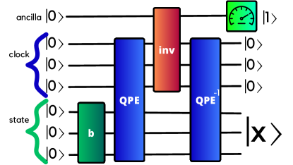
Figure 1: Quantum HHL in qubits.

We encode the state $\vec{b}$ in the amplitudes of the $n$ state qubits

$$|b\rangle=\sum_{i=0}^{2^{n}-1}b_{i}|i\rangle=\sum_{i=0}^{2^{n}-1}\beta_{i}|u_{i}\rangle$$ (2)

where $b_{i}$ are the normalized components of vector $\vec{b}$, $|i\rangle$ are the binary computational bases and $|u_{i}\rangle$ the eigenvector associated to the eigenvalue $\lambda_{i}$ of $A$. We use a operator $b$ to initialize it.

It is important to note that the difference between $N$ and $2^{n}$ will be covered by 0 in the vector and a matrix proportional to the identity in A, wasting resources. Moreover, we need a method to generate this state $|b\rangle$.

The second thing we will do is calculate the operator

$$U=e^{iA^{\prime}t},$$ (3)

being $A^{\prime}=A$ the matrix if it is hermitian, and

$$A^{\prime}=\left(\begin{matrix}0&A\\ A^{\dagger}&0\end{matrix}\right)$$ (4)

if it is not. In this case the problem is

$$A^{\prime}\left(\begin{matrix}0\\ \vec{x}\end{matrix}\right)=\left(\begin{matrix}\vec{b}\\ 0\end{matrix}\right)$$ (5)

We will assume $U$ can be calculated and implemented efficiently.

With this operator $U$ implemented, we perform a Quantum Phase Estimation (QPE) to encode the eigenvalues of $A^{\prime}$ in the clock qubits. Now we apply an inversion operator, which rotates the probability of the auxiliary qubit so that it is divided by the value of the eigenvalue encoded by the QPE.

The next step is making a post-selection, keeping only the state if the auxiliary qubit outputs a 1, followed by an inverse QPE to clean the eigenvalue qubits.

At the end, we have the $\vec{x}$-state normalized in the amplitudes,

$$|x\rangle=\frac{1}{\mathcal{N}}\sum_{i=0}^{2^{n}-1}\frac{\beta_{i}}{\lambda_{i}}|u_{i}\rangle=\frac{1}{\mathcal{N}}\sum_{i=0}^{2^{n}-1}x_{i}|i\rangle,$$ (6)

with a normalization constant $\mathcal{N}$ and omitting the ancilla and clock qubits.

To obtain the full state, we have to first obtain the amplitude distribution, so the HHL is usually applied to obtain the expected value of some quantity with respect to the solution.

The main problems of the algorithm are:

1. Large amount and waste of resources due to the difference between the size of the problem and the qubits to encode it.

2. Circuit depth and errors introduced by the QPE.

3. We do not get $\vec{x}$ directly, and if we extract it, we get it with a sign ambiguity for each of its elements.

4. Preparing state $\vec{b}$ may not be trivial, just like making the inversion operator or making the U-operator.

3 Qudit quantum algorithm

To try to overcome the two first problems of the HHL, we will formalize a qudit version of the algorithm. To do so, we will assume that there are quantum computers which implement the basic qudit gates at our disposal are those of paper [7].

The first thing we will do is to encode the state $\vec{b}$ in a single qudit. In case the qudit does not have enough states available, we will encode it in a number of qudits that allows us to encode it in a way analogous to the case of qubits. We will assume in the following that we only need one qudit with $N$ base states in order to clearly explain the algorithm.

Now we will need a way to simulate the $U=e^{iA^{\prime}t}$ operator, which would depend on the particular case we are dealing with.

With this, we will make the following circuit in Fig. 2.

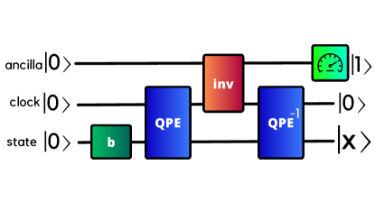
Figure 2: Quantum HHL in qudits.

With a single qudit of dimension $m=2^{n_{c}}$ we can do the QPE as in [7] and encode the eigenvalues in its basis states amplitudes. However, we could use more qudits. If we use 2 qudits to encode $m$ values, each one will have to have dimension $\sqrt{m}$.

The inverter will be exactly the same as in the case of qubits, but instead of having a control-non-control series, we will have a control $i$ that will apply the rotation gate on the ancilla if we have the value $i$ in the qudit.

We do the post-selection and if we get $|1\rangle$, we perform the inverse QPE to clear the qudit of the eigenvalues.

With this we can see that we reduce the number of SWAP gates needed and the QPE is performed with a lower number of gates. Also, we waste less resources, as we can better adjust the dimensionality of the quantum system with respect to the equation to be solved. Moreover, in the best case scenario we only need two qudits and one qubit.

Still, we could do more to solve the other problems, so let’s try to tackle them with the quantum-inspired technique of tensor networks, avoiding the gate errors from the quantum devices and extract directly the $\vec{x}$.

4 Tensor Networks Algorithm

We are going to convert the qudit circuit into a tensor network, so that it returns the vector $\vec{x}$ directly. This method will be a tensor network HHL (TN HHL). Since in tensor networks we do not need the normalization, we will not normalize the state $|b\rangle$. As it is not normalized, the result state will not be normalized either, so we will not have to rescale it. Moreover, the state can be prepared exactly in a single operation, defining the node $\vec{b}$.

The QPE is performed contracting the uniform superposition state with the Quantum Fourier (QFT) Transform in the QPE, so we have a matrix $H_{m}$ with dimension $m\times m$ for $m$ eigenvalues with elements

$$\left(H_{m}\right)_{ab}=e^{2\pi i\frac{ab}{m}}$$ (7)

without normalization.

The inverter will be a non-unitary operator whose non-zero elements are

$$\left(\mbox{inv}_{m}\right)_{i,j}=\left\{\begin{array}[]{cl}\nicefrac{{1}}{{i}}&\mbox{ if }i=j\neq 0\mbox{ and if }i\leq\frac{m}{2}\\ \frac{1}{i-m}&\mbox{ if }i=j\mbox{ and if }i>\frac{m}{2}\end{array}\right.$$ (8)

In order to be able to encode negative eigenvalues due to the cyclic property of the imaginary exponential. If we want more positive or more negative eigenvalues, we must change the proportion of $i$-values which are translated as positive or negative eigenvalues.

The phase kickback operators can also be obtained exactly from $U$. This tensor $P$ would be

$$\left(P_{m}\right)_{i,j,k}=\left(U^{j}\right)_{i,k};\left(P^{-1}_{m}\right)_{i,j,k}=\left(\left(U^{-1}\right)^{j}\right)_{k,i}.$$ (9)

This tensors are contracted through their $j$ index with the $H_{m}$ and $H_{m}^{-1}$ tensors for doing the QPE.

With these tensors, we can get our result by contraction the tensor network in Fig. 3 a)

$$\sum_{a,b,c,d,e,f}b_{a}P_{abc}H^{-1}_{bd}\mbox{inv}_{de}H_{ef}P^{-1}_{cfi}=\frac{x_{i}m^{2}}{t}$$ (10)

with $b,c,d,e,f\in[0,m-1]$ and $a,c,i\in[0,N-1]$.

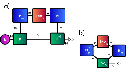
Figure 3: Tensor network equivalent to HHL. a) Original way. b) Eficient way.

The most efficient contraction for this tensor network has complexity $O\left(N^{2}m\right)+O\left(m^{3}\right)+O\left(Nm^{2}\right)$. However, the construction of the $P_{m}$ tensor requires $O(N^{3}m)$.

We could avoid this problem defining a tensor

$$(W_{m})_{ijk}=\left(\vec{b}U^{i-j}\right)_{k}$$ (11)

with a cost $O(N^{2}m)$. So, we have to contract the tensor network in Fig. 3 b)

$$\sum_{a,b,c,d}W_{abi}H^{-1}_{ac}\mbox{inv}_{cd}H_{db}=\frac{x_{i}m^{2}}{t}$$ (12)

which could be contracted in $O(m^{3})+O(Nm^{2})$. However, if we precalculate the contraction of $H_{m}$, $H^{-1}_{m}$ and $inv_{m}$ to use it every time, we could avoid the $O(m^{3})$.

Finally, the complexity of the method is $O(N^{2}m)+O(m^{2}N)+O(m^{3})$. The memory cost is $O(m^{2}N)+O(N^{2})$, being the first term associated with the $W_{m}$ tensor and the second term associated with the $U$ matrix.

We can also compute the inverse of $A^{\prime}$ just by erasing the $b$ node from Fig. 3 a) and doing the contraction, with a cost $O(m^{3})+O(N^{3}m)+O(N^{2}m^{2})$.

5 Comparison of advantages and disadvantages

We will compare the advantages and disadvantages of this algorithm in tensor networks against the conjugate gradient and quantum HHL in Table 1. We assume $m=O(\kappa)$. $m$ will also depend on the error bounds we want. Greater $m$ implies lower error bounds if we adjust properly the $t$. However, we have not being able to determine this scaling, but probably is a similar scaling as in the original HHL.

Notice we have not made us of the properties of the sparse matrices, as in the CG or the original HHL.

Algorithm	Inversion $A^{-1}$	Solution $\vec{x}=A^{-1}\vec{b}$	Expectation value $\vec{x^{T}}M\vec{x}$
CG	-	$O(Ns\kappa\log(1/\epsilon))$	$O(N\max(s\kappa\log(1/\epsilon),s^{\prime}))$
HHL	-	-	$O(\log(N)s^{2}\kappa^{2}/\epsilon)$
TN HHL	$O(N^{2}\kappa^{2})+O(N^{3}\kappa)+O(\kappa^{3})$	$O(N\kappa^{2})+O(N^{2}\kappa)+O(\kappa^{3})$	$O(\max(N^{2}\kappa,N\kappa^{2},\kappa^{3},Ns^{\prime}))$

Table 1: Computational times to invert a $N\times N$ matrix $A$, obtain the solution of $A\vec{x}=\vec{b}$ and compute an expected value $\langle x|M|x\rangle$. $s$ is the maximum number of non-zero elements per row of A and $s^{\prime}$ is the maximum number of non-zero elements per row of M.

5.1 TN HHL vs CG

We can see our algorithm is slower than the CG. However, the TN HHL can invert the matrix $A$. Moreover, both algorithms benefit from efficient matrix product algorithms. Also, if we have the eigenvalues, in the TN HHL we can change the $H_{m}$ and $W_{m}$ for wasting less resources using $m=n_{\lambda}$, being $n_{\lambda}$ the number of eigenvalues.

5.2 TN HHL vs HHL

The advantages of this TN HHL method over traditional quantum HHL are:

1. We do not waste resources, the QFT is a simple matrix and we do not need SWAP gates.

2. We can obtain the solution directly or some of its elements and we can get the right signs from our solutions. Also, we can obtain the inverse matrix.

3. We do not have to generate a complicated circuit for the initialization of the state and the time evolution of the phase kickback. Nor do we have the errors introduced by quantum gates.

4. We don’t use the post-selection.

However, when it comes to computing the expected value, it is indeed significantly less efficient in complexity.

6 Simulation

We will test the effectiveness of the method when performing numerical simulations. We will solve the forced harmonic oscillator, the forced damped oscillator and the 2D static heat equation with sources.

6.1 Forced harmonic oscillator

The differential equation we want to solve will be

$$\frac{d^{2}x}{dt^{2}}+\frac{k}{m}x=F(t)$$ (13)

$$x_{0}=x(t=0);\qquad x_{T}=x(t=T)$$

where $F(t)$ is the time-dependent external force. For the experiments we will use a force $F(t)=C\sin(\nu t)$.

We use the discretization with $n$ time-steps, being $\Omega=-2+\frac{k}{m}(\Delta t)^{2}$ and $F_{j}=(\Delta t)^{2}C\sin(\nu j\Delta t)$.

$$\left(\begin{matrix}\Omega&1&0&\cdots&0&0\\ 1&\Omega&1&\cdots&0&0\\ 0&1&\Omega&\cdots&0&0\\ \vdots&\vdots&\vdots&\ddots&\vdots&\vdots\\ 0&0&0&\cdots&1&\Omega\end{matrix}\right)\left(\begin{matrix}x_{1}\\ x_{2}\\ x_{3}\\ \vdots\\ x_{n}\end{matrix}\right)=\left(\begin{matrix}F_{1}-x_{0}\\ F_{2}\\ F_{3}\\ \vdots\\ F_{n}-x_{T}\end{matrix}\right)$$ (14)

The result of inverting this system gives us the result in Fig. 4. As hyperparameters of the method we use $m=2000$ and $t=6000$.

The root mean square error of our tensor network from the exact inversion was $1.8\times 10^{-5}$ and took $1.52$ s to run, compared with the $1.9$ ms of the Tensorflow method.

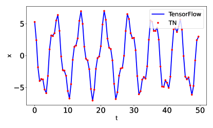
Figure 4: Solving the forced harmonic oscillator system with equation (14). In blue the inversion performed with Tensorflow and in red the inversion performed with the tensor network.

6.2 Forced damped oscillator

The differential equation we want to solve will be

$$\frac{d^{2}x}{dt^{2}}+\gamma\frac{dx}{dt}+\frac{k}{m}x=F(t)$$ (15)

$$x_{0}=x(t=0);\qquad x_{T}=x(t=T)$$

where $F(t)$ is the time-dependent external force and $\gamma$ is the damp coefficient. As in Ssec. 6.1, for the experiments we will use a force $F(t)=C\sin(\nu t)$.

We use the discretization with n time-steps

$$\left(\begin{matrix}\beta_{0}&\beta_{+}&0&\cdots&0&0\\ \beta_{-}&\beta_{0}&\beta_{+}&\cdots&0&0\\ 0&\beta_{-}&\beta_{0}&\cdots&0&0\\ \vdots&\vdots&\vdots&\ddots&\vdots&\vdots\\ 0&0&0&\cdots&\beta_{-}&\beta_{0}\end{matrix}\right)\left(\begin{matrix}x_{1}\\ x_{2}\\ x_{3}\\ \vdots\\ x_{n}\end{matrix}\right)=\left(\begin{matrix}F_{1}-\beta_{-}x_{0}\\ F_{2}\\ F_{3}\\ \vdots\\ F_{n}-\beta_{+}x_{T}\end{matrix}\right)$$ (16)

where $\beta_{-}=1-\gamma\frac{\Delta t}{2}$, $\beta_{+}=1+\gamma\frac{\Delta t}{2}$ and $\beta_{0}=-2+\frac{k}{m}(\Delta t)^{2}$. This matrix is not hermitian, so we apply (4) and solve (5).

The result of inverting this matrix gives us the result in Fig. 5. As hyperparameters of the method we use $m=2000$ and $t=1.1\times 10^{4}$.

The root mean square error of our tensor network from the exact inversion was $5.7\times 10^{-3}$ and took $10.6$ s to run, compared with the $2.6$ ms of the Tensorflow method.

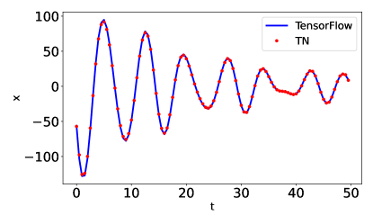
Figure 5: Solving the forced damped oscillator system with equation (16). In blue the inversion performed with Tensorflow and in red the inversion performed with the tensor network.

6.3 Static two dimensional heat equation with sources

The differential equation we want to solve will be

$$\kappa\left(\frac{d^{2}u}{dx^{2}}+\frac{d^{2}u}{dy^{2}}\right)=-S(x,y)$$ (17)

$$u_{x1}=u(0,y);\quad u_{x2}=u(L_{x},y)$$

$$u_{y}=u(x,0);\quad u_{y2}=u(x,L_{y})$$

where $S(x,y)$ is the position-dependent external source. For the experiments we will use a source $S(x,y)=10\sin(2\pi\frac{xy}{L_{x}L_{y}})$.

We will use the discretization

$$u_{j+1,k}+u_{j-1,k}+u_{j,k+1}+u_{j,k-1}-4u_{jk}=-(\Delta x)^{2}S_{jk}$$ (18)

We convert the 2-dimensional space into a line, create the matrix and obtain the following result in Figs. 6 and 7. As hyperparameters we use $m=2000$ and $t=100$.

The root mean square error of our tensor network from the exact inversion was $1\times 10^{-4}$ and took $37.9$ s to run, compared with the $11$ ms of the Tensorflow method.

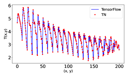
Figure 6: Solving the static two dimensional heat equation with sources with equation (18). In blue the inversion performed with Tensorflow and in red the inversion performed with the tensor network.

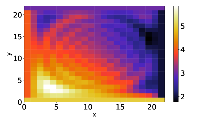
Figure 7: Solving the static two dimensional heat equation with sources with equation (18).

7 Conclusions

We have seen that our algorithm offers both a way to invert matrices, to solve linear equations and to perform numerical simulations based on it. We have also observed that its scaling is remarkably good with the size of the matrix to be inverted, while it can be realized on classical computers and accelerated with GPUs.

An advantage of this method is that it allows to observe the best possible theoretical result due to a quantum HHL, as it simulates what should happen without gate errors, post-selection problems or inaccuracies in state creation.

However, we have observed that the effective computational speed is remarkably low compared to methods already implemented in libraries such as Tensorflow or Numpy, mainly due to the creation time of the tensors.

The continuation of this line of research could be to find a way to improve the efficiency of the method in general by taking advantage of the characteristics of the tensors used, to improve the parallelisation of the calculations, to specialize it on tridiagonal matrices or extend it to complex eigenvalues.

References

-
[1]
A. Schwarzenberg-Czerny.
On matrix factorization and efficient least squares solution.
Astronomy and Astrophysics Supplement, v.110, p.405, (1995). -
[2]
Magnus R. Hestenes and Eduard Stiefel.
Methods of conjugate gradients for solving linear systems.
Journal of research of the National Bureau of Standards, pages 409-435, vol. 49, (1952). -
[3]
Aram W. Harrow, Avinatan Hassidim and Seth Lloyd.
Quantum algorithm for solving linear systems of equations.
arXiv:0811.3171 [quant-ph], (2008). -
[4]
Jacob Biamonte, Ville Bergholm.
Tensor Networks in a Nutshell.
arXiv:1708.00006 [quant-ph], (2017). -
[5]
Michael Lubasch, Pierre Moinier, Dieter Jaksch.
Multigrid renormalization.
Journal of Computational Physics, Volume 372, Pages 587-602, (2018) -
[6]
Gourianov, N., Lubasch, M., Dolgov, S. et al.
A quantum-inspired approach to exploit turbulence structures.
Nat Comput Sci 2, 30–37 (2022). -
[7]
Yuchen Wang, Zixuan Hu, Barry C. Sanders, Sabre Kais.
Qudits and high-dimensional quantum computing.
arXiv:2008.00959 [quant-ph], (2020).