Computing Wasserstein Barycenter via operator splitting: the method of averaged marginals

Abstract

The Wasserstein barycenter (WB) is an important tool for summarizing sets of probabilities. It finds applications in applied probability, clustering, image processing, etc. When the probability supports are finite and fixed, the problem of computing a WB is formulated as a linear optimization problem whose dimensions generally exceed standard solvers’ capabilities. For this reason, the WB problem is often replaced with a simpler nonlinear optimization model constructed via an entropic regularization function so that specialized algorithms can be employed to compute an approximate WB efficiently. Contrary to such a widespread inexact scheme, we propose an exact approach based on the Douglas-Rachford splitting method applied directly to the WB linear optimization problem for applications requiring accurate WB. Our algorithm, which has the interesting interpretation of being built upon averaging marginals, operates series of simple (and exact) projections that can be parallelized and even randomized, making it suitable for large-scale datasets. As a result, our method achieves good performance in terms of speed while still attaining accuracy. Furthermore, the same algorithm can be applied to compute generalized barycenters of sets of measures with different total masses by allowing for mass creation and destruction upon setting an additional parameter. Our contribution to the field lies in the development of an exact and efficient algorithm for computing barycenters, enabling its wider use in practical applications. The approach’s mathematical properties are examined, and the method is benchmarked against the state-of-the-art methods on several data sets from the literature.

1 Introduction

In applied probability, stochastic optimization, and data science, a crucial aspect is the ability to compare, summarize, and reduce the dimensionality of empirical measures. Since these tasks rely heavily on pairwise comparisons of measures, it is essential to use an appropriate metric for accurate data analysis. Different metrics define different barycenters of a set of measures: a barycenter is a mean element that minimizes the (weighted) sum of all its distances to the set of target measures. When the chosen metric is the optimal transport one, and there is mass equality between the measures, the underlying barycenter is denoted by Wasserstein Barycenter (WB).

The optimal transport metric defines the so-called Wasserstein distance (also known as Mallows or Earth Mover’s distance), a popular choice in statistics, machine learning, and stochastic optimization [22, 13, 23]. The Wasserstein distance has several valuable theoretical and practical properties [30, 25] that are transferred to (Wasserstein) barycenters [1, 10, 24, 22]. Indeed, thanks to the Wasserstein distance, one key advantage of WBs is their ability to preserve the underlying geometry of the data, even in high-dimensional spaces. This fact makes WBs particularly useful in image processing, where datasets often contain many pixels and complex features that must be accurately represented and analyzed [27, 18].

Being defined by the Wasserstein distance, WBs are challenging to compute. The Wasserstein distance is computationally expensive because, to compute an optimal transport plan, one needs to cope with a large linear program (LP) that has no analytical solution and cubic worst-case complexity [35]. The situation becomes even worse for computing a WB because its definition involves several optimal transport plans. In the simpler case of fixed support, which is the focus of this work (see section 2 below), computing a WB amounts to solving an LP whose dimensions generally exceed standard solvers’ capabilities [1]. Several numerical methods have been proposed in the literature to address the challenge. They invariably fall into one of the following categories:

• Inexact methods, based on reformulations via an entropic regularization [10, 35, 11, 17, 12, 4, 22];

• Exact decomposition methods, consisting in solving a sequence of smaller and simpler subproblems [34, 11].

While our proposal falls into the second category, the vast majority of methods found in the literature are inexact ones, employing or not decomposition techniques. Indeed, the work [11] proposes to inexactly compute a WB by solving an approximating model obtained by regularizing the WB problem with an entropy-like function. The technique allows one to employ the celebrate Sinkhorn algorithm [28, 9], which has a simple closed-form expression and can be implemented efficiently using only matrix operations. When combined with a projected subgradient method, this regularizing approach fits into category i) above. However, if instead the underlying transport subproblems are solved exactly without the regularization technique, then Algorithm 1 from [11] falls into category ii).

The regularization technique of [9] opened the way to the Iterative Bregman Projection (IBP) method proposed in [4]. IBP is highly memory efficient for distributions with shared support set and is considered to be one of the most effective methods to tackle WB problems. However, as IBP works with an approximating model, the computed point is not a solution to the WB problem, and thus IBP is an inexact method.

Another approach fitting into the category of inexact methods has been recently proposed in [35], which uses the same type of regularization as IBP but decomposes the problem into a sequence of smaller subproblems with straightforward solutions. More specifically, the approach in [35] is an modification (tailored to the WB problem) of the Bregman Alternating Direction Method of Multipliers (B-ADMM) of [31]. The modified B-ADMM has been shown to compute promising results for sparse support measures and therefore is well-suited in some clustering applications. However, the theoretical convergence properties of the modified B-ADMM algorithm is not well understood and the approach should be considered as an heuristic.

An inexact method that disregards entropic regularizations is presented [24], and denoted by Iterative Swapping Algorithm (ISA). The approach is a non-parametric algorithm that provides a sharp image of the support of the barycenter and has a quadratic time complexity. Essentially, ISA is designed upon approximating the linear program by a multi-index assignment problem which is solved in an iterative manner. Another approach based on successive approximations of the WB (linear programming) problem is proposed in [6].

Concerning exact methods, the work [7] proposes a simpler linear programming reformulation of the WB problem that leads to an LP that scales linearly with the number of measures. Although the resulting LP is smaller than the WB problem, it still suffers from heavy computation time and memory consumption [24]. In contrast, [34] proposes to address the WB problem via the standard ADMM algorithm, which decomposes the problem in smaller and simpler subproblems. As mentioned by the authors in their subsequent paper [35], the numerical efficiency of the standard ADMM is still inadequate for large datasets.

All the methods mentioned in the above references deal exclusively with sets of probability measures because WBs are limited to measures with equal total masses. A tentative way to circumvent this limitation is to normalize general positive measures to compute a standard WB. However, such a naive strategy is generally unsatisfactory and limits the use of WBs in many real-life applications such as logistic, medical imaging and others coming from the field of biology [19, 26]. Consequently, the concept of WB has been generalized to summarize such more general measures. Different generalizations of the WB exist in the literature, and they are based on variants of unbalanced optimal transport problems that define a distance between general non-negative, finitely supported measures by allowing for mass creation and destruction [19]. Essentially, such generalizations, known as unbalanced Wasserstein barycenters (UWBs), depend on how one chooses to relax the marginal constraints. In the review paper [26] and references therein, marginal constraints are moved to the objective function with the help of divergence functions. Differently, in [19] the authors replace the marginal constraints with sub-couplings and penalize their discrepancies. It is worth mentioning that UWB is more than simply copying with global variation in the measures’ total masses. Generalized barycenters tend to be more robust to local mass variations, which include outliers and missing parts [26].

For the sake of a unified algorithmic proposal for both balanced and unbalanced WBs, in this work, we consider a different formulation for dealing with sets of measures with different total masses. While our approach can be seen as an abridged alternative to the thorough methodologies of [19] and [26], its favorable structure for efficient splitting techniques combined with the good quality of the issued UWBs confirm the formulation’s practical interest.

To cope with the challenge of computing (balanced and unbalanced) WBs, we propose a new algorithm based on the celebrated Douglas-Rachford splitting operator method (DR) [14, 15, 16]. Our proposal, which falls into the category of exact decomposition methods, is denoted by Method of Averaged Marginals (MAM). The motivation for its name is due to the fact that, at every iteration, the algorithm computes a barycenter approximation by averaging marginals issued by transportation plans that are updated independently, in parallel, and even randomly if necessary. Accordingly, the algorithm operates a series of simple and exact projections that can be carried out in parallel and even randomly. Thanks to our unified analysis, MAM can be applied to both balanced and unbalanced WB problems without any change: all that is needed is to set up a parameter. To the best of our knowledge, MAM is the first approach capable of handling balanced and unbalanced WB problems in a single algorithm, which can be further run in a deterministic or randomized fashion.

In addition to its versatility, MAM copes with scalability issues arising from barycenter problems, is memory efficient, and has convergence guarantees to an exact barycenter. Although MAM’s convergence speed is not as exceptional as IBP’s, it is observed in practice that after a few tens of iterations, the average of marginals computed by MAM is a better approximation of a WB than the solution provided by IBP, no matter how many iterations the latter performs. As further contributions, we conduct experiments on several data sets from the literature to demonstrate the computational efficiency and accuracy of the new algorithm and make our Python codes publicly available at the link (https://ifpen-gitlab.appcollaboratif.fr/detocs/mam_wb).

The remainder of this work is organized as follows. Section 2 introduces the notation and recalls the balanced WB problems’ formulation. The proposed formulation for unbalanced WBs is presented in section 3. In section 4 the WB problems are reformulated in a suitable way so that the Douglas-Rachford splitting (DR) method can be applied. The same section briefly recalls the DR algorithm and its convergence properties both in the deterministic and randomized settings. The main contribution of this work, the Method of Averaged Marginals, is presented in section 5. Convergence analysis is given in the same section by relying on the DR algorithm’s properties. Section 6 illustrates the numerical performance of the deterministic and randomized variants of MAM on several data sets from the literature. Numerical comparisons with IBP and B-ADMM are presented for the balanced case. Then some applications of the UWB are considered.

2 Background on optimal transport and Wasserstein barycenter

Let $(\Omega,\mathtt{d})$ be a metric space and $P(\Omega)$ the set of Borel probability measures on $\Omega$. Furthermore, let $\xi$ and $\zeta$ be two random vectors having probability measures $\mu$ and $\nu$ in $P(\Omega)$, that is, $\xi\sim\mu$ and $\zeta\sim\nu$.

Definition 1 (Wasserstein Distance).

For $\iota\in[1,\infty)$, and probability measures $\mu$ and $\nu$ in $P(\Omega)$. Their $\iota$-Wasserstein distance $W_{\iota}$ is :

$$W_{\iota}(\mu,\nu):=\left(\inf_{\pi\in U(\mu,\nu)}\int_{\Omega\times\Omega}\mathtt{d}(\xi,\zeta)^{\iota}d\pi(\xi,\zeta)\right)^{1/\iota},$$ (WD)

where $U(\mu,\nu)$ is the set of all probability measures on $\Omega\times\Omega$ having marginals $\mu$ and $\nu$. We denote by $W_{\iota}^{\iota}(\mu,\nu)$, $W_{\iota}$ to the power $\iota$ , i.e. $W_{\iota}^{\iota}(\mu,\nu):=(W_{\iota}(\mu,\nu))^{\iota}$.

Throughout this work, for $\tau\geq 0$ a given scalar, the notation $\Delta_{n}(\tau)$ denotes the set of non-negative vectors in $\mathds{R}^{n}$ adding up to $\tau$, that is,

$$\Delta_{n}(\tau):=\left\{u\in\mathds{R}^{n}_{+}:\;\sum_{i=1}^{n}u_{i}=\tau\right\}.$$ (1)

If $\tau=1$, then $\Delta_{n}(\tau)$, denoted simply by $\Delta_{n}$, is the $n+1$ simplex.

Definition 2 (Wasserstein Barycenter).

Given $M$ measures $\{\nu^{(1)},\ldots,\nu^{(M)}\}$ in $P(\Omega)$ and $\alpha\in\Delta_{M}$, an $\iota$-Wasserstein barycenter with weights $\alpha$ is a solution to the following optimization problem

$$\min_{\mu\in P(\Omega)}\;\sum_{m=1}^{M}\alpha_{m}W_{\iota}^{\iota}(\mu,\nu^{(m)})\,.$$ (2)

A WB $\mu$ exists in generality and, if one of the $\nu^{(m)}$ vanishes on all Borel subsets of Hausdorff dimension $dim(\Omega)-1$, then it is also unique [1]. If the measures are discrete, then uniqueness is no longer ensured in general.

2.1 Discrete Wasserstein Barycenter

This work focus on empirical measures based on finitely many $R$ scenarios $\Xi:=\{\xi_{1},\ldots,\xi_{R}\}$ for $\xi$ and $S^{(m)}$ scenarios
$Z^{(m)}:=\{\zeta^{(m)}_{1},\ldots,\zeta^{(m)}_{S^{(m)}}\}$ for $\zeta^{(m)}$, $m=1,\ldots,M$, i.e., measures of the form

$$\mu=\sum_{r=1}^{R}p_{r}\delta_{\xi_{r}} \nu^{(m)}=\sum_{s=1}^{S^{(m)}}q^{(m)}_{s}\delta_{\zeta^{(m)}_{s}} m=1,\ldots,M$$  and  , , (3)

with $\delta_{u}$ the Dirac unit mass on $u\in\Omega$, $p\in\Delta_{R}$, and $q^{(m)}\in\Delta_{S^{(m)}}$, $m=1,\ldots,M$.

In this setting, when the support $\Xi$ is fixed, the $\iota$-Wasserstein distance $W_{\iota}(\mu,\nu)$ of two empirical measures $\mu$ and $\nu^{(m)}$ is the $\iota^{th}$ root of the optimal value of the following LP, known as optimal transportation (OT) problem

$${\tt OT}_{\Xi}(p,q):=\left\{\begin{array}[]{lll}\displaystyle\min_{\pi\geq 0}&\displaystyle\sum_{r=1}^{R}\sum_{s=1}^{S}\mathtt{d}(\xi_{r},\zeta_{s})^{\iota}\pi_{rs}\\ \mbox{s.t.}&\sum_{r=1}^{R}\pi_{rs}=q_{s},&s=1,\ldots,S\\ &\sum_{s=1}^{S}\pi_{rs}=p_{r},&r=1,\ldots,R.\end{array}\right.$$ (4)

The feasible set above is refereed to as the transportation polytope, issued by the so-called marginal constraints. An optimal solution of this problem is known as an optimal transportation plan. Observe that a transportation plan can be represented as a matrix whose entries are non-negative, the row sum equals the marginal $q$, and the column sum equals $p$.

Definition 3 (Discrete Wassertein Barycenter - WB).

A Wassertein barycenter of a set of $M$ empirical probability measures $\nu^{(m)}$ having support $Z^{(m)}$, $m=1,\ldots,M$, is a solution to the following optimization problem

$$\min_{\Xi,p\in\Delta_{R}}\;\sum_{m=1}^{M}\alpha_{m}{\tt OT}_{\Xi}(p,q^{(m)}).$$ (5)

The above is a challenging nonconvex optimization problem that is in general dealt with via block-coordinate optimization: at iteration $k$, the support is fixed $\Xi^{k}$, and the convex optimization problem, $\min_{p\in\Delta_{R}}\;\sum_{m=1}^{M}\alpha_{m}{\tt OT}_{\Xi^{k}}(p,q^{(m)})$, is solved to define a vector $p^{k}$, which is in turn fixed to solve $\min_{\Xi}\;\sum_{m=1}^{M}\alpha_{m}{\tt OT}_{\Xi}(p^{k},q^{(m)})$ that updates the support $\Xi^{k}$ to $\Xi^{k+1}$. When the metric $\mathtt{d}(\cdot,\cdot)$ is the Euclidean distance and $\iota=2$, the last problem has a straightforward solution (see for instance [10, Alg. 2] and [35, §  II]). For this reason, in the remainder of this work we focus on the more challenging problem of minimizing w.r.t. the vector $p$.

Definition 4 (Discrete Wasserstein Barycenter with Fixed Support).

A fixed-support Wasserstein barycenter of a set of $M$ empirical probabilities measures $\nu^{(m)}$ having support $Z^{(m)}$, $m=1,\ldots,M$, is a solution to the following optimization problem

$$\min_{p\in\Delta_{R}}\;\sum_{m=1}^{M}\alpha_{m}{\tt OT}_{\Xi}(p,q^{(m)}).$$ (6)

In the above definition, the support $\Xi$ is fixed and the optimization is performed with respect to the vector $p$. Our approach to solve eq. 6 can be better motivated after writing down the extensive formulation of the problem. Indeed, looking for a barycenter $\mu$ with fixed atoms $\xi$ and probability $p$ is equivalent to solving the following huge-scale LP, where we denote $d^{(m)}_{rs}:=\alpha_{m}\mathtt{d}(\xi_{r},\zeta^{(m)}_{s})$ ($r=1,\ldots,R$, $s=1,\ldots,S^{(m)}$, $m=1,\ldots,M$):

$$\left\{\begin{array}[]{llllllllll}\displaystyle\min_{p,\pi}&\displaystyle\sum_{r=1}^{R}\sum_{s=1}^{S^{(1)}}d^{(1)}_{rs}\pi^{(1)}_{rs}&+\cdots+&\displaystyle\sum_{r=1}^{R}\sum_{s=1}^{S^{(M)}}d^{(M)}_{rs}\pi^{(M)}_{rs}\\ \mbox{ }\\ \mbox{s.t.}&\sum_{r=1}^{R}\pi^{(1)}_{rs}&&&=q^{(1)}_{s},&\;s=1,\ldots,S^{(1)}\\ &&\ddots&&\vdots\\ &&&\sum_{r=1}^{R}\pi^{(M)}_{rs}&=q^{(M)}_{s},&\;s=1,\ldots,S^{(M)}\\[8.00002pt] &\sum_{s=1}^{S^{(1)}}\pi^{(1)}_{rs}&&&=p_{r},&\;r=1,\ldots,R\\ &&\ddots&&\vdots\\ &&&\sum_{s=1}^{S^{(M)}}\pi^{(M)}_{rs}&=p_{r},&\;r=1,\ldots,R\\ \\ &p\in\Delta_{R},\pi^{(1)}\geq 0&\cdots&\pi^{(M)}\geq 0,\end{array}\right.$$ (7)

The constraint $p\in\Delta_{R}$ above is redundant and can be removed: we always have, for $m=1,\ldots,M$, $\sum_{r=1}^{R}p_{r}=\sum_{r=1}^{R}\left(\sum_{s=1}^{S^{(m)}}\pi^{(m)}_{rs}\right)=\sum_{s=1}^{S^{(m)}}\left(\sum_{r=1}^{R}\pi^{(m)}_{rs}\right)=\sum_{s=1}^{S^{(m)}}q_{s}^{(m)}=1.$

The dimension of the above LP is $R(1+\sum_{m=1}^{M}S^{(m)})$ and grows rapidly with the number of measures $M$. For instance, for moderate values such as $R=S^{(m)}=1600$, $m=1,\ldots,M$ (corresponding to figures with $40\times 40$ pixels) and $M=100$, the above LP has more than 256 millions of variables.

Although variable $p$ is the one of interest, we can remove $p$ from the above formulation and recover it easily by working with the following linear subspace.

Definition 5 (Balanced subspace).

We denote by balanced subspace the following linear subspace of balanced transportation plans:

$$\mathcal{B}:=\left\{\pi=(\pi^{(1)},\ldots,\pi^{(M)})\left|\begin{array}[]{lclllllll}\sum_{s=1}^{S^{(1)}}\pi^{(1)}_{rs}&=&\sum_{s=1}^{S^{(2)}}\pi^{(2)}_{rs},&r=1,\ldots,R\\ \sum_{s=1}^{S^{(2)}}\pi^{(2)}_{rs}&=&\sum_{s=1}^{S^{(3)}}\pi^{(3)}_{rs},&r=1,\ldots,R\\ &\vdots\\ \sum_{s=1}^{S^{(M-1)}}\pi^{(M-1)}_{rs}&=&\sum_{s=1}^{S^{(M)}}\pi^{(M)}_{rs},&r=1,\ldots,R\end{array}\right.\right\}.$$ (8)

The term balanced is due to the fact that given $\nu^{(m)}$ in eq. 3, $\sum_{j=1}^{S(m)}q_{j}^{(m)}=\sum_{j=1}^{S(m^{\prime})}q_{j}^{(m^{\prime})}$, $m,m^{\prime}=1,\ldots,M.$ Observe that problem eq. 7 is equivalent, in terms of optimal value and optimal transportation plans, to the following LP

$$\left\{\begin{array}[]{llllllllll}\displaystyle\min_{\pi\in\mathcal{B}}&\displaystyle\sum_{r=1}^{R}\sum_{s=1}^{S^{(1)}}d^{(1)}_{rs}\pi^{(1)}_{rs}&+\cdots+&\displaystyle\sum_{r=1}^{R}\sum_{s=1}^{S^{(M)}}d^{(M)}_{rs}\pi^{(M)}_{rs}\\ \mbox{ }\\ \mbox{s.t.}&\sum_{r=1}^{R}\pi^{(1)}_{rs}&&&=q^{(1)}_{s},&\;s=1,\ldots,S^{(1)}\\ &&\ddots&&\vdots\\ &&&\sum_{r=1}^{R}\pi^{(M)}_{rs}&=q^{(M)}_{s},&\;s=1,\ldots,S^{(M)}\\[8.00002pt] &\pi^{(1)}\geq 0&\cdots&\pi^{(M)}\geq 0,\end{array}\right.$$ (9)

having $R\sum_{m=1}^{M}S^{(m)}$ variables. Note furthermore that an optimal vector $p$ can be easily recovered from any given optimal transportation plan $\pi^{(m)}$ by simply setting $p_{r}=\sum_{s=1}^{S^{(m)}}\pi^{(m)}_{rs}$, $r=1,\ldots,R.$

3 Discrete unbalanced Wasserstein Barycenter

A well-known drawback of the above OT-based concepts is their limitation to measures with equal total mass. To overcome this limitation, a simple idea is to relax the marginal constraints in eq. 4, giving rise to an extension of the OT problem often referred to as unbalanced optimal transportation (UOT) problem [26] because of its ability to cope with “unbalanced” measures, i.e., with different masses. Different manners to relax the marginal constraints yield various UOT problems that can replace OT problems in the barycenter definition eq. 6 to yield different generalizations of the Wasserstein barycenters. As a result, unbalanced Wasserstein barycenter (UWB) deals with the fact that in some applications the non-negative vectors $q^{(m)}$, $m=1,\ldots,M$, are not necessarily probability related: they do not live in any simplex, i.e., $\sum_{j=1}^{S(m)}q_{j}^{(m)}\neq\sum_{j=1}^{S(m^{\prime})}q_{j}^{(m^{\prime})}$ for at least a pair $(m,m^{\prime})$  s.t.  $m\neq m^{\prime}$.

In this case, the WB problem eq. 7 is infeasible and a (balanced) WB is not defined. As an example, think of $p$ as the quantity of goods to be produced, and $q^{(m)}$ as an event of the random demand for these goods. Since the demand events are different, we can not decide on a production $p$ that satisfies all the $M$ future demands exactly: the production of some goods might be overestimated, while for others, underestimated. Hence, it makes sense to produce $p$ that minimizes not only transportation costs but also the (expectation w.r.t. $\alpha$ of the) mismatches between production $p$ and demand $q^{(m)}$. Such an intention can be mathematically formulated in several ways. In this work, we propose a simple one by using a metric that measures the distance of a multi-plan $\pi=(\pi^{(1)},\ldots,\pi^{(M)})$ to the balanced subspace $\mathcal{B}$ defined in eq. 8. We take such a metric as being the Euclidean distance $\mathtt{dist}_{\mathcal{B}}(\pi):=\min_{\theta\in\mathcal{B}}\,\Arrowvert\theta-\pi\Arrowvert\quad=\quad\Arrowvert\mathtt{Proj}_{\mathcal{B}}(\pi)-\pi\Arrowvert,$ and define the following non-linear optimization problem, with $\gamma>0$ a penalty parameter:

$$\left\{\begin{array}[]{llllllllll}\displaystyle\min_{\pi}&\displaystyle\sum_{r=1}^{R}\sum_{s=1}^{S^{(1)}}d^{(1)}_{rs}\pi^{(1)}_{rs}&+\cdots+&\displaystyle\sum_{r=1}^{R}\sum_{s=1}^{S^{(M)}}d^{(M)}_{rs}\pi^{(M)}_{rs}&+&\gamma\,\mathtt{dist}_{\mathcal{B}}(\pi)\\ \mbox{ }\\ \mbox{s.t.}&\sum_{r=1}^{R}\pi^{(1)}_{rs}&&&=q^{(1)}_{s},&\;s=1,\ldots,S^{(1)}\\ &&\ddots&&\vdots\\ &&&\sum_{r=1}^{R}\pi^{(M)}_{rs}&=q^{(M)}_{s},&\;s=1,\ldots,S^{(M)}\\[8.00002pt] &\pi^{(1)}\geq 0&\cdots&\pi^{(M)}\geq 0.\end{array}\right.$$ (10)

This problem has always a solution because the objective function is continuous and the non-empty feasible set is compact. Note that in the balanced case, problem eq. 10 is a relaxation of eq. 9. In the unbalanced setting, any feasible point to eq. 10 yields $\mathtt{dist}_{\mathcal{B}}(\pi)>0$. As this distance function is strictly convex outside $\mathcal{B}$, the above problem has a unique solution.

Definition 6 (Discrete Unbalanced Wassertein Barycenter - UWB).

Given a set $\{\nu^{(1)},\ldots,\nu^{(M)}\}$ of unbalanced non-negative vectors, let $\bar{\pi}\geq 0$ be the unique solution to problem eq. 10, and $\tilde{\pi}$ the projection of $\bar{\pi}$ onto the balanced subspace $\mathcal{B}$, that is, $\tilde{\pi}:={\tt Proj}_{\mathcal{B}}(\bar{\pi})$ ($\geq 0$). The vector $\bar{p}_{r}:=\sum_{s=1}^{S(m)}\tilde{\pi}^{(m)}_{rs}$,$r=1,\ldots,R$ (no matter $m=1,\ldots,M$) is defined as the $\gamma$-unbalanced Wasserstein barycenter of $\{\nu^{(1)},\ldots,\nu^{(M)}\}$.

The above definition differs from the ones found in the literature, that also relaxes the constraints $\sum_{r=1}^{R}\pi_{rs}^{(m)}=q^{(m)}_{s}$, see for instance [26, 19]. Although the above definition is not as general as the ones of the latter references, it is important to highlight that our UBW definition provides meaningful results (see section 6.4 below), uniqueness of the barycenter (if unbalanced), and is indeed an extension of definition 4.

Proposition 1.

Suppose that $\{\nu^{(1)},\ldots,\nu^{(M)}\}$ are probability measures and let $\gamma>\Arrowvert{\tt vec}(d)\Arrowvert$, in problem eq. 10, with ${\tt vec}(d)$ the vectorization of the matrix $d\in\mathds{R}^{R\times\sum_{m=1}^{M}S^{(m)}}$. Then any UWB according to definition 6 is also a (balanced) WB.

Proof.

Observe that the linear function $\sum_{m=1}^{M}\sum_{r=1}^{R}\sum_{s=1}^{S^{(m)}}d^{(m)}_{rs}\pi^{(m)}_{rs}$ is obviously Lipschitz continuous with constant $\Arrowvert{\tt vec}(d)\Arrowvert$. Thus, the standard theory of exact penalty methods in optimization (see for instance [5, Prop. 1.5.2]) ensures that, when $\gamma>\Arrowvert{\tt vec}(d)\Arrowvert$, then $\bar{\pi}$ solves problem eq. 10 if and only if $\bar{\pi}$ solves eq. 9. As a result, $\bar{\pi}={\tt Proj}_{\mathcal{B}}(\bar{\pi})$ and definition 6 boils down to definition 4. ∎

Another advantage of our definition is that the problem yielding the proposed UBW enjoys a favorable structure that can be efficiently exploited by splitting methods.

At the first glance, computing a UWB seems much more challenging than computing a WB: the former is obtained by solving a nonlinear optimization problem followed by the projection onto the balanced subspace, while the latter is a solution of an LP. However, in practice, the LP problem eq. 9 is already too large to be solved directly by off-the-shelf solvers and thus decomposition techniques need to come into play. In the next section we show that the computational burden to solve either the LP eq. 9 or the nonlinear problem eq. 10 by the Douglas-Rachford splitting method is the same. Indeed, it turns out that both problems can be efficiently solved by the algorithm presented in section 5.3.

4 Problem reformulation and the DR algorithm

In this section, we reformulate problems eq. 9 and eq. 10 in a suitable way so that the Douglas Rachford splitting operator method can be easily deployed to compute a barycenter in the balanced and unbalanced settings under the following assumptions: (i) each of the $M$ measures $\nu^{(m)}$ are empirical ones, described by a list of atoms whose weights are $q^{(m)}\in\mathds{R}^{S^{(m)}}_{+}$; (ii) the search for a barycenter is considered on a finitely fixed support of $R$ atoms with weights $p\in\mathds{R}^{R}_{+}$.

To this end, we start by first defining the following convex and compact sets

$$\Pi^{(m)}:=\left\{\pi^{(m)}\geq 0:\,\sum_{r=1}^{R}\pi^{(m)}_{rs}=q^{(m)}_{s},\;s=1,\ldots,S^{(m)}\right\},\;m=1,\ldots,M.$$ (11)

These are the sets of transportation plans $\pi^{(m)}$ with right marginals $q^{(m)}$. The set with left marginals has already been characterized by the linear subspace $\mathcal{B}$ of balanced plans eq. 8.

With the help of the indicator function ${\bf i}_{C}$ of a convex set $C$, that is ${\bf i}_{C}(x)=0$ if $x\in C$ and ${\bf i}_{C}(x)=\infty$ otherwise, we can define the convex functions

$$f^{(m)}(\pi^{(m)}):=\displaystyle\sum_{r=1}^{R}\sum_{s=1}^{S^{(m)}}d^{(m)}_{rs}\pi^{(m)}_{rs}+{\bf i}_{\Pi^{(m)}}(\pi^{(m)}),\quad m=1,\ldots,M,$$ (12)

and recast problems eq. 9 and eq. 10 in the following more general setting

$$\displaystyle\min_{\pi}\;\displaystyle f(\pi)+g(\pi)\,,\text{ with}:$$ (13a)

$$f(\pi):=\sum_{m=1}^{M}f^{(m)}(\pi^{(m)})\quad\mbox{and}\quad g(x):=\left\{\begin{array}[]{ll}{\bf i}_{\mathcal{B}}(\pi)&\mbox{ if balanced}\\ \gamma\,{\tt dist}_{\mathcal{B}}(\pi)&\mbox{ if unbalanced.}\end{array}\right.$$ (13d)

Since $f$ is polyhedral and eq. 13 is solvable, computing one of its solution is equivalent to

find   $$\pi 0\in\partial f(\pi)+\partial g(\pi)$$   such that   . (14)

Recall that the subdifferential of a lower semicontinuous convex functions is a maximal monotone operator. Thus, the above generalized equation is nothing but the problem of finding a zero of the sum of two maximal monotone operators, a well-understood problem for which several methods exist (see, for instance, Chapters 25 and 27 of the textbook [3]). Among the existing algorithms, the Douglas-Rachford operator splitting method [14] (see also [3, §  25.2 and §  27.2 ]) is the most popular one. When applied to problem eq. 14, the DR algorithm asymptotically computes a solution by repeating the following steps, with $k=0,1,\ldots$ and given initial point $\theta^{0}=(\theta^{(1),0},\ldots,\theta^{(M),0})$ and prox-parameter $\rho>0$:

$$\left\{\begin{array}[]{lll}\pi^{k+1}&=&\displaystyle\arg\min_{\pi}\;g(\pi)+\frac{\rho}{2}\Arrowvert\pi-\theta^{k}\Arrowvert^{2}\\[8.00002pt] \hat{\pi}^{k+1}&=&\displaystyle\arg\min_{\pi}\;f(\pi)+\frac{\rho}{2}\Arrowvert\pi-(2\pi^{k+1}-\theta^{k})\Arrowvert^{2}\\[8.00002pt] \theta^{k+1}&=&\theta^{k}+\hat{\pi}^{k+1}-\pi^{k+1}.\end{array}\right.$$ (15)

By noting that $f$ and $g$ in eq. 13d are lower semicontinuous convex functions and problem eq. 13 is solvable, the following is a direct consequence of Theorem 25.6 and Corollary 27.4 of [3].

Theorem 1.

The sequence $\{\theta^{k}\}$ produced by the DR algorithm eq. 15 converges to a point $\bar{\theta}$, and the following holds:

• $\bar{\pi}:=\arg\min_{\pi}\;g(\pi)+\frac{\rho}{2}\Arrowvert\pi-\bar{\theta}\Arrowvert^{2}$ solves eq. 13;

• $\{\pi^{k}\}$ and $\{\hat{\pi}^{k}\}$ converges to $\bar{\pi}$.

The DR algorithm is attractive when the two first steps in eq. 15 are convenient to execute, which is the case in our settings. As we will shortly see, the iterate $\pi^{k+1}$ above has an explicit formula in both balanced and unbalanced cases, and computing $\hat{\pi}^{k+1}$ amounts to executing a series of independent projections onto the simplex. This task can be accomplished exactly and efficiently by specialized algorithms.

Since $f$ in eq. 13d has an additive structure, the computation of $\hat{\pi}^{k+1}$ in eq. 15 breaks down to a series of smaller and simpler subproblems as just mentioned. Hence, we may exploit such a structure by combining recent developments in DR literature to produce the following randomized version of the DR algorithm eq. 15, with $\alpha$ the vector of weights in eq. 2:

$$\left\{\begin{array}[]{lll}\pi^{k+1}&=&\displaystyle\arg\min_{\pi}\;g(\pi)+\frac{\rho}{2}\Arrowvert\pi-\theta^{k}\Arrowvert^{2}\\[8.00002pt] &&\mbox{Draw randomly $m\in\{1,2,\ldots,M\}$ with probability $\alpha_{m}>0$}\\[8.00002pt] \hat{\pi}^{(m),k+1}&=&\displaystyle\arg\min_{\pi^{(m)}}\;f^{(m)}(\pi^{(m)})+\frac{\rho}{2}\Arrowvert\pi^{(m)}-(2\pi^{(m),k+1}-\theta^{(m),k})\Arrowvert^{2}\\[8.00002pt] \theta^{(m^{\prime}),k+1}&=&\left\{\begin{array}[]{ll}\theta^{(m),k}+\hat{\pi}^{(m),k+1}-\pi^{(m),k+1}&\mbox{if $m^{\prime}=m$}\\ \theta^{(m^{\prime}),k}&\mbox{if $m^{\prime}\neq m$.}\end{array}\right.\end{array}\right.$$ (16)

The randomized DR algorithm eq. 16 aims at reducing computational burden and accelerating the optimization process. Such goals can be attained in some situations, depending on the underlying problem and available computational resources.

The particular choice of $\alpha_{m}>0$ as the probability of picking up the $m^{th}$ subproblem is not necessary for convergence: the only requirement is that every subproblem is picked-up with a fixed and positive probability. The intuition behind our choice is that measures that play a more significant role in the objective function of eq. 6 (i.e., higher $\alpha_{m}$) should have more chance to be picked by the randomized DR algorithm. Furthermore, the presentation above where only one measure (subproblem) in eq. 16 is drawn is made for the sake of simplicity. One can perfectly split the set of measures into $nb<M$ bundles, each containing a subset of measures, and select randomly bundles instead of individual measures. Such an approach proves advantageous in a parallel computing environment with $nb$ available machines/processors (see fig. 4 in the numerical section). The almost surely (i.e., with probability one) convergence of the randomized DR algorithm depicted in eq. 16 can be summarized as follows. We refer the interest reader to Theorem 2 in [20] for the proof (see also additional comments in the Appendix of [2]).

Theorem 2.

The sequence $\{\pi^{k}\}$ produced by the randomized DR algorithm eq. 16 converges almost surely to a solution $\bar{\pi}$ of problem eq. 13.

In the next section we further exploit the structure of functions $f$ and $g$ in eq. 13 and re-arrange terms in the schemes eq. 15 and eq. 16 to provide an easy-to-implement and memory-efficient algorithm for computing balanced and unbalanced WBs.

5 The Method of Averaged Marginals

Both deterministic and randomized DR algorithms above require evaluating the proximal mapping of function $g$ given in  eq. 13d.

In the balanced WB setting, $g$ is the indicator function of the balanced subspace $\mathcal{B}$ given in eq. 8. Therefore, the solution $\pi^{k+1}$ above is nothing but the projection of $\theta^{k}$ onto $\mathcal{B}$: $\pi^{k+1}={\tt Proj}_{\mathcal{B}}(\theta^{k})$. On the other hand, in the unbalanced WB case, $g(\cdot)$ is the penalized distance function $\gamma\,{\tt dist}_{\mathcal{B}}(\cdot)$. Computing $\pi^{k+1}$ then amounts to evaluating the proximal mapping of the distance function: $\displaystyle\min_{\pi}\;{\tt dist}_{\mathcal{B}}(\pi)+\frac{\rho}{2\gamma}\Arrowvert\pi-\theta^{k}\Arrowvert^{2}$. The unique solution to this problem is well-known to be given by

$$\pi^{k+1}=\left\{\begin{array}[]{llll}\mathtt{Proj}_{\mathcal{B}}(\theta^{k})&\mbox{ if }\;\rho\,\mathtt{dist}_{\mathcal{B}}(\theta^{k})\leq\gamma\\ \theta^{k}+\frac{\gamma}{\rho\,\mathtt{dist}_{\mathcal{B}}(\theta^{k})}(\mathtt{Proj}_{\mathcal{B}}(\theta^{k})-\theta^{k})&\mbox{ otherwise.}\end{array}\right.$$ (17)

Hence, computing $\pi^{k+1}$ in both balanced and unbalanced settings boils down to projecting onto the balanced subspace (recall that $\mathtt{dist}_{\mathcal{B}}(\theta)=\Arrowvert\mathtt{Proj}_{\mathcal{B}}(\theta)-\theta\Arrowvert$). This fact allows us to provide a unified algorithm for WB and UWB problems.

5.1 Projecting onto the subspace of balanced plans

In what follows we exploit the particular geometry of $\mathcal{B}$ to provide an explicit formula for projecting onto this set.

Proposition 2.

With the notation of section 2, let $\theta\in\mathds{R}^{R\times\sum_{m=1}^{M}S^{(m)}}$,

$$a_{m}:=\frac{\frac{1}{S^{(m)}}}{\sum_{j=1}^{M}\frac{1}{S^{(j)}}},\quad p^{(m)}:=\sum_{s=1}^{S^{(m)}}\theta_{rs}^{(m)},\quad\mbox{and}\quad p:=\sum_{m=1}^{M}a_{m}p^{(m)}.$$ (18a)

The (matrix) projection $$\pi={\tt Proj}_{\mathcal{B}}(\theta)$$ has the explicit form:

$$\pi^{(m)}_{rs}:=\theta^{(m)}_{rs}+\frac{(p_{r}-p^{(m)}_{r})}{S^{(m)}},\quad s=1,\ldots,S^{(m)},\;r=1,\ldots,R,\;m=1,\ldots,M.$$ (18b)

Proof.

First, observe that $\pi={\tt Proj}_{\mathcal{B}}(\theta)$ solves the QP problem

$$\left\{\begin{array}[]{llllllll}\displaystyle\min_{y^{(1)},\ldots,y^{(M)}}&\displaystyle\frac{1}{2}\sum_{m=1}^{M}\Arrowvert y^{(m)}-\theta^{(m),k}\Arrowvert^{2}\\ \mbox{s.t}&\sum_{s=1}^{S^{(1)}}y^{(1)}_{rs}&=\sum_{s=1}^{S^{(2)}}y^{(2)}_{rs},&\;r=1,\ldots,R\\ &\sum_{s=1}^{S^{(2)}}y^{(2)}_{rs}&=\sum_{s=1}^{S^{(3)}}y^{(3)}_{rs},&\;r=1,\ldots,R\\ &&\vdots\\ &\sum_{s=1}^{S^{(M-1)}}y^{(M-1)}_{rs}&=\sum_{s=1}^{S^{(M)}}y^{(M)}_{rs},&\;r=1,\ldots,R,\end{array}\right.$$ (19)

which is only coupled by the “columns” of $\pi$: there is no constraint liking $\pi^{(m)}_{rs}$ with $\pi^{(m^{\prime})}_{r^{\prime}s}$ for $r\neq r^{\prime}$ and $m$ and $m^{\prime}$ arbitrary. Therefore, we can decompose it by rows: for $r=1,\ldots,R$, the $r^{th}$-row $(\pi^{(1)}_{r1},\ldots,\pi^{(1)}_{rS^{(1)}},\ldots,\pi^{(M)}_{r1},\ldots,\pi^{(M)}_{rS^{(M)}})$ of $\pi$ is the unique solution to the problem

$$\left\{\begin{array}[]{lcllllll}\displaystyle\min_{w}&\displaystyle\frac{1}{2}\sum_{m=1}^{M}\sum_{s=1}^{S^{(m)}}\Big{(}w^{(m)}_{s}-\theta^{(m)}_{rs}\Big{)}^{2}\\ \mbox{s.t}&\sum_{s=1}^{S^{(1)}}w^{(1)}_{s}=\sum_{s=1}^{S^{(2)}}w^{(2)}_{s}\\ &\sum_{s=1}^{S^{(2)}}w^{(2)}_{s}=\sum_{s=1}^{S^{(3)}}w^{(3)}_{s}\\ &\vdots\\ &\sum_{s=1}^{S^{(M-1)}}w^{(M-1)}_{s}=\sum_{s=1}^{S^{(M)}}w^{(M)}_{s}.\end{array}\right.$$ (20)

The Lagrangian function to this problem is, for a dual variable $u$, given by

$$L_{r}(w,u)=\displaystyle\frac{1}{2}\sum_{m=1}^{M}\sum_{s=1}^{S^{(m)}}\Big{(}w^{(m)}_{s}-\theta^{(m)}_{rs}\Big{)}^{2}+\sum_{m=1}^{M-1}u^{(m)}\Big{(}\sum_{s=1}^{S^{(m)}}w^{(m)}_{s}-\sum_{s=1}^{S^{(m+1)}}w^{(m+1)}_{s}\Big{)}.$$ (21)

A primal-dual $(w,u)$ solution to problem eq. 20 must satisfy the Lagrange system, in particular $\nabla_{w}L_{r}(w,u)=0$ with $w$ the $r^{th}$ row of $\pi={\tt Proj}_{\mathcal{B}}(\theta)$, that is,

$$\left\{\begin{array}[]{lclll}\pi^{(1)}_{rs}-\theta^{(1)}_{rs}&+&u^{(1)}&=0&s=1,\ldots,S^{(1)}\\ \pi^{(2)}_{rs}-\theta^{(2)}_{rs}&+&u^{(2)}-u^{(1)}&=0&s=1,\ldots,S^{(2)}\\ &\vdots&\\ \pi^{(M-1)}_{rs}-\theta^{(M-1)}_{rs}&+&u^{(M-1)}-u^{(M-2)}&=0&s=1,\ldots,S^{(M-1)}\\ \pi^{(M)}_{rs}-\theta^{(M)}_{rs}&-&u^{(M-1)}&=0&s=1,\ldots,S^{(M)}.\end{array}\right.$$ (22)

Let us denote $p_{r}=\sum_{s=1}^{S^{(m)}}\pi^{(m)}_{rs}$ (no matter $m\in\{1,\ldots,M\}$ because $\pi\in\mathcal{B}$), $p_{r}^{(m)}=\sum_{s=1}^{S^{(m)}}\theta^{(m)}_{rs}$ (the $r^{th}$ component of $p^{(m)}$ as defined in eq. 18a), and sum, above over $s$, the first row of system eq. 22 to get

$$p_{r}-p_{r}^{(1)}+u^{(1)}S^{(1)}=0\quad\Rightarrow\quad u^{(1)}=\frac{p_{r}^{(1)}-p_{r}}{S^{(1)}},$$ (23)

Now, by summing the second row in eq. 22 over $s$ we get

$$p_{r}-p_{r}^{(2)}+u^{(2)}{S^{(2)}}-u^{(1)}{S^{(2)}}=0\quad\Rightarrow\quad u^{(2)}=u^{(1)}+\frac{p_{r}^{(2)}-p_{r}}{S^{(2)}}.$$ (24)

By proceeding in this way and setting $u^{(0)}:=0$ we obtain

$$u^{(m)} =u^{(m-1)}+\frac{p_{r}^{(m)}-p_{r}}{S^{(m)}},\quad m=1,\ldots,M-1.$$ (25a)

Furthermore, for $$M-1 u^{(M-1)}=-\frac{p_{r}^{(M)}-p_{r}}{S^{(M)}}$$ we get the alternative formula .

Given these dual values, we can use eq. 22 to conclude that the $r^{th}$ row of $\pi={\tt Proj}_{\mathcal{B}}(\theta)$ is given as in eq. 18b. It is remaining to show that $p_{r}=\sum_{s=1}^{S^{(m)}}\pi^{(m)}_{rs}$, as defined above, is alternatively given by eq. 18a. To this end, observe that $u^{(M-1)}=u^{(M-1)}-u^{(0)}=\sum_{m=1}^{M-1}(u^{(m)}-u^{(m-1)})$, so:

$$u^{(M-1)}=\sum_{m=1}^{M-1}\Big{(}\frac{p_{r}^{(m)}-p_{r}}{S^{(m)}}\Big{)}=\sum_{m=1}^{M-1}\frac{p_{r}^{(m)}}{S^{(m)}}-p_{r}\sum_{m=1}^{M-1}\frac{1}{S^{(m)}}.$$ (26)

Recall that $u^{(M-1)}=\frac{p_{r}-p_{r}^{(M)}}{S^{(M)}}$, i.e., $p_{r}=p_{r}^{(M)}+u^{(M-1)}S^{(M)}.$ Replacing $u^{(M-1)}$ with the expression eq. 26 yields

$$p_{r}=S^{(M)}\Big{[}\frac{p_{r}^{(M)}}{S^{(M)}}+u^{(M-1)}\Big{]}=S^{(M)}\Big{[}\frac{p_{r}^{(M)}}{S^{(M)}}+\sum_{m=1}^{M-1}\frac{p_{r}^{(m)}}{S^{(m)}}-p_{r}\sum_{m=1}^{M-1}\frac{1}{S^{(m)}}\Big{]},$$ (27)

which implies $p_{r}\sum_{m=1}^{M}\frac{1}{S^{(m)}}=\sum_{m=1}^{M}\Big{(}\frac{p_{r}^{(m)}}{S^{(m)}}\Big{)}$. Hence, $p$ is as given in eq. 18a, and the proof is thus complete. ∎

Note that projection can be computed in parallel over the rows, and the average $p$ of the marginals $p^{(m)}$ is the gathering step between parallel processors.

5.2 Evaluating the Proximal Mapping of Transportation Costs

In this subsection we turn our attention to the DR algorithm’s second step, which requires solving a convex optimization problem of the form: $\min_{\pi}\;f(\pi)+\frac{\rho}{2}\Arrowvert\pi-y\Arrowvert^{2}$ (see eq. 15). Given the addictive structure of $f$ in eq. 13d, the above problem can be decomposed into $M$ smaller ones

$$\min_{\pi^{(m)}}\;f^{(m)}(\pi^{(m)})+\frac{\rho}{2}\Arrowvert\pi^{(m)}-y^{(m)}\Arrowvert^{2},\quad m=1,\ldots,M.$$ (28)

Then looking closely at every subproblem above, we can see that we can decompose it even more: the columns of the the transportation plan $\pi^{(m)}$ are independent in the minimization. Besides, as the following result shows, every column optimization is simply the projection of an $R$-dimensional vector onto the simplex $\Delta_{R}$.

Proposition 3.

Let $\Delta_{R}(\tau)$ be as in eq. 1. The proximal mapping $\hat{\pi}:=\min_{\pi}\;f(\pi)+\frac{\rho}{2}\Arrowvert\pi-y\Arrowvert^{2}$ can be computed exactly, in parallel along the columns of each transport plan $y^{(m)}$, as follows: for all $m\in\{1,\ldots,M\}$,

$$\begin{pmatrix}\hat{\pi}^{(m)}_{1s}\\ \vdots\\ \hat{\pi}^{(m)}_{Rs})\end{pmatrix}=\,{\tt Proj}_{\Delta_{R}(q_{s}^{(m)})}\begin{pmatrix}y_{1s}-\frac{1}{\rho}d^{(m)}_{1s}\\ \vdots\\ y_{Rs}-\frac{1}{\rho}d^{(m)}_{Rs}\end{pmatrix},\quad s=1,\ldots,S^{(m)}.$$ (29)

Proof.

It has already argued that evaluating this proximal mapping into $M$ smaller subproblems eq. 28, which is a quadratic program problem due to the definition of $f^{(m)}$ in eq. 12:

$$\left\{\begin{array}[]{lll}\displaystyle\min_{\pi^{(m)}\geq 0}&\displaystyle\sum_{r=1}^{R}\sum_{s=1}^{S^{(m)}}\Big{[}d^{(m)}_{rs}\pi^{(m)}_{rs}+\frac{\rho}{2}\Arrowvert\pi^{(m)}_{rs}-y^{(m)}_{rs})\Arrowvert^{2}\Big{]}\\ \mbox{s.t.}&\sum_{r=1}^{R}\pi^{(m)}_{rs}=q^{(m)}_{s},\;s=1,\ldots,S^{(m)}.\end{array}.\right.$$ (30)

By taking a close look at the above problem, we can see that the objective function is decomposable, and the constraints couple only the “rows” of $\pi^{(m)}$. Therefore, we can go further and decompose the above problem per columns: for $s=1,\ldots,S^{(m)}$, the $s^{th}$-column of $\hat{\pi}^{(m)}$ is the unique solution to the $R$-dimensional problem

$$\left\{\begin{array}[]{lll}\displaystyle\min_{w\geq 0}&\displaystyle\sum_{r=1}^{R}\Big{[}d^{(m)}_{rs}w_{r}+\frac{\rho}{2}(w_{r}-y^{(m)}_{rs})^{2}\Big{]}\\ \mbox{s.t.}&\sum_{r=1}^{R}w_{r}=q^{(m)}_{s},\end{array}\right.$$ (31)

which is nothing but eq. 29. Such projection can be performed exactly [8]. ∎

Remark 1.

If $\tau=0$, then $\Delta_{R}(\tau)=\{0\}$ and the projection onto this set is trivial. Otherwise, $\tau>0$ and computing $\mathtt{Proj}_{\Delta_{R}(\tau)}(w)$ amounts to projecting onto the $R+1$ simplex $\Delta_{R}$: $\mathtt{Proj}_{\Delta_{R}(\tau)}(w)\quad:=\quad\tau\,\mathtt{Proj}_{\Delta_{R}}(w/\tau)$. The latter task can be performed exactly by using efficient methods [8]. Hence, evaluating the proximal mapping in proposition 3 decomposes into $\sum_{m=1}^{M}S^{(m)}$ independent projections onto $\Delta_{R}$.

5.3 The Method of Averaged Marginals (MAM)

Putting propositions 2 and 3 together with the general lines of DR algorithm eq. 15 and rearranging terms we provide below an easy-to-implement and memory efficient algorithm for computing barycenters. The pseudo code for this algorithm is presented in algorithm 1. The algorithm gathers the DR’s three main steps and integrates an option in case the problem is unbalanced, since treating the Wasserstein barycenter problem the way we did, enables to easily switch from the balanced to the unbalanced case. Note that part of the first DR step has been placed at the end of the while-loop iteration in a storage optimization purpose that will be discussed in the following paragraphs. In the following algorithm, the vector $\alpha\in\Delta_{M}$ of weights is included in the distance matrix definition, as done in eq. 12. Some comments on algorithm 1 are in order.

Algorithm 1 Method of Averaged Marginals - MAM

1:$\triangleright$ Step 0: input

2:Given $\rho>0$, the distance matrix and initial point $d,\theta^{0}\in\mathds{R}^{R\times\sum_{m=1}^{M}S^{(m)}}$, and $a\in\Delta_{M}$ as in eq. 18a, set $k\leftarrow 0$ and $p_{r}^{(m)}\leftarrow\sum_{s=1}^{S^{(m)}}\theta_{rs}^{(m),0}$, $r=1,\ldots,R$, $m=1,\ldots,M$

3:Set $\gamma\leftarrow\infty$ if $q^{(m)}\in\mathds{R}^{S^{(m)}}_{+}$, $m=1,\ldots,M$, are balanced; otherwise, choose $\gamma\in[0,\infty[$

4:

5:while not converged do

6:$\triangleright$ Step 1: average the marginals

7:     Compute $p^{k}\leftarrow\sum_{m=1}^{M}a_{m}p^{(m)}$

8:

9:     Set $t^{k}=1$ if ${\rho\,\sqrt{\sum_{m=1}^{M}\frac{\Arrowvert p^{k}-p^{(m)}\Arrowvert^{2}}{S^{(m)}}}}\leq\gamma$; otherwise, $t^{k}\leftarrow{\gamma}/\left({\rho\,\sqrt{\sum_{m=1}^{M}\frac{\Arrowvert p^{k}-p^{(m)}\Arrowvert^{2}}{S^{(m)}}}}\right)$

10:

11:     Choose an index set $\emptyset\neq\mathcal{M}^{k}\subseteq\{1,\ldots,M\}$

12:     for $m\in\mathcal{M}^{k}$ do

13:$\triangleright$ Step 2: update the $m^{th}$ plan

14:         for $s=1,\ldots,S^{(m)}$ do

15:              Define $w_{r}\leftarrow\theta^{(m),k}_{rs}+2\,t^{k}\,\frac{p_{r}^{k}-p_{r}^{(m)}}{S^{(m)}}-\frac{1}{\rho}d^{(m)}_{rs}$, $r=1,\ldots,R$

16:              Compute $(\hat{\pi}^{(m)}_{1s},\ldots,\hat{\pi}^{(m)}_{Rs})\leftarrow{\tt Proj}_{\Delta_{R}(q^{(m)}_{s})}(w)$

17:              Update $\theta^{(m),k+1}_{rs}\leftarrow\hat{\pi}^{(m)}_{rs}-t^{k}\frac{p_{r}^{k}-p_{r}^{(m)}}{S^{(m)}}$, $r=1,\ldots,R$

18:         end for

19:$\triangleright$ Step 3: update the $m^{th}$ marginal

20:         Update $p^{(m)}_{r}\leftarrow\sum_{s=1}^{S^{(m)}}\theta_{rs}^{(m),k+1}$, $r=1,\ldots,R$

21:     end for

22:

23:end while

24:Return $\bar{p}\leftarrow p^{k}$

MAM’s interpretation

A simple interpretation of the Method of Averaged Marginals is as follows: at every iteration the barycenter approximation $p^{k}$ is a weighted average of the $M$ marginals $p^{(m)}$ of the plans $\theta^{(m),k}$, $m=1,\ldots,M$. As we will shortly see, the whole sequence $\{p^{k}\}$ converges (almost surely or deterministically) to an exact barycenter upon specific assumptions on the choice of the index set at line 11 of algorithm 1.

Initialization

The algorithm initialization, the choices for $\theta^{0}\in\mathds{R}^{R\times\sum_{m=1}^{M}S^{(m)}}$ and $\rho>0$ are arbitrary ones. The prox-parameter $\rho>0$ is borrowed from the DR algorithm, which is known to has an impact on the practical convergence speed. Therefore, $\rho$ should be tuned for the set of distributions at stakes. Some heuristics for tuning this parameter exist for other methods derived from the DR algorithms [32, 33] and can be adapted to the setting of algorithm 1.

Stopping criteria

A possible stopping test for the algorithm, with mathematical justification, is to terminate the iterative process as soon as $\Arrowvert\theta^{k+1}-\theta^{k}\Arrowvert_{\infty}\leq{\tt Tol}$, where ${\tt Tol}>0$ is a given tolerance. In practical terms, this test boils down to checking whether $|\theta^{(m),k}_{rs}+t^{k}(p^{k}_{r}-p^{(m)}_{r})/S^{(m)}-\hat{\pi}_{rs}|\leq{\tt Tol}$, for all $r=1,\ldots,R$, $s=1,\ldots,S^{(m)}$, and all $m=1,\ldots,M$. Alternatively, we may stop the algorithm when $\Arrowvert p^{k+1}-p^{k}\Arrowvert$ is small enough. The latter should be understood as a heuristic criterion.

Deterministic and random variants of MAM

The most computationally expensive step of MAM is Step 2, which requires a series of independent projections onto the $R+1$ simplex (see remark 1). Our approach underlines that this step can be conducted in parallel over $s$ or, if preferable, over the measures $m$. As a result, it is a natural idea to derive a randomized variant of algorithm. This is the reason for having the possibility of choosing an index set $\mathcal{M}^{k}\subsetneq\{1,\ldots,M\}$ at line 11 of algorithm 1. For example, we may employ an economical rule and choose $\mathcal{M}^{k}=\{m\}$ randomly (with a fixed and positive probability, e.g. $\alpha_{m}$) at every iteration, or the costly one $\mathcal{M}^{k}=\{1,\ldots,M\}$ for all $k$. The latter yields the deterministic method of averaged marginals, while the former gives rise to a randomized variant of MAM. Depending on the computational resources, intermediate choices between these two extremes can perform better in practice.

Remark 2.

Suppose that $1<{\tt nb}<M$ processors are available. We may then create a partition $A_{1},\ldots,A_{\tt nb}$ of the set $\{1,\ldots,M\}$ ($=\cup_{i=1}^{\tt nb}A_{i}$) and define weights $\beta_{i}:=\sum_{m\in A_{i}}\alpha_{m}>0$. Then, at every iteration $k$, we may draw with probability $\beta_{i}$ the subset $A_{i}$ of measures and set $\mathcal{M}^{k}=A_{i}$.

This randomized variant would enable the algorithm to compute more iterations per time unit but with less precision per iteration (since not all the marginals $p^{(m)}$ are updated). Such a randomized variant of MAM is benchmarked against its deterministic counterpart in section 6.2.2, where we demonstrate empirically that with certain configurations (depending on the number $M$ of probability distributions and the number of processors) this randomized algorithm can be effective.
We highlight that other choices for $\mathcal{M}^{k}$ rather than randomized ones or the deterministic rule $\mathcal{M}^{k}=\{1,\ldots,M\}$ should be understood as heuristics. Within such a framework, one may choose $\mathcal{M}^{k}\subsetneq\{1,\ldots,M\}$ deterministically, for instance cyclically or yet by the discrepancy of the marginal $p^{(m)}$ with respect to the average $p^{k}$.

Storage complexity

Note that the operation at line 16 is trivial if $q_{s}^{(m)}=0$. This motivates us to remove all the zero components of $q^{(m)}$ from the problem’s data, and consequently, all the columns $s$ of the distance matrix $d^{(m)}$ and variables $\theta,\hat{\pi}$ corresponding to $q^{(m)}_{s}=0$, $m=1,\ldots,M$. In some applications (e.g. general sparse problems), this strategy significantly reduces the WB problem and thus memory allocation, since the non taken columns are both not stored and not treated in the for loops. This remark raises the question of how sparse data impacts the practical performance of MAM. Section 6.1 conducts an empirical analysis on this matter.

In nominal use, the algorithm needs to store the decision variables $\theta^{(m)}\in\mathbb{R}^{R\times S^{(m)}}$ for all $m=1,\ldots,M$ (transport plans for every measure), along with $M$ distance matrices $d\in\mathbb{R}^{R\times S^{(m)}}$, one barycenter approximation $p^{k}\in\mathbb{R}^{R}$, $M$ approximated marginals $p^{(m)}\in\mathbb{R}^{R}$ and $M$ marginals $q^{(m)}\in\mathds{R}^{S(m)}$. Note that in practical terms, the auxiliary variables $w$ and $\hat{\pi}$ in algorithm 1 can be easily removed from the algorithm’s implementation by merging lines 15-17 into a single one. Hence, for $T:=\sum_{m=1}^{M}S^{(m)}$, the method’s memory allocation is $2R\,T+T+M(R+1)$ floating-points. This number can be reduced if the measures share the same distance matrix, i.e., $d^{(m)}=d^{(m^{\prime})}$ for all $m,m^{\prime}=1,\ldots,M$. In this case, $S^{(m)}=S$ for all $m$, $T=M\,S$ and the method’s memory allocation drops to $R\,T+R\,S+T+M(R+1)$ floating-points. Within the light of the previous remark this memory complexity should be treated as an upper bound: the sparser are the data the less memory will be needed.

Balanced and unbalanced settings

As already mentioned, our approach can handle both balanced and unbalanced WB problems. All that is necessary it to choose a finite (positive) value for the parameter $\gamma$ in the unbalanced case. Such a parameter is only used to define $t^{k}\in(0,1]$ at every iteration. Indeed, algorithm 1 defines $t^{k}=1$ for all iterations if the WB problem is balanced (because $\gamma=\infty$ in this case), and $t^{k}={\gamma}/\left({\rho\,\sqrt{\sum_{m=1}^{M}\frac{\Arrowvert p^{k}-p^{(m)}\Arrowvert^{2}}{S^{(m)}}}}\right)$ otherwise. This rule for setting up $t^{k}$ is a mere artifice to model eq. 17. Indeed, $\mathtt{dist}_{\mathcal{B}}(\theta^{k})=\Arrowvert\mathtt{Proj}_{\mathcal{B}}(\theta^{k})-\theta^{k}\Arrowvert$ reduces to $\sqrt{\sum_{m=1}^{M}\frac{\Arrowvert p^{k}-p^{(m)}\Arrowvert^{2}}{S^{(m)}}}$ thanks to proposition 2.

Convergence analysis

The convergence analysis of algorithm 1 can be summarized as follows.

Theorem 3 (MAM’s convergence analysis).

• (Deterministic MAM.) Consider algorithm 1 with the choice $\mathcal{M}^{k}=\left\{1,\ldots,m\right\}$ for all $k$. Then the sequence of points $\{p^{k}\}$ generated by the algorithm converges to a point $\bar{p}$. If the measures are balanced, then $\bar{p}$ is a balanced WB; otherwise, $\bar{p}$ is a $\gamma$-unbalanced WB.

• (Randomized MAM.) Consider algorithm 1 with the choice $\mathcal{M}^{k}\subset\left\{1,\ldots,m\right\}$ as in remark 2. Then the sequence of points $\{p^{k}\}$ generated by the algorithm converges almost surely to a point $\bar{p}$. If the measures are balanced, then $\bar{p}$ is almost surely a balanced WB; otherwise, $\bar{p}$ is almost surely a $\gamma$-unbalanced WB.

Proof.

It suffices to show that algorithm 1 is an implementation of the (randomized) DR algorithm and invoke theorem 1 for item a) and theorem 2 for item b). To this end, we first rely on proposition 2 to get that the projection of $\theta^{k}$ onto the balanced subspace $\mathcal{B}$ is given by $\theta^{(m),k}_{rs}+\frac{(p^{k}_{r}-p^{(m)}_{r})}{S^{(m)}}$, $s=1,\ldots,S^{(m)}$, $r=1,\ldots,R$,  $m=1,\ldots,M$, where $p^{k}$ is computed at Step 1 of the algorithm, and the marginals $p^{(m)}$ of $\theta^{k}$ are computed at Step 0 if $k=0$ or at Step 3 otherwise. Therefore, $\mathtt{dist}_{\mathcal{B}}(\theta^{k})=\Arrowvert\mathtt{Proj}_{\mathcal{B}}(\theta^{k})-\theta^{k}\Arrowvert=\sqrt{\sum_{m=1}^{M}\frac{\Arrowvert p^{k}-p^{(m)}\Arrowvert^{2}}{S^{(m)}}}$. Now, given the rule for updating $t^{k}$ in algorithm 1 we can define the auxiliary variable $\pi^{k+1}$ as $\pi^{k+1}=\theta^{k}+t^{k}(\mathtt{Proj}_{\mathcal{B}}(\theta^{k})-\theta^{k})$, or alternatively,

$$\pi^{(m),k+1}_{rs}=\theta^{(m),k}_{rs}+t^{k}\frac{(p^{k}_{r}-p^{(m)}_{r})}{S^{(m)}},\quad s=1,\ldots,S^{(m)},\;r=1,\ldots,R,\;m=1,\ldots,M.$$ (32)

In the balanced case, $t^{k}=1$ for all $k$ (because $\gamma=\infty$) and thus $\pi^{k+1}$ is as in eq. 18b. Otherwise, $\pi^{k+1}$ is as in eq. 17 (see the comments after algorithm 1). In both cases, $\pi^{k+1}$ coincides with the auxiliary variable at the first step of the DR scheme eq. 15 (see the developments at the beginning of this section). Next, observe that to perform the second step of eq. 15 we need to assess $y=2\pi^{k+1}-\theta^{k}$, which is thanks to the above formula for $\pi^{k+1}$ given by $y^{(m)}_{rs}=\theta^{(m),k}_{rs}+2\,t^{k}\,\frac{p_{r}^{k}-p_{r}^{(m)}}{S^{(m)}}$, $s=1,\ldots,S^{(m)}$, $r=1,\ldots,R$,  $m=1,\ldots,M$.

As a result, for the choice $\mathcal{M}^{k}=\left\{1,\ldots,M\right\}$ for all $k$, Step 2 of algorithm 1 yields, thanks to proposition 3, $\hat{\pi}^{k+1}$ as at the second step of eq. 15. Furthermore, the updating of $\theta^{k+1}$ in the latter coincides with the rule in algorithm 1: for $s=1,\ldots,S^{(m)}$, $r=1,\ldots,R$, and $m=1,\ldots,M$,

$$\theta^{(m),k+1}_{rs} =\theta^{(m),k}_{rs}+\hat{\pi}^{(m),k+1}_{rs}-\pi^{(m),k+1}_{rs}=\theta^{(m),k}_{rs}+\hat{\pi}^{(m),k+1}_{rs}-\left(\theta^{(m),k}_{rs}+t^{k}\frac{(p^{k}_{r}-p^{(m)}_{r})}{S^{(m)}}\right)$$

$$=\hat{\pi}^{(m),k+1}_{rs}-t^{k}\frac{(p^{k}_{r}-p^{(m)}_{r})}{S^{(m)}}.$$

Hence, for the choice $\mathcal{M}^{k}=\left\{1,\ldots,M\right\}$ for all $k$, algorithm 1 is the DR Algorithm eq. 15 applied to the WB eq. 13. Theorem 1 thus ensures that the sequence $\{\pi^{k}\}$ as defined above converges to some $\bar{\pi}$ solving eq. 13. To show that $\{p^{k}\}$ converges to a barycenter, let us first use the property that $\mathcal{B}$ is a linear subspace to obtain the decomposition $\theta=\mathtt{Proj}_{\mathcal{B}}(\theta)+\mathtt{Proj}_{\mathcal{B}^{\perp}}(\theta)$ that allows us to rewrite the auxiliary variable $\pi^{k+1}$ differently: $\pi^{k+1}=\theta^{k}+t^{k}(\mathtt{Proj}_{\mathcal{B}}(\theta^{k})-\theta^{k})=\theta^{k}-t^{k}\mathtt{Proj}_{\mathcal{B}^{\perp}}(\theta^{k})$. Let us denote $\tilde{\pi}^{k+1}:=\mathtt{Proj}_{\mathcal{B}}(\pi^{k+1})$. Then $\tilde{\pi}^{k+1}=\mathtt{Proj}_{\mathcal{B}}(\theta^{k}-t^{k}\mathtt{Proj}_{\mathcal{B}^{\perp}}(\theta^{k}))=\mathtt{Proj}_{\mathcal{B}}(\theta^{k})$, and thus proposition 2 yields $\tilde{\pi}^{(m),k+1}_{rs}=\theta^{(m),k}_{rs}+\frac{p_{r}^{k}-p_{r}^{(m)}}{S^{(m)}}$ $s=1,\ldots,S^{(m)}$, $r=1,\ldots,R$,  $m=1,\ldots,M$, which in turn gives (by recalling that $\sum_{s=1}^{S^{(m)}}\theta^{(m),k}_{rs}=p^{(m)}_{r}$): $\sum_{s=1}^{S^{(m)}}\tilde{\pi}^{(m),k+1}_{rs}=p_{r}^{k}$, $r=1,\ldots,R$,  $m=1,\ldots,M$. As $\lim_{k\to\infty}\pi^{k}=\bar{\pi}$, $\lim_{k\to\infty}\tilde{\pi}^{k}=\lim_{k\to\infty}\mathtt{Proj}_{\mathcal{B}}(\pi^{k})=\mathtt{Proj}_{\mathcal{B}}(\bar{\pi})=:\tilde{\pi}$. Therefore, for all $r=1,\ldots,R$, $m=1,\ldots,M$, the following limits are well defined:

$$\bar{p}_{r}:=\sum_{s=1}^{S^{(m)}}\tilde{\pi}^{(m)}_{rs}=\lim_{k\to\infty}\sum_{s=1}^{S^{(m)}}\tilde{\pi}^{(m),k+1}_{rs}=\lim_{k\to\infty}p_{r}^{k}.$$ (33)

We have shown that the whole sequence $\{p^{k}\}$ converges to $\bar{p}$. By recalling that $\bar{\pi}$ solves eq. 13, we conclude that in the balanced setting $\tilde{\pi}=\bar{\pi}$ and thus $\bar{p}$ is a WB according to definition 4. On the other hand, in the unbalanced setting, $\bar{p}$ above is a $\gamma$-unbalanced WB according to definition 6.

The proof of item b) is a verbatim copy of the above proof: the sole difference, given the assumptions on the choice of $\mathcal{M}^{k}$, is that we need to rely on theorem 2 (and not on theorem 1 as previously done) to conclude that $\{\pi^{k}\}$ converges almost surely to some $\bar{\pi}$ solving eq. 13. Thanks to the continuity of the orthogonal projection onto the subspace $\mathcal{B}$, the limits above yield almost surely convergence of $\{p^{k}\}$ to a barycenter $\bar{p}$. ∎

6 Numerical Experiments

This section illustrates the MAM’s practical performance on some well-known datasets. The impact of different data structures is studied before the algorithm is compared to state-of-the-art methods. This section closes with an illustrative example of MAM to compute UWBs. Numerical experiments were conducted using 20 cores (Intel(R) Xeon(R) Gold 5120 CPU) and Python 3.9. The test problems and solvers’ codes are available from download in the link https://ifpen-gitlab.appcollaboratif.fr/detocs/mam_wb.

6.1 Study on data structure influence

We start by evaluating the impact of conditions that influence the storage complexity and the algorithm performance. The main conditions are the sparsity of the data and the number of distributions $M$. Indeed, on the one hand, the denser are the distributions, the greater RAM would be needed to store the data per transport plan (see the management of storage complexity in section 5.3). On the other hand, the more distributions are treated, the more transport plans would be stored. In both of these configurations, the time per iteration is meant to grow, either because a processor would need to project more columns onto the respected simplex within Step 2, or because Step 2 is repeated as many time as the number of distribution $M$ (see algorithm 1). The dataset at hand, inspired from [4, 11], has been naturally built to control the sparsity (or respectively, density) of the distributions (see fig. 1 and table 1). Note that each image is normalized making it a representation of a probability distribution. The density of a dataset is controlled by the number of nested ellipses: as exemplified in fig. 1 and table 1, measures with only a single ellipse are very sparse, while a dataset with 5 nested ellipses is denser.

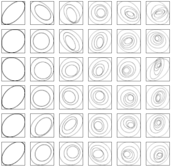
Figure 1: Sample of the artificial nested ellipses datasets. First column is taken from the first dataset with 1 ellipse, second columns from the second dataset with 2 nested ellipses, until the sixth column with 6 nested ellipses.

Table 1: Mean density with the number of nested ellipses. The density has been calculated by averaging the ratio of non-null pixel per images over 100 generated pictures for each dataset sharing the same number $n_{ellipses}$ of nested ellipses.

$n_{ellipses}$	1	2	3	4	5	6
$Density$ ($\%$)	29.0	51.4	64.3	70.9	73.5	75.0

In this first experiments we analyze the impact over MAM caused by the sparsity and number of measures. We have set $\rho=100$ without proper tuning for every dataset. The study has been carried out with one processor to avoid CPU communication management.

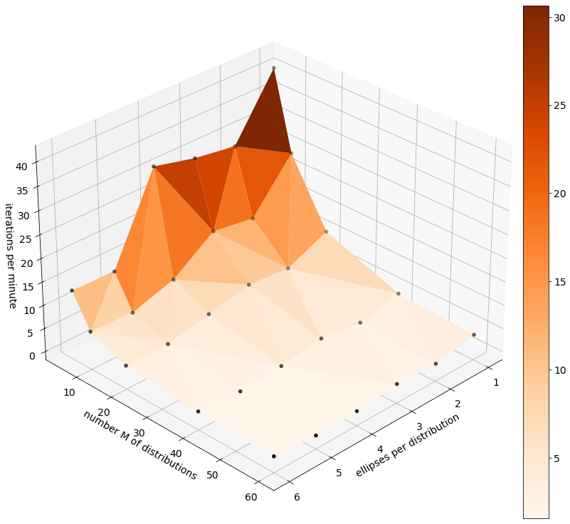
Figure 2: Evolution of the number of iterations per minute depending on the density or the number of distributions.

fig. 2 shows that, as expected, the execution time of an iteration increases with increasing density and number of measures. When compared to density it can be seen that the number of measures has greater influence on the method’s speed (such a phenomenon can be due to the $numpy$ matrix management). This means the quantity of information in each measure does not seem to make the algorithm less efficient in term of speed. Such a result is to be put in regard with algorithms such as B-ADMM [35] that are particularly shaped for sparse dataset but less efficient for denser ones. This is a significant point that will be further developed in section 6.2.3.

6.2 Comparison with IBP

The Iterative Bregman Projection (IBP) [4] is a state-of-the-art algorithm for computing Wasserstein barycenters. As mentionned in the Introduction, IBP employes a regularizing function parametrized by $\lambda>0$. The greater the $\lambda$, the worst the approximation. But in practice, $\lambda$ has to be kept in a moderate magnitude to avoid numerical errors (double-precision overflow). IBP is very sensitive to $\lambda$, that strongly relies on the dataset at stake. Thus IBP is an inexact method, whereas MAM is exact. Although the study below shows certain advantages of MAM, we make it clear that the aim is not to demonstrate which algorithm is better in general but instead to highlight the differences between the two methods and their advantages depending on the use. Note that the code for IBP is inspired from the original [21].

6.2.1 Qualitative comparison

Here we use 100 images per digit of the MNIST database [29] where each digit has been randomly translated and rotated. Each image has 40 $\times$ 40 pixels and can be treated as probability distributions thanks to a normalization, where the pixel location is the support and the pixel intensity the probability. In fig. 3, we display intermediate barycenter solutions for digits $3,4,5$ at different time steps both for MAM and IBP. For the two methods the hyperparameters have been tuned: for instance, $\lambda=1700$ is the greatest lambda that enables IBP to compute the barycenter of the 3’s dataset without double-precison overflow error. Regarding MAM, a range of values for $\rho>0$ have been tested for 100 seconds of execution, to identify which one provides good performance (for example, $\rho=50$ for the dataset of $3$’s).

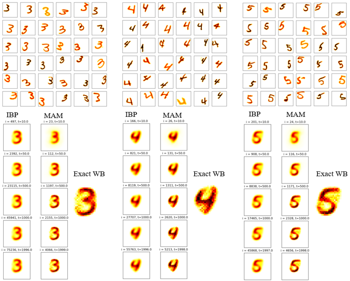
Figure 3: (top) For each digit 36 out of the 100 scaled, translated and rotated images considered for each barycenter. (bottom) Barycenters after $t=10,50,500,1000,2000$ seconds, where the left-hand-side is IBP evolution of its barycenter approximation, the middle panel is MAM evolutions using 10 CPU and the right-hand-side is the exact solution computed by applying Gurobi to the LP eq. 7.

As illustrated in fig. 3, for each dataset, IBP gets quickly to a stable approximation of a barycenter. Such a point is obtained shortly after with MAM (less than 5 to 10 seconds after) but MAM continues to converge toward a sharper solution (closer to the exact solution as exemplified quantitatively in section 6.2.2). It is clear that the more CPUs used for MAM the better. We have limited the study to a dozen of CPU to allow the reader to reproduce the experimentations. While IBP is not well shaped for CPU parallelization [21, 4, 35], MAM offers a clear advantage depending on the hardware at stake.

6.2.2 Quantitative comparison

Next we benchmark MAM, randomized MAM and IBP on a dataset with 60 images per digit of the MNIST database [29] where every digit is a normalized image 40 $\times$ 40 pixels. First, all three methods have their hyperparameters tuned thanks to a sensitivity study as explained in section 6.2.1. Then, at every time step an approximation of the computed barycenter is stored, to compute the error $\bar{W}_{2}^{2}(p^{k})-\bar{W}_{2}^{2}(p_{exact}):=\sum_{m=1}^{M}\frac{1}{M}{\tt OT}(p^{k},q^{(m)})-\sum_{m=1}^{M}\frac{1}{M}{\tt OT}(p_{exact},q^{(m)})$. All methods were implemented in $python$ using a MPI based parallelization. Note that IBP is inspired from the code of G. Peyré [21], MAM from algorithm 1 and MAM-randomized (remark 2) has only one distribution treated by processor. fig. 4 displays the evolution w.r.t time, of the error measure $\bar{W}_{2}^{2}(p^{k})-\bar{W}_{2}^{2}(p_{exact})$, with $p_{exact}$ an exact barycenter obtained by solving LP eq. 7 directly.

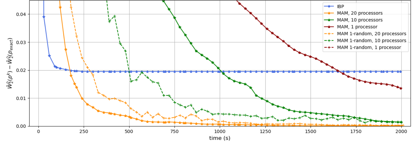
Figure 4: Evolution with respect to time of the difference between the Wasserstein barycenter distance of an approximation, $\bar{W}_{2}^{2}(p^{k})$, and the Wasserstein barycentric distance of the exact solution $\bar{W}_{2}^{2}(p_{exact})$ given by the LP. The time step between two points is 30 seconds.

It is clear that IBP is almost 10 time faster per iteration. However IBP computes an exact solution of an approximated problem that is tuned through the hyperparameter $\lambda$ (see [4]). Therefore it is natural to witness IBP converging to a solution to the approximated problem, but not to an exact WB. While MAM does converge to an exact solution. So there is a threshold where the accuracy of MAM exceeds IBP: in our case, around 200s - for the computation with the greatest number of processors (see fig. 4). Such a treshold always exists depending on the computational means (hardware).
This quantitative study explains what have been exemplified with the images of section 6.2.1: the accuracy of IBP is bounded by the choice of $\lambda$, itself bounded by an overflow error, while MAM hyperparameters only impact the convergence speed and the algorithm is always improving towards an exact solution. For this dataset, the WB computed by IBP is within 2$\%$ of accuracy and thus reasonably good. However, as shown in Table 1 in [35], one can choose other datasets where IBP’s accuracy might be unsatisfactory.

Furthermore, fig. 4 exemplifies an interesting asset of randomized variants of MAM: for some configurations randomized-MAM is more efficient than (deterministic) MAM but for others, the latter seems to be more effective. Note that the curve MAM 1-random, 1 processor does not appear on the figure: this is because it is above the y-axis value range due to its bad performance. Indeed, there is a trade-off between time spent per iteration and precision gained after an iteration. For example, with 10 processors, each processor treats 6 measures in the deterministic MAM but only one is treated in the randomized MAM. Therefore, the time spent per iteration is roughly six time shorter in the latter and this counterbalances the loss of accuracy per iterations. On the other hand, when using 20 processors, only 3 measures are treated by each processor and the trade-off is not worth it anymore: the gain in time does not compensate for the loss in accuracy per iteration. One should adapt the use of the algorithm with care since this trade-off conclusion is only heuristic and strongly depends on the dataset and hardware at use. A sensitivity analysis is always a good thought for choosing the most effective amount of measures handled per processor while using the randomized-MAM against the deterministic MAM.

6.2.3 Influence of the support

This section is echoing section 6.1 and studies the influence of the support size. To do so, two datasets have been tested for MAM and IBP. The first dataset is already used in section 6.2.2: 60 pictures of 3’s taken from the classic MNIST database [29]. The second dataset is also composed by these 60 images but each digit has been randomly translated and rotated in the same way as in fig. 3. Therefore, the union of the support of the second dataset is greater than the first one, as illustrated in fig. 5.

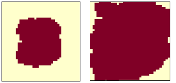
Figure 5: Images with $40\times 40$ pixel grid, where the red represents the pixels which are in the union of the dataset support composed with 60 images. (left) for the standard MNIST, (right) for the randomly translated and rotated MNIST.

fig. 6 presents two graphs that have been obtained just as in section 6.2.2, but displaying the evolution w.r.t time in percentage: $\Delta W_{\%}:=\frac{\bar{W}_{2}^{2}(p^{k})-\bar{W}_{2}^{2}(p_{exact})}{\bar{W}_{2}^{2}(p_{exact})}\times 100$. Once more, the hyperparameters have been fully tuned. The hyperparameter of the IBP method is smaller for the second datacase. Indeed, as stated in [35], the greater is the support, the stronger are the restrictions on $\lambda$. And since the smaller is $\lambda$ the further is the approximated problem to the exact one this is expected to witness rising differences between on the following graphs.

Figure 6: Evolution of the percentage of the distance between the exact solution of the barycenter problem and the computed solution using IBP and MAM method with 20 processors: (left) for the standard MNIST, (right) for the randomly translated and rotated MNIST.

Being an exact method, MAM is insensitive to support size. The density of the dataset has little impact on the convergence time as explained in section 6.1 and exemplified in fig. 6. Such visual results concerning IBP initialization and parametrization have already been discussed in fig. 3, some other qualitative results can be found in [24] where the author shows that properties of the distributions can be lost due to the entropy penalization in IBP.

6.3 Comparison with B-ADMM

This subsection compares MAM with the algorithm B-ADMM of [31] using the dataset and Matlab implementation provided by the authors at the link https://github.com/bobye/d2_kmeans. We omit IBP in our analysis because it has already been shown in [31, Table I] that IBP is outperformed by B-ADMM in this dataset. As in [31, Section IV], we consider $M=1000$ discrete measures, each with a sparse finite support set obtained by clustering pixel colors of images. The average number of support points is around $6$, and the barycenter’s number of (fixed) support points is $R=60$. An exact WB can be computed by applying an LP solver to the extensive formulation eq. 7. Its optimal value is $712.7$, computed in $10.6$ seconds by the Gurobi LP solver. We have coded MAM in Matlab to have a fair comparison with the Matlab B-ADMM algorithm provided at the above link. Since MAM and B-ADMM use different stopping tests, we have set their stopping tolerances equal to zero and let the solvers stop with a maximum number of iterations. Table 2 below reports CPU time in seconds and the objective values yielded by the (approximated) barycenter $\tilde{p}$ computed by both solvers: $\bar{W}_{2}^{2}(\tilde{p})$.

Table 2: MAM vs B-ADMM. The considered implementation of B-ADMM is the one provided by its designers without changing parameters (except the stopping set to zero and the maximum number of iterations). Both algorithms use the same initial point. The dataset is the one considered in [31, Section IV]. The optimal value of the WB barycenter for this dataset is $712.7$, computed by Gurobi in $10.6$ seconds.

Iterations	Objective value		Seconds
	B-ADMM	MAM	B-ADMM	MAM
100	742.8	716.7	1.1	1.1
200	725.9	714.1	2.4	2.2
500	716.5	713.3	5.6	5.4
1000	714.1	712.9	11.8	10.8
1500	713.5	712.8	18.9	16.2
2000	713.3	712.8	25.1	21.6
2500	713.2	712.8	31.0	27.1
3000	713.1	712.7	39.8	32.4

The results show that, for the considered dataset, MAM and B-ADMM are comparable regarding CPU time, with MAM providing more precise results. In contrast with MAM, B-ADMM does not have (at this time) a convergence analysis.

6.4 Unbalanced Wasserstein Barycenter

This section treats a particular example to illustrate the interest of using UWB. The artificial dataset is composed by 50 images with resolution $80\times 80$. Each image is divided in four squared. The top left, bottom left and bottom right squared are randomly filled with double nested ellipses and the top right squared is always empty as exemplified in fig. 7. In this example, every image is normalized to depict a probability measure so that we can compare WB and UWB.

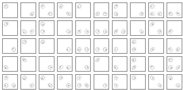
Figure 7: Dataset composed by 50 pictures with nested ellipses randomly positionned in the top left, bottom right and left corners.

With respect to eq. 10, one set of constraints is relaxed and the influence of the hyperparameter $\gamma$ is studied. If $\gamma$ is large enough (i.e. greater than $\Arrowvert{\tt vec}(d)\Arrowvert\approx 1000$, see proposition 1), the problem boils down to the standard WB problem since the example deals with probability measures: the resulting UWB is indeed a WB. When decreasing $\gamma$ the transportation costs take more importance than the distance to $\mathcal{B}$ that is more and more relaxed. Therefore, as illustrated by fig. 8, the resulting UWB splits the image in four parts, giving visual meaning to the barycenter.

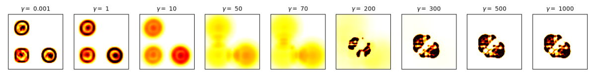
Figure 8: UWB computed with MAM for different values of $\gamma$.

In the same vein, fig. 9 provides an illustrative application of MAM for computing UWB in another dataset.

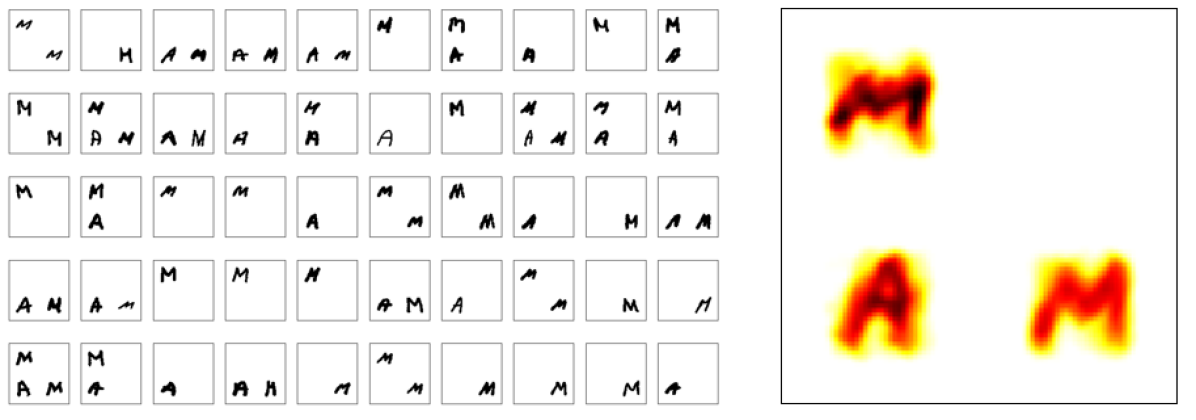
Figure 9: (left) UWB for a dataset of letters M-A-M built in the same logic than fig. 7 with 50 figures: (right) resulting UWB with $\gamma=0.01$, computed in 200 seconds using 10 processors.

References

- [1] Martial Agueh and Guillaume Carlier. Barycenters in the wasserstein space. Siam Journal on Mathematical Analysis, 43(2):904–924, 2011.
- [2] Gilles Bareilles, Yassine Laguel, Dmitry Grishchenko, Franck Iutzeler, and Jérôme Malick. Randomized progressive hedging methods for multi-stage stochastic programming. Annals of Operations Research, 295(2):535–560, sep 2020.
- [3] Heinz H. Bauschke and Patrick L. Combettes. Convex Analysis and Monotone Operator Theory in Hilbert Spaces. Springer International Publishing, 2nd edition, 2017.
- [4] Jean-David Benamou, Guillaume Carlier, Marco Cuturi, Luca Nenna, and Gabriel Peyré. Iterative bregman projections for regularized transportation problems. SIAM Journal on Scientific Computing, 37(2):1111–1138, 2015.
- [5] Dimitri P. Bertsekas. Convex Optimization Algorithms. Number 1st. Athena Scientific, 2015.
- [6] Steffen Borgwardt. An lp-based, strongly-polynomial 2-approximation algorithm for sparse wasserstein barycenters. Operational Research, 22(2):1511–1551, Apr 2022.
- [7] Guillaume Carlier, Adam Oberman, and Edouard Oudet. Numerical methods for matching for teams and wasserstein barycenters. ESAIM: Mathematical Modelling and Numerical Analysis, 49(6):1621–1642, nov 2015.
- [8] Laurent Condat. Fast projection onto the simplex and the ball. Mathematical Programming, 158(1):575–585, Jul 2016.
- [9] Marco Cuturi. Sinkhorn distances: Lightspeed computation of optimal transport. In C.J. Burges, L. Bottou, M. Welling, Z. Ghahramani, and K.Q. Weinberger, editors, Advances in Neural Information Processing Systems, volume 26. Curran Associates, Inc., 2013.
- [10] Marco Cuturi and Arnaud Doucet. Fast computation of wasserstein barycenters. In Eric P. Xing and Tony Jebara, editors, Proceedings of the 31st International Conference on Machine Learning, volume 32 of Proceedings of Machine Learning Research, pages 685–693, Bejing, China, 22–24 Jun 2014. PMLR.
- [11] Marco Cuturi and Arnaud Doucet. Fast computation of wasserstein barycenters. International Conference on Machine Learning, 32(2):685–693, 2014.
- [12] Marco Cuturi and Gabriel Peyré. A smoothed dual approach for variational wasserstein problems. SIAM Journal on Imaging Sciences, 9(1):320–343, 2016.
- [13] Welington de Oliveira, Claudia Sagastizábal, Débora Dias Jardim Penna, Maria Elvira Pineiro Maceira, and Jorge Machado Damázio. Optimal scenario tree reduction for stochastic streamflows in power generation planning problems. Optimization Methods and Software, 25(6):917–936, 2010.
- [14] Jim Douglas and H. H. Rachford. On the numerical solution of heat conduction problems in two and three space variables. Transactions of the American Mathematical Society, 82(2):421–439, 1956.
- [15] Jonathan Eckstein and Dimitri P. Bertsekas. On the douglas—rachford splitting method and the proximal point algorithm for maximal monotone operators. Mathematical Programming, 55(1-3):293–318, apr 1992.
- [16] Anqi Fu, Junzi Zhang, and Stephen Boyd. Anderson accelerated douglas–rachford splitting. SIAM Journal on Scientific Computing, 42(6):A3560–A3583, jan 2020.
- [17] A. Gramfort, G. Peyré, and M. Cuturi. Fast optimal transport averaging of neuroimaging data. In Sebastien Ourselin, Daniel C. Alexander, Carl-Fredrik Westin, and M. Jorge Cardoso, editors, Information Processing in Medical Imaging, pages 261–272, Cham, 2015. Springer International Publishing.
- [18] Tartavel Guillaume, Peyré Gabriel, and Gousseau Yann. Wasserstein loss for image synthesis and restoration. SIAM Journal on Imaging Sciences, 9(4):1726–1755, 2016.
- [19] Florian Heinemann, Marcel Klatt, and Axel Munk. Kantorovich–rubinstein distance and barycenter for finitely supported measures: Foundations and algorithms. Applied Mathematics & Optimization, 87(1):4, Nov 2022.
- [20] Franck Iutzeler, Pascal Bianchi, Philippe Ciblat, and Walid Hachem. Asynchronous distributed optimization using a randomized alternating direction method of multipliers. In 52nd IEEE Conference on Decision and Control. IEEE, dec 2013.
- [21] Gabriel Peyré. Bregmanot, 2014.
- [22] Gabriel Peyré and Marco Cuturi. Computational optimal transport: With applications to data science. Foundations and Trends in Machine Learning, 11(5-6):355–607, 2019.
- [23] Georg Ch. Pflug and Alois Pichler. Multistage Stochastic Optimization. Springer International Publishing, 2014.
- [24] Giovanni Puccetti, Ludger Rüschendorf, and Steven Vanduffel. On the computation of wasserstein barycenters. Journal of Multivariate Analysis, 176(104581), 2020.
- [25] Yossi Rubner, Carlo Tomasi, and Leonidas J. Guibas. The earth mover’s distance as a metric for image retrieval. International Journal of Computer Vision, 40(2):99–121, Nov 2000.
- [26] Thibault Sejourne, Gabriel Peyre, and Francois-Xavier Vialard. Unbalanced optimal transport, from theory to numerics. Handbook of Numerical Analysis, 24:407–471, 2023.
- [27] Dror Simon and Aviad Aberdam. Barycenters of natural images constrained wasserstein barycenters for image morphing. In Proceedings of the IEEE/CVF Conference on Computer Vision and Pattern Recognition, pages 7910–7919, 2020.
- [28] Richard Sinkhorn. Diagonal equivalence to matrices with prescribed row and column sums. ii. Proceedings of the American Mathematical Society, 45(2):195–198, 1974.
- [29] Tijmen. affnist, 2013.
- [30] Cedric Villani. Optimal transport: onld and new, volume 338. Springer Verlag, 2009.
- [31] Huahua Wang and Arindam Banerjee. Bregman alternating direction method of multipliers. In Z. Ghahramani, M. Welling, C. Cortes, N. Lawrence, and K.Q. Weinberger, editors, Advances in Neural Information Processing Systems, volume 27. Curran Associates, Inc., 2014.
- [32] Jean-Paul Watson and David L. Woodruff. Progressive hedging innovations for a class of stochastic mixed-integer resource allocation problems. Computational Management Science, 8(4):355–370, jul 2010.
- [33] Zheng Xu, Mario Figueiredo, and Tom Goldstein. Adaptive ADMM with Spectral Penalty Parameter Selection. In Aarti Singh and Jerry Zhu, editors, Proceedings of the 20th International Conference on Artificial Intelligence and Statistics, volume 54 of Proceedings of Machine Learning Research, pages 718–727. PMLR, 20–22 Apr 2017.
- [34] Jianbo Ye and Jia Li. Scaling up discrete distribution clustering using ADMM. In 2014 IEEE International Conference on Image Processing (ICIP), pages 5267–5271, 2014.
- [35] Jianbo Ye, Panruo Wu, James Z. Wang, and Jia Li. Fast discrete distribution clustering using wasserstein barycenter with sparse support. IEEE Transactions on Signal Processing, 65:2317–2332, May 2017.