Unified tensor network theory for frustrated classical spin models in two dimensions

Abstract

Frustration is a ubiquitous phenomenon in many-body physics that influences the nature of the system in a profound way with exotic emergent behavior. Despite its long research history, the analytical or numerical investigations on frustrated spin models remain a formidable challenge due to their extensive ground state degeneracy. In this work, we propose a unified tensor network theory to numerically solve the frustrated classical spin models on various two-dimensional (2D) lattice geometry with high efficiency. We show that the appropriate encoding of emergent degrees of freedom in each local tensor is of crucial importance in the construction of the infinite tensor network representation of the partition function. The frustrations are thus relieved through the effective interactions between emergent local degrees of freedom. Then the partition function is written as a product of a one-dimensional (1D) transfer operator, whose eigen-equation can be solved by the standard algorithm of matrix product states rigorously, and various phase transitions can be accurately determined from the singularities of the entanglement entropy of the 1D quantum correspondence. We demonstrated the power of our unified theory by numerically solving 2D fully frustrated XY spin models on the kagome, square and triangular lattices, giving rise to a variety of thermal phase transitions from infinite-order Brezinskii-Kosterlitz-Thouless transitions, second-order transitions, to first-order phase transitions. Our approach holds the potential application to other types of frustrated classical systems like Heisenberg spin antiferromagnets.

I Introduction

Frustrated spin systems have become an extremely active field of theoretical and experimental research in the last decades characterized by complex low-energy physics and fascinating emergent phenomenaLacroix et al. (2011); Ramirez (1994); Moessner (2001). A system is regarded as frustrated when conflicting interaction terms are present, featured by the inability to minimize total energy by concurrently reducing the energy of each group of interacting degrees of freedom. Frustration underlies non-trivial behavior across physical systems or more general many-body systems, as the minimization of local conflicts gives rise to new degrees of freedomDiep (2020); Ortiz-Ambriz et al. (2019).

Classical frustrated spin systems can be understood as simplified quantum mechanical models which employ classical spins to investigate the behavior of strongly correlated magnetic systems with competing interactions. The existence of frustration depends on the lattice geometry and/or the nature of the interactionsSadoc and Mosseri (1999). For example, the anti-ferromagnetic (AF) Ising model defined by a set of spins of $s=\pm 1$ is frustrated on the triangular and kagome lattices with massive ground-state degeneracyWannier (1950); Kanô and Naya (1953). However, AF Ising models are not frustrated on the 2D square lattice because the lattice is bipartite and the energy can be simply minimized by the Neel configuration of alternating spins. Frustration also depends on the dimension of the spin variables. For the frustrated AF XY spin systems composed of planar vectors $\vec{s}=(\sin\theta,\cos\theta)$, the ground-state configuration is usually highly degenerate with new symmetries induced from non-collinear patterns. The new degrees of freedom can give rise to rich and complex phases at finite temperatures, which have been studied over the past decades on the squareTeitel and Jayaprakash (1983); Thijssen and Knops (1990); Ramirez-Santiago and José (1992); Granato and Nightingale (1993); Lee (1994); Lee and Lee (1994); Ramirez-Santiago and José (1994); Olsson (1995); Cataudella and Nicodemi (1996); Olsson (1997); Boubcheur and Diep (1998); Hasenbusch et al. (2005); Okumura et al. (2011); Nussinov (2014); Lima et al. (2019); Song and Zhang (2022), the triangular Miyashita and Shiba (1984); Shih and Stroud (1984); Lee et al. (1984, 1986); Korshunov and Uimin (1986); Van Himbergen (1986); Xu and Southern (1996); Lee and Lee (1998); Capriotti et al. (1998) and the kagome lattices Harris et al. (1992); Rzchowski (1997); Cherepanov et al. (2001); Park and Huse (2001); Korshunov (2002); Andreanov and Fistul (2020); Song and Zhang (2023).

The study of frustrated classical spin systems is important not only for understanding the emergent behavior of physical systems like spin glassesVillain (1977a); Binder and Young (1986) but also for general optimization problems across multiple disciplinesHartmann and Rieger (2001). Considerable efforts have been made in the investigation of the fundamental properties of frustrated classical spin systems. Despite decade-long efforts, a generic approach to dealing with frustrated spin systems with both high accuracy and high efficiency is still lacking. Well-established methods such as Monte Carlo simulations, mean-field theories, and renormalization group techniques, have made significant contributions to the study of the classical frustrated spin models. However, they have encountered many difficulties such as low efficiency or limited applicationsSwendsen and Wang (1987); Wolff (1989); Rakala and Damle (2017); Andreanov and Fistul (2020).

Recent progress in the tensor network methods provides new computational approaches for studying classical lattice models with strong frustrationsVanderstraeten et al. (2018); Vanhecke et al. (2021); Song and Zhang (2022); Colbois et al. (2022); Song and Zhang (2023). It is found that the construction of the tensor network of the partition function is nontrivial for frustrated systems compared to the standard formulation. For example, the ground state local rules should be encoded in the local tensors to satisfy the ground state configurations induced by geometrical frustrationsVanderstraeten et al. (2018). In the frustrated Ising models, a linear searching algorithm based on a Hamiltonian tessellation has been proposed to find the proper transitional invariant unitVanhecke et al. (2021); Colbois et al. (2022). In the frustrated XY models, the idea of splitting of $U(1)$ spins and dual transformations have been developed to overcome the convergence issuesSong and Zhang (2022, 2023). Although these techniques make a success in specific models, they seem to be very tricky. Thus, one wonders whether there exists a general framework to treat frustrated classical spin models.

Here, we generalize the underlying principles of the tensor network representation to make it applicable to generic frustrated classical spin systems. When comprising the whole tensor network of the partition function, the crucial point is that the emergent degrees of freedom induced by frustrations should be encoded in the local tensors. In this way, the massive degeneracy is characterized by emergent dual variables such as height variables in the AF Ising model on the triangular latticeBlote and Hilborst (1982); Chalker (2017) and chiralities in frustrated XY modelsKorshunov (2002); Song and Zhang (2023). The emergent variables capture the freedom of a group of interacting spins under the constraint of frustrations. In the sense of coarse-graining, the local tensors carry the effective interactions between emergent local degrees of freedom. The local tensors usually sit on the dual sites of the original lattice which can be constructed from dual transformations. It is worth noting that the dual transformations should be imposed on the whole cluster of a number of spins in correspondence with the emergent dual variables.

We demonstrate the power of the generalized theory of tensor network representation by applying it to fully frustrated XY models on the kagome, triangular, and square lattices. First of all, we can express the infinite 2D tensor network as a product of 1D transfer matrix operators, which can be contracted efficiently by recently developed tensor network algorithms under optimal variational principlesZauner-Stauber et al. (2018); Vanderstraeten et al. (2019a); Nietner et al. (2020). Then, from the singularity of the entanglement entropy of the 1D quantum transfer operator, various phase transitions can be determined with great accuracy according to the same criterionHaegeman and Verstraete (2017). Finally we find that a broad array of emergent physics has been treated including various types of phase transitions from first-order, second-order to the Berezinskii-Kosterlitz-Thouless (BKT) phase transitions. The complex phase structures of the frustrated XY systems are revisited and clarified with new tensor network solutions. The present approach holds the potential application to next-nearest-neighbor frustrated spin systems and other types of classical spins like Heisenberg antiferromagnet.

The rest of the paper is organized as follows. In Sec. II, we introduce the theory of tensor network representations for classical frustrated spin models with two concrete examples. After constructing the tensor networks of Ising spin antiferromagnets on the kagome and triangular lattices, we perform the numerical calculation of the residual entropy of the frustrated Ising models, which are comparable to the exact results. In Sec. III, we apply the unified theory to the fully frustrated XY spin models on the kagome, square, and triangular lattices, and present the numerical results for the determination of the finite temperature phase diagram of frustrated XY systems, especially the AF triangular XY model and the modified square XY model. Finally in Sec. IV, we discuss the future generalizations of the method and give our conclusions. In the Appendix, we outline the detailed tensor network methods for numerical calculations.

II Tensor network representations of 2D statistical models

II.1 Emergent degrees of freedom

Tensor networks have proven to be a very potent tool in the study of strongly correlated quantum models as well as classical statistical mechanics. To implement this powerful method, the first step is to convert the partition function of a classical lattice model with local interactions into a tensor network representation.

The standard construction of the tensor network is conducted by putting a matrix on each bond of the original lattice accounting for the Boltzmann weight of the nearest-neighboring interactionsZhao et al. (2010). For a generic spin model with nearest-neighbor interactions

$$H=\sum_{\langle i,j\rangle}h(s_{i},s_{j}),$$ (1)

the partition function can be decomposed into a tensor network as a product of local Boltzmann weights,

$$Z=\sum_{\{s_{i}\}}\mathrm{e}^{-\beta H(\{s_{i}\})}=\sum_{\{s_{i}\}}\prod_{\langle i,j\rangle}W(s_{i},s_{j}),$$ (2)

where $\langle i,j\rangle$ refers to the nearest neighbors, $s_{i}$ are the spin variables, and the interaction matrices are given by

$$W(s_{i},s_{j})=\mathrm{e}^{-\beta h(s_{i},s_{j})},$$ (3)

whose row and column indices are the spin variables shown in Fig. 1. The $\delta$ tensors on the lattice vertexes ensure all indices of $W$ take the same value at the joint point.

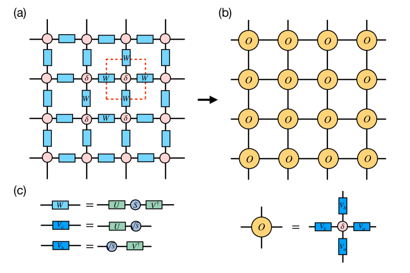
Figure 1: The standard construction of the tensor network. (a) The $W$ matrix represents the Boltzmann weight on each link, and the $\delta$ tensor on each site represents the sharing of the same spin between neighboring $W$ matrices. (b) The tensor network representation of the partition function composed of uniform local tensors. (c) The local tensor $O$ is built by the singular value decomposition (SVD) on each $W$ matrix and the grouping of the $V$ matrices connecting to the $\delta$ tensors.

Furthermore, we perform the Schmidt decomposition on the symmetric matrix $W$

$$W(s_{i},s_{j})=(U\sqrt{S})(\sqrt{S}V^{\dagger})=V_{a}(s_{i},s_{k})V_{b}(s_{k},s_{j}),$$ (4)

and the partition function can be cast into the uniform tensor network representation as shown in Fig. 1

$$Z=\mathrm{tTr}\prod_{i}O_{s_{1},s_{2}}^{s_{3},s_{4}}(i)$$ (5)

by grouping all V matrices that connect to the $\delta$ tensors

$$O_{s_{1},s_{2}}^{s_{3},s_{4}}=\sum_{s_{k}}V_{b}(s_{1},s_{k})V_{b}(s_{2},s_{k})V_{a}(s_{k},s_{3})V_{a}(s_{k},s_{4}).$$ (6)

The standard representation has been successfully applied to many lattice statistical models without frustrationLevin and Nave (2007); Zhao et al. (2010); Yu et al. (2014); Haegeman and Verstraete (2017); Vanderstraeten et al. (2019b). However, it cannot be implemented directly in the frustrated spin models, where the tensor network contraction algorithms fail to converge. It was found that the proper encoding of the ground state local rules in local tensors was crucial for the contraction to converge. To fulfill the physics of the ground state manifold, a linear algorithm was proposed to search for the optimal Hamiltonian tessellation for Ising antiferromagnetsVanhecke et al. (2021); Colbois et al. (2022). The key point is that the energy of all local ground state configurations should be simultaneously minimized under the splitting of the global Hamiltonian into local groups of interactions. And the local tensors are constructed as translational units coinciding with the local clusters of the tessellation.

In order to extend tensor network approaches to generic frustrated classical spin models, we should understand the ground state local rules from a more fundamental perspective of emergent degrees of freedom. In frustrated systems, new degrees of freedom often emerge as a result of the minimization of local conflicts. The ground state of frustrated spin systems is highly degenerate because a number of spins can behave as free spins. Such freedom can therefore be represented by a set of emergent variables describing the effective interactions induced by frustrations. For some models, the emergent variables can be derived directly like height variables in the AF Ising triangular modelBlote and Hilborst (1982); Chalker (2017) and chiralities in frustrated XY modelsKorshunov (2002); Song and Zhang (2023). For the spin models with more complicated interactions, the emergent variables may not be explicitly expressed but they can still be characterized by local tensors composed of a cluster of local interactionsVanhecke et al. (2021); Colbois et al. (2022). This idea generalizes tensor network approaches readily to classical frustrated systems of both discrete and continuous spins.

Before discussing the tensor network construction of the frustrated spin model, we give some examples of emergent degrees of freedom by revisiting the exactly solvable frustrated models. One of the simplest frustrated spin models is the AF Ising model on the kagome lattice

$$H=J\sum_{\langle i,j\rangle}\sigma_{i}\sigma_{j},$$ (7)

where $J>0$ denotes the AF interactions between nearest-neighbor spins $s_{i}=\pm 1$ as displayed in Fig. 2 (a).

The kagome AF Ising model is disordered at all temperatures with an extensive ground state degeneracy characterized by a finite residual entropyKanô and Naya (1953). To minimize the energy of each triangular plaquette, three spins should obey the ground state local rule of “two up one down, one down two up” as shown in Fig. 2 (a).

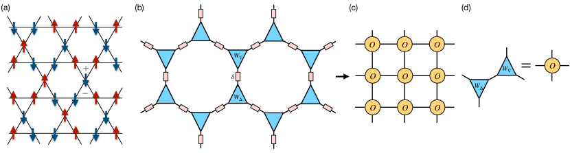
Figure 2: Tensor network representation of the AF Ising model on a kagome lattice. (a) One of the ground state configurations on the kagome lattice with $Q=\pm 1$ charges on each triangle. (b) Putting the $W_{\Delta}$ ($W_{\nabla}$) tensors on the centers of the upward (downward) triangles to represent the self-energy of the charge variables, where the $\delta$ tensors between the nearest neighbor triangles can be translated into the connections of tensor legs directly. (c) The tensor network representation of the partition function composed of uniform local $O$ tensors. (d) The construction of $O$ tensor by contracting neighboring $W_{\Delta}$ and $W_{\nabla}$ tensors.

Besides directly focusing on the local spin configurations, the physics of the model can be understood from the emergent degrees of freedom on the triangle centers. A set of charge variables can be defined at each triangle

$$Q_{u}=\sum_{i\in\Delta}s_{i},\quad Q_{d}=-\sum_{i\in\nabla}s_{i},$$ (8)

where $\Delta$ and $\nabla$ denote the upward and downward triangles. The Hamiltonian can then be expressed as

$$H=\frac{J}{2}\sum_{p\in\Delta(\nabla)}(Q_{p}^{2}-3)$$ (9)

in terms of the topological charges $Q_{p}$.

Although there seems to be no explicit interaction between charges in the Hamiltonian, the variables $Q_{p}$ are not independent because the shared spin between the neighboring triangles should be the same. The constraints between neighboring charges can be naturally represented by a link between local tensors as a Kronecker delta tensor in the language of tensor networks. In this way, the interactions between Ising spins are transformed into a charge model including the self-energy of the charges and the effective interactions between these charges. The charge variables can take four values $Q=\pm 1,\pm 3$ at finite temperatures. In the zero temperature limit, the charges of $Q=\pm 3$ are energetically suppressed. The “two up one down, one up two down” rule corresponds to charge variables $Q=\pm 1$ allowed by the ground state manifold.

The emergent charge variables can also be applied to the triangular lattice in the same spirit as the case of the kagome lattice. The triangular AF Ising model in Fig. 3 (a) can be transformed into

$$H=\frac{J}{2}\sum_{\langle i,j\rangle\in p}s_{i}s_{j}=\frac{J}{4}\sum_{p}\left(Q_{p}^{2}-3\right),$$ (10)

where the only difference is that each nearest-neighbor triangles share two same spins. The charges variables help us to understand why the tiling of $p\in\Delta(\nabla)$ is crucial for the triangular latticesVanhecke et al. (2021). The reason is that the tessellation of only one type of triangle fails to characterize the interactions between the emergent charge variables.

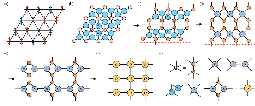
Figure 3: Tensor network representations of the Ising anti-ferromagnet on a triangular lattice. (a) One of the massive degenerate ground state configurations. (b) The $W_{\nabla}$ and $W_{\Delta}$ tensors are defined on the center of the triangles. The pink $\delta$ tensor represents a six-legged Kronecker delta tensor which connects the $W_{\nabla}$ and $W_{\Delta}$ tensors surrounding it. (c)-(d) The construction of row-to-row transfer matrix by splitting the six-legged $\delta$ tensors vertically and regrouping the index of a pair of neighboring $W_{\nabla}$ and $W_{\Delta}$ tensor into an $I^{\prime}$ tensor. (e)-(f) The construction of the local uniform tensor O by splitting $I^{\prime}$ horizontally and grouping with $\delta^{u}$ and $\delta^{d}$ tensors. (g) The details of the operations on local tensors during the construction procedure.

II.2 General principle for tensor network construction

Now we can build up a general principle for the tensor network representation of frustrated spin models. The key point is that the emergent degrees of freedom should be encoded in each local tensor in the construction of the infinite tensor network for the partition function. Since the emergent degrees of freedom is universal in frustrated systems, the generic approach can be applied to classical frustrated systems of both discrete and continuous symmetries. Moreover, the finite-temperature properties can also be probed when the interactions among emergent degrees of freedom are faithfully captured.

In practice, it is not necessary to write down the explicit model of the interactions between emergent variables. The effective interactions are implicit in the connections between local tensors. Each local tensor constituting the Boltzmann weight should carry the emergent degrees of freedom corresponding to a unit cluster of spins. From this perspective, the breakdown of standard construction in the triangular Ising modelVanhecke et al. (2021) can be understood: the emergent degrees of freedom located on the downward triangles are lost in the infinite tensor network contraction.

We summarize the general procedure to construct the tensor network representation of the frustrated spin models as follows:

i). Identify the emergent degree of freedom, usually located on the dual site, and the corresponding geometry cluster composed of classical spins.

ii). Reformulate the partition function into the form of

$$Z=\sum_{\{s\}}\prod_{c}W_{c}(c)\prod_{\langle c,c^{\prime}\rangle}W_{l}(c,c^{\prime})\delta_{c,c^{\prime}}$$ (11)

where $c$ enumerates all the clusters, $W_{c}$ and $W_{l}$ correspond to the Boltzmann weight of all the spin configurations $\{s\}$ within a cluster and between neighboring clusters, and $\delta$ tensors ensure the shared spins between different clusters be the same. For continuous spins, the $W$ tensors should be transformed onto a discrete basis via the Fourier transformation.

iii). Split and regroup the $W$ tensors to build regular local tensors constituting an infinite uniform tensor network representation of the partition function.

II.3 Kagome and triangular AF Ising models as two examples

The general principle can be applied directly to classical frustrated models with discrete symmetries. The tensor network representation of the kagome AF Ising model (7) can be built simply based on the emergent charge variables defined in (8). As displayed in Fig. 2 (b), we first split the global Boltzmann weight into local Boltzmann weights on each triangle. Then the partition function of the AF Ising model can be written as

$$Z=\sum_{\{s_{i}\}}\prod_{p}W_{p}(s_{1},s_{2},s_{3}),$$ (12)

where the Boltzmann weight on each upward and downward triangle is expressed by a three-legged $W$ tensor

$$W_{p}(s_{1},s_{2},s_{3})=\mathrm{e}^{-\beta J(s_{1}s_{2}+s_{2}s_{3}+s_{3}s_{1})}.$$ (13)

The constraint of sharing the same spin between a pair of neighboring $W$ tensors is imposed by the Kronecker delta tensor.

Then the transitional invariant local tensor $O$ is achieved by combining a pair of upward and downward triangles

$$O_{s_{1},s_{2}}^{s_{3},s_{4}}=\sum_{s_{5}}W_{\Delta}(s_{1},s_{2},s_{5})W_{\nabla}(s_{5},s_{3},s_{4})$$ (14)

as displayed in Fig. 2 (d), and the uniform tensor network representation of the partition function in Fig. 2 (c) is given by

$$Z=\mathrm{tTr}\prod_{i}O_{s_{1},s_{2}}^{s_{3},s_{4}}(i)$$ (15)

where “tTr means the tensor contraction over all auxiliary links and $i$ denotes the sites of the transitional invariant unit.

The above tensor network can be contracted efficiently using standard algorithms for infinite systems with extremely high accuracyHaegeman and Verstraete (2017); Zauner-Stauber et al. (2018); Vanderstraeten et al. (2019a). In the zero temperature limit, the tensor $W$ can be reduced to the same tensor obtained in the Ref.Vanhecke et al. (2021), yielding a residual entropy of $S_{0}\approx 0.501833$, consistent with the exact resultKanô and Naya (1953).

For the triangular AF Ising model displayed in Fig. 3 (a), the tensor network representation can be constructed in a similar way. The only difference is that each spin is shared by six surrounding triangles. As shown in Fig. 3 (b), the constraint between the triangular plaquettes is realized through the six-legged delta tensors

$$\delta_{s_{1},s_{2},s_{3},s_{4},s_{5},s_{6}}=\begin{cases}1,&s_{1}=s_{2}=s_{3}=s_{4}=s_{5}=s_{6}\\ 0,&\text{otherwise}\end{cases}$$ (16)

and the tensor $W$ is defined in the same way as the kagome AF Ising model Eq. (13).

To construct a row-to-row transfer matrix, we split the six-legged delta tensors vertically as two four-legged delta tensors

$$\delta_{s_{1},s_{2},s_{3},s_{4},s_{5},s_{6}}=\sum_{s_{7}=\pm 1}\delta_{s_{1},s_{2},s_{3},s_{7}}^{u}\delta_{s_{7},s_{4},s_{5},s_{6}}^{d}$$ (17)

as shown in Fig. 3 (c). Then a pair of $W_{\Delta}$ and $W_{\nabla}$ are grouped into a tensor $I^{\prime}$ as shown in Fig. 3 (d). The tensor $I^{\prime}$ can be further split horizontally as displayed in Fig. 3 (e)

$$I^{\prime}=LR$$ (18)

by a singular-value decomposition

$$I^{\prime}=USV^{\dagger},$$ (19)

where $U$ and $V^{\dagger}$ are three-legged unitary tensors, $S$ is a semi-positive diagonal matrix and

$$L=U\sqrt{S},\quad R=\sqrt{S}V^{\dagger}.$$ (20)

Finally, the regular local tensor $O$ is obtained by grouping $\delta^{u}$, $\delta^{d}$, and a pair of $L$ and $R$ tensors. The details are depicted in Fig. 3 (g). This gives a uniform tensor-network representation of the partition function

$$Z=\mathrm{tTr}\prod_{i}O_{s_{1},s_{2}}^{s_{3},s_{4}}(i)$$ (21)

as displayed in Fig. 3 (f). Although the local tensor $O$ is slightly different from the one constructed by the method of Hamiltonian tessellationVanhecke et al. (2021), the tensor network is well defined and can be readily generalized to frustrated systems with continuous symmetries discussed in the following parts.

As shown in Fig. 4 (a), standard contraction algorithmsZauner-Stauber et al. (2018); Fishman et al. (2018); Vanderstraeten et al. (2019a) display a nice convergence at both zero temperature and finite temperatures. The numerical calculation of the expectation value of the magnetization

$$m=\langle s_{i}\rangle=\frac{1}{N}\sum_{i}s_{i}$$ (22)

is found to be zero under all temperatures, indicating the absence of the long-range order (LRO). Moreover, the ground state residual entropy is calculated as displayed in Fig. 4 (b)

$$S_{0}=\frac{1}{N}\ln Z_{0}\approx 0.323065,$$ (23)

in good agreement with the exact resultWannier (1950).

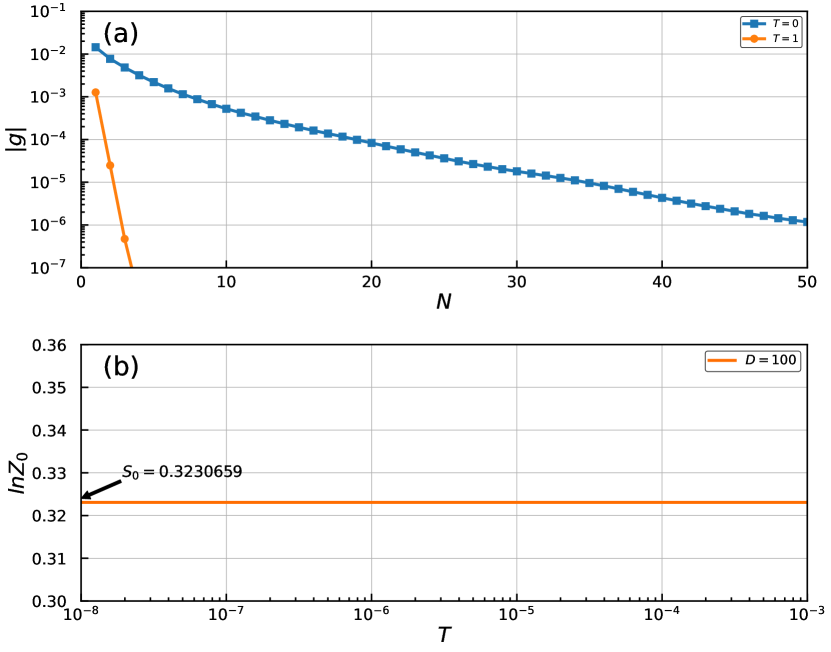
Figure 4: Numerical results of the Ising anti-ferromagnet on the triangular lattice, the bond dimension of uniform MPS is $D=100$. (a) Convergence of the VUMPS algorithm at $T=1$ and $T=0$. $|g|$ is the convergence measure in the VUMPS algorithm and $N$ is the number of iteration steps. (b) $\ln Z_{0}$ as a function of temperature. The residual entropy per site is $S_{0}(D=100)=0.3230659$, which is the same as the exact result to seven decimal places.

III Tensor network theory for 2D fully frustrated XY spin models

III.1 Duality transformation and split of $U(1)$ spins

In this section, we demonstrate the power of the generic idea of emergent degrees of freedom by the implementations in the frustrated model with a continuous $U(1)$ symmetry. The frustrated XY models, to some extent, are “less frustrated” than the Ising ones. The XY spins have more freedom to rotate on the plane to minimize local conflict interactions, but the Ising spins are constrained to only two orientations. That is why there exists quasi-LRO in the frustrated XY spin models at low temperatures, while the frustrated Ising models are usually disordered even at zero temperature. Despite a long history of investigationsTeitel and Jayaprakash (1983); Thijssen and Knops (1990); Ramirez-Santiago and José (1992); Granato and Nightingale (1993); Lee (1994); Lee and Lee (1994); Ramirez-Santiago and José (1994); Olsson (1995); Cataudella and Nicodemi (1996); Olsson (1997); Boubcheur and Diep (1998); Hasenbusch et al. (2005); Okumura et al. (2011); Nussinov (2014); Lima et al. (2019); Song and Zhang (2022); Miyashita and Shiba (1984); Shih and Stroud (1984); Lee et al. (1984, 1986); Korshunov and Uimin (1986); Van Himbergen (1986); Xu and Southern (1996); Lee and Lee (1998); Capriotti et al. (1998); Harris et al. (1992); Rzchowski (1997); Cherepanov et al. (2001); Park and Huse (2001); Korshunov (2002); Andreanov and Fistul (2020); Song and Zhang (2023), many properties of the frustrated XY spin systems are still not well understood.

In both frustrated and non-frustrated XY models, a widely accepted and established analytical tool is the 2D Coulomb gas representationKosterlitz and Thouless (1973); Kosterlitz (1974); Minnhagen (1987). However, the form of Coulomb gas formulation is obtained through an approximate approachKosterlitz and Thouless (1973); Kosterlitz (1974) and it is hard to directly represent the charge variables by original phase variablesVallat and Beck (1994); Nussinov (2014). Instead, we can comprehend the topological charge, located on the dual sites, as a coarse-grained degree of freedom formed by a cluster of phase variables located on the original plaquette. This understanding serves as a fundamental perspective for constructing the tensor network of the frustrated XY spin models.

Our tensor network approach provides a universal tool to deal with frustrated systems on various lattice geometries. We can reformulate the partition function into a general form of in the same way as the Ising case

$$Z=\prod_{i}\int\frac{d\theta_{i}}{2\pi}\prod_{p}W_{p}(\{\theta_{p}\})$$ (24)

where $p$ denotes the plaquette of the lattice and $W_{p}$ corresponds to the Boltzmann weight of the elementary cluster. However, different from the Ising case studied in the Ref.Vanhecke et al. (2021), one may encounter two technical issues when constructing a tensor network based on (24). First, the indices of local tensors are continuous spin variables, which is hard to treat in the framework of tensor networks. So the Fourier transformation is necessary to bring the local tensors onto a discrete basis. Second, the Kronecker delta functions describing the constraints of the sharing spins are changed to the Dirac delta functions. For the Ising spin cases, the shared spins are split and connected directly by the Kronecker delta functions. Such a strategy cannot be simply extended for the case of continuous spins because the loops of the Dirac delta functions are not well defined. This problem can be overcome by introducing an auxiliary spin connecting to the shared spins between different clusters.

III.2 AF XY spin model on a kagome lattice

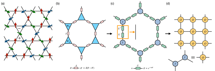
Figure 5: Tensor network representation of the fully frustrated XY model on the kagome lattice. (a) One of the ground state configurations. The positive and minus signs denote the chiralities on the triangular plaquettes. (b) The tensor network with continuous indices. The $W_{\Delta}$ and $W_{\nabla}$ tensors represent the Boltzmann weight on up and down-type triangles. The $\delta$ matrix represents the Dirac delta function. (c) The construction of tensor network with discrete indices by making Fourier transformation on each triangle plaquette and integrating out $\{\theta\}$ variables. (d) The tensor network representations composed of local uniform tensor $O$, where the $O$ tensor is built by combining two neighboring $I$ tensors

To describe the Josephson junction array under a uniform external magnetic fieldTeitel and Jayaprakash (1983); Park and Huse (2001), the frustrated XY model on a kagome lattice in Fig. 5 (a) is defined by the Hamiltonian

$$H=-J\sum_{\langle i,j\rangle}\cos(\theta_{i}-\theta_{j}-A_{ij})$$ (25)

where $J>0$ is the coupling strength, $i$ and $j$ are the lattice sites, and the summation is over all pairs of the nearest neighbors. The frustration in this model is induced by the gauge field defined on the lattice bond satisfying $A_{ij}=-A_{ji}$. The case of full frustration corresponds to one-half flux quantum per plaquette,

$$f=\frac{1}{2\pi}\sum_{\langle i,j\rangle\in\Delta}A_{ij}=\frac{1}{2},$$ (26)

where the sum is taken around the perimeter of a plaquette. We can choose the fixed gauge condition of $A_{ij}=\pm\pi$ on each bond of the triangular plaquettes, and the model is transformed into an AF XY model on the kagome lattice

$$H=J\sum_{i,j}\cos(\theta_{i}-\theta_{j}).$$ (27)

The ground state of this model can be obtained by simultaneously minimizing the energy on each elementary triangle. As shown in Fig. 5(a), the phase difference between each pair of neighboring spins should be $\pm 2\pi/3$. which gives rise to the emergent degrees of freedom of chiralities $\tau=\pm 1$, corresponding to the anti-clockwise and clockwise rotation of the spins around the plaquette. The ground state of the AF XY model on a kagome lattice has a massive accidental degeneracy described by the fluctuations of the chiralities.

To capture the emergent degrees of freedom induced by frustrations in the construction of the tensor network, we divide the Hamiltonian into local terms on each triangle:

$$H=\sum_{p}H_{p},$$ (28)

where $H_{p}$ includes all the interactions within an elementary triangle

$$H_{p}=J\sum_{\langle i,j\rangle\in p}\cos(\theta_{i}-\theta_{j}).$$ (29)

The partition function can now be written as

$$Z=\prod_{i}\int\frac{d\theta_{i}}{2\pi}\prod_{p}W_{p},$$ (30)

where $W_{p}=\mathrm{e}^{-\beta H_{p}}$ is a three-legged tensor with continuous $U(1)$ indices and the constraint of sharing the same spin at the corners is realized by the Dirac delta function $\delta(\theta_{i}-\theta_{i}^{\prime})$, as shown in Fig. 5 (b).

To transform the local tensors onto a discrete basis, we employ the duality transformation to the whole upward triangles

$$I_{n_{1},n_{2},n_{3}}=\prod_{i=1}^{3}\int\frac{d\theta_{i}}{2\pi}W_{\Delta}(\theta_{1},\theta_{2},\theta_{3})U_{n_{1}}(\theta_{1})U_{n_{2}}(\theta_{2})U_{n_{3}}(\theta_{3}),$$

and the downward triangles

$$I^{\prime}_{n_{1},n_{2},n_{3}}=\prod_{i=1}^{3}\int\frac{d\theta_{i}}{2\pi}W_{\nabla}(\theta_{1},\theta_{2},\theta_{3})U_{n_{1}}^{\dagger}(\theta_{1})U_{n_{2}}^{\dagger}(\theta_{2})U_{n_{3}}^{\dagger}(\theta_{3}),$$

where

$$U_{n}(\theta)=\mathrm{e}^{-in\theta}$$ (31)

are the basis of the Fourier transformation. Since $W_{p}$ is unchanged under the spin reflection of $\theta\to-\theta$, we have $I_{n_{1},n_{2},n_{3}}=I^{\prime}_{n_{1},n_{2},n_{3}}$ as displayed in Fig. 5 (c). Meanwhile, the duality transformation on the Dirac delta function gives the Kronecker delta function

$$\int\frac{d\theta}{2\pi}U_{n_{1}}^{\dagger}(\theta)U_{n_{2}}(\theta)=\delta_{n_{1},n_{2}}.$$ (32)

Finally, the translation-invariant local tensor $O$ is achieved by combining a pair of $I$ tensors and we arrive at the the uniform tensor network representation of the partition function

$$Z=\mathrm{tTr}\prod_{i}O_{s_{1},s_{2}}^{s_{3},s_{4}}(i)$$ (33)

as shown in Fig. 5 (d). In fact, the same tensor network has been also obtained in a less straightforward way with the help of the infinite summation, where the interactions between emergent variables can be seen clearlySong and Zhang (2023). A direct comparison to the problematic standard construction in Ref. Song and Zhang (2023) demonstrates the importance of encoding the emergent degree of freedom in the local tensors: besides the proper Hamiltonian tessellation, the duality transformation is also necessary to capture the essential physics of the chiralities.

In the framework of tensor networks, the entanglement entropy of the fixed-point MPS for the 1D quantum correspondence exhibits singularity at the critical temperatures, offering a sharp criterion to determine possible phase transitions in the thermodynamic limit. As shown in Fig. 6, by employing the tensor network method outlined in the Appendix, the entanglement entropy $S_{E}$ develops only one sharp singularity at the critical temperature $T_{c}\simeq 0.075J$, indicating that a single BKT phase transition takes place at a rather low temperature. The peak positions are almost unchanged with different MPS bond dimensions ranging from $D=60$ to $120$. Thus, the transition temperature is determined with high precision, which is in good agreement with theoretical predictions for the unbinding temperature of $1/3$ vortex pairsCherepanov et al. (2001); Korshunov (2002); Song and Zhang (2023). The low-temperature phase of the model can be interpreted as the presence of charge-6e superconductivity (SC) in the absence of charge-2e SCSong and Zhang (2023).

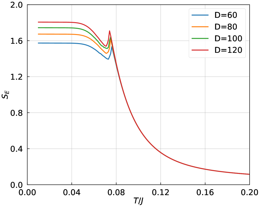
Figure 6: The entanglement entropy as a function of temperature under different MPS bond dimensions for the AF XY spin model on the kagome lattice.

III.3 Fully Frustrated XY spin model on a square lattice

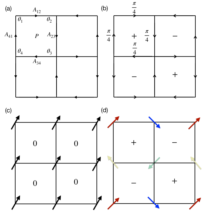
Figure 7: (a) The fully frustrated XY model on a square lattice. The arrows on the links correspond to the gauge field ${A_{ij}}$ with the value of $\pm\frac{\pi}{4}$. The sign of $A_{ij}$ is denoted by the direction of the arrow. (b) The ground state of the FFXY model on a square lattice with a checkboard pattern of chirality. (c) The ground state of the modified XY model for $\frac{\mu}{J}<\frac{1}{8}$. (d) The ground state of the modified XY model for $\frac{\mu}{J}>\frac{1}{8}$. The $0,\pm$ signs correspond to the topological charges located on the centers of the plaquettes.

The fully frustrated XY (FFXY) spin model on a 2D square lattice can be defined with gauge fields on the lattice bonds

$$H=-J\sum_{\langle i,j\rangle}\cos(\theta_{i}-\theta_{j}-A_{ij}),$$ (34)

where the full frustration corresponds to the uniform gauge field of $A_{ij}=\pi/4$ on each bond of the square plaquettes. As displayed in Fig. 7 (b), the minimum of the Hamiltonian is obtained when all gauge-invariant phase differences between nearest-neighbor spins $\phi_{i,j}=\theta_{i}-\theta_{j}-A_{ij}$ equal to $\pm\pi/4$. The ground state can be characterized by a checkerboard pattern of chiralities $\tau=\pm 1$ defined by $\sum_{\square}\phi_{i,j}=\tau\pi$. Another degenerate state can be obtained by switching the positive and negative chiralities. Therefore, in addition to the $U(1)$ symmetry, the chiralities give rise to an emergent $Z_{2}$ degeneracy of the ground state of the FFXY model on a square lattice Villain (1977a, b); Song and Zhang (2022).

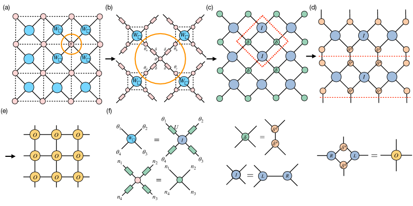
Figure 8: Tensor network representation of the FFXY model on a square lattice. (a) The tensor network with continuous indices, where the $W$ tensors account for the Boltzmann weight on each square and the pink dot tensor accounts for the integration of the shared $\theta$ variables among four plaquettes. The black dotted line denotes the original square lattice. (b) The auxiliary spin $\theta^{\prime}$ connecting the copied spins of four nearby plaquettes, the $\delta$ matrices represent the Dirac delta functions. (c) The tensor network with discrete indices obtained from Fourier transformations on the $W$ tensors and the integrations on the $\theta$ variables. (d) The row-to-row transfer matrix built by splitting the $\delta$ tensors vertically. (e) The uniform tensor network representation composed of local tensor $O$. (f) The details of the operations on the local tensors in the construction of the tensor network.

To obtain the tensor network representation of the partition function, we first divide the global Hamiltonian into a tessellation of local Hamiltonian on each square where the emergent variables live

$$H=\sum_{\square}H_{\square},$$ (35)

and the local cluster of interactions is given by

$$H_{\square}=-\frac{J}{2}\sum_{\langle i,j\rangle\in{\square}}\cos(\theta_{i}-\theta_{j}-A_{ij}).$$ (36)

Then the tensor network can be expressed as a product of local Boltzmann weights on each plaquette as shown in Fig. 8 (a)

$$Z=\prod_{i}\int\frac{d\theta_{i}}{2\pi}\prod_{\square}W_{\square}$$ (37)

where $W_{p}(\theta_{1},\theta_{2},\theta_{3},\theta_{4})=\mathrm{e}^{-\beta H_{\square}}$ is a four-legged tensor with a continuous $U(1)$ indices.

Different from the corner-shared case of the kagome lattice, particular attention should be paid to the split of the shared spins among four square plaquettes. To avoid the formation of loops of the Dirac delta functions among four $W$ tensors

$$\delta(\theta_{a}-\theta_{b})\delta(\theta_{b}-\theta_{c})\delta(\theta_{c}-\theta_{d})\delta(\theta_{d}-\theta_{a})$$

with $\theta_{a}$, $\theta_{b}$, $\theta_{c}$ and $\theta_{d}$ representing the four replicas of the shared spin, we put an auxiliary spin $\theta_{i}^{\prime}$ connecting to the shared spins

$$\delta(\theta_{a}-\theta^{\prime})\delta(\theta_{b}-\theta^{\prime})\delta(\theta_{c}-\theta^{\prime})\delta(\theta_{d}-\theta^{\prime})$$

in a star shape as shown in Fig. 8 (b). Then we transform the local tensor $W_{p}$ to the discrete basis

$$I_{n_{1},n_{2},n_{3},n_{4}} = \prod_{i=1}^{4}\int\frac{d\theta_{i}}{2\pi}W_{\Delta}(\theta_{1},\theta_{2},\theta_{3},\theta_{4})$$ (38)

$$\cdot U_{n_{1}}(\theta_{1})U_{n_{2}}(\theta_{2})U_{n_{3}}(\theta_{3})U_{n_{4}}(\theta_{3}),$$

where $U_{n}(\theta)$ are the Fourier basis defined in (31).

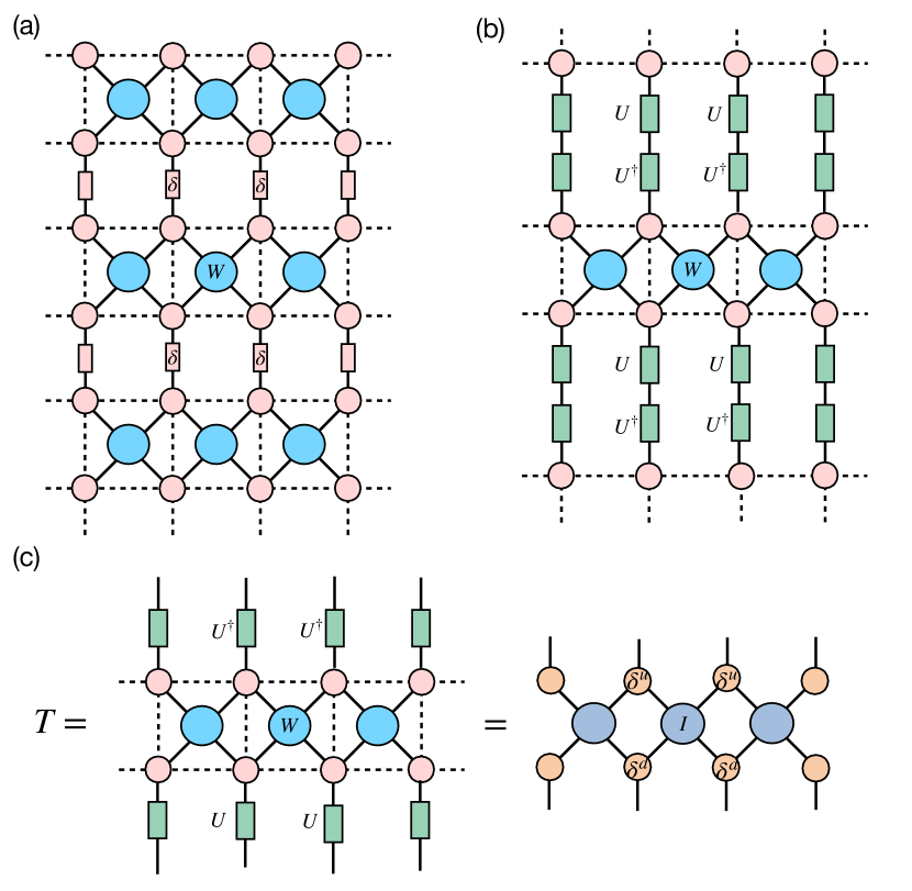
Figure 9: (a) Tensor network representation of the partition function with the split of $U(1)$ phase variables vertically. The $\delta$ matrices represent the Dirac delta functions. (b) The decomposition of the Dirac delta function into $U$ matrix and $U^{\dagger}$ matrices. (c) The row-to-row transfer matrix on the continuous basis and the discrete basis, respectively.

As shown in Fig. 8 (f), the constraint of the star-shaped Dirac delta functions (III.3) can be reduced to a four-legged Kronecker delta tensor via

$$\delta_{n_{1}+n_{2}+n_{3}+n_{4},0}=\int\frac{d\theta^{\prime}}{2\pi}U_{n_{1}}(\theta^{\prime})U_{n_{2}}(\theta^{\prime})U_{n_{3}}(\theta^{\prime})U_{n_{4}}(\theta^{\prime})$$

characterizing the conservation law of $U(1)$ charges. As a result, we get the tensor network representation composed of local tensors of discrete indices as displayed in Fig. 8 (c).

Furthermore, the $\delta$ tensors are split vertically as shown in Fig. 8 (d),

$$\delta_{n_{1}+n_{2}+n_{3}+n_{4},0}=\sum_{n_{5}}\delta_{n_{1}+n_{2}-n_{5},0}^{u}\delta_{n_{3}+n_{4}+n_{5},0}^{d}$$ (39)

and the $I$ tensors are decomposed horizontally by SVD

$$I_{n_{1},n_{2},n_{3},n_{4}}=\sum_{n_{5}}L_{n_{1},n_{2},n_{5}}R_{n_{5},n_{3},n_{4}}$$ (40)

as displayed in Fig. 8 (f). Finally, the regular local tensor $O$ in the uniform tensor network of Fig. 8 (e) is obtained by grouping the relevant component tensors.

One might rotate the network in Fig. 8 (c) by $45$ degrees and group the local tensors in the red dotted line to directly make up a four-legged translation-invariant local tensor. However, the standard contraction algorithms fail to converge under this construction because the linear transfer matrix is non-Hermitian. Another key insight is that such a construction does not take into account the checkerboard-like ground state configurations, where only two chiralities are included in the transitional unit.

Actually, although the procedure of the construction is different, the tensor network in Fig. 8 turns out to share the same transfer matrix as the one obtained in the Ref. Song and Zhang (2022). To prove it, we split the $U(1)$ spins in the vertical direction using the relation

$$\int d\theta_{i}f(\theta_{i})=\iint d\theta_{i}d\theta_{i}^{\prime}\delta(\theta_{i}-\theta_{i}^{\prime})f(\theta_{i}^{\prime}),$$ (41)

where the spin $\theta_{i}^{\prime}$ is a copy of spin $\theta_{i}$ connected by the Dirac delta function as shown in Fig. 9 (a). The delta tensor on a link can be further decomposed by the Fourier basis

$$\delta(\theta-\theta^{\prime})=\frac{1}{2\pi}\sum_{n}U_{n}^{\dagger}(\theta^{\prime})U_{n}(\theta),$$ (42)

as displayed in Fig. 9 (b). Now we can define the row to row transfer matrix as three stripes of $U$, $W$ and $U^{\dagger}$ tensors as shown in Fig. 9 (c). It is easy to see that the transfer matrix is Hermitian just like the one constructed in Ref.Song and Zhang (2022) since the $W$ tensors are real and symmetric. Using the Fourier transformation again, we get the same $I$ and $\delta$ tensors in Fig. 9 (c) as those displayed in Fig. 8 (d).

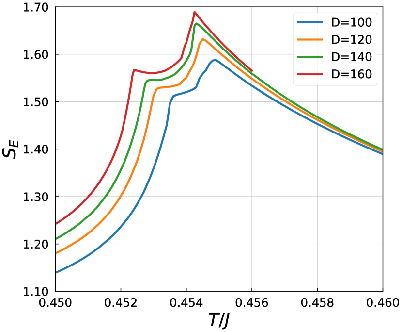
Figure 10: The entanglement entropy for the FFXY model on the square lattice develops two singularities indicating the existence of two phase transitions with the increasing of MPS bond dimensions.

Once the proper tensor network representation is obtained, the numerical calculations can be efficiently performed as illustrated in the Appendix. As shown in Fig. 10, the entanglement entropy $S_{E}$ develops two sharp singularities at two critical temperatures $T_{c1}$ and $T_{c2}$, which strongly indicates the existence of two phase transitions at two different temperatures. As the singularity positions vary with the MPS bond dimension $D$, the critical temperatures $T_{c1}$ and $T_{c2}$ can be determined precisely by extrapolating the bond dimension $D$ to infinite. Moreover, we find that the critical temperatures $T_{c1}$ and $T_{c2}$ exhibit different scaling behaviors in the linear extrapolation, implying that the two phase transitions belong to different kinds of universality classes. The lower transition temperature $T_{c1}$ varies linearly on the inverse square of the logarithm of the bond dimension, while the higher transition temperature $T_{c2}$ has a linear variance with the inverse bond dimension. The different scaling behavior agrees well with the different critical behavior of the BKT and 2D Ising universality classesSong and Zhang (2022).

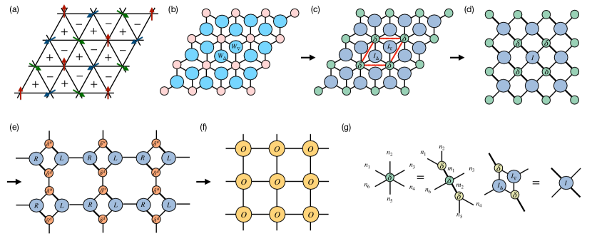
Figure 11: The tensor network representation of the FFXY model on a triangular lattice. (a) One of the ground state spin configurations. The chiralities denoted by plus and minus signs on the centers of the triangular plaquettes form an AF pattern. (b) The tensor network with continuous indices. (c) The tensor network is transformed onto a discrete basis through the Fourier transformation. A parallelogram unit cell is circled in the red line. (d) The $I$ tensors is constructed by grouping a pair of $I_{\nabla}$ and $I_{\Delta}$ tensors. (e) The vertical split of the $\delta$ tensors into $\delta^{d}$ and $\delta^{u}$ and the horizontal split of the $I$ tensors into $L$ and $R$. (f) The tensor network representation composed of uniform local $O$ tensors. (g) Details of the transformations of local tensors.

III.4 AF XY spin model on a triangular lattice

The frustrated XY spin model on a triangular lattice under a fixed gauge condition of $A_{ij}=\pi$ on each triangular plaquette can be transformed into an AF XY spin model. As shown in Fig. 11 (a), the angle between each pair of the nearest-neighbor spins should be $\pm 2\pi/3$ to achieve the minimum of the ground state energy. Like the FFXY model on the square lattice, the elementary triangular plaquettes can be characterized by alternating chiralities of $\tau=\pm 1$. The translation-invariant unit of the spin configuration forms a $3\times 3$ cluster larger than the original lattice.

The tensor network can be constructed in the same way as the FFXY spin model on the square lattice. First, we decompose the Hamiltonian into local terms on each triangle

$$H=\sum_{p}H_{p},\hskip 14.22636ptH_{p}=\frac{J}{2}\sum_{\langle i,j\rangle\in p}\cos(\theta_{i}-\theta_{j}).$$ (43)

The partition function can be expressed as a product of local Boltzmann weights

$$Z=\prod_{i}\int\frac{d\theta_{i}}{2\pi}\prod_{p}W_{p},$$ (44)

where $W_{p}=\mathrm{e}^{-\beta H_{p}}$ defined on the centers of the triangles are three-legged tensors sharing the same $U(1)$ spin at the joint corners as shown in Fig. 11 (b).

Then the $W$ tensors and the Dirac delta functions are transformed onto a discrete basis by the Fourier transformations, as displayed in Fig. 11 (c). To achieve a transition-invariant unit, we take a parallelogram cell circled by the red line and reorganize the local tensors within it. As shown in Fig. 11 (g), the six-legged delta tensor is decomposed into three smaller delta tensors

$$\delta_{n_{1}+n_{2}+n_{3}+n_{4}+n_{5}+n_{6},0}$$

$$= \sum_{m_{1},m_{2}}\delta_{n_{1}+n_{2},m_{1}}\delta_{m_{1}+n_{3}+m_{2}+n_{6},0}\delta_{n_{4}+n_{5},m_{2}},$$

where the bond dimension of the $m$-indexed leg is bigger than the $n$-indexed leg denoted by a thicker line. At the same time, a pair of $I_{\Delta}$ and $I_{\nabla}$ tensors are grouped together into a four-legged $I$ tensor

$$I_{n_{1},m_{2},n_{3},m_{4}} = \sum_{n_{2},n_{4},n_{5},n_{6}}\delta_{n_{2}+n_{4},m_{2}}$$

$$(I_{\Delta})_{n_{1},n_{2},n_{5}}\delta_{n_{5}+n_{6},m_{4}}(I_{\nabla})_{n_{3},n_{4},n_{6}},$$

and the tensor network is transformed to a relatively structured form in Fig. 11 (d). Following the same procedure of a vertical split of the $\delta$ tensors and a horizontal split of the $I$ tensors, we obtain the uniform tensor network in Fig. 11 (f).

Note that the Fourier transformation must be performed on each triangular plaquette first to ensure the emergence of the dual variables. Otherwise, if we directly choose a parallelogram including a pair of neighboring triangles and then build the tensor network based on the local Boltzmann weight of

$$W_{\hbox to0.0pt{\rotatebox{-30.0}{\rule[0.1507pt]{0.4pt}{5.39003pt}}\hss}\kern 0.27995pt\hbox to0.0pt{\kern 2.52pt\raisebox{4.54665pt}{\rule{4.20004pt}{0.4pt}}\hss}\rule{4.20004pt}{0.4pt}\kern-0.27995pt\rotatebox{-30.0}{\rule[0.1507pt]{0.4pt}{5.39003pt}}}(\theta_{1},\theta_{2},\theta_{3},\theta_{4})$$

$$=\exp\Big{\{}-\frac{\beta J}{2}[\cos(\theta_{1}-\theta_{2})+\cos(\theta_{2}-\theta_{3})$$

$$+\cos(\theta_{3}-\theta_{4})+\cos(\theta_{4}-\theta_{1})+2\cos(\theta_{1}-\theta_{3})]\Big{\}},$$

the infinite contraction of the tensor network will not give the right results. The reason is that the construction of local tensors with a finite bond cut-off can be regarded as a coarse-grained procedure that should be performed exactly on the clusters of spin corresponding to the emergent degrees of freedom.

As shown in Fig. 12, the entanglement entropy $S_{E}$ also develops two sharp singularities at two critical temperatures $T_{c1}$ and $T_{c2}$, and the critical temperatures have the same scaling behavior as the FFXY model on the square lattice. From the linear extrapolation, the critical temperatures are estimated to be $T_{c1}\simeq 0.5060J$ and $T_{c2}\simeq 0.5116J$. The critical temperature $T_{c1}$ agrees well with previous Mont Carlo results Obuchi and Kawamura (2012) obtained by BKT fitting and $T_{c2}$ is slightly lower than a recent estimation Obuchi and Kawamura (2012); Lv et al. (2013) of $T_{c2}\simeq 0.512J$.

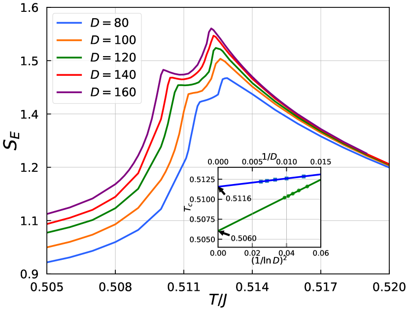
Figure 12: For the AF XY model on the triangular lattice, the entanglement entropy as a function of temperature develops two peaks when the MPS bond dimension $D$ is increased. Inset: The singularity temperatures $T_{c1}$ and $T_{c2}$ of the entanglement entropy fitted for MPS bond dimensions from $D=80$ to $160$.

The properties of the two distinct phase transitions can be further elucidated through the thermodynamic quantities. The results of the specific heat are presented in Fig. 13 (a). Around the critical temperature $T_{c1}$, the specific heat exhibits a small bump, indicating a higher-order continuous phase transition. By comparison, the specific heat displays a sharp divergence at $T_{c2}$, implying a second-order phase transition. For the high-temperature side $T>T_{c2}$, the specific heat can be fitted well by the logarithmic behavior of a second-order Ising transition. The specific heat between $T_{c1}$ and $T_{c2}$ does not fit well with the logarithmic form due to the close proximity of the two transitions. The breaking of $Z_{2}$ symmetry at $T_{c2}$ can be demonstrated by the expectation values of the chiralities. As shown in Fig. 13 (b), below the critical temperature $T_{c2}$, the chiral order parameter

$$m=\frac{1}{N}\sum_{p}(-1)^{x+y}\tau_{p}$$ (45)

associated with the chiral degrees of freedom establishes a non-zero value, corresponding to the checkerboard pattern of chirality on upward and downward triangles. When approaching the critical temperature $T_{c2}$ from the low-temperature side, the order parameter vanishes continuously as $m\sim t^{\beta}$ with $t=1-T/T_{c2}$. The critical exponent $\beta\simeq 0.1238$ is in good agreement with the critical exponent $\beta=1/8$ for the 2D Ising universality class.

The nature of the phase transition at $T_{c1}$ can be revealed in the change of the behavior of the spin-spin correlation functions defined as

$$G(r)=\langle\cos(\theta_{i}-\theta_{i+r})\rangle.$$ (46)

A comparison of correlation functions below and above $T_{c1}$ is displayed in Fig. 13(c) and (d). Below $T_{c1}$, the spin-spin correlation function exhibits a power-law decay, implying a close binding between vortices and anti-vortices. In contrast, for $T>T_{c1}$ the correlation function displays an exponential decay, indicating the destruction of phase coherence between vortices due to the unbinding of vortex pairs. Thus, the phase transition at $T_{c1}$ belongs to the universality class of the BKT transition.

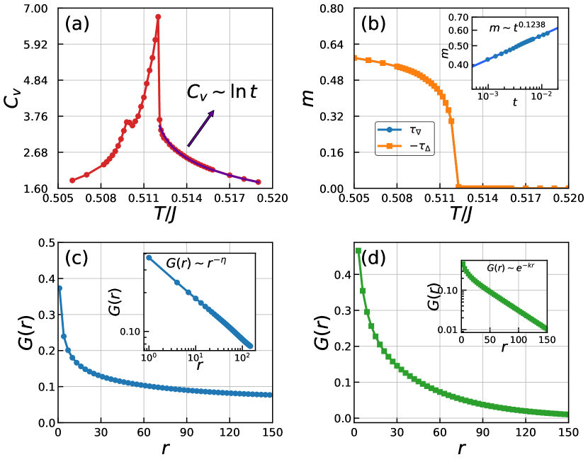
Figure 13: (a) The specific heat shows a small bump around $T_{c1}$ but a logarithmic divergence at $T_{c2}$. (b) The symmetry breaking of chirality at $T_{c2}$. The inset is the fitting of the Ising critical exponent. (c) The spin-spin correlation function shows a power-law decay below $T_{c1}$ (d) The spin-spin correlation function shows an exponential decay above $T_{c1}$.

III.5 Modified XY model on a square lattice

The unified tensor network methods can be employed in the study of frustrated spin models with more complex interactions. One such model is the modified XY model defined on a 2D square lattice Maccari et al. (2020, 2023)

$$H=-J\sum_{\langle i,j\rangle}\cos(\theta_{i}-\theta_{j})-\mu\sum_{p}\tau_{p}^{2},$$ (47)

where the first term is the original XY model of ferromagnetic coupling $J>0$, and the second term tunes the vortex fugacity through the chemical potential $\mu$. The spin current circulating around each single square plaquette is defined as

$$\tau_{p}=\sum_{\langle i,j\rangle\in p}\sin(\theta_{i}-\theta_{j}).$$

It is well-known that the original XY spin model can be mapped into an interacting Coulomb gas with a vortex-core energy fixed in the low-density limit Kosterlitz and Thouless (1973); Kosterlitz (1974). And the underlying physics at large vortex density is of general interest both theoretically and experimentally. In the area of theoretical investigations, the possible extension of BKT theory under a large vortex fugacity was discussed, where non-BKT behavior and the occurrence of first-order transition were proposed Minnhagen (1985a, b, 1987); Zhang et al. (1993). Actually a generalization of 2D XY spin model with a ”crossed-product” operator acting on the plaquettes had been introduced to adjust the core energy of the vortices Swendsen (1982). Subsequently, the numerical explorations of a Coulomb gas model on the square and triangular lattices as well as in the continuous limit showed a rich phase diagram with novel critical behaviors of an ordered-charge lattice Lee and Teitel (1990, 1991); Lidmar and Wallin (1997). Moreover, the similar physics has been investigated in 3D XY spin models, where a term acting on the plaquette was introduced to regulate the energy of vortex strings Kohring et al. (1986); Shenoy (1990).

The experiments in superconducting thin films revealed a significant deviation of the vortex-core energy from the predictions in the original XY model Kamlapure et al. (2010). It was found that an accurate consideration of the vortex-core energy is of great importance for the experimental identification of the BKT transition Mondal et al. (2011). Apart from the widely known superfluid phase and normal phase, the measurement of the third sound mode in ⁴He thin films suggested the existence of a new phase Chen et al. (1992). To provide a theoretical explanation for this phenomenon, researchers have proposed a fascinating concept involving the formation of a lattice composed of vortices and anti-vortices, with a remarkably low vortex core energy Zhang (1993); Gabay and Kapitulnik (1993). The existence of vortex-antivortex lattice has also been proposed in other systems such as ultra-cold atoms Botelho and Sá de Melo (2006) and polariton fluids Hivet et al. (2014).

To understand the role of the modified interaction term $\tau_{p}$, we can make a simple analysis of the ground state. The ground state structure can be determined by the ratio of $\mu/J$ tuning the spin currents in the system which effectively modulates the vortex fugacity. As illustrated in Fig. 7(c)-(d), when $\mu/J<1/8$, the ground state is identical to that at $\mu=0$, corresponding to the ground state of the original XY model where all spins align parallel to each other. As we further increase the chemical potential to $\mu/J>1/8$, the ground state is characterized by maximizing $\tau_{p}$ on each plaquette, resulting in a phase difference of $\phi_{12}=\phi_{23}=\phi_{34}=\phi_{41}=\pm\pi/2$. This ground state has the same ground state degeneracy as the FFXY spin model on a square lattice. From the perspective of vorticity, the ground state at $\mu/J<1/8$ has zero vorticity at each plaquette termed as the vortex vacuum state, whereas the ground state at $\mu/J>1/8$ has a checkerboard pattern of vorticity equal to $\pm 1$ called the vortex-antivortex crystal. Hence, the zero-temperature ground state structure of the modified XY spin model is analogous to the 2D dense coulomb gas on the square lattice Lee and Teitel (1990).

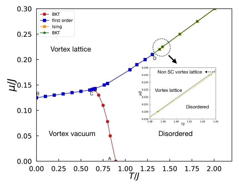
Figure 14: The global phase diagram of the modified XY spin model. The BKT transition point A of the original XY spin model is determined as $(0.893,0)$. The exact solvable point B between the vortex vacuum phase and vortex lattice phase at zero temperature is given by $(0.0,0.125)$. As the temperature increases, depending on the chemical potential, the vortex lattice can melt through three possible way. Below the point C at $(0.64,0.142)$, the vortex lattice experiences a first-order transition into the vortex vacuum phase and then undergoes a BKT transition into the disordered phase, while the CD line is the first-order transition. The point D is a tricritical point determined as $\mu/J\simeq 0.21$. Above this point D, the first order transition line is separated into two extremely close transition lines, belonging to the BKT transition and Ising transition, respectively. Inset shows the enlarged results around the point $D$.

The square term $\tau_{p}^{2}$ gives rise to multiple types of interaction including the nearest-neighbor interactions, next-nearest-neighbor interactions, and four-body interactions. Although it seems difficult to treat the four-body interactions, there is still a well-defined vorticity on each plaquette from the viewpoint of emergent degrees of freedom. Therefore we can choose each square plaquette as an elementary cluster and replace the $H_{p}$ and $W_{p}$ by

$$H_{p}=-\frac{J}{2}\sum_{\langle i,j\rangle\in p}\cos(\theta_{i}-\theta_{j})-\mu\tau_{p}^{2},\quad W_{p}=\mathrm{e}^{-\beta H_{p}}.$$ (48)

Then the tensor network of the partition function can be constructed following the procedure outlined in Fig. 8. The singular behavior of the entanglement entropy corresponding to the 1D transfer operator offers a sharp criterion to determine all possible phase transitions in the thermodynamic limit and the complete phase diagram is thus determined as presented in Fig. 14.

In the upper plane of the phase diagram, the entanglement entropy along the chemical potential $\mu=0.3J$ is displayed in Fig. 15 (a). There exist two distinct peaks, corresponding to the BKT and Ising transition, respectively. These two phase transitions are extremely close to each other as shown by the zoomed inset in Fig. 14. Upon further reducing the chemical potential to $\mu\simeq 0.20J$, two separated peaks merge into a single peak, as displayed in Fig. 15 (b). The merging point is denoted as the point $D$ in the global phase diagram. The low-temperature phase with large $\mu$ is called the vortex-lattice phase due to the checkerboard pattern of vortices and anti-vortices coexisting with the SC order. The chiral LRO is demonstrated by the finite expectation value of chiralities (45) as shown in Fig. 16 (b) and Fig. 17 (b). The SC order is characterized by the quasi-LRO of $U(1)$ spins, where the spin-spin correlation function (46) displays a power-law decay as displayed in Fig. 16 (d). The melting of the vortex lattice undergoes two steps into the disordered phase with an intermediate non-SC vortex-lattice phase. In the non-SC vortex-lattice phase, the chiral LRO survives but the phase coherence between vortices is destroyed. Such a two-step procedure has been extensively investigated in the FFXY models Villain (1977a, b); Song and Zhang (2022).

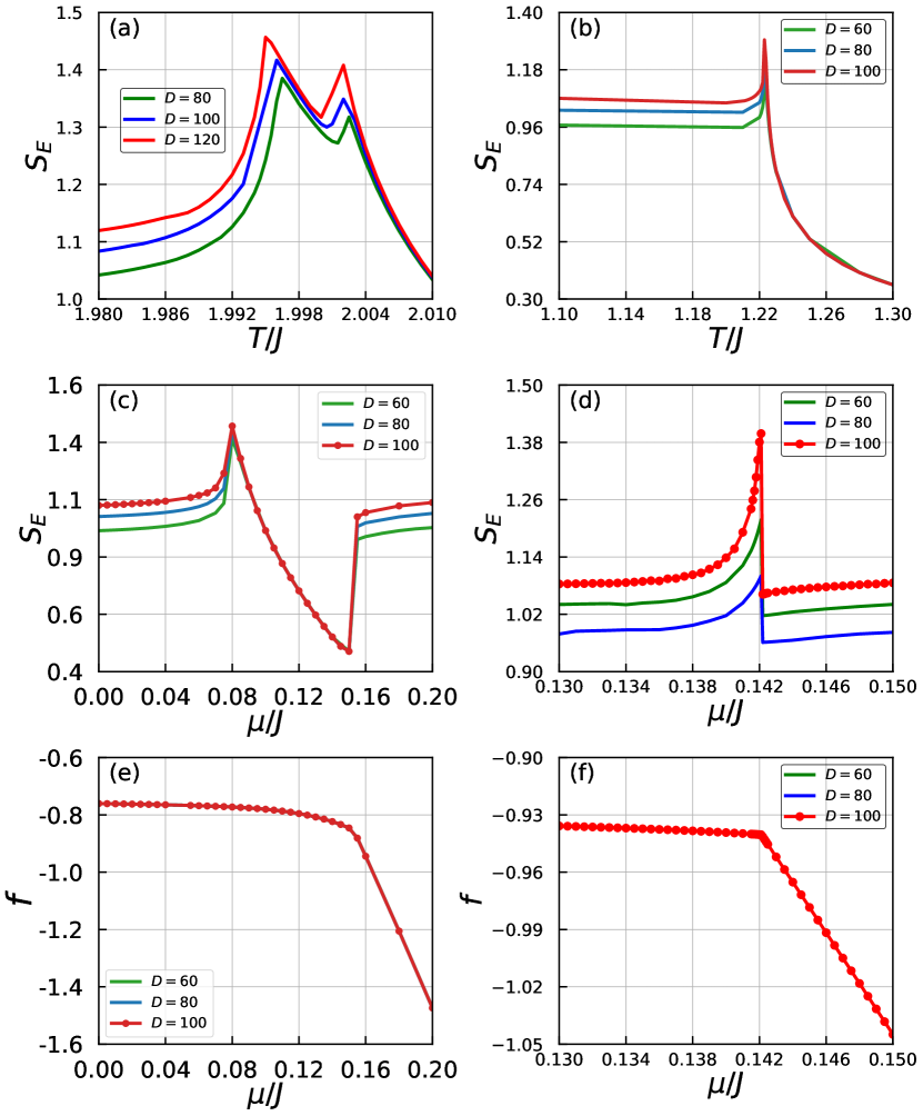
Figure 15: (a) The entanglement entropy as a function of temperature along $\mu=0.3J$. (b) The entanglement entropy as a function of temperature along $\mu\simeq 0.20J$. (c) The entanglement entropy as a function of chemical potential along $T=0.8J$. (d) The entanglement entropy as a function of chemical potential along $T=0.64J$. (e) The free energy density as a function of chemical potential along $T=0.8J$. (f) The free energy density as a function of chemical potential along $T=0.64J$.

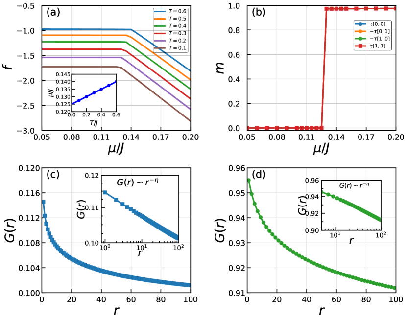
Figure 16: (a) The free energy density as a function of chemical potential at different temperatures. Inset: linear extrapolation of critical chemical potential as a function of temperature. (b) The checkboard-like chirality pattern along $T=0.1J$. (c) The spin-spin correlation function shows an exponential decay at $T\simeq 0.1J$ and $\mu\simeq 0.1J$ in the vortex-vacuum phase. (d) The spin-spin correlation function shows a power-law decay at $T\simeq 0.1J$ and $\mu\simeq 0.15J$ in the vortex-lattice phase.

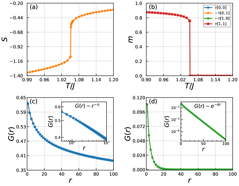
Figure 17: (a) The thermal entropy density as a function of temperature along $\mu=0.18J$. (b) The chirality on $2\times 2$ sublattice as a function of temperature along $\mu=0.18J$. (c) The spin-spin correlation function at $T\simeq 1.05J,$ and $\mu\simeq 0.18J$ in vortex lattice phase shows a power-law decay. (d) The spin-spin correlation function at $T\simeq 1.06J$ and $\mu\simeq 0.18J$ in disorderd phase displays an exponential decay.

Below the point $D$, the phase boundaries are determined by a combined analysis of the entanglement entropy and free energy. We find that the fixed-point equations have two different solutions across the critical point depending on the initial states we start from. The proper solution is chosen with a lower free energy density. As shown in Fig. 15 (c), along the line $T=0.8J$, the entanglement entropy exhibits a peak at $\mu\simeq 0.080J$ corresponding to the BKT transition and a discontinuous jump at $\mu\simeq 0.153J$ associated to a first-order phase transition. The free energy density of Fig. 15 (e) displays an inflection point of a first-order transition at $\mu\simeq 0.153J$, demonstrating that the entanglement entropy can serve as a powerful criterion for the determination of the first-order phase transition. Besides, we find that the position of the first-order transition is nearly unchanged with increasing bond dimensions, in good agreement with the behavior of the entanglement entropy. As the temperature decreases, the BKT transition line $CA$ and the first-order transition line $CD$ become closer and finally merge into a single first-order transition line $CB$ at the tricritical point $C$ with $T\simeq 0.640J$ and $\mu\simeq 0.142J$. As shown in Fig. 15 (d), along the line $T=0.64J$, the entanglement entropy shows a discontinuous jump just above the peak position of $\mu\simeq 0.142J$. The corresponding free energy density is displayed in Fig. 15 (f) with an evident cusp point.

Across the transition line $CD$, the vortex lattice melts directly into the disordered phase via a first-order transition, where the chiral LRO and spin quasi-LRO break down simultaneously. As is shown in Fig. 17 (a) and (b), both the thermal entropy density $S$ and the chiral order parameter $m$ develop a discontinuous jump at the transition point of $\mu\simeq 0.18$ and $T\simeq 1.052$. A comparison between the spin-spin correlation functions across the line $CD$ is displayed in Fig. 17 (c) and (d). For a given temperature of $T=1.05J$ in the vortex-lattice phase, the correlation function $G(r)$ displays a power-law behavior. But in the disordered phase with $T=1.06J$, the correlation function behaves in an exponential way. We should point out that the existence of a novel continuous transition arising from the merging of BKT and Ising transitions Granato and Kosterlitz (1986); Granato (1987); Lee et al. (1991); Li and Cieplak (1994); Nightingale et al. (1995) is not found here.

At low temperatures, the phase boundary $CB$ belongs to a first-order transition between the vortex-lattice phase and the vortex-vacuum phase. As shown in Fig. 16(b), when going down along $T=0.1J$ line, the chiral order parameter $m$ exhibits a discontinuous jump to zero at $\mu\simeq 0.128J$. Since the vortex fugacity is greatly suppressed by decreasing the chemical potential $\mu$, the vortex density drops dramatically, driving the system into the vortex-vacuum phase. Note that the “vortex vacuum” just means that there is no excitation of free vortices but the charge-neutral vortex-antivortex pairs can still be excited. The excitation of vortex-antivortex pairs destroys the LRO of the $U(1)$ spins and gives rise to the well-known BKT quasi-LRO state. As can be seen in Fig. 16 (c)-(d), the spin-spin correlation function displays a power-law decay in both the vortex-lattice and vortex-vacuum phases. When the temperature further decreases, the first-order transition line $CB$ behaves in a linear way. Such a linear behavior is displayed in Fig. 16 (a), where the extrapolation to the zero temperature gives $\mu=0.125J$ in the inset. The terminal point $B$ is determined at $T=0$ and $\mu=0.125J$, consistent with our previous analysis of the ground state.

Finally, the transition line $CA$ separating the vortex-vacuum and disordered phase is the conventional BKT transition, driven by the dissociation of vortex-antivortex pairs. The inverse process, when the system is cooling from a disordered phase, pairs of vortex and anti-vortex appear and further condensed into a square vortex lattice is analogous to the theoretical proposal in ultracold Fermi gases Botelho and Sá de Melo (2006). The rich phase diagram of the modified XY model provides important insights into the formation of the vortex lattice and the complex melting process. By tuning the vortex chemical potential, the unconventional phase transitions in SC lattice are investigated thoroughly in the orientational $U(1)$ phase variables. A more comprehensive study should take into account the positional order since the vortex lattice may also melt via the Kosterlitz-Thouless-Halperin-Nelson-Young procedure Halperin and Nelson (1978); Nelson and Halperin (1979); Young (1979); Zhang (1993); Gabay and Kapitulnik (1993); Botelho and Sá de Melo (2006).

IV Discussion and outlook

In this paper, we have developed a generic tensor network approach to study the frustrated classical spin models with both discrete and continuous degrees of freedom on a wide range of 2D lattices. The key point for a contractible tensor network representation of the partition function is that the emergent degrees of freedom induced by frustrations should be encoded in the local tensors comprising the infinite network. In this way, the massive degeneracy can be described by the interactions between emergent dual variables representing a cluster of interacting spins under the constraint of frustrations. We showed that a common process can be applied to the construction of the tensor network based on ideas of emergent degrees of freedom and duality transformations. We demonstrated the power of our method by applying it to a large array of classical frustrated Ising models and fully frustrated XY spin models on the kagome, triangular and square lattices in the whole temperature range. Our tensor network approach turned out to be a natural generalization of the previous solutions of frustrated spin systemsVanhecke et al. (2021); Colbois et al. (2022); Song and Zhang (2022, 2023) but from a more fundamental basis. Then the partition function is expressed in terms of a product of 1D transfer matrix operator, whose eigen equation was solved by the algorithms based on matrix product states rigorously. The singularity of the entanglement entropy for the 1D quantum analog provides a stringent criterion to determine various phase transitions with high accuracy. Apart from the good agreement with previous findings, our numerical results offer new clarification of the phase structure of the AF triangular XY model and the modified XY model.

The generic tensor network approach provides a promising way to deal with some remaining open questions on frustrated systems. First, our method should be applicable to frustrated spin models with longer-range interactions where emergent degrees of freedom play an important role in characterizing the collective behavior. For example, a range of novel classical spin liquid phase in the $J_{1}$-$J_{2}$-$J_{3}$ Ising model at the fine-tune point can be understood by topological charges with the nearest neighbor interaction and hence can be solved directly from our tensor network approachMizoguchi et al. (2017); Tokushuku et al. (2019, 2020). Second, the long-standing problems in uniform frustrated XY spin models may be solved by our generic construction. All the frustration ratio $f\in[0,1]$ can be represented by a suitable gauge field on the lattice bond, which can be further represented using the standard procedure. Finally, we should point out that our construction should be extended to other models in any dimension with emergent degrees of freedom. For instance, the classical Heisenberg antiferromagnetChalker et al. (1992); Pitts et al. (2022) may be investigated in the future where the basis for the dual transformation should be spherical harmonic functions. We believe that further development of the tensor network approach of our work should lead to the solution of a number of problems in frustrated systems that were difficult to solve previously.

*

Appendix A Tensor network calculations of the physical quantities

A.1 Linear transfer matrix method

Once the proper tensor network representations for the frustrated models are obtained, the contraction of the infinite tensor network can be performed efficiently. One of the best practices to contract a translation-invariant tensor network in the thermodynamic limit is the algorithm of uniform matrix product states where the leading eigenvector of the row-to-row transfer matrix is calculated using a set of optimized eigensolversZauner-Stauber et al. (2018); Fishman et al. (2018); Vanderstraeten et al. (2019a).

Due to the emergent phenomena in the frustrated systems, the lattice symmetry is usually spontaneously broken with a larger translation-invariant unit composed of new degrees of freedom. The relevant 2D tensor network should consist of a larger unit cell of multiple tensors that matches the transitional symmetry. For example, a $2\times 2$ plaquette structure of $O$ tensors is necessary to represent the checkerboard ground state of the FFXY model on square lattices and a $3\times 3$ structure for the triangular AF XY model.

The fixed-point equation for the enlarged transfer operator can be accurately solved by the multiple lattice-site VUMPS algorithm with only a linear growth in computational costNietner et al. (2020). For a transition-invariant cluster consisting of $n_{x}\times n_{y}$ local tensors, the whole transfer matrix is formed by $y$ rows of linear transfer matrices

$$\mathcal{T}=T^{(y+n_{y}-1)}\cdots T^{(y)},$$ (49)

where each row of the component transfer matrix is defined by

$$T^{(y)}=\mathrm{tTr}\left(\cdots O^{{(x,y)}}O^{{(x+1,y)}}\cdots\right)$$ (50)

with $x=0,\cdots,n_{x}-1$, and $y=0,\cdots,n_{y}-1$. The transfer operator $\mathcal{T}$ can be regarded as the matrix product operator (MPO) for the 1D quantum spin chain, whose logarithmic form can be mapped to a 1D quantum system with complicated spin-spin interactions

$$\hat{H}_{1D}=-\frac{1}{\beta}\ln\mathcal{T}.$$ (51)

In this way, the correspondence between the finite temperature 2D statistical model and the 1D quantum model at zero temperature is established.

The eigenequation can be expressed as

$$\mathcal{T}|\Psi(A)\rangle^{(y)}=\Lambda_{\max}|\Psi(A)\rangle^{(y)},$$ (52)

where $|\Psi(A)\rangle^{(y)}$ is the leading eigenvector represented by matrix product states (MPS) made up of a $n_{x}$-site unit cell of local A tensors with auxiliary bond dimension $D$

$$|\Psi(A)\rangle^{(y)}=\sum_{x}\mathrm{Tr}(\cdots A^{i_{(x,y)}}A^{i_{(x+1,y)}}\cdots)|\cdots i_{(x,y)}\cdots\rangle$$ (53)

satisfying $A^{(x,y)}=A^{(x,y+n_{y})}=A^{(x+n_{x},y)}$Zauner-Stauber et al. (2018). The big eigenequation can be further decomposed into a set of smaller eigen-equations displayed in Fig. 18 (a) as

$$T^{(y)}|\Psi(A)\rangle^{(y)}=\Lambda_{y}|\Psi(A)\rangle^{(y+1)},$$ (54)

with a total eigenvalue

$$\Lambda_{\max}=\prod_{y=0}^{n_{y}-1}\Lambda_{y}.$$ (55)

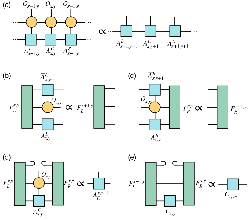
Figure 18: The key steps of the multi-site VUMPS algorithm. (b) and (c) Eigen-equations to update the left and right environmental fixed points of the channel operators. (e) and (f) Eigen-equations to update the central tensors based on the new environment.

The key process of the algorithm is summarized in Figs. 18 (b)-(e), including sequentially solving the left and right fixed points of the channel operators

$$\mathbb{T}_{L}^{(x,y)}F_{L}^{(x,y)} =\lambda_{(x,y)}F_{L}^{(x+1,y)},$$ (56)

$$\mathbb{T}_{R}^{(x,y)}F_{R}^{(x,y)} =\lambda_{(x,y)}F_{R}^{(x-1,y)},$$ (57)

and the updating of the central tensors

$$H_{A_{C}}^{(x,y)}A_{C}^{(x,y)} =\lambda A_{C}^{(x,y+1)},$$ (58)

$$H_{C}^{(x,y)}C^{(x,y)} =C^{(x,y+1)}.$$ (59)

Note that, when solving the fixed point eigen equation (A.8)-(A.11), one may not directly use the linear transfer matrix composed by the uniform local tensor ${O}$, but the interior structure should be explored. This will significantly reduce the computational complexity.

A.2 Physical quantities

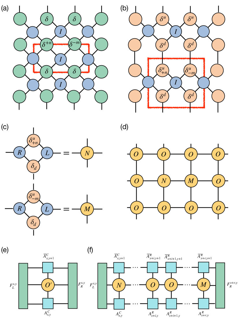
Figure 19: (a) The imbalanced delta tensors as a result of imbalanced currents introduced by the local observables. (b) The vertical split of the imbalanced delta tensors. (c) The construction of the impurity tensors from imbalanced delta tensors. (d) Two impurity tensors are introduced into the original tensor network. (e) Expectation of a local observable by contracting the leading eigenvectors of the channel operators. (f) Two-point correlation functions calculated by contracting a sequence of channel operators.

From the fixed-point MPS for the 1D quantum transfer operator, various physical quantities can be estimated accurately. The entanglement properties can be detected via the Schmidt decomposition of $|\Psi(A)\rangle^{(y)}$ which bipartites the relevant 1D quantum state of the MPO, and the entanglement entropy can be determined directly from the singular values $s_{\alpha}$ as

$$S_{E}=-\sum_{\alpha=1}^{D}s_{\alpha}^{2}\ln s_{\alpha}^{2},$$ (60)

in correspondence to the quantum entanglement measure.

Moreover, the expectation value of a local observable can be evaluated by inserting the corresponding impurity tensor into the original tensor network for the partition function. The impurity tensors can be obtained simply by introducing an unbalanced delta tensor to replace the original delta tensor characterizing the constraints of sharing spins.

For Ising spins, the expectation value of a local spin at site $j$ can be expressed as

$$\langle s_{j}\rangle=\frac{1}{Z}\sum_{\{s_{i}=\pm 1\}}\mathrm{e}^{-\beta E(\{s_{i}\})}s_{j}$$ (61)

where $E(\{s_{i}\})$ is the energy of a state under a given spin configuration $\{s_{i}\}$. The $s_{j}$ term just changes the Kronecker delta tensor from the form of (16) to

$$\delta_{s_{1},s_{2},\cdots,s_{n}}=\begin{cases}s_{1},&s_{1}=s_{2}=\cdots=s_{n}\\ 0,&\text{otherwise}\end{cases}.$$ (62)

For XY spins, the expectation value of $\mathrm{e}^{iq\theta}$ can be calculated by introducing imbalanced currents into the original delta tensors from the conservation form of (III.3) to

$$\delta^{q}=\delta_{n_{1}+n_{2}+n_{3}+n_{4}+q,0}$$ (63)

as displayed in Fig. 19 (a). Accordingly, the vertical splitting of the delta tensor in (39) should be be modified to

$$\delta_{n_{1}+n_{2}+n_{3}+n_{4}+q,0}=\sum_{n_{5}}\delta_{n_{1}+n_{2}-n_{5},0}^{u}\delta_{n_{1}+n_{2}+n_{5}+q,0}^{d}$$ (64)

as shown in Fig. 19 (b). Then the impurity tensors can be constructed in the same way by including the imbalanced delta tensors as depicted in Fig. 19 (c). The tensor network containing two impurity tensors is displayed in Fig. 19 (d) as an example.

Using the MPS fixed point, the contraction of the tensor network containing the impurity tensor is reduced to a trace of an infinite sequence of channel operators, which can be further squeezed into a contraction of a small network. As shown in Fig. 19 (e), the evaluation of a single variable is expressed as a contraction of only five tensors. And the expectation value of the two-point correlation function

$$G(r)=\langle\cos(n\theta_{i}-m\theta_{i+r})\rangle$$ (65)

can be reduced to a trace of a row of channel operators containing two impurity tensors as shown in Fig. 19 (f).

References

- Lacroix et al. (2011) C. Lacroix, P. Mendels, and F. Mila, Introduction to Frustrated Magnetism: Materials, Experiments, Theory, Springer Series in Solid-State Sciences (Springer Berlin Heidelberg, 2011), ISBN 9783642105890, URL https://books.google.com/books?id=utSV09ZuhOkC.
- Ramirez (1994) A. P. Ramirez, Annual Review of Materials Science 24, 453 (1994), eprint https://doi.org/10.1146/annurev.ms.24.080194.002321, URL https://doi.org/10.1146/annurev.ms.24.080194.002321.
- Moessner (2001) R. Moessner, Canadian Journal of Physics 79, 1283 (2001), eprint https://doi.org/10.1139/p01-123, URL https://doi.org/10.1139/p01-123.
- Diep (2020) H. T. Diep, Frustrated Spin Systems (WORLD SCIENTIFIC, 2020), 3rd ed., eprint https://www.worldscientific.com/doi/pdf/10.1142/11660, URL https://www.worldscientific.com/doi/abs/10.1142/11660.
- Ortiz-Ambriz et al. (2019) A. Ortiz-Ambriz, C. Nisoli, C. Reichhardt, C. J. O. Reichhardt, and P. Tierno, Rev. Mod. Phys. 91, 041003 (2019), URL https://link.aps.org/doi/10.1103/RevModPhys.91.041003.
- Sadoc and Mosseri (1999) J.-F. Sadoc and R. Mosseri, Introduction to geometrical frustration (Cambridge University Press, 1999), p. 1–13, Collection Alea-Saclay: Monographs and Texts in Statistical Physics.
- Wannier (1950) G. H. Wannier, Phys. Rev. 79, 357 (1950), URL https://link.aps.org/doi/10.1103/PhysRev.79.357.
- Kanô and Naya (1953) K. Kanô and S. Naya, Progress of Theoretical Physics 10, 158 (1953), ISSN 0033-068X, eprint https://academic.oup.com/ptp/article-pdf/10/2/158/5229090/10-2-158.pdf, URL https://doi.org/10.1143/ptp/10.2.158.
- Teitel and Jayaprakash (1983) S. Teitel and C. Jayaprakash, Phys. Rev. B 27, 598 (1983), URL https://link.aps.org/doi/10.1103/PhysRevB.27.598.
- Thijssen and Knops (1990) J. M. Thijssen and H. J. F. Knops, Phys. Rev. B 42, 2438 (1990), URL https://link.aps.org/doi/10.1103/PhysRevB.42.2438.
- Ramirez-Santiago and José (1992) G. Ramirez-Santiago and J. V. José, Phys. Rev. Lett. 68, 1224 (1992), URL https://link.aps.org/doi/10.1103/PhysRevLett.68.1224.
- Granato and Nightingale (1993) E. Granato and M. P. Nightingale, Phys. Rev. B 48, 7438 (1993), URL https://link.aps.org/doi/10.1103/PhysRevB.48.7438.
- Lee (1994) J.-R. Lee, Phys. Rev. B 49, 3317 (1994), URL https://link.aps.org/doi/10.1103/PhysRevB.49.3317.
- Lee and Lee (1994) S. Lee and K.-C. Lee, Phys. Rev. B 49, 15184 (1994), URL https://link.aps.org/doi/10.1103/PhysRevB.49.15184.
- Ramirez-Santiago and José (1994) G. Ramirez-Santiago and J. V. José, Phys. Rev. B 49, 9567 (1994), URL https://link.aps.org/doi/10.1103/PhysRevB.49.9567.
- Olsson (1995) P. Olsson, Phys. Rev. Lett. 75, 2758 (1995), URL https://link.aps.org/doi/10.1103/PhysRevLett.75.2758.
- Cataudella and Nicodemi (1996) V. Cataudella and M. Nicodemi, Physica A: Statistical Mechanics and its Applications 233, 293 (1996), ISSN 0378-4371, URL https://www.sciencedirect.com/science/article/pii/S0378437196002105.
- Olsson (1997) P. Olsson, Phys. Rev. B 55, 3585 (1997), URL https://link.aps.org/doi/10.1103/PhysRevB.55.3585.
- Boubcheur and Diep (1998) E. H. Boubcheur and H. T. Diep, Phys. Rev. B 58, 5163 (1998), URL https://link.aps.org/doi/10.1103/PhysRevB.58.5163.
- Hasenbusch et al. (2005) M. Hasenbusch, A. Pelissetto, and E. Vicari, J. Stat. Mech. 2005, P12002 (2005), URL https://doi.org/10.1088/1742-5468/2005/12/p12002.
- Okumura et al. (2011) S. Okumura, H. Yoshino, and H. Kawamura, Phys. Rev. B 83, 094429 (2011), URL https://link.aps.org/doi/10.1103/PhysRevB.83.094429.
- Nussinov (2014) Z. Nussinov, Journal of Statistical Mechanics: Theory and Experiment 2014, P02012 (2014), URL https://doi.org/10.1088/1742-5468/2014/02/p02012.
- Lima et al. (2019) A. B. Lima, L. A. S. Mól, and B. V. Costa, Journal of Statistical Physics 175, 960 (2019), URL https://doi.org/10.1007/s10955-019-02271-x.
- Song and Zhang (2022) F.-F. Song and G.-M. Zhang, Phys. Rev. B 105, 134516 (2022), URL https://link.aps.org/doi/10.1103/PhysRevB.105.134516.
- Miyashita and Shiba (1984) S. Miyashita and H. Shiba, Journal of the Physical Society of Japan 53, 1145 (1984), eprint https://doi.org/10.1143/JPSJ.53.1145, URL https://doi.org/10.1143/JPSJ.53.1145.
- Shih and Stroud (1984) W. Y. Shih and D. Stroud, Phys. Rev. B 30, 6774 (1984), URL https://link.aps.org/doi/10.1103/PhysRevB.30.6774.
- Lee et al. (1984) D. H. Lee, J. D. Joannopoulos, J. W. Negele, and D. P. Landau, Phys. Rev. Lett. 52, 433 (1984), URL https://link.aps.org/doi/10.1103/PhysRevLett.52.433.
- Lee et al. (1986) D. H. Lee, J. D. Joannopoulos, J. W. Negele, and D. P. Landau, Phys. Rev. B 33, 450 (1986), URL https://link.aps.org/doi/10.1103/PhysRevB.33.450.
- Korshunov and Uimin (1986) S. E. Korshunov and G. V. Uimin, Journal of Statistical Physics 43, 1 (1986), URL https://doi.org/10.1007/BF01010569.
- Van Himbergen (1986) J. E. Van Himbergen, Phys. Rev. B 33, 7857 (1986), URL https://link.aps.org/doi/10.1103/PhysRevB.33.7857.
- Xu and Southern (1996) H.-J. Xu and B. W. Southern, J. Phys. A: Math. Gen. 29, L133 (1996), URL https://doi.org/10.1088/0305-4470/29/5/009.
- Lee and Lee (1998) S. Lee and K.-C. Lee, Phys. Rev. B 57, 8472 (1998), URL https://link.aps.org/doi/10.1103/PhysRevB.57.8472.
- Capriotti et al. (1998) L. Capriotti, R. Vaia, A. Cuccoli, and V. Tognetti, Phys. Rev. B 58, 273 (1998), URL https://link.aps.org/doi/10.1103/PhysRevB.58.273.
- Harris et al. (1992) A. B. Harris, C. Kallin, and A. J. Berlinsky, Phys. Rev. B 45, 2899 (1992), URL https://link.aps.org/doi/10.1103/PhysRevB.45.2899.
- Rzchowski (1997) M. S. Rzchowski, Phys. Rev. B 55, 11745 (1997), URL https://link.aps.org/doi/10.1103/PhysRevB.55.11745.
- Cherepanov et al. (2001) V. B. Cherepanov, I. V. Kolokolov, and E. V. Podivilov, Journal of Experimental and Theoretical Physics Letters 74, 596 (2001), URL https://doi.org/10.1134/1.1455068.
- Park and Huse (2001) K. Park and D. A. Huse, Phys. Rev. B 64, 134522 (2001), URL https://link.aps.org/doi/10.1103/PhysRevB.64.134522.
- Korshunov (2002) S. E. Korshunov, Phys. Rev. B 65, 054416 (2002), URL https://link.aps.org/doi/10.1103/PhysRevB.65.054416.
- Andreanov and Fistul (2020) A. Andreanov and M. V. Fistul, Phys. Rev. B 102, 140405 (2020), URL https://link.aps.org/doi/10.1103/PhysRevB.102.140405.
- Song and Zhang (2023) F.-F. Song and G.-M. Zhang, Phys. Rev. B 108, 014424 (2023), URL https://link.aps.org/doi/10.1103/PhysRevB.108.014424.
- Villain (1977a) J. Villain, Journal of Physics C: Solid State Physics 10, 1717 (1977a), URL https://doi.org/10.1088/0022-3719/10/10/014.
- Binder and Young (1986) K. Binder and A. P. Young, Rev. Mod. Phys. 58, 801 (1986), URL https://link.aps.org/doi/10.1103/RevModPhys.58.801.
- Hartmann and Rieger (2001) A. H. Hartmann and H. Rieger, Approximation Methods for Spin Glasses (John Wiley & Sons, Ltd, 2001), chap. 9, pp. 185–226, ISBN 9783527600878, eprint https://onlinelibrary.wiley.com/doi/pdf/10.1002/3527600876.ch9, URL https://onlinelibrary.wiley.com/doi/abs/10.1002/3527600876.ch9.
- Swendsen and Wang (1987) R. H. Swendsen and J.-S. Wang, Phys. Rev. Lett. 58, 86 (1987), URL https://link.aps.org/doi/10.1103/PhysRevLett.58.86.
- Wolff (1989) U. Wolff, Phys. Rev. Lett. 62, 361 (1989), URL https://link.aps.org/doi/10.1103/PhysRevLett.62.361.
- Rakala and Damle (2017) G. Rakala and K. Damle, Phys. Rev. E 96, 023304 (2017), URL https://link.aps.org/doi/10.1103/PhysRevE.96.023304.
- Vanderstraeten et al. (2018) L. Vanderstraeten, B. Vanhecke, and F. Verstraete, Phys. Rev. E 98, 042145 (2018), URL https://link.aps.org/doi/10.1103/PhysRevE.98.042145.
- Vanhecke et al. (2021) B. Vanhecke, J. Colbois, L. Vanderstraeten, F. Verstraete, and F. Mila, Phys. Rev. Research 3, 013041 (2021), URL https://link.aps.org/doi/10.1103/PhysRevResearch.3.013041.
- Colbois et al. (2022) J. Colbois, B. Vanhecke, L. Vanderstraeten, A. Smerald, F. Verstraete, and F. Mila, Phys. Rev. B 106, 174403 (2022), URL https://link.aps.org/doi/10.1103/PhysRevB.106.174403.
- Blote and Hilborst (1982) H. W. J. Blote and H. J. Hilborst, Journal of Physics A: Mathematical and General 15, L631 (1982), URL https://dx.doi.org/10.1088/0305-4470/15/11/011.
- Chalker (2017) J. T. Chalker, in Topological Aspects of Condensed Matter Physics: Lecture Notes of the Les Houches Summer School: Volume 103, August 2014 (Oxford University Press, 2017), ISBN 9780198785781, eprint https://academic.oup.com/book/0/chapter/203968137/chapter-pdf/45121870/acprof-9780198785781-chapter-3.pdf, URL https://doi.org/10.1093/acprof:oso/9780198785781.003.0003.
- Zauner-Stauber et al. (2018) V. Zauner-Stauber, L. Vanderstraeten, M. T. Fishman, F. Verstraete, and J. Haegeman, Phys. Rev. B 97, 045145 (2018), URL https://link.aps.org/doi/10.1103/PhysRevB.97.045145.
- Vanderstraeten et al. (2019a) L. Vanderstraeten, J. Haegeman, and F. Verstraete, SciPost Phys. Lect. Notes p. 7 (2019a), URL https://scipost.org/10.21468/SciPostPhysLectNotes.7.
- Nietner et al. (2020) A. Nietner, B. Vanhecke, F. Verstraete, J. Eisert, and L. Vanderstraeten, Quantum 4, 328 (2020), ISSN 2521-327X, URL https://doi.org/10.22331/q-2020-09-21-328.
- Haegeman and Verstraete (2017) J. Haegeman and F. Verstraete, Annual Review of Condensed Matter Physics 8, 355 (2017), eprint https://doi.org/10.1146/annurev-conmatphys-031016-025507, URL https://doi.org/10.1146/annurev-conmatphys-031016-025507.
- Zhao et al. (2010) H. H. Zhao, Z. Y. Xie, Q. N. Chen, Z. C. Wei, J. W. Cai, and T. Xiang, Phys. Rev. B 81, 174411 (2010), URL https://link.aps.org/doi/10.1103/PhysRevB.81.174411.
- Levin and Nave (2007) M. Levin and C. P. Nave, Phys. Rev. Lett. 99, 120601 (2007), URL https://link.aps.org/doi/10.1103/PhysRevLett.99.120601.
- Yu et al. (2014) J. F. Yu, Z. Y. Xie, Y. Meurice, Y. Liu, A. Denbleyker, H. Zou, M. P. Qin, J. Chen, and T. Xiang, Phys. Rev. E 89, 013308 (2014), URL https://link.aps.org/doi/10.1103/PhysRevE.89.013308.
- Vanderstraeten et al. (2019b) L. Vanderstraeten, B. Vanhecke, A. M. Läuchli, and F. Verstraete, Phys. Rev. E 100, 062136 (2019b), URL https://link.aps.org/doi/10.1103/PhysRevE.100.062136.
- Fishman et al. (2018) M. T. Fishman, L. Vanderstraeten, V. Zauner-Stauber, J. Haegeman, and F. Verstraete, Phys. Rev. B 98, 235148 (2018), URL https://link.aps.org/doi/10.1103/PhysRevB.98.235148.
- Kosterlitz and Thouless (1973) J. M. Kosterlitz and D. J. Thouless, Journal of Physics C: Solid State Physics 6, 1181 (1973), URL https://dx.doi.org/10.1088/0022-3719/6/7/010.
- Kosterlitz (1974) J. M. Kosterlitz, Journal of Physics C: Solid State Physics 7, 1046 (1974), URL https://dx.doi.org/10.1088/0022-3719/7/6/005.
- Minnhagen (1987) P. Minnhagen, Reviews of Modern Physics 59, 1001 (1987).
- Vallat and Beck (1994) A. Vallat and H. Beck, Physical Review B 50, 4015 (1994).
- Villain (1977b) J. Villain, Journal of Physics C: Solid State Physics 10, 4793 (1977b), URL https://doi.org/10.1088/0022-3719/10/23/013.
- Obuchi and Kawamura (2012) T. Obuchi and H. Kawamura, Journal of the Physical Society of Japan 81, 054003 (2012), eprint https://doi.org/10.1143/JPSJ.81.054003, URL https://doi.org/10.1143/JPSJ.81.054003.
- Lv et al. (2013) J.-P. Lv, T. M. Garoni, and Y. Deng, Phys. Rev. B 87, 024108 (2013), URL https://link.aps.org/doi/10.1103/PhysRevB.87.024108.
- Maccari et al. (2020) I. Maccari, N. Defenu, L. Benfatto, C. Castellani, and T. Enss, Physical Review B 102, 104505 (2020), URL https://link.aps.org/doi/10.1103/PhysRevB.102.104505.
- Maccari et al. (2023) I. Maccari, N. Defenu, C. Castellani, and T. Enss, Journal of Physics: Condensed Matter 35, 334001 (2023), URL https://dx.doi.org/10.1088/1361-648X/acd295.
- Minnhagen (1985a) P. Minnhagen, Physical Review B 32, 3088 (1985a).
- Minnhagen (1985b) P. Minnhagen, Physical Review Letters 54, 2351 (1985b).
- Zhang et al. (1993) G.-M. Zhang, H. Chen, and X. Wu, Phys. Rev. B 48, 12304 (1993), URL https://link.aps.org/doi/10.1103/PhysRevB.48.12304.
- Swendsen (1982) R. H. Swendsen, Physical Review Letters 49, 1302 (1982).
- Lee and Teitel (1990) J.-R. Lee and S. Teitel, Physical Review Letters 64, 1483 (1990).
- Lee and Teitel (1991) J.-R. Lee and S. Teitel, Physical Review Letters 66, 2100 (1991).
- Lidmar and Wallin (1997) J. Lidmar and M. Wallin, Physical Review B 55, 522 (1997).
- Kohring et al. (1986) G. Kohring, R. E. Shrock, and P. Wills, Physical Review Letters 57, 1358 (1986).
- Shenoy (1990) S. R. Shenoy, Physical Review B 42, 8595 (1990).
- Kamlapure et al. (2010) A. Kamlapure, M. Mondal, M. Chand, A. Mishra, J. Jesudasan, V. Bagwe, L. Benfatto, V. Tripathi, and P. Raychaudhuri, Applied Physics Letters 96, 072509 (2010).
- Mondal et al. (2011) M. Mondal, S. Kumar, M. Chand, A. Kamlapure, G. Saraswat, G. Seibold, L. Benfatto, and P. Raychaudhuri, Physical Review Letters 107, 217003 (2011).
- Chen et al. (1992) M. T. Chen, J. M. Roesler, and J. M. Mochel, Journal of Low Temperature Physics 89, 125 (1992), URL https://doi.org/10.1007/BF00692584.
- Zhang (1993) S.-C. Zhang, Physical Review Letters 71, 2142 (1993), URL https://link.aps.org/doi/10.1103/PhysRevLett.71.2142.
- Gabay and Kapitulnik (1993) M. Gabay and A. Kapitulnik, Physical Review Letters 71, 2138 (1993), URL https://link.aps.org/doi/10.1103/PhysRevLett.71.2138.
- Botelho and Sá de Melo (2006) S. S. Botelho and C. A. R. Sá de Melo, Physical Review Letters 96, 040404 (2006).
- Hivet et al. (2014) R. Hivet, E. Cancellieri, T. Boulier, D. Ballarini, D. Sanvitto, F. M. Marchetti, M. H. Szymanska, C. Ciuti, E. Giacobino, and A. Bramati, Phys. Rev. B 89, 134501 (2014), URL https://link.aps.org/doi/10.1103/PhysRevB.89.134501.
- Granato and Kosterlitz (1986) E. Granato and J. M. Kosterlitz, Physical Review B 33, 4767 (1986).
- Granato (1987) E. Granato, Journal of Physics C: Solid State Physics 20, L215 (1987).
- Lee et al. (1991) J. Lee, E. Granato, and J. M. Kosterlitz, Physical Review B 44, 4819 (1991).
- Li and Cieplak (1994) M. S. Li and M. Cieplak, Physical Review B 50, 955 (1994).
- Nightingale et al. (1995) M. P. Nightingale, E. Granato, and J. M. Kosterlitz, Physical Review B 52, 7402 (1995).
- Halperin and Nelson (1978) B. I. Halperin and D. R. Nelson, Phys. Rev. Lett. 41, 121 (1978), URL https://link.aps.org/doi/10.1103/PhysRevLett.41.121.
- Nelson and Halperin (1979) D. R. Nelson and B. I. Halperin, Phys. Rev. B 19, 2457 (1979), URL https://link.aps.org/doi/10.1103/PhysRevB.19.2457.
- Young (1979) A. P. Young, Phys. Rev. B 19, 1855 (1979), URL https://link.aps.org/doi/10.1103/PhysRevB.19.1855.
- Mizoguchi et al. (2017) T. Mizoguchi, L. D. C. Jaubert, and M. Udagawa, Phys. Rev. Lett. 119, 077207 (2017), URL https://link.aps.org/doi/10.1103/PhysRevLett.119.077207.
- Tokushuku et al. (2019) K. Tokushuku, T. Mizoguchi, and M. Udagawa, Phys. Rev. B 100, 134415 (2019), URL https://link.aps.org/doi/10.1103/PhysRevB.100.134415.
- Tokushuku et al. (2020) K. Tokushuku, T. Mizoguchi, and M. Udagawa, Journal of the Physical Society of Japan 89, 053708 (2020), eprint https://doi.org/10.7566/JPSJ.89.053708, URL https://doi.org/10.7566/JPSJ.89.053708.
- Chalker et al. (1992) J. T. Chalker, P. C. W. Holdsworth, and E. F. Shender, Phys. Rev. Lett. 68, 855 (1992), URL https://link.aps.org/doi/10.1103/PhysRevLett.68.855.
- Pitts et al. (2022) J. Pitts, F. L. Buessen, R. Moessner, S. Trebst, and K. Shtengel, Phys. Rev. Res. 4, 043019 (2022), URL https://link.aps.org/doi/10.1103/PhysRevResearch.4.043019.